periodic delta function and expansion in legendre polynomials

Gauge Institute Journal H. Vic Dannon

Periodic Delta Function, and Expansion in Legendre

Polynomials H. Vic Dannon

[email protected] June, 2012

Abstract Let ( )f x be defined on [ 1 , so that ,1]− (1) ( 1)f f= − ,

and let be the Legendre Polynomials on [ 1 , ( )nP x ,1]−

0( ) 1P x = , , 1( )P x x= 23 12 2 2( )P x x= − , 35

3 2( )P x x x= − 3

2,…

The Legendre Series associated with ( )f x is

0 0 1 1 2 2( ) ( ) ( ) ....a P x a P x a P x+ + + where

12 1

21

( ) ( )nn na f P

ξ

ξ

ξ ξ=

+

=−

= ∫ dξ

are the Legendre coefficients.

The Legendre Series Theorem supplies the conditions under which

the Legendre Series associated with ( )f x equals ( )f x .

It is believed to hold in the Calculus of Limits for smooth enough

function. In fact,

1


The Theorem cannot be proved in the Calculus of Limits

under any conditions,

because the summation of the Legendre Series requires

integration over the periodically singular Legendre Kernel.

Plots of partial sums of the Legendre Series speak volumes about

the sensibility of the claims to have infinities bound by epsilons.

In Infinitesimal Calculus, the Legendre Kernel

1 3 50 0 1 1 2 22 2 2(cos ) (cos ) (cos ) (cos ) (cos ) (cos ) ...x xP P P P P Pξ ξ ξθ θ θ θ θ θ+ + x +

..

)θ

is the Periodic Delta Function,

( ) ... ( 2 ) ( ) ( 2 ) .Periodic x x x xξ ξ ξ ξδ θ θ δ θ θ π δ θ θ δ θ θ π− = + − + + − + − − + .

(Periodic xξδ θ − equals its Legendre Series, and the Legendre Series

associated with any periodic hyper-real integrable ( )f x , equals

( )f x .

Keywords: Infinitesimal, Infinite-Hyper-Real, Hyper-Real,

infinite Hyper-real, Infinitesimal Calculus, Delta Function,

Legendre Polynomials, Legendre Coefficients, Periodic Delta

Function, Delta Comb, Legendre Series, Legendre Kernel,

Expansion in Legendre Polynomials,

2000 Mathematics Subject Classification 26E35; 26E30;

26E15; 26E20; 26A06; 26A12; 03E10; 03E55; 03E17; 03H15;

46S20; 97I40; 97I30.

2


Contents

0. The Origin of the Legendre Series Theorem

1. Divergence of the Legendre Kernel in the Calculus of Limits

2. Hyper-real line.

3. Integral of a Hyper-real Function

4. Delta Function

5. Periodic Delta Function, ( )Periodic xξδ θ − θ

θ

θ

θ

6. Convergent Series

7. Legendre Sequence and ( )Periodic xξδ θ −

8. Legendre Kernel and . ( )Periodic xξδ θ −

9. Legendre Series of ( )Periodic xξδ θ −

10. Legendre Series Theorem

References

3


The Origin of the Legendre Series

Theorem The Legendre Polynomials on [ 1 ,1]−

0( ) 1P x = , , 1( )P x x= 23 12 2 2( )P x x= − , 35

3 2( )P x x x= − 3

2,…,

are the orthogonal functions generated in the Gram-Schmidt

orthogonalization so that.

1

22 1

1

( ) ( )x

m n mnx

P x P x dx δ=

+=−

=∫ n .

0.1 Legendre

generated the polynomials by expanding

12

2

1[1 (2 )]

1 2x

xα α

α α

−= − −− +

by the Binomial Theorem.

In the Binomial Expansion,

2 2 3 31 1 3 1 3 52 2 4 2 4 6

1 (2 ) (2 ) (2 )x x xα α α α α α⋅ ⋅ ⋅⋅ ⋅ ⋅

+ − + − + − + ...,

the coefficient of is 0α

0( ) 1P x = ,

the coefficient of is 1α

1( )P x x= ,

the coefficient of is 2α23 1

2 2 2( )P x x= − ,

4


the coefficient of is 3α31

3 2( ) (5 3 )P x x x= − ,

…………………………

0.2 Legendre Differential Equation

Laplace Equation in radial coordinates for a potential is ( , , )V r θ φ

22 21 1

sin sin( ) (sin )r rr V V Vθ θ φθ θ

θ∂ ∂ + ∂ ∂ + ∂ = 0 .

Assuming that

( , , ) ( ) ( ) ( )V r R rθ φ θ φ= Θ Φ ,

the Laplace equation becomes

221 1 1

sin sin( ')' (sin ')' ''Rr R

θ θθ

Θ Φ+ Θ + Φ 0= .

Then, 21

1( ')'Rr R const C= ≡ .

Substituting a linear combination of

nr , and 1

1nr +

the equation for R yields

1( 1)n n C+ =

and the Laplace Equation becomes

2 sin 1( 1)sin (sin ')' '' 0n n θθ θΘ Φ

+ + Θ + Φ = .

Then, 1

2'' const CΦΦ = ≡ .

To obtain solutions , and , we set ime φ ime φ−

5


2C m≡ − ,

and the Laplace Equation becomes an equation for , ( )θΘ

2

21

sin sin( 1) ( ' sin )' mn n

θ θθ+ Θ+ Θ − Θ = 0 .

Denoting cosx θ≡ ,

( ) ( )X x θ= Θ ,

' 'd dX dx

Xd dx d

θθ θΘ

Θ = = = − sin ,

2

2'' { ' sin }d d

Xdd

θθθ

ΘΘ = = − ,

'sin ' cos

dX dxX

dx dθ θ

θ= − − ,

, 2'' sin ' cosX Xθ θ= −

1 csin sin

( ' sin )' '' ' θθ θ

θΘ = Θ + Θ os ,

2 cossin

'' sin ' cos ' sinX X X θθ

θ θ θ= − − ,

, 2(1 ) '' 2 'x X xX= − −

, 2[(1 ) ']'x X= −

the Laplace Equation becomes

2

22

1[(1 ) ']' [ ( 1) ] 0m

xx X n n X

−− + + − = .

For , it is the Legendre equation 0m =

2(1 ) '' 2 ' ( 1) 0x X xX n n X− − + + = .

6


Substituting in it

2 10 1 2 1 2( ) ... ...l l l

l l lX x c c x c x c x c x c x+ ++ += + + + + + + +2

0l =

0l

,

we have

2 2 1

2 2 1

2 2 2

0 0 0 0

( 1) ( 1)

2 ( 1)

l l ll l l

l l ll l l

l l l ll l l

x l x l x l ll l l l

l lc x l lc x lc x

D c x x D c x x D c x n n c x

=∞ =∞ =∞− − −

= = =

=∞ =∞ =∞ =∞

= = = =

− −

− − + +

∑ ∑ ∑

∑ ∑ ∑ ∑ ,

20

{( 1)( 2) ( 1) 2 ( 1) } 0l

ll l l l

l

l l c l l c lc n n c x=∞

+=

+ + − − − + + =∑ ,

2( 1)( 2) ( 1) 2 ( 1)l l ll l c l l c lc n n c++ + − − − + + = ,

2( 1) 2 ( 1)

( 1)( 2)l ll l l n n

c cl l+

− + − +=

+ +

2( )( 1)

( 1)( 1)( 2)l ln l n l

c cl l+− + −

= −+ +

The solution is

( 1) ( 1)( 2)2 30 1 0 11 2 1 2 3

( ) n n n nX x c c x c x c x+ − +⋅ ⋅ ⋅

= + − − +

( 1)( 2)( 3) ( 1)( 2)( 3)( 4)4 50 11 2 3 4 1 2 3 4 5

...n n n n n n n nc x c+ − + − + − +⋅ ⋅ ⋅ ⋅ ⋅ ⋅ ⋅

+ + x +

( 1) ( 1)( 2)( 3)2 40 1 2 1 2 3 4{1 ...}n n n n n nc x x+ + − +

⋅ ⋅ ⋅ ⋅= − + − +

( 1)( 2) ( 1)( 2)( 3)( 4)2 41 1 2 3 1 2 3 4 5

{1 ...}n n n n n nc x x x− + − + − +⋅ ⋅ ⋅ ⋅ ⋅ ⋅

+ − + + .

Therefore, for , the series terms vanish for 2n = k 0c

2 2,2 4,...k k+ + ,

7


and we obtain the Legendre Polynomials. 2 ( )kP x

for , the series terms vanish for 2n k= + 1 1c

2 3,2 5,...k k+ +

and we obtain the Legendre Polynomials. 2 1( )kP x+

A solution for is the infinite linear combination ( )θΘ

0 0 1 1 2 2( ) ( ) ( ) ....P x P x P xα α α+ + +

0.3 The Legendre Series Associated with a periodic ( )f x

Let ( )f x be integrable on [ 1 , so that ,1]− (1) ( 1)f f= − , and let

be the Legendre Polynomials on [ 1 , ( )nP x

,1]−

0( ) 1P x = , , 1( )P x x= 23 12 2 2( )P x x= − , 35

3 2( )P x x x= − 3

2,…

The Polynomials are orthogonal on [ 1 . That is, ,1]−

1

22 1

1

( ) ( )x

m n mnx

P x P x dx δ=

+=−

=∫ n

If ( )f x can be expanded in the Legendre Polynomials,

0 0 1 1 2 2( ) ( ) ( ) ( ) ....f x a P x a P x a P x= + + + ,

Then,

1 1

0 0 1 1 2 21 1

( ) ( ) { ( ) ( ) ( ) ....} ( )x x

n nx x

f x P x dx a P x a P x a P x P x dx= =

=− =−

= + + +∫ ∫

8


2 2 20 1 22 1 2 1 2 1

1 1 1

0 0 1 1 2 21 1 1

( ) ( ) ( ) ( ) ( ) ( ) ...

n n nn n n

x x x

n nx x x

a P x P x a P x P x a P x P x

δ δ δ+ + +

= = =

=− =− =−

= + +∫ ∫ ∫ n +

22 1n n

a+

= .

Thus, the Legendre coefficients are

12 1

21

( ) ( )nn na f P

ξ

ξ

ξ ξ=

+

=−

= ∫ dξ .


0 0 1 1 2 2( ) ( ) ( ) ....a P x a P x a P x+ + + .

Since cosx θ= ,

the Legendre Polynomials,

( ) (cos )n nP x P θ= ,

are periodic in θ , with period 2 . π

Thus, the Legendre Polynomials are defined for any real

, arccos( ) 2x mθ π= +

where , and m is an integer. 1 1x− ≤ ≤

Therefore, the Legendre Series is periodic in , with period 2 . θ π

The Legendre Series Theorem supplies the conditions under which

the Legendre Series associated with ( )f x equals ( )f x .

Then, the function must be periodic too.

9


1.

Divergence of the Legendre

Kernel in the Calculus of Limits

for the Legendre Series to equal its function reflect the belief that

a smooth enough function equals its Legendre Series.

In fact, in the Calculus of Limits, no smoothness of the function

guarantees even the convergence of the Legendre Series.

1.1 The Legendre Kernel is either singular or zero

In the Calculus of Limits, the Legendre Series is the limit of the

sequence of Partial Sums

{ } 0 0 1 1( ) ( ) ( ) ... ( )egendre n n nf x a P x a P x a P= + + +L S x

1 1 12 11 3

0 0 1 12 2 21 1 1

( ) ( ) ( ) ( ) ( ) ( ) ... ( ) ( ) ( )nn nf P d P x f P d P x f P d P x

ξ ξ ξ

ξ ξ ξ

ξ ξ ξ ξ ξ ξ ξ ξ ξ= = =

+

=− =− =−

⎛ ⎞ ⎛ ⎞ ⎛⎟ ⎟⎜ ⎜ ⎜⎟ ⎟⎜ ⎜ ⎜⎟ ⎟= + + +⎜ ⎜ ⎜⎟ ⎟⎜ ⎜ ⎜⎟ ⎟⎜ ⎜ ⎜⎟ ⎟⎝ ⎠ ⎝ ⎠ ⎝∫ ∫ ∫

⎞⎟⎟⎟⎟⎟⎟⎠

{ }1

2 11 30 0 1 12 2 2

1

( ) ( ) ( ) ( ) ( ) ... ( ) ( )nn nf P P x P P x P P x d

ξ

ξ

ξ ξ ξ ξ=

+

=−

= + + +∫ ξ .

As n , the Legendre Sequence → ∞

2 11 30 0 1 12 2 2( ) ( ) ( ) ( ) ... ( ) ( )n

n nP P x P P x P P xξ ξ ξ++ + +

becomes the Legendre Kernel,

10


2 11 30 0 1 12 2 2( ) ( ) ( ) ( ) ... ( ) ( ) ...n

n nP P x P P x P P xξ ξ ξ++ + + + ,

To see that it diverges for , we apply the Christoffel-Darboux

Summation Formula, [Abramowitz, p.335, #8.9.1], or [Gradshteyn,

p.986, #8.9.15]. And [Szego, p.43].

xξ =

1 10 0

( ) ( ) ( ) ( )( ) ( ) ... (2 1) ( ) ( ) ( 1) n n n n

n n

P P x P PP P x n P P x n

x

ξ ξξ ξ

ξ+ +−

+ + + = +−

x

x

.

For , xξ →

2 20 0 0( ) ( ) ... (2 1) ( ) ( ) ( ) ... (2 1) ( )n n nP P x n P P x P x n Pξ ξ+ + + → + + + ,

and

1 1( ) ( ) ( ) ( ) 0( 1) ( 1)

0n n n nP P x P P x

n nx

ξ ξξ

+ +−+ →

−+ .

Applying Bernoulli’s rule to the indeterminate limit,

1 11 1 ( ) ( ) ( ) ( )( ) ( ) ( ) ( )lim lim

( )n n n nn n n n

x x

D P P x D P P xP P x P P x

x Dξ ξ

ξ ξ ξ

ξ ξξ ξ

ξ ξ+ ++ +

→ →

−−=

− − x

x

1n

=

1 1lim[ '( ) ( ) '( ) ( )]n n n nxP P x P P

ξξ ξ+ +→

= −

1 1'( ) ( ) '( ) ( )n n n nP x P x P x P x+ += −

Therefore,

2 20 1( ) ... (2 1) ( ) ( 1)[ '( ) ( ) '( ) ( )]n n n nP x n P x n P x P x P x P x+ ++ + + = + − .

Since both , and solve the Legendre differential ( )nP x 1( )nP x+

equation, [Spiegel, p.146], 2

( )( )

(1 ) ''( ) 2 '( ) ( 1) ( ) 0b xa x

x y x x y x n n y x− − + + ,

11


we have, ( )( )

1 1'( ) ( ) '( ) ( ) ( )b xa xdx

n n n nP x P x P x P x const e−

+ +∫− =

2

21( )x

xdx

const e −∫=

2log(1 )( ) xconst e− −=

21

constconst

x= ≥

−,

for any . 1 1x− < <

Hence,

2 12 21 102 2 2( ) ... ( ) ( 1)n

nP x P x n const++ + ≥ + × .

and the Legendre Kernel diverges to at any . ∞ xξ =

Therefore, while the partial sums of the Legendre Series exist,

their limit does not. That is, due to the singularity at , the

Legendre Series does not converge in the Calculus of Limits.

xξ =

Avoiding the singularity at , by using the Cauchy Principal

Value of the integral does not recover the Theorem, because at any

, the Legendre Kernel vanishes, and the integral will be

identically zero, for any function

xξ =

xξ ≠

( )f x .

To see that the kernel vanishes for any , we apply the

Christoffel-Darboux Summation Formula, with .

xξ ≠

xξ ≠

1 10 0

( ) ( ) ( ) ( )( ) ( ) ... (2 1) ( ) ( ) ( 1) n n n n

n n


x

ξ ξξ ξ

ξ+ +−

+ + + = +−

x.

By Rodrigue’s Formula [Spiegel, p. 146],

12


212 !

( ) ( 1)n

n nn xnP x D x= − .

2 11 2 1 2 2 1 2 11

2 !( 1)!

1{ ( 1) ( 1) ( 1) ( 1) }

nn n n n n n n

x xn n

nD D x D D x

x ξ ξξ ξξ +

+ + ++

+= − − − −

−n+−

2 11 2 1 2 2 1 2 11

2 ! !

0, 0,

1{ ( 1) ( 1) ( 1) ( 1)nn n n n n n n

x xn n

nn

D D x D D xx ξ ξξ ξ

ξ ++ + +

→ →∞→ →∞

= − − − −−

}n+−

. 0, as n→ → ∞

That is, the Legendre Kernel vanishes for any . xξ ≠

Plots of the Legendre sequence confirm that

In the Calculus of Limits,

the Legendre kernel is either singular or zero

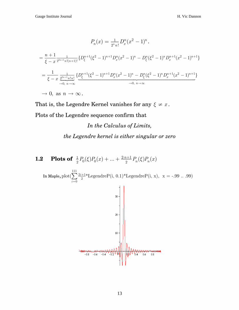
1.2 Plots of 2 110 02 2( ) ( ) ... ( ) ( )n

n nP P x P P xξ ξ⋅ ++ +

In Maple,111

2 12

0

plot( *LegendreP(i, 0.1)*LegendreP(i, x), x = -.99 .. .99)i

i

+

=∑

13


The pulse narrows with more terms:

In Maple, 365

2 12

0

plot( *LegendreP(i, 0.22)*LegendreP(i, x), x = -.9 .. .9)i

i

+

=∑

For , the pulses are periodic arccos( )xθ =

In Maple, 223

2 12

0

plot( *LegendreP(i, cos(2))*LegendreP(i, cos( )), = -7 .. 7)i

i

θ θ+

=∑

14


In Maple, 223

2 12

0

plot( *LegendreP(i, cos(0))*LegendreP(i, cos(x)), x = -13 .. 13)i

i

+

=∑

Thus, the Legendre Series Theorem cannot be proved in the

Calculus of Limits.

1.3 Infinitesimal Calculus Solution

By resolving the problem of the infinitesimals [Dan2], we obtained

the Infinite Hyper-reals that are strictly smaller than ∞ , and

constitute the value of the Delta Function at the singularity.

The controversy surrounding the Leibnitz Infinitesimals derailed

the development of the Infinitesimal Calculus, and the Delta

Function could not be defined and investigated properly.

In Infinitesimal Calculus, [Dan3], we can differentiate over jump

15


discontinuities, and integrate over singularities.

The Delta Function, the idealization of an impulse in Radar

circuits, is a Discontinuous Hyper-Real function which definition

requires Infinite Hyper-reals, and which analysis requires

Infinitesimal Calculus.

In [Dan5], we show that in infinitesimal Calculus, the hyper-real

1( )

2i xx e

ωω

ω

δ ωπ

=∞

=−∞

= ∫ d

is zero for any , 0x ≠

it spikes at , so that its Infinitesimal Calculus

integral is ,

0x =

( ) 1x

x

x dxδ=∞

=−∞

=∫

and 1(0)

dxδ = < ∞

}

.

Here, we show that in Infinitesimal calculus, the Legendre Kernel

is a periodic hyper-real Delta Function: A periodic train of Delta

Functions.

And the Legendre Series { ( )egendre f xL S associated with a Hyper-

real periodic function ( )f x , equals ( )f x .

16


2.

Hyper-real Line Each real number α can be represented by a Cauchy sequence of

rational numbers, so that . 1 2 3( , , ,...)r r r nr α→

The constant sequence ( is a constant hyper-real. , , ,...)α α α

In [Dan2] we established that,

1. Any totally ordered set of positive, monotonically decreasing

to zero sequences constitutes a family of

infinitesimal hyper-reals.

1 2 3( , , ,...)ι ι ι

2. The infinitesimals are smaller than any real number, yet

strictly greater than zero.

3. Their reciprocals (1 2 3

1 1 1, , ,...ι ι ι ) are the infinite hyper-reals.

4. The infinite hyper-reals are greater than any real number,

yet strictly smaller than infinity.

5. The infinite hyper-reals with negative signs are smaller

than any real number, yet strictly greater than −∞ .

6. The sum of a real number with an infinitesimal is a

non-constant hyper-real.

7. The Hyper-reals are the totality of constant hyper-reals, a

family of infinitesimals, a family of infinitesimals with

17


negative sign, a family of infinite hyper-reals, a family of

infinite hyper-reals with negative sign, and non-constant

hyper-reals.

8. The hyper-reals are totally ordered, and aligned along a

line: the Hyper-real Line.

9. That line includes the real numbers separated by the non-

constant hyper-reals. Each real number is the center of an

interval of hyper-reals, that includes no other real number.

10. In particular, zero is separated from any positive real

by the infinitesimals, and from any negative real by the

infinitesimals with negative signs, . dx−

11. Zero is not an infinitesimal, because zero is not strictly

greater than zero.

12. We do not add infinity to the hyper-real line.

13. The infinitesimals, the infinitesimals with negative

signs, the infinite hyper-reals, and the infinite hyper-reals

with negative signs are semi-groups with

respect to addition. Neither set includes zero.

14. The hyper-real line is embedded in , and is not

homeomorphic to the real line. There is no bi-continuous

one-one mapping from the hyper-real onto the real line.

∞

18


15. In particular, there are no points on the real line that

can be assigned uniquely to the infinitesimal hyper-reals, or

to the infinite hyper-reals, or to the non-constant hyper-

reals.

16. No neighbourhood of a hyper-real is homeomorphic to

an ball. Therefore, the hyper-real line is not a manifold. n

17. The hyper-real line is totally ordered like a line, but it

is not spanned by one element, and it is not one-dimensional.

19


3.

Integral of a Hyper-real Function

In [Dan3], we defined the integral of a Hyper-real Function.

Let ( )f x be a hyper-real function on the interval [ , . ]a b

The interval may not be bounded.

( )f x may take infinite hyper-real values, and need not be

bounded.

At each

a x≤ ≤ b ,

there is a rectangle with base 2

[ ,dx dxx x− +2], height ( )f x , and area

( )f x dx .

We form the Integration Sum of all the areas for the x ’s that

start at x , and end at x b , a= =

[ , ]

( )x a b

f x dx∈∑ .

If for any infinitesimal dx , the Integration Sum has the same

hyper-real value, then ( )f x is integrable over the interval [ , . ]a b

Then, we call the Integration Sum the integral of ( )f x from ,

to x , and denote it by

x a=

b=

20


( )x b

x a

f x dx=

=∫ .

If the hyper-real is infinite, then it is the integral over [ , , ]a b

If the hyper-real is finite,

( ) real part of the hyper-realx b

x a

f x dx=

=

=∫ .

3.1 The countability of the Integration Sum

In [Dan1], we established the equality of all positive infinities:

We proved that the number of the Natural Numbers,

Card , equals the number of Real Numbers, , and

we have

2CardCard =

2 2( ) .... 2 2 ...CardCardCard Card= = = = = ≡ ∞ .

In particular, we demonstrated that the real numbers may be

well-ordered.

Consequently, there are countably many real numbers in the

interval [ , , and the Integration Sum has countably many terms. ]a b

While we do not sequence the real numbers in the interval, the

summation takes place over countably many ( )f x dx .

The Lower Integral is the Integration Sum where ( )f x is replaced

21


by its lowest value on each interval 2 2

[ ,dx dxx x− + ]

3.2 2 2[ , ]

inf ( )dx dxx t xx a b

f t dx− ≤ ≤ +∈

⎛ ⎞⎟⎜ ⎟⎜ ⎟⎜ ⎟⎜⎝ ⎠∑

The Upper Integral is the Integration Sum where ( )f x is replaced

by its largest value on each interval 2 2

[ ,dx dxx x− + ]

3.3 2 2[ , ]

sup ( )dx dxx t xx a b

f t dx− ≤ ≤ +∈

⎛ ⎞⎟⎜ ⎟⎜ ⎟⎜ ⎟⎜ ⎟⎝ ⎠∑

If the integral is a finite hyper-real, we have

3.4 A hyper-real function has a finite integral if and only if its

upper integral and its lower integral are finite, and differ by an

infinitesimal.

22


4.

Delta Function In [Dan5], we have defined the Delta Function, and established its

properties

1. The Delta Function is a hyper-real function defined from the

hyper-real line into the set of two hyper-reals 1

0,dx

⎧ ⎫⎪⎪⎨⎪⎪ ⎪⎩ ⎭

⎪⎪⎬⎪. The

hyper-real is the sequence 0 0,0, 0,... . The infinite hyper-

real 1dx

depends on our choice of dx .

2. We will usually choose the family of infinitesimals that is

spanned by the sequences 1n

,2

1

n,

3

1

n,… It is a

semigroup with respect to vector addition, and includes all

the scalar multiples of the generating sequences that are

non-zero. That is, the family includes infinitesimals with

negative sign. Therefore, 1dx

will mean the sequence n .

Alternatively, we may choose the family spanned by the

sequences 1

2n,

1

3n,

1

4n,… Then, 1

dx will mean the

23


sequence 2n . Once we determined the basic infinitesimal

, we will use it in the Infinite Riemann Sum that defines

an Integral in Infinitesimal Calculus.

dx

3. The Delta Function is strictly smaller than ∞

4. We define, 2 2,

1( ) ( )dx dxx x

dxδ χ⎡ ⎤−⎢ ⎥⎣ ⎦

≡ ,

where 2 2

2 2,

1, ,( )

0, otherwisedx dx

dx dxxxχ⎡ ⎤−⎢ ⎥⎣ ⎦

⎧ ⎡ ⎤⎪ ∈ −⎢ ⎥⎪ ⎣ ⎦= ⎨⎪⎪⎩.

5. Hence,

for , 0x < ( ) 0xδ =

at 2dx

x = − , jumps from to ( )xδ 01dx

,

for 2 2

,dx dxx ⎡ ⎤∈ −⎢ ⎥⎣ ⎦ , 1

( )xdx

δ = .

at , 0x =1

(0)dx

δ =

at 2dx

x = , drops from ( )xδ1dx

to . 0

for , . 0x > ( ) 0xδ =

( ) 0x xδ =

6. If 1n

dx = , 1 1 1 1 1 12 2 4 4 6 6

[ , ] [ , ] [ , ]( ) ( ),2 ( ), 3 ( )...x x xδ χ χ χ− − −= x

7. If 2n

dx = , 2 2 2

1 2 3( ) , , ,...

2 cosh 2cosh 2 2cosh 3x

x x xδ =

24


8. If 1n

dx = , 2 3[0, ) [0, ) [0, )( ) ,2 , 3 ,...x x xx e e eδ χ χ χ− − −

∞ ∞ ∞=

9. . ( ) 1x

x

x dxδ=∞

=−∞

=∫

10. ( )1( )

2

kik x

k

x e ξδ ξπ

=∞− −

=−∞

− = ∫ dk

25


5.

Periodic Delta ( )Periodic xξδ θ − θ

5.1 Periodic Delta Function Definition

( ) ... ( 2 ) ( ) ( 2 ) ...Periodic x x x xξ ξ ξ ξδ θ θ δ θ θ π δ θ θ δ θ θ π− = + − + + − + − − +

is a periodic hyper-real Delta function, with period . 2T π=

5.2 Fourier Transform of ( )Periodicδ θ

{ } 2 24 4( ) ... 1 ...i iPeriodic e eπ ν π νδ θ −= + + + +F

Proof: { } { } { } { }( ) ... ( 2 ) ( ) ( 2 )Periodicδ θ δ θ π δ θ δ θ π= + + + + − +F F F F ...

2 2 2 2

2 2 2

1

... ( 2 ) ( ) ( 2 ) ...

i i

i i i

e e

e d e d e d

π πν π πν

θ θ θπνθ πνθ πνθ

θ θ θ

δ θ π θ δ θ θ δ θ π θ

−

=∞ =∞ =∞− − −

=−∞ =−∞ =−∞

= + + + + − +∫ ∫ ∫

5.3 Fourier Integral Theorem for ( )Periodicδ θ

{ }1 ( ) ( )Periodic Periodicδ θ δ θ− =F F

Proof: { } { } { } { }1 1 2 2 1 1( ) ... 1 ...i iPeriodic e eπ πν π πνδ θ− − − − −= + + + +F F F F F 2 2

=∞ =∞ =∞−

=−∞ =−∞ =−∞

+ −

= + + + +∫ ∫ ∫

2 2 2 2 2 2 2

( 2 ) ( ) ( 2 )

... ...i i i i ie e d e d e e dν ν ν

πν π πνθ πνθ πν π πνθ

ν ν ν

δ θ π δ θ δ θ π

ν ν ν .

26


6.

Convergent Series In [Dan8], we defined convergence of infinite series in

Infinitesimal Calculus

6.1 Sequence Convergence to a finite hyper-real a

na → a iff infinitesimalna a− = .

6.2 Sequence Convergence to an infinite hyper-real A

iff na → A na represents the infinite hyper-real A .

6.3 Series Convergence to a finite hyper-real s

1 2 ...a a+ + → s iff 1 ... infinitesimalna a s+ + − = .

6.4 Series Convergence to an Infinite Hyper-real S

iff 1 2 ...a a+ + → S

1 ... na + + a represents the infinite hyper-real S .

27


7.

Legendre Sequence and ( )Periodic xξδ θ − θ

7.1 Legendre Sequence Definition

The Legendre Series partial sums

{ } { }1

2 110 02 2

1

( ) ( ) ( ) ( ) ... ( ) ( )negendre n n nf x f P P x P P x

ξ

ξ

ξ ξ ξ=

+

=−

= + +∫L S dξ .

give rise to the Legendre Sequence

2 11 30 0 1 12 2 2

( , ) ( ) ( ) ( ) ( ) ... ( ) ( )nn nP x P P x P P x P P xξ ξ ξ ξ+= + + + n .

7.2 Legendre Sequence is a Periodic Delta Sequence

For each , 0,1,2, 3,...n =

2 11 30 0 1 12 2 2

( , ) ( ) ( ) ( ) ( ) ... ( ) ( )nn nP x P P x P P x P P xξ ξ ξ ξ+= + + + n ,

1. has the sifting property on each interval,

.. ; ; .. 1

3

( , ) 1nP x dξ

ξ

ξ ξ=−

=−

=∫1

1

( , ) 1nP x dξ

ξ

ξ ξ=

=−

=∫3

1

( , ) 1nP x dξ

ξ

ξ ξ=

=

=∫

2. is a continuous function

3. peaks on each of these intervals to lim ( , ) ( 1) .nxP x n const

ξξ

→≥ +

Proof of (1)

28


1 12 11 3

0 0 1 12 2 21 1

( , ) { ( ) ( ) ( ) ( ) ... ( ) ( )}nn n nP x d P P x P P x P P x d

ξ ξ

ξ ξ

ξ ξ ξ ξ ξ= =

+

=− =−

= + + +∫ ∫ ξ

1 12 11 3

0 0 1 12 2 21 11 1

2

1

( ) ( ) ( ) ( ) ... ( ) ( )nn nP x P d P x P d P x P d

ξ ξ ξ

ξ ξ ξ

ξ ξ ξ ξ ξ ξ= = =

+

=− =− =−

= + + +∫ ∫ ∫1

1

n

We show that the terms with , vanish. 1,2,...,k =

By [Spiegel, p.145, #25.34], for , 1,2,...,k n=

( )1

111 12 1 1

1

( ) ( ) ( )k k kkP d P P

ξξ

ξξ

ξ ξ ξ ξ=

=+ −+ =−

=−

= −∫ .

By [Spiegel, p.145],

(1) 1kP = ; ( 1) ( 1)kkP − = −

Therefore,

11

1

1 11 1 1 12 1 2 1

1 11 ( 1)( 1)

0 0

( ) [ (1) (1)] [ ( 1) ( 1)] 0kk

k k k k kk kP d P P P P

ξ

ξ

ξ ξ−+

=

+ − + −+ +=− −−

= − − − − −∫ =

Hence, for each 0,1,2,3,...n =

1

1

( , ) 1nP x dξ

ξ

ξ ξ=

=−

=∫ .

Proof of (3)

By the Christoffel-Darboux Summation Formula, [Abramowitz,

p.335, #8.9.1], or [Gradshteyn, p.986, #8.9.15]. And [Szego, p.43].

29


1 10 0

( ) ( ) ( ) ( )( ) ( ) ... (2 1) ( ) ( ) ( 1) n n n n

n n


x

ξ ξξ ξ

ξ+ +−

+ + + = +−

x

x

.

For , xξ →

2 20 0 0( ) ( ) ... (2 1) ( ) ( ) ( ) ... (2 1) ( )n n nP P x n P P x P x n Pξ ξ+ + + → + + + ,

and

1 1( ) ( ) ( ) ( ) 0( 1) ( 1)

0n n n nP P x P P x

n nx

ξ ξ

ξ+ +−

+ →−

+ .

Applying Bernoulli’s rule to the indeterminate limit,

1 11 1( ) ( ) ( ) ( )( ) ( ) ( ) ( )

lim lim( )

n n n nn n n n

x x

D P P x D P P xP P x P P x

x Dξ ξ

ξ ξ ξ

ξ ξξ ξξ ξ

+ ++ +

→ →

−−=

− − x

x

1n

=

1 1lim[ '( ) ( ) '( ) ( )]n n n nxP P x P P

ξξ ξ+ +→

= −

1 1'( ) ( ) '( ) ( )n n n nP x P x P x P x+ += −

Therefore,

2 20 1( ) ... (2 1) ( ) ( 1)[ '( ) ( ) '( ) ( )]n n n nP x n P x n P x P x P x P x+ ++ + + = + − .

Since both , and solve the Legendre differential ( )nP x 1( )nP x+

equation, [Spiegel, p.146],

2

( )( )

(1 ) ''( ) 2 '( ) ( 1) ( ) 0b xa x

x y x x y x n n y x− − + + ,

we have, ( )( )

1 1'( ) ( ) '( ) ( ) ( )b xa xdx

n n n nP x P x P x P x const e−

+ +∫− =

2

21( )x

xdx

const e −∫=

2log(1 )( ) xconst e− −=

30


21

constconst

x= ≥

−,

for any . 1 1x− < <

Hence,

2 12 2102 2( ) ... ( ) ( 1)n

nP x P x n const++ + ≥ + × .

31


8.

Legendre Kernel and ( )Periodic xξδ θ − θ

8.1 Legendre Kernel in the Calculus of Limits The Legendre Series partial sums

{ } { }1

2 110 02 2

1Legendre Sequence

( ) ( ) ( ) ( ) ... ( ) ( )negendre n n nf x f P P x P P x

ξ

ξ

ξ ξ ξ=

⋅ +

=−

= + +∫ dξL S .

give rise to the Legendre Sequence.

The limit of the Legendre Sequence is an infinite series called the

Legendre Kernel

2 11 30 0 1 12 2 2( ) ( ) ( ) ( ) ... ( ) ( ) ...n

n nP P x P P x P P xξ ξ ξ⋅ ++ + + +

8.2 In the Calculus of Limits, the Legendre Kernel does not have

the sifting property

Proof: for , xξ →

2 11 30 0 1 12 2 2( ) ( ) ( ) ( ) ... ( ) ( ) ( 1)n

n nP P x P P x P P x n consξ ξ ξ⋅ ++ + + ≥ + × t

n→∞→ ∞

That is, for , xξ →

2 11 30 0 1 12 2 2( ) ( ) ( ) ( ) .. ( ) ( ) ...n

n nP P x P P x P P xξ ξ ξ⋅ ++ + + + is singular.

32


8.3 Hyper-real Legendre Kernel in Infinitesimal Calculus

Let , , cos xx θ= cos ξξ θ= n an infinite Hyper-real.

Then ( )egendre xξθ θ− =L

1 3 50 0 1 1 2 22 2 2(cos ) (cos ) (cos ) (cos ) (cos ) (cos ) ...x xP P P P P Pξ ξ ξθ θ θ θ θ θ= + + x +

, 2

0 , 2x

x

n m

mξ

ξ

θ θ πθ θ π

⎧ − =⎪⎪= ⎨⎪ − ≠⎪⎩

... ( 2 ) ( ) ( 2 ) ...x x xξ ξ ξδ θ θ π δ θ θ δ θ θ π= + − + + − + − − +

. (Periodic xξδ θ= )θ−

Proof: 1 30 0 1 12 2

( ) (cos ) (cos ) (cos ) (cos ) ...egendre x x xL P P P Pξ ξ ξθ θ θ θ θ θ− = + +

, 2

0 , 2x

x

n m

mξ

ξ

θ θ πθ θ π

⎧ − =⎪⎪= ⎨⎪ − ≠⎪⎩

1 1 1

0, 2 0, 0 0, 2... ...

, 2 , 0 , 2x x x

x x xd d d

ξ ξ ξ

ξ ξ ξθ θ θ

θ θ π θ θ θ θ π

θ θ π θ θ θ θ π

⎧ ⎧ ⎧− ≠ − − ≠ − ≠⎪ ⎪ ⎪⎪ ⎪ ⎪= + + + +⎨ ⎨ ⎨⎪ ⎪ ⎪− = − − = − =⎪ ⎪ ⎪⎩ ⎩ ⎩

... ( 2 ) ( ) ( 2 ) ...x x xξ ξ ξδ θ θ π δ θ θ δ θ θ π= + − + + − + − − +

= − . ( )Periodic xξδ θ θ

33


9.

Legendre Series and ( )Periodic xξδ θ − θ

9.1 Legendre Series of a Hyper-real Function

Let ( )f x be a hyper-real function integrable on [ 1 . ,1]−

For , cosx θ= (cos )f θ is defined for each real . θ

The powers in the Legendre Polynomial can

be written in terms of co , cos ,…, .

coskx θ= k

θ

(cos )nP θ

sθ 2θ cosnθ

,0 ,1 ,(cos ) cos ... cosn n n n nP nθ α α θ α= + + .

Then, for each , the integrals 0,1,2,3,...n =

12 1

21

( ) ( )x

nn n

x

a f x P=

+

=−

= ∫ x dx

exist, with finite, or infinite hyper-real values. The are the

Legendre Coefficients of

na

( )f x .


{ } 0 1 1 2 2 3 3( ) ( ) ( ) ( ) ...egendre f x a a P x a P x a P x= + + + +L S

0 1 1 2 2 3 3(cos ) (cos ) (cos ) ...a a P a P a Pθ θ θ= + + + +

For each x , it may assume finite or infinite hyper-real values.

34


9.2 { }( ) ( )egendre Periodic x Periodic xξ ξδ θ θ δ θ− = −L S θ

Proof:

{ } 0 1 1 2 2 3 3( ) ( ) ( ) ( )...egendre Periodic x a a P x a P x a P xξδ θ θ− = + + +L S

where 1

2 12

1

( ) ( )x

nn Periodic x n

x

a Pξδ θ θ=

+

=−

= −∫ x dx ,

Substituting from 8.3,

1 3 50 0 1 1 2 22 2 2

( ) ( ) ( ) ( ) ( ) ( ) ( ) ...Periodic x P P x P P x P P xξδ θ θ ξ ξ ξ− = + + + ,

{ }1

2 1 1 3 50 0 1 1 2 22 2 2 2

1

( ) ( ) ( ) ( ) ( ) ( ) ... ( )x

nn n

x

a P P x P P x P P xξ ξ ξ=

+

=−

= + + +∫ P x dx

1

2 1 10 02 2

1

0

( ) ( ) ( ) ...x

nn

x

P P x P x dxξ=

+

=−

= +∫

12 1 2 1

2 21

... ( ) ( ) ( ) ...

mn

xn m

m m nx

P P x P x d

δ

ξ=

+ +

=−

+ +∫ x

2 12

( )nnP ξ+= .

Therefore,

{ } 1 3 50 0 1 1 2 22 2 2

( ) ( ) ( ) ( ) ( ) ( ) ( ) ...egendre Periodic x P P x P P x P P xξδ θ θ ξ ξ ξ− = + + +L S

= − . ( )Periodic xξδ θ θ

35


10.

Legendre Series Theorem

The Legendre Series Theorem for a hyper-real function, ( )f x , is

the Fundamental Theorem of Legendre Series.

It supplies the conditions under which the Legendre Series

associated with ( )f x equals ( )f x .

It is believed to hold in the Calculus of Limits under the Picone

Conditions, or under the Hobson Conditions [Sansone]. In fact,

The Theorem cannot be proved in the Calculus of Limits

under any conditions,

because the summation of the Legendre Series requires

integration of the singular Legendre Kernel.

10.1 Legendre Series Theorem cannot be proved in the

Calculus of Limits

Proof: Let ( )f x be integrable on [ 1 , so that ,1]− (1) ( 1)f f= −

In the Calculus of Limits, the Legendre Series is the limit of

{ } 0 0 1 1( ) ( ) ( ) ... ( )egendre n n nf x a P x a P x a P= + + +L S x

1 1 12 11 3

0 0 1 12 2 21 1 1

( ) ( ) ( ) ( ) ( ) ( ) ... ( ) ( ) ( )nn nf P d P x f P d P x f P d P x

ξ ξ ξ

ξ ξ ξ


+

=− =− =−

⎛ ⎞ ⎛ ⎞ ⎛⎟ ⎟⎜ ⎜ ⎜⎟ ⎟⎜ ⎜ ⎜⎟ ⎟= + + +⎜ ⎜ ⎜⎟ ⎟⎜ ⎜ ⎜⎟ ⎟⎜ ⎜ ⎜⎟ ⎟⎝ ⎠ ⎝ ⎠ ⎝∫ ∫ ∫

⎞⎟⎟⎟⎟⎟⎟⎠

36


{ }1

2 11 30 0 1 12 2 2

1

( ) ( ) ( ) ( ) ( ) ... ( ) ( )nn nf P P x P P x P P x d

ξ

ξ

ξ ξ ξ ξ=

+

=−

= + + +∫ ξ .

As n , the Legendre Sequence → ∞

2 11 30 0 1 12 2 2

( , ) ( ) ( ) ( ) ( ) ... ( ) ( )nn nP x P P x P P x P P xξ ξ ξ ξ+= + + + n

becomes the Legendre Kernel, the infinite series

2 11 30 0 1 12 2 2( ) ( ) ( ) ( ) ... ( ) ( ) ...n

n nP P x P P x P P xξ ξ ξ++ + + +

By 8.2, The Legendre Kernel diverges to infinity at any

. In particular, 2x mξθ θ π− =

xx ξξ θ θ= ⇒ = ,

and the Legendre Kernel diverges to infinity.

Therefore, while the partial sums of the Legendre Series exist,

their limit does not. Picone and Hobson failed to comprehend the

sifting through the values of ( )f ξ by the Legendre Kernel, and the

picking of ( )f ξ at . xξ =

Avoiding the singularity at , by using the Cauchy Principal

Value of the integral does not recover the Theorem, because for

any , the Legendre Kernel vanishes, and the integral is

identically zero, for any function

xξ =

xξ ≠

( )f x .

Thus, the Legendre Series Theorem cannot be proved in the

Calculus of Limits.

37


10.2 Calculus of Limits Conditions are irrelevant to

Legendre Series Theorem

Proof: The Picone Conditions [Sansone, p.203] are

1. ( )f x integrable in [ 1 ,1]−

2. of bounded variation in [ 1 2(1 ) ( )x f x− ,1]−

It is clear from 10.1 that these conditions on ( )f x do not resolve

the singularity of the Legendre kernel, and are not sufficient for

the Legendre Series Theorem.

The Hobson proof avoids the singularity at , and interprets

the resulting 0 , as

xξ =

( )f x .

In Infinitesimal Calculus, by 8.3, the Legendre Kernel is the

Periodic Delta Function, and by 9.2, it equals its Legendre Series.

Then, the Legendre Series Theorem holds for any periodic Hyper-

Real Function:

10.3 Legendre Series Theorem for periodic Hyper-real ( )f x

If ( )f x is hyper-real function integrable on[ 1 , and ,1]− ( 1) (1)f f− =

Then, { }( ) ( )egendref x f= L S x

Proof:

38


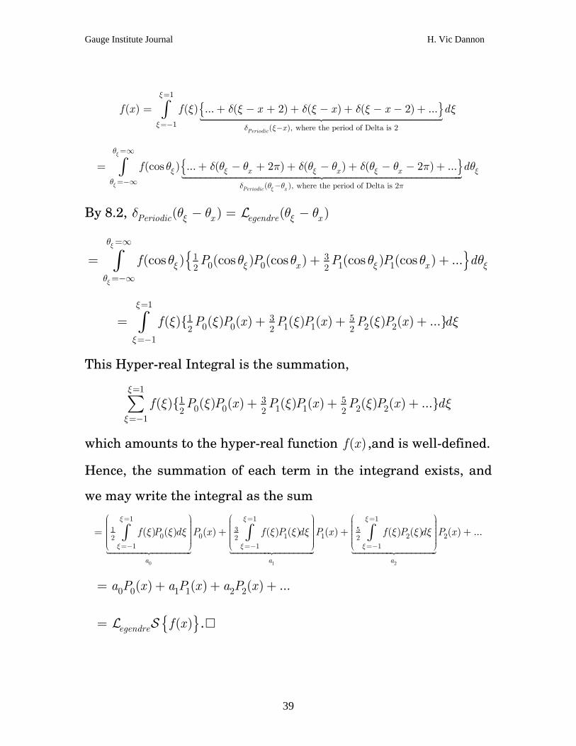
{ }1

1 ( ), where the period of Delta is 2

( ) ( ) ... ( 2) ( ) ( 2) ...

Periodic x

f x f x x x dξ

ξ δ ξ

ξ δ ξ δ ξ δ ξ=

=− −

= + − + + − + − − +∫ ξ

{ }( ), where the period of Delta is 2

(cos ) ... ( 2 ) ( ) ( 2 ) ...

Periodic x

x x xf dξ

ξξ

θ

ξ ξ ξ ξθ δ θ θ π

θ δ θ θ π δ θ θ δ θ θ π θ=∞

=−∞ −

= + − + + − + − −∫ ξ+

θ

By 8.2, ( ) ( )Periodic x egendre xξ ξδ θ θ θ− = −L

{ }1 30 0 1 12 2

(cos ) (cos ) (cos ) (cos ) (cos ) ...x xf P P P Pξ

ξ

θ

ξ ξ ξθ

θ θ θ θ θ=∞

=−∞

= +∫ d ξθ+

1

1 3 50 0 1 1 2 22 2 2

1

( ){ ( ) ( ) ( ) ( ) ( ) ( ) ...}f P P x P P x P P x dξ

ξ

ξ ξ ξ ξ=

=−

= + +∫ ξ+

This Hyper-real Integral is the summation,

11 3 5

0 0 1 1 2 22 2 21

( ){ ( ) ( ) ( ) ( ) ( ) ( ) ...}f P P x P P x P P x dξ

ξ

ξ ξ ξ ξ=

=−

+ + +∑ ξ

which amounts to the hyper-real function ( )f x ,and is well-defined.

Hence, the summation of each term in the integrand exists, and

we may write the integral as the sum

0 1 2

1 1 1

1 3 50 0 1 1 2 22 2 2

1 1 1

( ) ( ) ( ) ( ) ( ) ( ) ( ) ( ) ( ) ...

a a a

f P d P x f P d P x f P d P xξ ξ ξ

ξ ξ ξ


=− =− =−

⎛ ⎞ ⎛ ⎞ ⎛ ⎞⎟ ⎟⎜ ⎜ ⎜⎟ ⎟⎜ ⎜ ⎜⎟ ⎟= + +⎜ ⎜ ⎜⎟ ⎟⎜ ⎜ ⎜⎟ ⎟⎜ ⎜ ⎜⎟ ⎟⎝ ⎠ ⎝ ⎠ ⎝ ⎠∫ ∫ ∫

⎟⎟⎟ +⎟⎟⎟

+

0 0 1 1 2 2( ) ( ) ( ) ...a P x a P x a P x= + +

{ }( )egendre f x= L S .

39


In particular, the periodic Delta Function violates the Picone

Conditions

The Hyper-real ,is not defined in the Calculus of Limits,

and is not integrable in [ 1 .

( )xδ

,1]−

is not of bounded variation in [ 1 . 2(1 ) ( )x xδ− ,1]−

But by 9.2, satisfies the Legendre Series Theorem. ( )Periodic xδ

40


References

[Abramowitz] Abramowitz, M., and Stegun, I., “Handbook of Mathematical

Functions with Formulas Graphs and Mathematical Tables”, U.S.

Department of Commerce, National Bureau of Standards, 1964.

[Dan1] Dannon, H. Vic, “Well-Ordering of the Reals, Equality of all Infinities,

and the Continuum Hypothesis” in Gauge Institute Journal Vol. 6 No. 2, May

2010;

[Dan2] Dannon, H. Vic, “Infinitesimals” in Gauge Institute Journal Vol.6 No.

4, November 2010;

[Dan3] Dannon, H. Vic, “Infinitesimal Calculus” in Gauge Institute Journal

Vol. 7 No. 4, November 2011;

[Dan4] Dannon, H. Vic, “Riemann’s Zeta Function: the Riemann Hypothesis

Origin, the Factorization Error, and the Count of the Primes”, in Gauge

Institute Journal of Math and Physics, Vol. 5, No. 4, November 2009.

[Dan5] Dannon, H. Vic, “The Delta Function” in Gauge Institute Journal Vol.

8, No. 1, February, 2012;

[Dan6] Dannon, H. Vic, “Riemannian Trigonometric Series”, Gauge Institute

Journal, Volume 7, No. 3, August 2011.

[Dan7] Dannon, H. Vic, “Delta Function the Fourier Transform, and the

Fourier Integral Theorem” in Gauge Institute Journal Vol. 8, No. 2, May,

2012;

[Dan8] Dannon, H. Vic, “Infinite Series with Infinite Hyper-real Sum ” in

Gauge Institute Journal Vol. 8, No. 3, August, 2012;

[Ferrers] Ferrers, N., M., “An Elementary treatment on Spherical Harmonics”,

Macmillan, 1877.

41


[Gradshteyn] Gradshteyn, I., S., and Ryzhik, I., M., “Tables of Integrals Series

and Products”, 7th Edition, edited by Allan Jeffery, and Daniel Zwillinger,

Academic Press, 2007

[Hardy] Hardy, G. H., Divergent Series, Chelsea 1991.

[Hobson] Hobson, E., W., “The Theory of Spherical and Ellipsoidal

Harmonics”, Cambridge University Press, 1931.

[Jackson] Jackson, Dunham, “Fourier Series and Orthogonal Polynomials”,

Mathematical association of America, 1941.

[Sansone] Sansone, Giovanni, “Orthogonal Functions”, Revised Edition,

Krieger, 1977.

[Spiegel] Spiegel, Murray, “Mathematical Handbook of formulas and tables”

Schaum’s Outline Series, McGraw Hill, 1968.

[Szego] Szego, Gabor, “Orthogonal Polynomials” Fourth Edition, American

Mathematical Society,1975.

[Todhunter] Todhunter, I., “An Elementary Treatment on Laplace’s

Functions, Lame’s Functions, and Bessel’s Functions” Macmillan, 1875.

[Weisstein], Weisstein, Eric, W., “CRC Encyclopedia of Mathematics”, Third

Edition, CRC Press, 2009.

42

periodic delta function and expansion in legendre polynomials

Documents