new operational matrix for shifted legendre …pu.edu.pk/images/journal/maths/pdf/9_4-02-09.pdfnew...

Punjab UniversityJournal of Mathematics (ISSN 1016-2526)Vol.47(1)(2015) pp.00.00

New Operational Matrix For Shifted Legendre Polynomials and FractionalDifferential Equations With Variable Coefficients

Hammad KhalilDepartment of Mathematics,

University of Malakand , KPK, Pakistanemail: [email protected]

Rahmat Ali KhanDepartment of Mathematics,

University of Malakand , KPK, Pakistanemail: [email protected]

Mohammed H. Al-SmadiApplied Science Department, Ajloun College

Al- Balqa Applied University, Ajloun 26826, Jordanemail: [email protected]

Asad A. FreihatPioneer Center for Gifted Students,

Ministry of Education, Jerash 26110 Jordan .email: [email protected]

Nabil ShawagfehDepartment of Mathematics,University of Jordan

Received: 17 February, 2015 / Accepted: 15 April, 2015 / Published online: 23 April, 2015

Abstract. This paper is devoted to study a computation scheme to ap-proximate solution of fractional differential equations(FDEs) and coupledsystem of FDEs with variable coefficients. We study some interestingproperties of shifted Legendre polynomials and develop a new operationalmatrix. The new matrix is used along with some previously derived re-sults to provide a theoretical treatment to approximate the solution of ageneralized class of FDEs with variable coefficients. The new methodhave ability to convert fractional order differential equations having vari-able coefficients to system of easily solvable algebraic equations. Wegave some details to show the convergence of the scheme. The efficiencyand applicability of the method is shown by solving some test problems.To show high accuracy of proposed method we compare out results with

1

2 H. Khalil

some other results available in the literature. The proposed method iscomputer oriented. We useMatLab to carry out necessary calculations.

AMS (MOS) Subject Classification Codes: 65N35; 65M70; 35C11Key Words: Legendre polynomials; Approximation theory; Fractional differential equa-

tions.

1. INTRODUCTION

In recent years considerable interest in fractional differential equations (FDE) has beenstimulated due to their numerous applications in the areas of physics and engineering seefor example [36, 33, 21, 28]. After the discovery of fractional calculus ( derivative andintegral of non integer order) it is shown that fractional order differential equations (FDEs)can provide a more real insight in the phenomena as compared to the ordinary differentialequations (see for example [23]). The exact analytic solution of FDEs is available only fora considerable small class of FDEs. Some time it is very difficult to obtain the exact ana-lytic solutions of fractional differential equations. In some cases it becomes impossible toarrive at the exact analytic solution. The reason of this difficulty is the great computationalcomplexities of fractional calculus involving in these equations.

This paper deals with the approximate solution of generalized classes of multi termfractional differential equations with variable coefficients of the form

∂σU(t)∂tσ

=a∑

i=0

φi(t)∂iU(t)

∂ti+ f(t), (1. 1)

with initial conditionsU i(0) = ui, i = 0, 1, · · · a.

Whereui are all real constants,a < σ ≤ a + 1, t ∈ [0, τ ], U(t) is the unknown solutionto be determined,f(t) is the given source term andφi(t) for i = 0, 1 · · · a are coefficientsdepends ont and are well defined on[0, τ ].

∂σU(t)∂tσ

=n∑

i=0

φi(t)∂iU(t)

∂ti+

n∑

i=0

ψi(t)∂iV (t)

∂ti+ f(t),

∂σV (t))∂tσ

=n∑

i=0

ϕi(t)∂iU(t)

∂ti+

n∑

i=0

%i(t)∂iV (t)

∂ti+ g(t),

(1. 2)

with initial conditions

U i(0) = ui, i = 0, 1, 2 · · ·n,

V i(0) = vi, i = 0, 1, 2 · · ·n.

Heren < σ ≤ n + 1, ui andvi are real constants,φi(t), ψi(t), ϕi(t) and %i(t) are givenvariable coefficients and are continuously differentiable and well defined on[0, τ ]. U(t)andV (t) are the unknown solutions to be determined whilef(t) andg(t) are the givensource terms.

Many important differential equations which are of basic importance especially in mod-eling the real world problems belong generalized class of differential equations defined in(1. 1 ) see for example [28, 22, 34]. In [23] A. Monje, use such type of differential equa-tions to model behavior of immersed plate in fluid. In [28]PDν−controler is modeled

New Operational Matrix For Shifted Legendre Polynomials and Fractional Differential Equations With Variable Coefficients. 3

using such types of equations and it is shown that using fractional order differential equa-tions we can get a more real insight in the phenomena as compared to the ordinary case.

Many authors existence of solution of such problems. Among others Yi Chen et al [2]study the existence results of the solution of the problem and provide sufficient conditionsunder which the solution of the problem exists. They use Leggett-Williams fixed pointtheorem to prove the existence of positive solutions of the corresponding problems. Inthis paper we assume thatU(t) satisfy all the necessary conditions for existence of uniquesolution.

Various attempts were made to approximate solution of such type of problems. YildirayKeskin [10] proposed a new technique based of generalized Taylor polynomials for the nu-merical solution of such types of equations. In [25, 38] an approach is made to approximatesolution of such problems, their approach is based on rationalized Chebeshev polynomi-als combined with tau method. In [37] the author use collocation approach to solve suchtype of problems. In [29] the author study improve Chebeshev collocation method forsolution of such problems. More recently J. Liu et al [20] use the Legendre spectral Taumethod to obtain the solution of fractional order partial differential equations with variablecoefficients. Kilbas et al [17], investigate solutions around an ordinary point for linear ho-mogeneous Caputo fractional differential equations with sequential fractional derivativesof orderkα(0 < α = 1) having variable coefficients. In [18], the authors studied onexplicit representations of Greens function for linear (Riemann-Liouvilles) fractional dif-ferential operators with variable coefficients continuous in[0,∞) and applied it to obtainexplicit representations for solution of non-homogeneous fractional differential equationwith variable coefficients of general type.

Recently the operational matrix method got attention of many mathematicians. Thereason is high simplicity and efficiency of the method. Different kinds of differentialand partial differential equations are efficiently solved using this method see for exam-ple [?, 35, 26, 3, 4, 5,?, ?, 11, 12, 13] and the references quoted there. The operationalmatrix method is based on various orthogonal polynomials and wavelets. A deep insight inthe method shows that the method is really very simple and accurate. But up to know to thebest of our knowledge the method is only used to find the approximate solution of differen-tial equations, partial differential equation (including fractional order) only with constantcoefficients. Up to know this method is not able to solve fractional differential equationswith variable coefficients, due to non availability of necessary operational matrices.

We generalize the operational matrix method to solve fractional differential equationswith variable coefficients. We develop some new operational matrices. These new matricesare used to convert the generalize class of FDEs to a system of easily solvable algebraicequations. We also apply the new matrices to solve coupled system of FDEs with variablecoefficients. For detailed study on spectral approximation and fractional calculus we referthe reader to studies [14, 7, 19].

The rest of the article is organized as follows : In section2, we provide some prelimi-naries of fractional calculus, Legendre polynomials and some basic results from approxi-mation theory. In section3, we recall some other operational matrices of integration anddifferentiation for shifted Legendre polynomials and derive some new operational matri-ces. In section4 operational matrices are used to establish a new scheme for solution of ageneralized class of FDEs with variable coefficients and coupled FDEs with variable coef-ficients. In section5 the we derive some relation for convergence of proposed method and

4 H. Khalil

obtain some upper bound for the error of approximate solution. In section6, some numer-ical experiments is performed to show the efficiency of the new technique. And finally insection7 a short conclusions is made.

2. PRELIMINARIES

In this section we recall some basic definitions and concepts from open literature whichare of basic importance in further development in this paper.

Definition 1: [27, 16]According to Riemann-Liouville the fractional order integral oforderα ∈ R+ of a functionφ ∈ (L1[a, b],R) on interval[a, b] ⊂ R, is defined by

Iαa+φ(x) =

1Γ (α)

∫ x

a

(x− s)α−1φ(s)ds, (2. 3)

provided that the integral on right hand side exists.Definition 2: For a given functionφ(t) ∈ Cn[a, b], the Caputo fractional order deriva-

tive of orderα is defined as

Dαφ(x) =1

Γ(n− α)

∫ x

a

φ(n)(s)(x− s)α+1−n

ds, n− 1 ≤ α < n , n ∈ N, (2. 4)

provided that the right side is point wise defined on(a,∞), wheren = [α] + 1.From (2. 3 ),(2. 4 ) it is easily deduced that

Dαxk =Γ(1 + k)

Γ(1 + k − α)xk−α, Iαxk =

Γ(1 + k)Γ(1 + k + α)

xk+α and DαC = 0, for a constantC.

(2. 5)

2.1. The shifted Legendre polynomials: The Legendre polynomials defined on[−1, 1]are given by the following recurrence relation (see [13])

Li+1(z) =2i + 1i + 1

zLi(z)− i

i + 1Li−1(z), i = 1, 2.... whereL0(z) = 0, L1(z) = z.

The transformationt = τ(z+1)2 transforms the interval[−1, 1] to [0, τ ] and the shifted

Legendre polynomials are given by

Lτi (t) =

i∑

k=0

,i,ktkג i = 0, 1, 2, 3..., (2. 6)

(i,k)ג =(−1)i+k(i + k)!(i− k)!τk(k!)2

. (2. 7)

These polynomials are orthogonal and the orthogonality condition is∫ τ

0

Lτi (t)Lτ

j (t)dt ={

τ2i+1 , if i = j,

0, if i 6= j.(2. 8)

By the use of orthogonality condition (2. 8 ) anyf(t) ∈ C([0, τ ]) can be approximatedwith Legendre polynomials ie

f(t) ≈m∑

l=0

clLτl (t), where cl =

(2l + 1)τ

∫ τ

0

f(t)Lτl (t)dt. (2. 9)

As l →∞ the approximation becomes equal to the exact function.


In vector notation, we write

f(t) ≈ CTMΛτ

M (t), (2. 10)

where

ΛτM (t) =

[Lτ

0(t) Lτ1(t) · · · Lτ

i (t) · · · Lτm(t)

]T(2. 11)

and

CM =[

c0 c1 · · · ci · · · cm

]T. (2. 12)

M = m + 1 is the scale level of the approximation.The following lemma is very important for our further analysis.

LEMMA 2.1. The definite integral of product of any three Legendre polynomials on thedomain[0, τ ] is a constant and the value of that constant is♥(i,j,k)

(l,m,n) ie∫ τ

0

Lτi (t)Lτ

j (t)Lτk(t)dt = ♥(i,j,k)

(l,m,n), (2. 13)

where

♥(i,j,k)(l,m,n) =

i∑

l=0

j∑m=0

k∑n=0

.Υ(l,m,n)(i,n)ג(i,m)ג(i,l)ג

(.,.)ג are as defined in(2. 7 )and

Υ(l,m,n) =τ (l+m+n+1)

(l + m + n + 1).

Proof. The proof of this lemma is straight forward.Consider

∫ τ

0

Lτi (t)Lτ

j (t)Lτk(t)dt =

i∑

l=0

(i,l)גj∑

m=0

(j,m)ג

k∑n=0

(k,n)ג

∫ τ

0

t(l+m+n)dt. (2. 14)

The integral in the above equation is equal to∫ τ

0

t(l+m+n)dt =τ (l+m+n+1)

(l + m + n + 1). (2. 15)

ConsiderΥ(l,m,n) = τ(l+m+n+1)

(l+m+n+1) . Then

∫ τ

0

Lτi (t)Lτ

j (t)Lτk(t)dt =

i∑

l=0

j∑m=0

k∑n=0

.Υ(l,m,n)(k,n)ג(j,m)ג(i,l)ג (2. 16)

Let suppose

♥(i,j,k)(l,m,n) =

i∑

l=0

j∑m=0

k∑n=0

.Υ(l,m,n)(k,n)ג(j,m)ג(i,l)ג (2. 17)

And hence the proof is complete. ¤

The constant defined in the above lemma plays (very)important role in the developmentof the new matrix.

The following theorem is important for the convergence of the scheme.

6 H. Khalil

THEOREM 2.1. Let∏

M be the space ofM terms Legendre polynomials and letu(t) ∈Cm[0, 1], thenum(t) is in space

∏M . Then we have

u(t) =m∑

i=0

ciLτi (t), (2. 18)

then

ck ' C

λk

m

‖u(m)‖. (2. 19)

and

‖u(t)−m∑

i=0

ciLτi (t)‖2 ≤

∞∑

k=m+1

λkc2k, (2. 20)

where

ck =2k + 1

τ

∫ τ

0

u(t)Lτk(t)dt, λk = k(k + 1). (2. 21)

C is constant and can be chosen in such a way thatu(2m) belong to∏

M . Whereu(m)

is defined as

u(m) = L(u(m−1)) = Lm(u(0)) (2. 22)

whereL is storm livoli operator of legendre polynomials withu(0) = u(t).

Proof. Proof of this theorem is analogous as in [13] and references therein. ¤

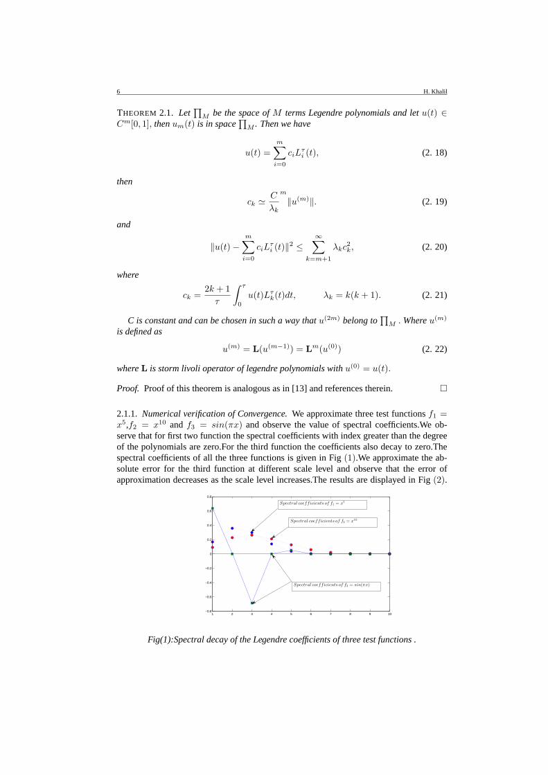
2.1.1. Numerical verification of Convergence.We approximate three test functionsf1 =x5,f2 = x10 and f3 = sin(πx) and observe the value of spectral coefficients.We ob-serve that for first two function the spectral coefficients with index greater than the degreeof the polynomials are zero.For the third function the coefficients also decay to zero.Thespectral coefficients of all the three functions is given in Fig(1).We approximate the ab-solute error for the third function at different scale level and observe that the error ofapproximation decreases as the scale level increases.The results are displayed in Fig(2).

1 2 3 4 5 6 7 8 9 10−0.8

−0.6

−0.4

−0.2

0

0.2

0.4

0.6

0.8

Spectral coefficients of f3 = sin(πx)

Spectral coefficients of f1 = x5

Spectral coefficients of f2 = x10

Fig(1):Spectral decay of the Legendre coefficients of three test functions .


0 0.5 1

0

1

2

3

4

5

6

7

8

x 10−4

x

0 0.5 1

0

1

2

3

4

5

6

7

8

9

x 10−6

x

0 0.5 1

0

1

2

3

4

5

6

x 10−8

x

Error at M=9Error at M=8Error at M=7

Fig(2):Absolute amount of error forf3 = sin(πx) at different scale level.

It is concluded that the Legendre polynomials provide a good approximation to continuousfunction.The error of approximation decreases rapidly with the increase of scale level.Forexample (Fig(2) )the error is less than10−4 at scale level M=7 and as we increase thescale level the error is less than10−6 and10−8.

3. MAIN RESULT:NEW OPERATIONAL MATRIX

First of all we recall some existent results which are of basic importance in the formu-lation of our result.

LEMMA 3.1. let ΛτM (t) be the function vector as defined in(2. 11 )then the integration of

orderα of ΛτM (t) is generalized as

Iα(ΛτM (t)) ' Hτ,α

M×MΛτM (t), (3. 23)

whereHτ,αM×M is the operational matrix of integration of orderα and is defined as

Hτ,αM×M =

Θ0,0,τ Θ0,1,τ · · · Θ0,j,τ · · · Θ0,m,τ

Θ1,0,τ Θ1,1,τ · · · Θ1,j,τ · · · Θ1,m,τ

......

......

......

Θi,0,τ Θi,1,τ · · · Θi,j,τ · · · Θi,m,τ

......

......

......

Θm,0,τ Θm,1,τ · · · Θm,j,τ · · · Θm,m,τ

, (3. 24)

where

Θi,j,τ =i∑

k=0

sk,jגi,kΓ(k + 1)

Γ(k + α + 1). (3. 25)

Alsoגi,k is similar as defined in(2. 7 )and

sk,j =(2j + 1)

τ

j∑

l=0

(−1)j+l(j + l)!(τ)k+l+α+1

(τ l)(j − l)(l!)2(k + l + α + 1). (3. 26)

8 H. Khalil

Proof. Using (2. 5 ) along with (2. 6 ) we have

IαLτi (t) =

i∑

k=0

i,kIαtkג

=i∑

k=0

i,kגΓ(k + 1)

Γ(k + α + 1)tk+α.

(3. 27)

Approximatingtk+α with m + 1 terms of Legendre polynomial we get

tk+α 'm∑

j=0

sk,jLτj (t), (3. 28)

we can easily calculate the value ofsk,j by using the orthogonality condition ie

sk,j =(2j + 1)

τ

j∑

l=0

(−1)j+l(j + l)!(τ)k+l+α+1

(τ l)(j − l)(l!)2(k + l + α + 1). (3. 29)

Employing (3. 27 ), and (3. 29 ) we get

IαLτi (t) =

m∑

j=0

i∑

k=0

sk,jגi,kΓ(k + 1)

Γ(k + α + 1)Lτ

j (t).

Setting

Θi,j,τ =i∑

k=0

sk,jגi,kΓ(k + 1)

Γ(k + α + 1), (3. 30)

we get

IαLτi (t) =

m∑

j=0

Θi,j,τLτj (t), (3. 31)

or evaluating for differenti we get the desired result. ¤

Corollary 1: The error |EM | = |IαU(t) − KTMHτ,α

M×MΛτM (t)| in approximating

IαU(t) with operational matrix of fractional integration is bounded by the following.

|EM | ≤ |∞∑

k=m+1

ck{m∑

i=0

Θi,j,τ}|. (3. 32)

Proof. Consider

U(t) =∞∑

k=0

ckLτk(t). (3. 33)

Then using relation (3. 31 ) we get

IαU(t) =∞∑

k=0

ck

m∑

j=0

Θk,j,τLτj (t). (3. 34)

Truncating the sum and writing in modified form we get

IαU(t)−m∑

k=0

ck

m∑

j=0

Θk,j,τLτj (t) =

∞∑

k=m+1

ck

m∑

j=0

Θk,j,τLτj (t). (3. 35)


We can also write it in matrix form as

IαU(t)−KTMHτ,α

M×MΛτM (t) =

∞∑

k=m+1

ck

m∑

j=0

Θk,j,τLτj (t). (3. 36)

But Lτj (t) ≤ 1 for t ∈ [0, 1] therefore we can write

|IαU(t)−KTMHτ,α

M×MΛτM (t)| ≤ |

∞∑

k=m+1

ck

m∑

j=0

Θk,j,τ |. (3. 37)


LEMMA 3.2. let ΛτM (t) be the function vector as defined in(2. 11 )then the derivative of

orderα of ΛτM (t) is generalized as

Dα(ΛτM (t)) ' Gτ,α

M×MΛτM (t), (3. 38)

whereGτ,αM×M is the operational matrix of derivatives of orderα and is defined as

Gτ,αM×M =

Φ0,0,τ Φ0,1,τ · · · Φ0,j,τ · · · Φ0,m,τ

Φ1,0,τ Φ1,1,τ · · · Φ1,j,τ · · · Φ1,m,τ

......

......

......

Φi,0,τ Φi,1,τ · · · Φi,j,τ · · · Φi,m,τ

......

......

......

Φm,0,τ Φm,1,τ · · · Φm,j,τ · · · Φm,m,τ

. (3. 39)

Where

Φi,j,τ =i∑

k=dαesk,jגi,k

Γ(k + 1)Γ(k − α + 1)

, (3. 40)

with Φi,j,τ = 0 if i < dαe. Alsoגi,k is similar as defined in(2. 7 )and

sk,j =(2j + 1)

τ

j∑

l=0

(−1)j+l(j + l)!(τ)k+l−α+1

(τ l)(j − l)(l!)2(k + l − α + 1). (3. 41)

Proof. The proof of this lemma is similar as above Lemma. ¤

Corollary 2: The error|EM | = |DαU(t) − KTMGτ,α

M×MΛτM (t)| in approximating

DαU(t) with operational matrix of derivative is bounded by the following.

|EM | ≤ |∞∑

k=m+1

ck{m∑

i=dαeΦi,j,τ}| (3. 42)

Proof. The proof of this corollary is similar as Corollary 1. ¤

LEMMA 3.3. LetU(t) andφn(t) be any function defined on[0, τ ]. Then

φn(t)∂σU(t)

∂tσ= WT

MQσφn

ΛτM (t). (3. 43)

WhereWTM is the Legendre coefficient vector ofU(t) as defined in(2. 10 )and

Qσφn

= Gτ,σM×MRτ,φn

M×M . (3. 44)

The matrixGτ,σM×M (defined in Lemma 3.2) is the operational matrix of derivative of order

σ and

10 H. Khalil

Rτ,φn

M×M =

Θ0,0 Θ0,1 · · · Θ0,s · · · Θ0,m

Θ1,0 Θ1,1 · · · Θ1,s · · · Θ1,m

......

......

......

Θr,0 Θr,1 · · · Θr,s · · · Θr,m

......

......

. .....

Θm,0 Θm,1 · · · Θm,s · · · Θm,m

. (3. 45)

Where

Θr,s =2s + 1

τ

m∑

i=0

ci♥(i,r,s)(l,m′,n). (3. 46)

Whereci =∫ τ

0φn(t)Lτ

i (t)dt, and♥(i,r,s)(l,m′,n) is as defined in Lemma 2.2.1.

Proof. ConsiderU(t) ' WTMΛτ

M (t), then by use of Lemma 3.2 we can easily write

φn(t)∂σU(t)

∂tσ= φn(t)WT

MGτ,σM×MΛτ

M (t). (3. 47)

The above equation can also be written in the following form

φn(t)∂σU(t)

∂tσ= WT

MGτ,σM×M

︷︸︸︷Λτ

M (t) . (3. 48)

Where︷︸︸︷Λτ

M (t) =[

φn(t)Lτ0(t) φn(t)Lτ

1(t) · · · φn(t)Lτi (t) · · · φn(t)Lτ

m(t)]T

.(3. 49)

Approximatingφn(t) with M terms of Legendre polynomials we get

φn(t) 'm∑

i=0

ciLτi (t). (3. 50)

Using (3. 50 ) in (3. 49 ) we can get︷︸︸︷Λτ

M (t) =[ ℵ0(t) ℵ1(t) · · · ℵr(t) · · · ℵm(t)

]T, (3. 51)

where

ℵr(t) =m∑

i=0

ciLτi (t)Lτ

r (t) , r = 0, 1 · · ·m. (3. 52)

We can approximate the general termℵr(t) with M terms of Legendre polynomials asfollows

ℵr(t) =m∑

s=0

hrsL

τs (t), (3. 53)

where

hrs =

2s + 1τ

∫ τ

0

ℵr(t)Lτs (t)dt. (3. 54)

Using (3. 52 ) in (3. 54 ) we get

hrs =

2s + 1τ

m∑

i=0

ci

∫ τ

0

Lτi (t)Lτ

r (t)Lτs (t)dt. (3. 55)


Know using lemma 2.1 and (3. 55 ) we get

hrs =

2s + 1τ

m∑

i=0

ci♥(i,r,s)(l,m′,n). (3. 56)

Let suppose

Θr,s =2s + 1

τ

m∑

i=0

ci♥(i,r,s)(l,m′,n). (3. 57)

Then repeating the procedure forr = 0, 1, · · ·m ands = 0, 1, · · ·m we can write

ℵ0(t)ℵ1(t)· · ·ℵr(t)· · ·ℵm(t)

=

Θ0,0 Θ0,1 · · · Θ0,s · · · Θ0,m

Θ1,0 Θ1,1 · · · Θ1,s · · · Θ1,m

......

......

......

Θr,0 Θr,1 · · · Θr,s · · · Θr,m

......

......

. . ....

Θm,0 Θm,1 · · · Θm,s · · · Θm,m

Lτ0(t)

Lτ1(t)...

Lτs (t)...

Lτm(t)

. (3. 58)

We may write the above equation as︷︸︸︷Λτ

M (t) = Rτ,φn

M×MΛτM (t). (3. 59)

Using (3. 59 ) in (3. 48 ) we get

φn(t)∂σU(t)

∂tσ= WT

MGτ,σM×MRτ,φn

M×MΛτM (t). (3. 60)

Let Gτ,σM×MRτ,φn

M×M = Qσφn

. Then we have

φn(t)∂σU(t)

∂tσ= WT

MQσφn

ΛτM (t). (3. 61)


4. APPLICATION OF THE NEW MATRIX

In this section we apply the new matrix to approximate the solution of fractional orderdifferential equations.

4.1. FDEs with variable equations. Consider the following generalized class of FDEswith variable coefficients

∂σU(t)∂tσ

=n∑

i=0

φi(t)∂iU(t)

∂ti+ f(t), (4. 62)

subject to initial conditions

U i(0) = ui, i = 0, 1, · · ·n.

Whereui are all real constant,n < σ ≤ n + 1, t ∈ [0, τ ], U(t) is the unknown solution tobe determined,f(t) is the given source term andφi(t) for i = 0, 1 · · ·n are coefficientsdepends ont and are well defined on[0, τ ]. The solution of the above problem can bewritten in terms of shifted Legendre series such that

∂σU(t)∂tσ

= WTMΛτ

M (t). (4. 63)

12 H. Khalil

Applying fractional integral of orderσ and by using the given initial conditions we get

U(t)−n∑

j=0

tjuj = WTMHτ,σ

M×MΛτM (t). (4. 64)

Which can be simplified as

U(t) = WTMHτ,σ

M×MΛτM (t) + FT

1 ΛτM (t), (4. 65)

whereFT1 Λτ

M (t) =∑n

j=0 tjuj . We can also write it as

U(t) = WTMΛτ

M (t), (4. 66)

whereWT

M = WTMHη,σ

M×M + FT1 . (4. 67)

Using (4. 66 ) along with Lemma 3.3 we can write

φi(t)∂iU(t)

∂ti= WT

MQiφi

ΛτM (t). (4. 68)

Approximatingf(t) = F2ΛτM (t) and using (4. 68 ) in (4. 62 ) we get

WTMΛτ

M (t) =n∑

i=0

WTMQi

φiΛτ

M (t) + F2ΛτM (t). (4. 69)

On further simplification we get

{WTM − WT

M

n∑

i=0

Qiφi− F2}Λτ

M (t) = 0. (4. 70)

Or

{WTM − WT

M

n∑

i=0

Qiφi− F2} = 0. (4. 71)

Now using (4. 67 ) we can write the above equation as

{WTM −WT

M

n∑

i=0

Hη,σM×MQi

φi−

n∑

i=0

F1Qiφi− F2} = 0. (4. 72)

Equation (4. 72 ) is easily solvable algebraic equation and can be easily solved for theunknown coefficient vectorWT

M .Using the value ofWTM in equation (4. 65 ) will arrive us

to the approximate solution of the problem.

4.2. Coupled system of FDEs with variable equations.The Q-Matrix is also helpfulwhen we want to approximate the solution of coupled system of fractional order differentialequations having variable coefficients. Consider the generalize class of system

∂σU(t)∂tσ

=n∑

i=0

φi(t)∂iU(t)

∂ti+

n∑

i=0

ψi(t)∂iV (t)

∂ti+ f(t),

∂σV (t))∂tσ

=n∑

i=0

ϕi(t)∂iU(t)

∂ti+

n∑

i=0

%i(t)∂iV (t)

∂ti+ g(t),

(4. 73)

with initial conditions

U i(0) = ui, i = 0, 1, 2 · · ·n,

V i(0) = vi, i = 0, 1, 2 · · ·n.


Heren < σ ≤ n + 1, ui andvi are real constants,φi(t), ψi(t), ϕi(t) and %i(t) are givenvariable coefficients and are continuously differentiable and well defined on[0, τ ]. U(t)andV (t) are the unknown solutions to be determined whilef(t) andg(t) are the givensource terms. We seek the solutions of above equations in terms of shifted Legendre poly-nomials such that

∂σU(t)∂tσ

= WTMΛτ

M (t),∂σZ(x)

∂xσ= ET

MΛτM (t). (4. 74)

By the application of fractional integration of orderσ on both equations and using initialconditions allows us to write (4. 74 ) as

U(t) = WTMΛτ

M (t), V (t) = ETMΛτ

M (t). (4. 75)

Where

WTM = WT

MHτ,σM×M + FT

1 , ETM = ET

MHτ,σM×M + FT

2 . (4. 76)

Note here thatFT1 Λτ

M (t) =∑n

i=0 uiti and FT

2 ΛτM (t) =

∑ni=0 vit

i. Using equation(4. 75 ) along with Lemma 3.3 we may write

n∑

i=0

φi(t)∂iU(t)

∂ti= WT

M

n∑

i=0

Qiφi

ΛτM (t),

n∑

i=0

ψi(t)∂iV (t)

∂ti= ET

M

n∑

i=0

Qiψi

ΛτM (t),

n∑

i=0

ϕi(t)∂iU(t)

∂ti= WT

M

n∑

i=0

Qiϕi

ΛτM (t),

n∑

i=0

%i(t)∂iV (t)

∂ti= ET

M

n∑

i=0

Qi%i

ΛτM (t).

(4. 77)

Approximating the source termsf(t) and g(t) with shifted Legendre polynomials andusing (4. 77 ),(4. 74 ) in (4. 73 ) and writing in vector notation we get

[WT

MΛτM (t)

ETMΛτ

M (t)

]=

[WT

M

∑ni=0 Qi

φiΛτ

M (t)ET

M

∑ni=0 Qi

%iΛτ

M (t)

]+

[ET

M

∑ni=0 Qi

ψiΛτ

M (t)WT

M

∑ni=0 Qi

ϕiΛτ

M (t)

]+

[FMΛτ

M (t)GMΛτ

M (t)

].

(4. 78)

By taking the transpose of the (4. 78 ) and after a short manipulation we get

[WT

M ETM

]A =

[WT

M ETM

] [ ∑ni=0 Qi

φiOM×M

OM×M

∑ni=0 Qi

%i

]A

+[

WTM ET

M

] [OM×M

∑ni=0 Qi

ϕi∑ni=0 Qi

ψiOM×M

]A +

[FM GM

]A.

(4. 79)

WhereA =[

ΛτM (t) OM

OM ΛτM (t))

], OM andOM×M is zero vector and zero matrix of

orderM respectively. Canceling out the common terms and after a short simplification weget

[WT

M ETM

]− [WT

M ETM

] [ ∑ni=0 Qi

φi

∑ni=0 Qi

ϕi∑ni=0 Qi

ψi

∑ni=0 Qi

%i

]− [

FM GM

]= 0.

(4. 80)

14 H. Khalil

Using (4. 76 ) in (4. 80 ) we get

[WT

M ETM

]− [WT

M ETM

] [Hτ,σ

M×M

∑ni=0 Qi

φiHτ,σ

M×M

∑ni=0 Qi

ϕi

Hτ,σM×M

∑ni=0 Qi

ψiHτ,σ

M×M

∑ni=0 Qi

%i

]

− [FT

1 FT2

] [ ∑ni=0 Qi

φi

∑ni=0 Qi

ϕi∑ni=0 Qi

ψi

∑ni=0 Qi

%i

]− [

FM GM

]= 0.

Which is easily solvable generalized sylvester type matrix equation and can be easilysolved for the unknown

[WT

M ETM

]. Using these values in (4. 75 ) along with (4. 76 )

will lead us to the approximate solutions to the problem.

5. ERROR BOUND OF THE APPROXIMATE SOLUTION

In this section we calculate a bound for error of approximation of solution with theproposed method. From Lemma 2.2 we conclude that Legendre polynomials are wellsuited to approximate a sufficiently continuous function on the bounded domain. We canalso see thatck → 0 faster than any algebraic sequence ofλk. Which means that as thescale level increase coefficients decreases and approaches to zero. Consider the followingfractional differential equation.

∂σU(t)∂tσ

=n∑

i=0

φi(t)∂iU(t)

∂ti+ f(t), (5. 81)

Our aim is to derive upper bound for proposed method. We have to calculate|E1M | defined

as

|E1M | = |∂

σU(t)∂tσ

−KTMΛτ

M (t)|. (5. 82)

As in previous section we initially assume the highest derivative in terms of legender poly-nomials and then we use operational matrices to convert differential equation to system ofalgebraic equations. In last we get the initial assumption we made and then using opera-tional matrix of integration we get the approximate solution. Therefore to obtain the upperbound for approximate solution we follow the same route.

Consider the following generalized class of FDEs with variable coefficients

∂σU(t)∂tσ

=n∑

i=0

φi(t)∂iU(t)

∂ti+ f(t), (5. 83)

subject to initial conditions

U i(0) = ui, i = 0, 1, · · ·n.

The solution of the above problem can be written in terms of shifted Legendre series suchthat

∂σU(t)∂tσ

= WTMΛτ

M (t) +∞∑

k=m+1

ckLτk(t). (5. 84)

Applying fractional integral of orderσ, using operational matrix of integration and usingcorollary 1 we can write

U(t)−n∑

j=0

tjuj = WTMHτ,σ

M×MΛτM (t) +

∞∑

k=m+1

ck

m∑

i=0

Θi,k,τLτk(t). (5. 85)


Which can be simplified as

U(t) = WTMHτ,σ

M×MΛτM (t) + FT

1 ΛτM (t) +

∞∑

k=m+1

ck

m∑

i=0

Θi,k,τLτk(t), (5. 86)

Assume as in section 4.1W = WTMHτ,σ

M×M + FT1

Using Lemma 3.3 and Corollary 2 we may write we can write

φi(t)∂iU(t)

∂ti= WT

MQiφi

ΛτM (t) + φi(t)

∞∑

k=m+1

ck

m∑

i=0

m∑

i′=0

Θi,k,τΦi′,k,τLτk(t). (5. 87)

Approximatingf(t) = F2ΛτM (t) +

∑∞k′=m+1 fkLτ

k(t) and using (5. 87 ) in (5. 83 ) weget

WTMΛτ

M (t)−n∑

i=0

WTMQi

φiΛτ

M (t)− F2ΛτM (t) = RM (t). (5. 88)

WhereRM (t) is defined by relation

RM (t) =∞∑

k=m+1

ck

m∑

i=0

m∑

i′=0

Θi,k,τΦi′,k,τ

n∑s=0

φsLτs (t)(t)Lτ

k(t)

−∞∑

k=m+1

ckLτk(t) +

∞∑

k′=m+1

fkLτk(t)

(5. 89)

The proposed scheme works under assumption (see section 4.1) thatRM (t) = 0. Nowas we observe thatLτ

k(t) ≤ 1 for t ∈ [0, τ ] therefore using this property of Legendrepolynomials we get upper bound of approximate solution as

|RM | ≤∞∑

k=m+1

|ck

m∑

i=0

m∑

i′=0

n∑s=0

Θi,k,τΦi′,k,τφs −∞∑

k=m+1

ck +∞∑

k′=m+1

fk| (5. 90)

In view of Theorem 2.1 we see thatck decays to zero, as the index of truncation in-creases. Therefore it is evident that proposed algorithm converges to the approximatesolution as we increase the scale level. Using the similar procedure we may also obtainthe upper bound for error of approximation of coupled system of fractional differentialequations. As the proof is analogous therefore we skip it and proceed to further analysis.

6. TEST PROBLEMS

To show the efficiency and applicability of proposed method, we solve some test prob-lems. Where possible we compare our results with some of results available. For illustra-tion purpose we show results graphically.

Example 1: Consider the following fractional differential equation

∂σU(t)∂tσ

= et ∂U(t)∂t

+ cos (t)U(t) + F (t), (6. 91)

with initial conditionU(0) = 0 andU ′(0) = π.Where1 < σ ≤ 2, t ∈ [0, 3] and the source term is defines as

F (t) = e−tsin(πt)(1− π2)− e−tcos(πt)(sin(πt) + 2π) + sin(πt)− πcos(πt).

16 H. Khalil

The solution of this problem atσ = 2 is Y (t) = e−tsin(πt). However solution atfractional value ofσ is not known. It is well known that solution of fractional differentialequations approaches to solution of classical integer order differential equation as the or-der of derivative approaches from fractional to integer. Using this property of fractionaldifferential equations we show that the solution of our problem approaches to solution atσ = 1 asσ → 2.

At first we fix σ = 2 and approximate the solution at different scale level. We observethat the accuracy of the solution depends solely on scale level. As scale levelM increasesthe solution become more and more accurate. Fig (3) shows the comparison of exactsolution with approximate solution at different scale level.One can easily see that at scalelevel M = 8, the approximate solution just matches the exact solution. One can seefrom Fig (5) that the absolute amount of error decrease as the scale level increases and atM = 8 the error is much more less that10−2. Which is much more acceptable numberfor such hard problems. We also approximate the solution at some fractional value ofσand observe that asσ → 2 (see Fig (4))the solution approaches to the exact solution atσ = 2. Which guarantees the accuracy of the scheme for fractional differential equations.

0 0.5 1 1.5 2 2.5−0.3

−0.2

−0.1

0

0.1

0.2

0.3

0.4

0.5

0.6

0.7

t

GreenDotsExact U (t)

Approximate U (t)atM = 7


Fig(3):Comparison of exact and approximate solution of example1 at scale levelM = 7, 8.The Dots represents the exact solutions while the lines represents the

approximate solutions.

0.5 1 1.5 2 2.5−2

−1.5

−1

−0.5

0

0.5

1

1.5

x

σ = 1.5

σ = 1.6

σ = 1.7

σ = 1.8

σ = 1.9

σ = 2.0

Exact U (t)


Fig(4):Approximate solution of example 1 at fractional value ofσ and its comparisonwith the exact solution atσ = 2.The red dots represents the exact solution atσ = 2.

0 0.5 1 1.5 2 2.50

0.005

0.01

0.015

0.02

0.025

0.03

0.035

0.04

0.045

0.05

x

Absolute error inU(t)atM = 7

Absolut error inU(t)atM = 8

Fig(5):Absolute error in U(t) of example 1 at different scale level ieM = 7 andM = 8.

Example 2:As a second example we solve the following integer order differential equation [29].

D2U(t) + 2tDU(T ) = 0,

U(0) = 0, U ′(0) =2√π

.(6. 92)

The exact solution of the problem isU(t) = 2√π

∫ t

0e−x2

dx. We approximate solution tothis problem using different scale level. And observe that the approximate solution veryaccurate. The comparison of exact solution with the solution obtained with this methodat different scale level is displayed in Table 1. This problem is also solved by other au-thors. We compare absolute error obtained using proposed method with the absolute errorreported in [25, 38, 37, 29]. It is clear that solution obtained with the proposed method ismore accurate than the error reported in previous references. The results are displayed inTable 2.

Example 3:Consider the following fractional differential equation

DσU(t) = (t3 − t2 + 2t + 1)DU(t) + (t4 + t2 − 4t + 2)U(t) + g(t), (6. 93)

with initial conditionsU(0) = 0 andU ′(0) = 0.Where the source term is defined as

g(t) = −e(t)cos(t){2+t−8t2+t4−t5+t6}−e(t)sin(t){1−11t+8t3−6t4+2t5+t6+t7}.The order of derivative1 < σ ≤ 2. One can easily check that the exact solution of theproblem atσ = 2 is

U(t) = −et sin(t)(t− t3

).

We approximate solution of this problem with proposed technique. For comparison wefix σ = 2, and approximate solution at different scale level. As expected we get a highaccurate estimate of the solution. We compare the exact solution with the approximatesolution obtained at different scale level (see Fig (6)). We observe Fig (6) that the accuracyof the solution increases with the increase of scale level. And the absolute amount of error

18 H. Khalil

TABLE 1. Comparison of Exact and approximate solution of Example 2.

t \ M Exact U(t) M=8 M=9 M=10

t=0.0 0 -0.0000007347 -0.0000000295 0.0000000082t=0.1 0.1124629159 0.1124629232 0.1124629114 0.1124629184t=0.2 0.2227025889 0.2227024418 0.2227025889 0.2227025872t=0.3 0.3286267591 0.3286269538 0.3286267673 0.3286267603t=0.4 0.4283923546 0.4283923701 0.4283923466 0.4283923559t=0.5 0.5204998773 0.5204996851 0.5204998761 0.5204998759t=0.6 0.6038560903 0.6038561360 0.6038561011 0.6038560920t=0.7 0.6778011933 0.6778013735 0.6778011869 0.6778011943t=0.8 0.7421009642 0.7421008017 0.7421009616 0.7421009629t=0.9 0.7969082119 0.7969082438 0.7969082215 0.7969082145

TABLE 2. Comparison of absolute error of Example 2 with other methods.

t Tau [25] Haar [38] Collocation [37] Chebyshev [29] PresentM = 11

0.1 84.09× 10−9 22.91× 10−6 24.31× 10−6 213× 10−12 275.24× 10−12

0.2 11.00× 10−9 22.58× 10−6 187.51× 10−6 5.70× 10−9 75.3× 10−12

0.3 140.85× 10−9 16.75× 10−6 61.35× 10−6 9.63× 10−9 452.20× 10−12

0.4 145.33× 10−9 22.35× 10−6 23.55× 10−6 12.05× 10−9 289.06× 10−12

0.5 77.37× 10−9 29.87× 10−6 76.37× 10−6 13.54× 10−9 427.22× 10−12

0.6 9.62× 10−9 16.09× 10−6 40.39× 10−6 32.87× 10−9 588.85× 10−12

0.7 6.64× 10−9 11.19× 10−6 129.99× 10−6 228.99× 10−9 324.38× 10−12

0.8 135.76× 10−9 20.96× 10−6 136.53× 10−6 1.07× 10−6 630.16× 10−12

0.9 288.02× 10−9 18.21× 10−6 87.11× 10−6 2.82× 10−6 257.18× 10−12

is less than10−3 atM = 5. Fig (7) shows the absolute amount of error at different scalelevel. The same conclusion is made about the solution at fractional value ofσ. The solutionapproaches uniformly to the exact solution asσ → 2. Fig (8) shows this phenomena. Notethat here we fix scale levelm = 5.

0 0.1 0.2 0.3 0.4 0.5 0.6 0.7 0.8 0.9 1

−0.5

−0.4

−0.3

−0.2

−0.1

0

x




Exact U (t)

Fig(6):Comparison of exact and approximate solution of example3 at scale levelM = 5, 6.The Dots represents the exact solutions while the lines represents the



0 0.1 0.2 0.3 0.4 0.5 0.6 0.7 0.8 0.9

0

1

2

3

4

5

6

7

8

9

x 10−3

x

Absolute error atM = 5

Absolute error atM = 4

Fig(7):Absolute error in U(t) of example 3 at different scale level.

0 0.1 0.2 0.3 0.4 0.5 0.6 0.7 0.8 0.9 1−1.6

−1.4

−1.2

−1

−0.8

−0.6

−0.4

−0.2

0

0.2

x

σ = 1.6

σ = 1.7

σ = 1.8

σ = 1.9

Exact U (t)at σ = 2

Approximate U (t)at σ = 2.0

Fig(8):Approximate solution of example 3 at fractional value ofσ and its comparisonwith the exact solution atσ = 2,M = 5.

Example 4:Consider the following coupled system of FDEs

∂σU(t)∂tσ

= (2t3 − t)∂U(t)

∂t+ (3t2 + 2t)

∂V (t)∂t

+ f1(t)

∂σV (t)∂tσ

= (4t2 + 1)∂U(t)

∂t+ (t3 + 4)

∂V (t)∂t

+ f2(t),(6. 94)

where the source terms are defined as

f1(t) = 12t + (3t2 + 2t)(−4t3 + 3t2 + 4t) + (−2t3 + t)(5t4− 4t3 + 6t2)− 12t2 + 20t3,

and

f2(t) = (t3 + 4)(−4t3 + 3t2 + 4t)− 6t + 12t2 − (4t2 + 1)(5t4 − 4t3 + 6t2)− 4.

Note that1 < σ ≤ 2 andt ∈ [0, 1].The exact solutions of the coupled system atσ = 2is U(t) = (t5 − t4) + 2t3 andV (t) = (t4 − t3) − 2t2. We analyze this problem withthe new technique, and as expected we get the high accuracy of the solution. As theprevious examples we first fixσ = 2 and simulate the algorithm at different scale level.The results are displayed in Fig (9) and Fig (10). In these figures we show comparison ofexact solutions with approximateU(t) andV (t) respectively. One can easily note that theapproximate solution becomes more and more accurate with the increase of scale level. Atscale levelm = 6 the absolute amount of error is less than10−14, unbelievable accuracy.Fig (13) shows absolute error inU(t) andV (t) at scale levelM = 6. We also approximate

20 H. Khalil

the solution of the above problem at fractional value ofσ and the same conclusion is made.See Fig (11) and Fig (12) for the approximate solution at fractional value ofσ.

0 0.1 0.2 0.3 0.4 0.5 0.6 0.7 0.8 0.9 1

0

0.2

0.4

0.6

0.8

1

1.2

1.4

1.6

1.8

2

x




Exact U (t)

Fig(9):Comparison of exact and approximate U(t) of example3 at scale levelM = 4, 5, 6.The Dots represents the exact solutions while the lines represents the


0 0.1 0.2 0.3 0.4 0.5 0.6 0.7 0.8 0.9 1

−2

−1.5

−1

−0.5

0

x

Exact V (t)

Approximate V (t)atM = 4



Fig(10):Comparison of exact and approximate V(t) of example4 at scale levelM = 4, 5, 6.The Dots represents the exact solutions while the lines represents the



0 0.1 0.2 0.3 0.4 0.5 0.6 0.7 0.8−0.2

0

0.2

0.4

0.6

0.8

1

1.2

1.4

x

Exact U (t)at σ = 2

σ = 2

σ = 1.9

σ = 1.8

σ = 1.7

σ = 1.6

Fig(11):Approximate U(t) of example 4 at fractional value ofσ, ie σ = 1.6 : .1 : 2 and itscomparison with exact U(t) atσ = 2.

0 0.1 0.2 0.3 0.4 0.5 0.6 0.7 0.8 0.9 1−2.5

−2

−1.5

−1

−0.5

0

0.5

x

σ = 1.6

σ = 1.7

σ = 1.8

σ = 1.9

σ = 2Exact V (t)at σ = 2

Fig(12):Approximate V(t)of example 4 at fractional value ofσ, ie σ = 1.6 : .1 : 2 and itscomparison with exact V(t) atσ = 2.

22 H. Khalil

0 0.1 0.2 0.3 0.4 0.5 0.6 0.7 0.8 0.9

0

2

4

6

8

10

12

14

16

x 10−14

x

Absolute error inU (t)atM = 6

Absolute error inV (t)atM = 6

Fig(13):Absolute error in U(t) and V(t) at scale levelM = 6.

7. CONCLUSION AND FUTURE WORK

From analysis and experimental work we conclude that the proposed method worksvery well for approximating the solution of FDEs with variable coefficients. The resultsobtained are satisfactory. The method can be easily modified to solve some other typesof FDEs under different types of boundary condition. It is also expected that the methodyield more accurate solution by using some other orthogonal polynomials or wavelets. Ourfuture work is related to the extension of the method to solve partial differential equationswith variable coefficients.

Acknowledgments: The authors are extremely thankful to the reviewersfor their useful comments that improves the quality of the manuscript.

REFERENCES

[1] Z. K. Bojdi, S. Ahmadi-Asl and A. Aminataei,The general two dimensional shifted Jacobi matrix methodfor solving the second order linear partial difference-differential equations with variable coefficients,Uni.J. App. Mat.1, No. 2 (2013) 142-155.

[2] Y. CHEN and Z. LV,Positive solutions for fractional differential equations with variable coefficients,Elec.J. Diff. Equ. (2012) 1-10.

[3] E. H. Doha, A. H. Bahraway and S. S. Ezz-Eliden,A chebeshev spectral method based on operationalmatrix for initial and boundary value problems of fractional order, Com. & Mat. with App.62, (2011)2364-2373.

[4] E. H. Doha, A. H. Bahraway and S. S. Ezz-Eliden,Efficient chebeshev spectral method for solving multyterm fraction order differential equations, App. Mat. Mod.35, (2011) 5662-5672.

[5] E. H. Doha, A. H. Bahraway and S. S. Ezz-Eliden,A new Jacobi operational matrix: An application forsolving fractional differential equation,App. Mat. Mod.36, (2012) 4931-4943.

[6] E.H. Doha, A.H. Bhrawy and S.S. Ezz-Eldien,A new Jacobi operational matrix: an application for solvingfractional differential equations, Appl. Math. Modell.36, (2012) 4931-4943.

[7] S.Esmaeili and M.Shamsi,A pseudo-spectral scheme for the approximate solution of a family of fractionaldifferential equaitons, Comm. in Nonl. Sci. & Num. Sim.16, (2011) 3646-3654.

[8] M. Gasea and T. Sauer,On the history of multivariate polynomial interpolation, J. Comp. & App. Mat.122,(2000) 23-35.

[9] J.S. Hesthaven, S. Gottlieb and D. Gottlieb,Spectral Methods for Time-Dependent Problems, Ist Edition,Cambridge University, 2007.


[10] Y. Keskin, O. Karaoglu, S. Servy and G. Oturance,The approximate solution of high-order linear fractionaldifferential equaitons with variable coefficients in term of generalised Taylor Polynomials,Mat. & Comp.App. 16, No. 3 (2011) 617-629.

[11] H. Khalil and R. A. khan,A new method based on legender polynomials for solution of system of fractionalorder partial differential equation, Int.j.com. mat. (ID: 880781 DOI:10.1080/00207160.2014.880781).

[12] H.Khalil, and R.A. Khan,New operational matrix of integration and coupled system of fredholm integralequations, Chinese J. of Mat. 2014.

[13] H.Khalil and R.A.Khan,A new method based on Legendre polynomials for solutions of the fractional two-dimensional heat conduction equation, Comp. & Mat. with App.67, (2014) 1938-1953.

[14] H. Khalil, R.A. Khan, M. H. Al. Smadi and A. Freihat, Approximation of solution of time fractional orderthree-dimensional heat conduction problems with Jacobi Polynomials, J. Of Math.47, No. 1 (2015).

[15] H. Khalil and R. A, Khan,The use of Jacobi polynomials in the numerical solution of coupled system of frac-tional differential equations, Int. J. of Comp. Math. 2014 http://dx.doi.org/10.1080/00207160.2014.945919.

[16] A. A. Kilbas, H. M. Srivastava and J. Trujillo,Theory and Applications of Fractional Differential Equations,Elsevier Science, Amsterdam, 2006.

[17] A.A. Kilbas, M. Rivero, L. Rodrignez-Germa and J.J. Trujillo,a -Analytic solutions of some linear fractionaldifferential equations with variable coefficients, Appl. Math. and Comput.187, (2007) 239-249.

[18] M. Kim and O. Hyong-Chol,On Explicit Representations of Greens Function for Linear Fractional Dif-ferential Operator with Variable Coefficients, KISU-MATH-2012-E-R-002, arXiv:1208.1909v2[math-ph](2012) 1-14.

[19] C.Li, F.Zeng and F.Liu,Spectral approximation of the fracitonal integral and derivative, Frac. Cal. & App.Anal. 15, (2014) 241-258.

[20] J. Liu, L. Xu, Y. Shen, X. Mao and X. Li,A Method for Solving Variable Coefficients Initial-boundaryEquationsJ. Com. & Inf. Sys.9, No.10 (2013) 3801-3807.

[21] K.B. Oldham and J. Spainer,The Fractional Calculus,Academic Press, New York, 1974.[22] M. D. Origueira,Fractional Calculus for Scientists and Engineers,Springer, Berlin, 2011.[23] C. A. Monje, Yangquan Chen, Blas M. Vinagre, Dingyu Xue and Vicente Feliu,Fractional-order Systems

and Controls: Fundamentals and ApplicationsAdva. Indus. Con. Springer-Verlag, London, 2010.[24] S. Nemati and Y. Ordokhani,Legeder expansion methods for the numeriacl solution of nonlinear 2D fred-

holm integral equations of the second kind, J. Appl. Math. and Infor.31, (2013) 609-621.[25] K. Parand and M. Razzaghi,Rational Chebyshev tau method for solving higher-order ordinary differential

equations,Inter. J. Comput. Math.81, (2004) 73-80.[26] P. N Paraskevopolus, P. D. Saparis and S. G. Mouroutsos,The fourier series operational matrix of integra-

tion , Int. J. syst. sci.16, (1985) 171-176.[27] I. Podlubny,Fractional Differential Equations, Academic Press, San Diedo, 1999.[28] I. Podlubny, Fractional Differential Equations,Academic Press, New York, 1999.[29] M. A. Ramadan, K. R. Raslan and M. A. Nassar,An approximate analytical solution of higher-order linear

differential equations with variable coefficients using improved rational Chebyshev collocation method,App. and Comp. Math.3, No. 6 (2014) 315-322.

[30] M. Razzaghi and S. Yousefi,Sine-Cosine Wavelets operational matrix of integration and its application inthe calculas of variation, Int. J. syst. Sci.33, (2002) 805-810.

[31] M. Razzaghi and S. Yousefi,The legender wavelets operational matrix of integration, Int. J. syst. Sci.32,(2001) 495-502.

[32] M. Rehman and R.A.Khan,The legender wavelet method for solving fractional differential equation, Com-mun. Nonlin. Sci. Numer. Simul.10, (2011) doi:(1016)/j.cnsns2011.01.014.

[33] B. Ross (Ed),Fractional Calculus and its Applications,Lecture Notes in Mathematics, volume 457.Springer, 1975.

[34] Yu. Rossikhin and M. V. Shitikova,Applications of fractional calculus to dynamic problems of linear andnonlinear hereditary mechanics of solids,Appl. Mech. Rev.50, (1997) 15-67.

[35] A. Saadatmandi and M. Deghan,A new operational matrix for solving fractional-order differential equation,Comp. & Mat. with App.59, (2010) 1326-1336.

[36] E. Scalas, M. Raberto and F. Mainardi,Fractional Calclus and Continous-time finance,Physics A, Sta. Mec.& App. 284, (2000) 376-384.

[37] M. Sezer, M. Gulsu and B. Tanay,Rational Chebyshev collocation method for solving higher-order linearordinary differential equations, Wiley Online Library ,DOI 10.1002/num.20573, 2010.

[38] S. Yalcinbas, N. Ozsoy and M. Sezer,Approximate solution of higher order linear differential equations bymeans of a new rational Chebyshev collocation method, Math. and Comp. Appl.15, No. 1 (2010) 45-56.

24 H. Khalil

[39] H. Wang and S. Xiang,On the convergence rates of legendre approximation, Mat. of Comp.81, No. 278(2012) 861-877.

new operational matrix for shifted legendre …pu.edu.pk/images/journal/maths/pdf/9_4-02-09.pdfnew...

Documents