asteroid close encounters characterization using differential algebra

Celest Mech Dyn Astr (2010) 107:451–470DOI 10.1007/s10569-010-9283-5

ORIGINAL ARTICLE

Asteroid close encounters characterization usingdifferential algebra: the case of Apophis

R. Armellin · P. Di Lizia · F. Bernelli-Zazzera ·M. Berz

Received: 26 June 2009 / Revised: 22 April 2010 / Accepted: 23 April 2010 /Published online: 13 June 2010© Springer Science+Business Media B.V. 2010

Abstract A method for the nonlinear propagation of uncertainties in Celestial Mechanicsbased on differential algebra is presented. The arbitrary order Taylor expansion of the flow ofordinary differential equations with respect to the initial condition delivered by differentialalgebra is exploited to implement an accurate and computationally efficient Monte Carloalgorithm, in which thousands of pointwise integrations are substituted by polynomial eval-uations. The algorithm is applied to study the close encounter of asteroid Apophis with ourplanet in 2029. To this aim, we first compute the high order Taylor expansion of Apophis’close encounter distance from the Earth by means of map inversion and composition; thenwe run the proposed Monte Carlo algorithm to perform the statistical analysis.

Keywords Uncertainties propagation · Monte Carlo simulation ·Apophis close encounter · Differential algebra

1 Introduction

The propagation of uncertainties in orbital mechanics is usually addressed by linear prop-agation models (Battin 1968; Crassidis and Junkins 2004; Montenbruck and Gill 2001) orfull nonlinear Monte Carlo simulations (Maybeck 1982). The main advantage of the linearmethods is the simplification of the problem, but their accuracy drops off for highly nonlinear

R. Armellin · P. Di Lizia (B) · F. Bernelli-ZazzeraDipartimento di Ingegneria Aerospaziale, Politecnico di Milano, Via La Masa, 34, 20156 Milano, Italye-mail: [email protected]

R. Armelline-mail: [email protected]

F. Bernelli-Zazzerae-mail: [email protected]

M. BerzDepartment of Physics and Astronomy, Michigan State University, East Lansing, MI 48824, USAe-mail: [email protected]

123

452 R. Armellin et al.

systems and/or long time propagations. On the other hand, Monte Carlo simulations providetrue trajectory statistics, but are computationally intensive. The tools currently used for therobust detection and prediction of planetary encounters and potential impacts of Near EarthObjects (NEO) are based on these techinques (Chesley and Milani 2000; Chodas and Yeomans1999; Milani et al. 2000), and thus suffer the same limitations. The effect of the coordinatesystem on the propagated statistics is analyzed by Junkins et al. (1996) and Junkins andSingla (2004) and used to develop an alternative approach to orbit uncertainty propagation.However, this method is based on a linear assumption and thus cannot map nonlinearities.An alternate way to analyze trajectory statistics by incorporating higher-order Taylor seriesterms that describe localized nonlinear motion is proposed by Park and Scheeres (2006).Their approach is based on proving the integral invariance of the probability density functionvia solutions of the Fokker–Planck equations for diffusionless systems, and by combiningthis result with the nonlinear state propagation to derive an analytic representation of thenonlinear uncertainty propagation. As a result, the method enables the nonlinear mappingof Gaussian statistics, bypassing the drawbacks of Monte Carlo simulations. However, it islimited to systems derived from a single potential.

Differential algebraic (DA) techniques are proposed as a valuable tool to develop an alter-native approach to tackle the previous tasks. Differential algebra supplies the tools to computethe derivatives of functions within a computer environment (Berz 1999a,b; Berz and Makino2006). More specifically, by substituting the classical implementation of real algebra withthe implementation of a new algebra of Taylor polynomials, any function f of n variablesis expanded into its Taylor polynomial up to an arbitrary order k. This has an importantconsequence when the numerical integration of an ordinary differential equation (ODE) isperformed by means of an arbitrary integration scheme. Any explicit integration scheme isbased on algebraic operations, involving the evaluation of the ODE right hand side at severalintegration points. Therefore, starting from the DA representation of the initial condition andcarrying out all the evaluations in the DA framework, the flow of an ODE is obtained at eachstep as its Taylor expansion in the initial condition (Di Lizia et al. 2008). The availabilityof such high order expansions is exploited when problems with uncertain initial conditionshave to be analyzed. As the accuracy of the Taylor expansion can be kept arbitrarily highby adjusting the expansion order, the approach of classical Monte Carlo simulations can beenhanced by replacing thousands of integrations with evaluations of the Taylor expansion ofthe flow. As a result, the computational time reduces considerably without any significantloss in accuracy.

The algorithm is applied to the prediction of Apophis planetary encounter and potentialimpact, taking into account its measurement uncertainties. The availability of high order mapsin space and time, and intrinsic tools for their inversion, are exploited to reduce the compu-tation of the close encounter distance (CED) from the Earth of all the asteroids belonging tothe initial uncertainty cloud (commonly referred to as virtual asteroids; Milani et al. 2002)to the simple evaluation of polynomials. Similar techniques exploiting high order Taylorexpansions of the flow of ODE and their inverses obtained with DA techniques have alreadybeen efficiently utilized in beam physics. Two noticeable applications are the reconstructionof trajectories in particle spectrographs together with the reconstructive correction of residualaberrations (Berz et al. 1993), and the end-to-end simulations of fragment separators (Erdelyiet al. 2007). This paper presents an application to Celestial Mechanics.

The paper is organized as follows. Sections 2 and 3 contain a brief introduction to dif-ferential algebra and some hints on how high order expansion of the flow can be obtained.These techniques are then applied to obtain the flow expansion of Apophis’ dynamics. The

123

Asteroid close encounters characterization 453

DA-based Monte Carlo algorithm is then introduced and utilized to perform the statisticalanalysis of Apophis CED in 2029. Some final remarks conclude the paper.

2 Notes on differential algebra

DA techniques, exploited here to obtain k-th order Taylor expansions of the flow of a set ofODE with respect to the initial condition, find their origin in the attempt to solve analyticalproblems by an algebraic approach (Berz 1999b). Historically, the treatment of functions innumerics has been based on the treatment of numbers, and the classical numerical algorithmsare based on the mere evaluation of functions at specific points. DA techniques rely on theobservation that it is possible to extract more information on a function rather than its merevalues. The basic idea is to bring the treatment of functions and the operations on them tothe computer environment in a similar way as the treatment of real numbers. Referring toFig. 1, consider two real numbers a and b. Their transformation into the floating point repre-sentation, a and b, respectively, is performed to operate on them in a computer environment.Then, given any operation ∗ in the set of real numbers, an adjoint operation ! is defined inthe set of floating point (FP) numbers so that the diagram in Fig. 1 commutes. (The diagramcommutes approximately in practice due to truncation errors.) Consequently, transformingthe real numbers a and b into their FP representation and operating on them in the set ofFP numbers returns the same result as carrying out the operation in the set of real numbersand then transforming the achieved result in its FP representation. In a similar way, let ussuppose two k differentiable functions f and g in n variables are given. In the framework ofdifferential algebra, the computer operates on them using their k-th order Taylor expansions,F and G, respectively. Therefore, the transformation of real numbers in their FP representa-tion is now substituted by the extraction of the k-th order Taylor expansions of f and g. Foreach operation in the space of k differentiable functions, an adjoint operation in the space ofTaylor polynomials is defined so that the corresponding diagram commutes; i.e., extractingthe Taylor expansions of f and g and operating on them in the space of Taylor polynomials(labeled as k Dn ) returns the same result as operating on f and g in the original space andthen extracting the Taylor expansion of the resulting function.

The straightforward implementation of differential algebra in a computer allows to com-pute the Taylor coefficients of a function up to a specified order k, along with the functionevaluation, with a fixed amount of effort. The Taylor coefficients of order k for sums andproduct of functions, as well as scalar products with reals, can be computed from those ofsummands and factors; therefore, the set of equivalence classes of functions can be endowedwith well-defined operations, leading to the so-called truncated power series algebra (Berz1986, 1987). Similarly to the algorithms for floating point arithmetic, the algorithms for func-tions followed, including methods to perform composition of functions, to invert them, to

Fig. 1 Analogy between the floating point representation of real numbers in a computer environment (leftfigure) and the introduction of the algebra of Taylor polynomials in the differential algebraic framework (rightfigure)

123


solve nonlinear systems explicitly, and to treat common elementary functions (Berz 1999a,b).In addition to these algebraic operations, the DA framework is endowed with differentiationand integration operators, therefore finalizing the definition of the DA structure. The differ-ential algebra sketched in this section was implemented in the software COSY-Infinity (Berzand Makino 2006).

2.1 The minimal differential algebra

The key feature of differential algebra is that it enables the automatic computation of deriv-atives in a computer environment. In this section the simplest nontrivial differential algebrais introduced to present an outline on the basic concepts that its implementation relies on.For a detailed description refer to Berz (1999b), where the extension to arbitrary order andmultivariate functions is discussed.

Consider two ordered pairs (q0, q1), (r0, r1), and a scalar t , with q0, q1, r0, r1, and t realnumbers. Define the addition “+” and the multiplication “·” by a scalar and between twopairs as:

(q0, q1) + (r0, r1) = (q0 + r0, q1 + r1)

t · (q0, q1) = (tq0, tq1) (1)

(q0, q1) · (r0, r1) = (q0r0, q0r1 + q1r0).

The ordered pairs with the introduced arithmetic are referred to as 1 D1. The multiplica-tion of vectors is seen to have (1, 0) as the unity element. The multiplication is commu-tative, associative, and distributive with respect to addition. Together, the three operationsdefined in (1) form an algebra. Furthermore, they do form an extension of real numbers, as(r, 0) + (s, 0) = (r + s, 0) and (r, 0) · (s, 0) = (rs, 0), so that the reals can be included.However 1 D1 is not a field, as (q0, q1) has a multiplicative inverse in 1 D1 if and only ifq0 "= 0. If q0 "= 0 then

(q0, q1)−1 =

(1q0

,− q1

q20

)

. (2)

The algebra in 1 D1 becomes a differential algebra by introducing a map ∂ from 1 D1 toitself, and proving that the map is a derivation. Define ∂ : 1 D1 → 1 D1 by

∂(q0, q1) = (0, q1). (3)

Note that

∂{(q0, q1) + (r0, r1)} = ∂(q0 + r0, q1 + r1) = (0, q1 + r1)

= (0, q1) + (0, r1) = ∂(q0, q1) + ∂(r0, r1) (4)

and

∂{(q0, q1) · (r0, r1)} = ∂(q0r0, q0r1 + q1r0) = (0, q0r1 + q1r0)

= (0, q1) · (r0, r1) + (0, r1) · (q0, q1)

= ∂{(q0, q1)} · (r0, r1) + (q0, q1) · ∂{(r0, r1)} (5)

This holds for all (q0, q1), (r0, r1) ∈ 1 D1. The ∂ operator is linear over addition and obeysthe Leibniz rule over the algebra multiplication, thus it is a derivation and (1 D1, ∂) is adifferential algebra.

123


The most important aspect of 1 D1 is that it allows the automatic computation of deriva-tives. Let us assume to have two functions f and g and to put their values and their derivativesat the origin in the form ( f (0), f ′(0)) and (g(0), g′(0)); i.e., as two vectors in 1 D1. If thederivative of the product f g is of interest, it has just to be looked at the second componentof the product ( f (0), f ′(0)) · (g(0), g′(0)); whereas the first component gives the value ofthe product of the functions. Therefore, if two vectors contain the values and the deriva-tives of two functions, their product contains the values and the derivatives of the productfunction.

Defining the operation [ ] from the space of differential functions to 1 D1 via

[ f ] = ( f (0), f ′(0)), (6)

it holds

[ f + g] = [ f ] + [g][ f g] = [ f ] · [g] (7)

and

[1/g] = [1]/[g] = 1/[g] (8)

by using (2). This observation can be used to compute derivatives of many kinds of functionsalgebraically by means of the arithmetic rules on 1 D1, starting from applying the operator[ ] to the identity function

[x] = (x, 1). (9)

Note that this is equivalent to extract the coefficients of the first order Taylor expansion ofthe identity function; i.e., [x] = (x, 1) = x + δx .

Consider the example

f (x) = 1

x + 1x

(10)

and its derivative

f ′(x) = (1/x2) − 1(x + (1/x))2 . (11)

The function value and its derivative at the point x = 3 are

f (3) = 310

, f ′(3) = − 225

. (12)

If the function (10) is evaluated in 1 D1 by substituting x with its DA at 3; i.e., (3, 1) = 3+δx ,it results

f ((3, 1)) = 1(3, 1) + 1/(3, 1)

= 1(3, 1) + (1/3,−1/9)

= 1(10/3, 8/9)

=(

310

,−89

/1009

)=

(3

10,− 2

25

). (13)

123


As it can be seen after the evaluation of the function, the first element of the result is the valueof the function at x = 3, whereas the second is the value of the derivative of the function atx = 3. This result is simply justified by applying the relations (7) and (8)

[ f (x)] =[

1x + 1/x

]= 1

[x + 1/x]

= 1[x] + [1/x] = 1

[x] + 1/[x]= f ([x]). (14)

The method can be generalized to allow the treatment of common intrinsic functions like sinand exp. This differential algebra can be straightforwardly implemented on the computer byexploiting operation overloading.

3 High order expansion of the flow

The extension of the differential algebra introduced in Sect. 2.1 to k Dn allows the derivativesof any function f of n variables to be computed up to an arbitrary order k, along with thefunction evaluation. This has an important consequence when the numerical integration ofan ODE is performed by means of an arbitrary integration scheme. Any explicit integrationscheme is based on algebraic operations, involving the evaluation of the ODE right hand sideat several integration points. Therefore, carrying out all the evaluations in the DA frameworkallows differential algebra to compute the arbitrary order expansion of the flow of a generalODE with respect to the initial condition.

Without loss of generality, consider the scalar initial value problem{

x = f (x, t)x(t0) = x0

(15)

and the associated phase flow ϕ(t; x0). We now want to show that, starting from the DA rep-resentation of the initial condition x0, differential algebra allows us to propagate the Taylorexpansion of the flow in x0 forward in time, up to the final time t f .

Replace the point initial condition x0 with the DA representative of its identity functionup to order k, which is a (k + 1)-tuple of Taylor coefficients. (Note that x0 is the flow eval-uated at the initial time; i.e, x0 = ϕ(t0; x0).) As for the identity function only the first twocoefficients, corresponding to the constant part and the first derivative respectively, are nonzeros, we can write [x0] as x0 + δx0, in which x0 is the reference point for the expansion.If all the operations of the numerical integration scheme are carried out in the framework ofdifferential algebra, the phase flow ϕ(t; x0) is approximated, at each fixed time step ti , as aTaylor expansion in x0.

As an example, consider the forward Euler’s scheme

xi = xi−1 + f (xi−1)$t (16)

and substitute the initial value with the DA identity [x0] = x0 + δx0. At the first time stepwe have

[x1] = [x0] + f ([x0]) · $t. (17)

123


If the function f is evaluated in the DA framework, the output of the first step, [x1], is thek-th order Taylor expansions of the flow ϕ(t; x0) in x0 for t = t1. Note that, as a result ofthe DA evaluation of f ([x0]), the (k + 1)-tuple [x1] may include several non zeros coef-ficients corresponding to high order terms in δx0. The previous procedure can be inferredthrough the subsequent steps. The result of the final step is the k-th order Taylor expansionof ϕ(t; x0) in x0 at the final time t f . Thus, the flow of a dynamical system can be approx-imated, at each time step ti , as a k-th order Taylor expansion in x0 in a fixed amount ofeffort.

Integration schemes based on DA pave the way to the nonlinear mapping of uncer-tainties investigated in this paper. A first example is presented hereafter about the prop-agation of errors on initial conditions. The Taylor polynomials resulting from the use ofDA-based numerical integrators expand the solution of the initial value problem (15) withrespect to the initial condition. Thus, the dependence of the solution x(t) with respect tothe initial condition is available, at a time ti , in terms of a k-th order polynomial mapMx0(δx0), where δx0 represents the displacement from the reference initial condition.The evaluation of the map Mx0(δx0) for a selected value of δx0 supplies the k-th orderTaylor approximation of the solution x(t) at ti corresponding to the displaced initial con-dition. The accuracy of the result depends on the expansion order k and the value of thedisplacement δx0. The main advantage of the DA-based approach is that the new solu-tion is obtained by evaluating a polynomial map, thus avoiding any additional numericalintegration. Consequently, if many values of δx0 are to be processed, multiple polynomialevaluations can be efficiently performed in place of multiple intensive numerical integra-tions. Based on this observation, we introduce a DA-based Monte Carlo algorithm, whoseperformances are assessed using Apophis close encounter with the Earth in 2029 as testcase.

As a final remark, it is worth noting that methods to obtain high order expansions ofthe flow of ODE have been already explored in detail by Griffith et al. (2004) and Parkand Scheeres (2006, 2007). These authors have shown the potentials of these techniques byapplying them to the development of high order methods for the solution of relevant space-related problems such as low-thrust Earth-Mars transfers, spacecraft targeting in two-bodyand Hill three-body dynamics, and trajectory estimation in the circular restricted three-bodyproblem. It has to be stressed that their approach firstly requires to derive the ODE for theso-called state transition tensors and secondly to integrate them along with the reference solu-tion, a technique more commonly known as solving the variational equations. On the otherhand, it is not required to write any additional set of ODE within the differential algebraicapproach, being the arbitrary high order expansion of the flow a straightforward result of theimplemented algebra.

4 DA integration of Apophis dynamics

4.1 Dynamical models

The study of the motion of a NEO in the Solar System with an accuracy sufficient topredict collisions requires the inclusion of various relativistic corrections to the well-knownNewtonian forces based on the Kepler’s force law. Specifically, the full equation of motionin the Solar System including the relevant relativistic effects is given by

123


r = G∑

i

mi (r i − r)r3

i

1 − 2(β + γ )

c2 G∑

j

m j

r j− 2β − 1

c2 G∑

j "=i

m j

ri j+ γ |r|2

c2

+ (1 + γ )|r i |2c2 − 2(1 + γ )

c2 r · r i − 32c2

[(r − r i ) · r i

ri

]2

+ 12c2 (r i − r) · r i

}

+ G∑

i

mi

c2ri

{3 + 4γ

2r i + {[r − r i ] · [(2 + 2γ )r − (1 + 2γ )r i ]}(r − r i )

r2i

}

,

(18)

where r is the point of interest, G is the gravitational constant; mi and r i are the mass and theSolar System barycentric position of body or planetary system i ; ri = |r i − r|; c is the speedof light in vacuum; and β and γ are the parametrized post-Newtonian parameters measuringthe nonlinearity in superposition of gravity and space curvature produced by unit rest mass(Seidelmann 1992).

In Eq. 18 it is assumed that the object we are integrating is affected by the gravitationalattraction of n bodies, but has no gravitational effect on them; i.e., we are adopting therestricted (n + 1)-body problem approximation. The positions, velocities, and accelerationsof the n bodies are considered as given values, computed by cubic spline interpolations ofdata retrieved from HORIZONS Web-Interface (http://ssd.jpl.nasa.gov/horizons.cgi). Theseinterpolations are necessary as in the DA framework all the computations must be performedwithin COSY-Infinity and the use of external code is not permitted. The cubic splines arebuilt so as to keep the maximum error with respect to HORIZONS’ ephemerides of the orderof 10−9 AU and 10−10 AU/day for bodies’ position and velocity, respectively (see Bernelli-Zazzera et al. (2009) for details). In our integrations n includes the Sun, planets, the Moon,Ceres, Pallas, and Vesta. For planets with moons, with the exception of the Earth, the centerof mass of the system is considered. The dynamical model is written in the J2000.0 Eclipticreference frame and is commonly referred to as Standard Dynamical Model (Giorgini et al.2008). To improve the integration accuracy the dynamics are scaled by Earth semi-majoraxis and Sun gravitational parameter (i.e., aE = 1 and µS = Gms = 1). We must mentionthat, to obtain a full understanding of the dynamics of a body in the Solar System, othereffects should be taken into account, such as: the forces due to other natural satellites andasteroids, the J2 (and higher order harmonics of the potential) effect of the Earth and otherbodies, Yarkovsky and solar radiation pressure effects (Giorgini et al. 2008; Vokrouhlický etal. 2001).

When the asteroid approaches the Earth, a different set of ODE are integrated to avoidcancellation errors associated to repetitive subtraction of Apophis and Earth’s position vec-tors occurring across the flyby pericenter. The equation of motion, written in the J2000.0Earth-Centered Inertial reference frame, is

r = G∑

i

mi (r i − r)r3

i

+ aJ2 − r E , (19)

where aJ2 is the effect of Earth’s oblateness due to J2 harmonic

123

http://ssd.jpl.nasa.gov/horizons.cgi


aJ2,x = J2Gm E R2E x

r5

(1 − 5z2

r2

)

aJ2,y = J2Gm E R2E y

r5

(1 − 5z2

r2

)(20)

aJ2,z = J2Gm E R2E z

r5

(3 − 5z2

r2

),

and r E is the absolute acceleration of the Earth. The same gravitational bodies of the helio-centric phase are considered, whereas relativistic corrections are neglected as their effectduring a fast close encounter is negligible. In this phase the dynamics are scaled by the radiusof the Earth and by the Earth gravitational parameter (i.e., RE = 1 and µE = Gm E = 1).

4.2 Flow expansion

The high order expansion of the flow of ODE can be straightforwardly obtained by evalu-ating any explicit numerical integration scheme within the DA framework, as explained inSect. 3. The results presented here are obtained by applying a DA-based 8-th order Runge–Kutta–Fehlberg (RKF78) scheme with absolute and relative tolerance of 10−12. The integra-tion window is June 18, 2009 to April 16, 2029, being April 13, 2029, the date of the closeapproach.

The nominal initial state and the associated σ of Apophis, expressed in equinoctial vari-ables p = (a, P1, P2, Q1, Q2, l), are taken from the Near Earth Object Dynamic Site (new-ton.dm.unipi.it/neodys) and summarized in Table 1. With reference to the notation of Eq.15, Apophis’ initial condition is initialized as DA variables [ p0] = p0 + 3σ δ p0, where 3σis used as a scaling factor. These variables are converted into cartesian coordinates usingthe relations given in Battin (1968), evaluated in the DA framework and then numericallypropagated. Note that the solution of the Kepler equation, required for the computation ofthe eccentric longitude, is carried out by applying the DA-algorithm introduced in Bernelli-Zazzera et al. (2009).

The nominal heliocentric trajectories of Apophis and the Earth are shown in Fig. 2 by thesolid and dotted lines, respectively. Figure 3 shows a zoom of Apophis’ close approach withthe Earth in the geocentric reference frame. It is worth mentioning that the maximum normof the difference between the computed trajectory and Apophis’ HORIZONS ephemeridesis less than 5 × 10−8 AU. The mismatch is due to all different initial conditions, dynamicaland ephemeris model, and integration scheme.

An analysis on the accuracy of the flow expansion is mandatory before introducing theDA-based Monte Carlo algorithm. Figure 4 shows the maximum position and velocity error of

Table 1 Apophis’ equinoctialvariables at 3456 MJD2000 (June18, 2009) and associated σ values

Nom value σ

a 0.922438242375914 2.29775 × 10−8 AU

P1 −0.093144699837425 3.26033 × 10−8 –

P2 0.166982492089134 7.05132 × 10−8 –

Q1 −0.012032857685451 5.39528 × 10−8 –

Q2 −0.026474053361345 1.83533 × 10−8 –

l 88.3150906433494 6.39035 × 10−5 deg

123


Fig. 2 Apophis heliocentricphase trajectory

Fig. 3 Apophis close encountertrajectory

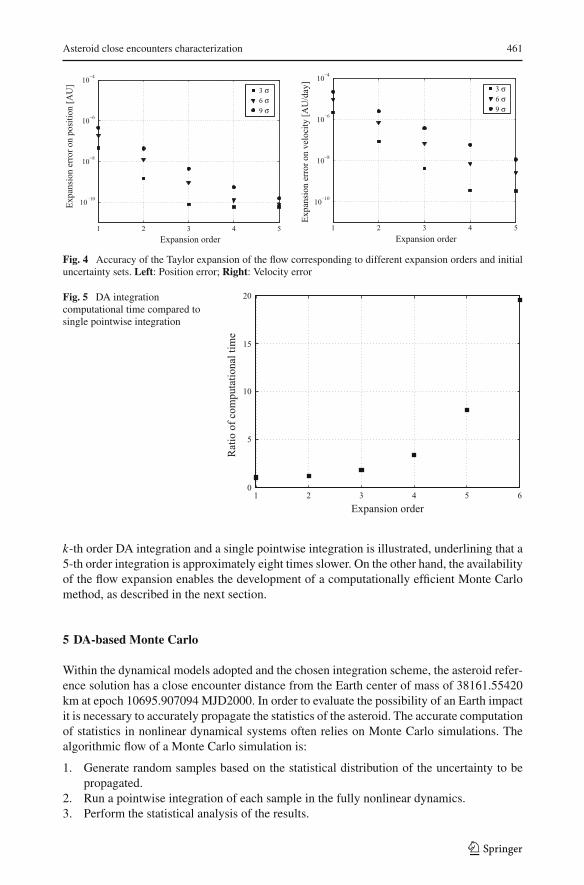
the Taylor representation of the flow at the corners of the initial set, with respect to the point-wise integration of the same points. Initial widths of 3, 6, and 9 σ and expansion orders from 1to 5 are considered. The expansion error decreases when higher expansion orders are selectedand when smaller uncertain sets are considered. The errors tend to decrease exponentiallywith the expansion order, until reaching a lower limit of approximately 5 × 10−11 [AU] onposition and 3 × 10−10 [AU/day] on velocity. It is worth noticing that a fifth order expansionguarantees a gain of approximately three order of magnitude in the flow representation withrespect to linear methods. This gain can be crucial when impact probability and/or resonantreturns are studied. The figure clearly shows that Taylor polynomial accuracy is a function ofboth the expansion order and domain width. The drawback for obtaining the Taylor expansionof the flow with respect to the initial condition is the computational time to perform a singleintegration, as shown in Fig. 5. In this figure the ratio between the computational time of a

123


Fig. 4 Accuracy of the Taylor expansion of the flow corresponding to different expansion orders and initialuncertainty sets. Left: Position error; Right: Velocity error

Fig. 5 DA integrationcomputational time compared tosingle pointwise integration

k-th order DA integration and a single pointwise integration is illustrated, underlining that a5-th order integration is approximately eight times slower. On the other hand, the availabilityof the flow expansion enables the development of a computationally efficient Monte Carlomethod, as described in the next section.

5 DA-based Monte Carlo

Within the dynamical models adopted and the chosen integration scheme, the asteroid refer-ence solution has a close encounter distance from the Earth center of mass of 38161.55420km at epoch 10695.907094 MJD2000. In order to evaluate the possibility of an Earth impactit is necessary to accurately propagate the statistics of the asteroid. The accurate computationof statistics in nonlinear dynamical systems often relies on Monte Carlo simulations. Thealgorithmic flow of a Monte Carlo simulation is:

1. Generate random samples based on the statistical distribution of the uncertainty to bepropagated.

2. Run a pointwise integration of each sample in the fully nonlinear dynamics.3. Perform the statistical analysis of the results.

123


There are three critical disadvantages when using this approach:

– convergence of the statistics usually requires a large number of sample trajectories to bepropagated,

– the simulation needs to be repeated for different initial distributions,– it does not provide the user with analytical information, useful for additional analyses.

These problems affect both the computational burden associated to the Monte Carlo sim-ulation and its validity for different statistics (Park and Scheeres 2006). The previous draw-backs become dramatic when thousands of long-term integrations are required, as for theanalysis of possible NEO close encounter with the Earth (Milani et al. 2002).

In Sect. 3 it has been shown that a single DA integration delivers an arbitrary order Taylorexpansion of the flow of the ODE, which is analytic. Furthermore, it has been remarked thatthe accuracy of the map expansion can be controlled by acting on the expansion order. Forthese reasons, it is possible to substitute the thousands of pointwise integrations requiredfor classical Monte Carlo simulations with an equal number of map evaluations, i.e. fastpolynomials evaluations.

The resulting DA-based Monte Carlo simulation can be summarized as:

1. Perform a single DA integration selecting the expansion order according to the demandedaccuracy.

2. Generate random samples based on the statistical distribution of the uncertainty to bepropagated.

3. Evaluate the flow expansion map for all the samples, requiring only fast polynomialevaluations.

4. Perform the statistical analysis of the results.

The ratio between the computational time of a DA-based Monte Carlo simulation and itspointwise counterpart is given by

tn + nstens t0

, (21)

where tn , te, and t0 are the computational times of a k-th order DA integration, a flow mapevaluation, and a pointwise integration, respectively; and ns is the number of samples of theMonte Carlo simulation. The computational cost of a Taylor map evaluation depends on theexpansion order, but it is negligible compared to a pointwise integration. For this reason,expression (21) can be approximated by m

ns, in which m is the ratio between the computa-

tional time of a k-th order DA integration and a pointwise integration (see Fig. 5). The valueof m strongly depends on the expansion order, but it is few orders of magnitude smaller thanthe number of samples required for a good representation of the statistics. For this reason,the ratio m

nsis small, proving that the proposed DA-based Monte Carlo simulation is com-

putationally efficient. As an example, in Sect. 6.3, Fig. 11 will show that the computationaltime is reduced by a factor of at least 100 for 10000 virtual asteroids.

In case new statistics need to be propagated, it is not necessary to perform an additionalDA integration as only steps 2–4 are required. Furthermore, if the statistical analysis is per-formed for a different final time, the possibility of obtaining Taylor expansions with respectto the final time can be exploited (see Sect. 6.1). Moreover, as the flow expansion is analyti-cal, an analytic framework is delivered. In conclusion, all the major drawbacks of a classicalMonte Carlo approach are circumvented. These properties are better highlighted in Sect. 6by applying the algorithm to the study of Apophis’ close encounter with the Earth in 2029.

123


6 Apophis close encounter study

As highlighted by Milani et al. (2000), impact solutions could occur for different virtual aster-oids at a time when the nominal asteroid is far from the Earth. For this reason, performingDA-based Monte Carlo simulations using the Taylor expansion of the flow at the epoch ofthe CED of the nominal solution is not appropriate, as each virtual asteroid belonging to theset of possible initial conditions has a different close encounter epoch.

A DA-based algorithm is introduced to reduce the computation of the CED, as well as itsassociated epoch, to the simple evaluation of polynomials for each virtual asteroid. Beingat the basis of the algorithm, a technique is illustrated in Sect. 6.1 to obtain the arbitraryorder Taylor expansion of the flow of ODE also with respect to the final time. The algorithmfor the computation of the Taylor expansion of the CED is then presented and applied toApophis’ case. The results obtained by running on it the DA-based Monte Carlo algorithmare illustrated.

6.1 High order expansion of the flow in time

The algorithm for the computation of the CED relies on the availability of the Taylor expan-sion of the flow of the ODE with respect to both the initial condition and the final integrationtime. In Sect. 3 it was shown how the flow expansion with respect to the initial condition canbe computed; in the following we explain how the expansion in the final time is achieved.

Consider the ODE system

dxdt

= f (x, t) (22)

to be integrated from t = t0 to t = t f . Suppose the Taylor expansion of the flow with respectto t f is of interest. We first shift the starting time by introducing the variable

t = t − t0. (23)

Using the variable t , equation (22) reads

dxdt

= f (x, t + t0), (24)

and it must be integrated from t = 0 to t = t f − t0. Then, we introduce the variable

τ = tt f − t0

. (25)

Consequently,

dt = (t f − t0) dτ (26)

and equation (24) now reads

dxdτ

= (t f − t0) · f (x, t0 + (t f − t0)τ ), (27)

that must be integrated from τ = 0 to τ = 1. Integrating Eq. 27 from τ = 0 to τ = 1is equivalent to integrate the original ODE (22) from t = t0 to t = t f . However, a majoradvantage can be highlighted: the final time t f , as well as the initial time t0, have been movedfrom the integration interval to the ODE right hand side, where they appear as parameters.

123


Fig. 6 Apophis’ distance fromthe Earth: comparison betweenthe pointwise integration and theTaylor expansion of the flow withrespect to the final integrationepoch

This allows the flow of the ODE to be expanded also with respect to the final epoch. Morespecifically, the final time t f can be initialized as a DA variable:

[t f ] = t f + δt f , (28)

in which t f is the reference final epoch. Then, Eq. 27 is integrated from τ = 0 to τ = 1.Carrying out all the algebraic operations involved in the integration scheme in the DA frame-work allows the dependence of the solution on δt f to be carried forward all throughout theintegration. The result at time τ = 1 is

[x f ] = x f + Mx f (δt f ); (29)

i.e., the Taylor expansion of the final solution with respect to the final time. Note that theTaylor expansion of the solution with respect to the initial condition and the final time canbe obtained by initializing both x0 and t f as DA variables.

The previous technique can be immediately applied to the integration of Apophis’ motionin order to obtain the Taylor expansion of the final position and velocity with respect tothe final epoch. In order to show the performances of the algorithm, set the initial condi-tion x0 to be the nominal Apophis’position and velocity at the initial epoch t0, and choosethe reference epoch t f to be the epoch of the close encounter for the nominal Apophis’initial condition. The DA-based RKF78 scheme is then used to expand the solution of theODE governing the asteroid motion with respect to t f . Figure 6 compares the nominal Apo-phis’ distance from the Earth obtained through a pointwise integration with that computedby evaluating the Taylor expansion of Apophis’ position with respect to t f , in the inter-val t f − 0.05 days < t f < t f + 0.05 days. More specifically, the results corresponding tothree different expansion orders are illustrated. As it can be seen, the accuracy of the Taylorrepresentation increases with the expansion order.

The accuracy of the Taylor representations is better assessed in Fig. 7. In particular, theabsolute difference between the results of the pointwise integration and Taylor expansionevaluation is plotted. As expected, the error is maximum at the boundary of the interval,whereas it decreases toward the center; i.e., toward the reference epoch of the Taylor expan-sions. The fifth order expansion in time guarantees an accuracy comparable with that in thetransversal coordinates for a time interval consistent with the analysis proposed in Sect. 6.3.

123


Fig. 7 Analysis of the error ofthe Taylor expansion of the flowwith respect to the finalintegration epoch for Apophis’position

−0.05 0 0.05

10−10

10−5

δ tf [day]

Exp

ansi

on e

rror

[AU

]1st order3rd order5th order

The accuracy analyses presented in this section and in Sect. 4.2 are based on checkinghow well the coordinates are predicted by the flow map versus direct integration. It is worthmentioning that in principle it is possible to get rigorous error bounds on the maps by usingTaylor models (TM) and Taylor model integrators (Hoefkens et al. 2003). As the outcomeof a TM integration is the validated enclosure of the flow of the dynamics, a single integra-tion (without any further additional analysis) would suffice for the study of Apophis’ closeencounter. On the other hand, the use of TM requires a careful coding of both the dynamicalmodel and the ephemeris function in order to efficiently compute the rigorous enclosure of theflow during the asteroid’s close encounter phase. This aspect is currently under investigationby the authors.

6.2 CED algorithm

Let us suppose the close approach of the nominal asteroid occurs at the epoch t f , and considerthe integration of the asteroid dynamics in the form (27) from t = t0 to t = t f . Initialize theinitial state and the final integration epoch as DA variables; i.e.,

[x0] = x0 + δx0[t f

]= t f + δt f ,

(30)

where x0 is the initial condition corresponding to the nominal asteroid. Using the DA-basedRKF78 integrator and the technique introduced in Sect. 6.1 obtain the map

[x f ] = x f + Mx f (δx0, δt f ). (31)

The map (31) is the k-th order Taylor expansion of the flow of (27) with respect to the initialcondition and the final epoch about their nominal values x0 and t f . Based on a mere DA-based computation, the final solution x f can be used to compute the Taylor expansion ofdistance from the Earth

[d f ] = d f + Md f (δx0, δt f ). (32)

More specifically, map (32) describes how the distance varies depending on the virtual aster-oid and the final integration epoch.

123


Using the derivation operator available in the DA framework, the Taylor expansion of thederivative d ′

f = d(d f )/dt f can be obtained

[d ′f ] = d ′

f + Md ′f(δx0, δt f ). (33)

The constant part of the map (33), d ′f , is the derivative of the distance from the Earth of the

nominal solution at its close encounter; i.e., at CED epoch. Consequently, this is a stationarypoint for the nominal solution, and d ′

f = 0. Then, the map (33) reduces to

δd ′f = Md ′

f(δx0, δt f ), (34)

in which we omit the bracket operator for the sake of a simpler notation. Consider the map(

δd ′f

δx0

)=

(Md ′

f

Ix0

) (δx0δt f

), (35)

which is built by concatenating Md ′f

with the identity map for δx0. Map (35) can now beinverted to obtain

(δx0δt f

)=

(Md ′

f

Ix0

)−1 (δd ′

fδx0

). (36)

This is a full nonlinear map inversion that is obtained by applying the algorithm illustratedin Berz (1999b). This algorithm reduces the map inversion problem to the solution of anequivalent fixed point problem, which can be solved with a fixed amount of effort in the DAsetting.

Map (32) is then concatenated to the identity map for δt f to obtain(

d fδt f

)=

(Md f

It f

) (δx0δt f

). (37)

Map (37) can now be composed with map (36) to obtain

(d fδt f

)=

(Md f

It f

)◦

(Md ′

f

Ix0

)−1 (δd ′

fδx0

), (38)

which relates d f and δt f to the displacements of the derivative of the final distance δd ′f and

of the initial state vector of the virtual asteroid δx0 from their values. As for the referencevalue d ′

f = 0, the necessary condition for CED computation is

δd ′f = 0. (39)

Substituting into (38) yields

(d f

∗

δt f∗

)=

(Md f

It f

)◦

(Md ′

f

Ix0

)−1 (0

δx0

). (40)

Eventually, map (40) delivers the desired explicit relation between the CED (d f∗) and the

epoch at which it is reached (t f +δt f∗) with the displacement δx0 in terms of Taylor polyno-

mials. Given any virtual asteroid belonging to the initial set (which corresponds to a specificvalue of the displacement δx0), the simple evaluation of the polynomials in (40) delivers theCED and the epoch at which it is reached. In this way, the problem highlighted by Milani etal. (2000) is solved.

123


6.3 CED statistical analysis

The DA-based Monte Carlo simulation introduced in Sec. 5 is run on map (40) to perform thenonlinear mapping of the initial uncertainties on the close encounter distance (CED). Morespecifically, 10000 virtual asteroids are generated with a normal random distribution withmean value and standard deviation as in Table 1. For each sample, the displacement withrespect to the nominal initial conditions is computed and map (40) is evaluated to obtain itsCED and the associated epoch. The result is reported in Fig. 8(left) in terms of probabilitydistribution for the CED. The analysis of the results shows that the mean value is 38161.54km with a standard deviation of 492.1 km, thus the possibility of having an Earth impact in2029 is ruled out.

For the same virtual asteroids, map (40) is also evaluated to obtain the close encounterepochs. The result is presented in Fig. 8(right) in terms of the probability distribution of thedisplacement δt f

∗ from the nominal epoch t f . The maximum displacement is of the order of30 s, which is compatible with the accuracy of the Taylor expansion with respect to the finalepoch shown in Fig. 7. In Fig. 9 the 10000 virtual asteroids are plotted in the CED-δt∗f plane.

Fig. 8 Monte Carlo analysis of virtual asteroids close encounter distances (CED). Left: The distances; Right:The epochs

Fig. 9 CED vs δt∗f for 10000virtual asteroids

123


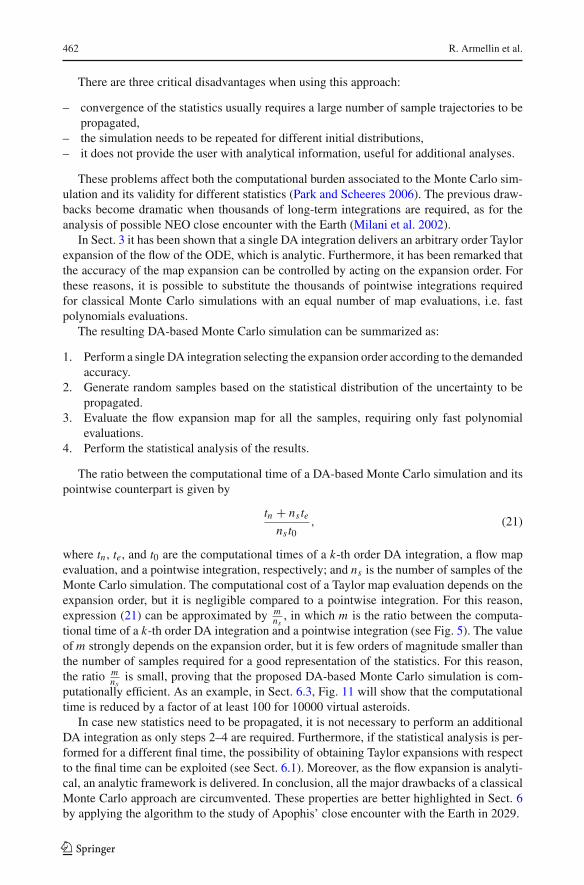
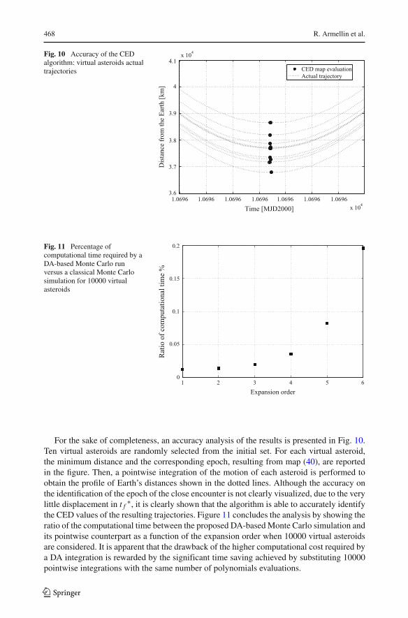
Fig. 10 Accuracy of the CEDalgorithm: virtual asteroids actualtrajectories

Fig. 11 Percentage ofcomputational time required by aDA-based Monte Carlo runversus a classical Monte Carlosimulation for 10000 virtualasteroids

For the sake of completeness, an accuracy analysis of the results is presented in Fig. 10.Ten virtual asteroids are randomly selected from the initial set. For each virtual asteroid,the minimum distance and the corresponding epoch, resulting from map (40), are reportedin the figure. Then, a pointwise integration of the motion of each asteroid is performed toobtain the profile of Earth’s distances shown in the dotted lines. Although the accuracy onthe identification of the epoch of the close encounter is not clearly visualized, due to the verylittle displacement in t f

∗, it is clearly shown that the algorithm is able to accurately identifythe CED values of the resulting trajectories. Figure 11 concludes the analysis by showing theratio of the computational time between the proposed DA-based Monte Carlo simulation andits pointwise counterpart as a function of the expansion order when 10000 virtual asteroidsare considered. It is apparent that the drawback of the higher computational cost required bya DA integration is rewarded by the significant time saving achieved by substituting 10000pointwise integrations with the same number of polynomials evaluations.

123


7 Conclusions

The paper introduced a Monte Carlo simulation based on the high order Taylor expansion ofthe flow of ODE, enabled by the use of differential algebra. Being based on the replacementof pointwise integrations with fast evaluation of polynomials, the proposed algorithm guar-antees significant computational time savings. The accuracy of the algorithm can be suitablytuned by varying the flow expansion order. Furthermore, the availability of analytic Taylorexpansions and the use of DA embedded tools as map inversion, composition, and deriva-tion allow the user to compute arbitrary order maps of the quantities on which the statisticalanalysis is performed; thus, the algorithm is not limited to the flow of ODE. More specifically,a technique for the automatic computation of both CED and CED epochs for all the virtualasteroids belonging to the initial uncertainty cloud has been developed. The efficiency andeffectiveness of the methods are proven by applying them to the analysis of Apophis’ closeencounter with the Earth occurring in April 2029. In particular, it is shown that

– the nonlinear mapping of uncertainties can be performed for any complex and arbitrarydynamics, even when long-term integrations are required;

– a fifth order expansion increases the accuracy of the computation of the CED by approx-imately two orders of magnitude with respect to classical linear methods;

– the expansion in time allows for the proper identification of the CED epoch for all thevirtual asteroids.

As an additional result, the occurrence of an impact with the Earth in April 2029 can be ruledout.

Acknowledgments This work was inspired by Park and Scheeres (2006) and was partially conducted underthe ESA Ariadna study “NEO Encounter 2029”. The authors are grateful to Dario Izzo for having encouragedthe work and to Jon Giorgini for his precious comments.

References

Battin, R.H.: An Introduction to the Mathematics and Methods of Astrodynamics. AIAA EducationSeries, New York (1968)

Berges, J., Rousseau, S., Perot E.: A Numerical Predictor-Corrector Guidance Algorithm for the Mars SampleReturn Aerocapture. AAAF, 14–66, March (2001)

Bernelli-Zazzera, F., Berz, M., Lavagna, M., Makino, K., Armellin, R., Di Lizia, P., Jagasia, R., Topputo,F.: NEO Encounter 2029: Orbital Prediction via Differential Algebra and Taylor Models. Final Report,Ariadna id: 08-4303, Contract No. 20271/06/NL/HI (2009)

Berz, M.: The new method of TPSA algebra for the description of beam dynamics to high orders. TechnicalReport AT-6:ATN-86-16, Los Alamos National Laboratory (1986)

Berz, M.: The method of power series tracking for the mathematical description of beam dynamics. NuclearInstrum. Meth. A258, 431 (1987)

Berz, M.: High-order computation and normal form analysis of repetitive systems. Phys. Particle Accel. AIP249, 456 (1991)

Berz, M., Joh, K., Nolen, J.A., Sherrill, B.M., Zeller, A.F.: Reconstructive correction of aberration in nuclearparticle spectrographs. Phys. Rev. C 47, 537–544 (1993)

Berz, M.: Differential Algebraic Techniques. Entry in Handbook of Accelerator Physics and Engineer-ing. World Scientific, New York (1999a)

Berz, M.: Modern Map Methods in Particle Beam Physics. Academic Press, London (1999b)Berz M., Makino K.: COSY INFINITY version 9 reference manual. MSU Report MSUHEP-060803, Michigan

State University, East Lansing, MI 48824, pp. 1–84 (2006)Chesley, S.R., Milani, A.: An automatic earth-asteroid collision monitoring system. Bull. Am. Astron.

Soc. 32, 682 (2000)

123


Chodas, P.W., Yeomans, D.K.: Predicting close approaches and estimating impact probabilities for near-Earthprojects. AAS/AIAA Astrodynamics Specialists Conference, Girdwood, Alaska (1999)

Crassidis, J.L., Junkins, J.L.: Optimal Estimation of Dynamics Systems. pp. 243–410. CRC Press LLC, BocaRaton, FL (2004)

Di Lizia, P., Armellin, R., Lavagna, M.: Application of high order expansions of two-point boundary valueproblems to astrodynamics. Celest. Mech. Dyn. Astron. 102, 355–375 (2008)

Erdelyi, B., Bandura, L., Nolen, J., Manikonda, S.: Code development for next-generation high-intensity largeacceptance fragment separators. In: Proceedings of PAC07, Albuquerque, New Mexico, USA (2007)

Giorgini, J.D., Benner, L.A.M., Ostro, S.J., Nolan, M.C., Busch, M.W.: Predicting the earth encounters of(99942) apophis. Icarus 193, 1–19 (2008)

Griffith, T.D., Turner, J.D., Vadali, S.R., Junkins, J.L.: Higher order sensitivities for solving nonlineartwo-point boundary-value problems. In: AIAA/AAS Astrodynamics Specialist Conference and Exhibit,Providence, Rhode Island, August 16–19 (2004)

Hoefkens, J., Berz, M., Makino, K.: Controlling the wrapping effect in the solution of ODEs for asteroids.Reliable Comput. 8, 21–41 (2003)

Junkins, J., Akella, M., Alfriend, K.: Non-Gaussian error propagation in orbit mechanics. J. Astronaut.Sci. 44, 541–563 (1996)

Junkins, J., Singla, P.: How nonlinear is it? A tutorial on nonlinearity of orbit and attitude dynamics. J. Astro-naut. Sci. 52, 7–60 (2004)

Maybeck, P.S.: Stochastic Models, Estimation, and Control. pp. 159–271. Academic Press, New York (1982)Milani, A., Chesley, S.R., Valsecchi, G.B.: Asteroid close encounters with Earth: Risk assessment. Planet.

Space Sci. 48, 945–954 (2000)Milani, A., Chesley, S.R., Chodas, P.W., Valsecchi, G.B.: Asteroid close approaches: analysis and potential

impact detection. Asteroids III, pp. 89–101 (2002)Montenbruck, O., Gill, E.: Satellite Orbits. pp. 257–291. 2nd edn. Springer, New York (2001)Park, R., Scheeres, D.: Nonlinear mapping of Gaussian statistics: theory and applications to spacecraft trajec-

tory design. J. Guidance Control Dyn. 29, 1367–1375 (2006)Park, R.S., Scheeres, D.J.: Nonlinear semi-analytic methods for trajectory estimation. J. Guidance Control

Dyn. 30, 1668–1676 (2007)Seidelmann, P.K.: Explanatory Supplement to the Astronomical Almanac. University Science Books, Mill

Valley, California (1992)Vokrouhlický, D., Chesley, S.R., Milani, A.: On the observability of radiation forces acting on near-earth a

steroids. Celest. Mech. Dyn. Astron. 81, 149–165 (2001)

123

asteroid close encounters characterization using differential algebra

Documents