Automata Learningand its ApplicationsA thesis submitted in full�lement of the requirementsfor the degree of Doctor of PhilosophyDana Ron

Submitted to the Senate of the Hebrew University in the year 1995

This work was carried outunder the supervision of Dr. Naftali Tishby

AcknowledgmentsFirst of all I would like to thank my advisor, Tali Tishby who introduced me to the area of MachineLearning. I learned a great deal from Tali, but what I think makes him especially exceptionalas an advisor, is that he not only taught me much, but also encouraged me to build up my ownpersonal opinions and views about research in learning theory. I also owe Tali for being extremelysupportive all along the way, from the �rst summer in which he persuaded me to go to COLTand to visit Bell Labs, and until this present day.I would like to thank Ronitt Rubinfeld who is both a great colleague and a dear friend. Imade my �rst steps in learning theory research with Ronitt who didn't allow me to give up whenit seemed there was no progress, and continued encouraging me throughout the years.I would next like to thank Mike Kearns and Rob Schapire whom I view metaphorically as myresearch \uncles". I had some of my happiest and most exciting times while working with themin Bell Labs (not to mention some of the best sushi and saki..)I owe much to Yoram Singer with whom I did a substantial part of the work presented here.Through our collaboration I not only learned a lot about practical problems in Machine Learning,but I also regained faith in the possibility of truly combining theoretical and practical research.I enjoyed very much working with Yoav Freund, and am especially glad that we managed toovercome the periods in which we su�ered from lack of faith. I gained much from working withYishay Mansour who never ceases to impress me with his broad knowledge. I would like to thankIlan Kremer and Noam Nisan who got me interested in working on problems in CommunicationComplexity which was a stimulating change. I enjoyed collaborating with Andrew Ng who is bothan excellent programmer as well as a talented theoretician. I had great fun working with MichalParnas, (despite all her teasing), and perhaps \our robots" can once come back to life. I enjoyedworking with Linda Sellie who is a great contributor of original ideas.Special thanks to Sha� Goldwasser for calming me down so many times during our drives toJerusalem and in general for serving as a role model for me.I am very grateful to Michael Ben-Or, Nati Linial, Eli Shamir and Avi Wigderson who werealways happy to answer questions and give advice. In general, I believe that my choice to returnto the Hebrew University for my PhD was one of the best decisions I made.I would like to thank all members of my family who had in uence on various importanti

iidecisions I made in life. To my brother, David, who persuaded me not to study Medicine. Tomy mother, Arza, who came up with the idea that I study Computer Science, and to my father,Amiram, who thought that I should also study a real science, i.e., Physics. And lastly to mysister, Ruthie, who never told me what to do.Thanks to the Eshkol Fellowship for its support during the last two years, which allowed meto put almost all my e�orts into research. Also thanks to AT&T Bell Laboratories which hostedme for two summers and where part of the work presented in this thesis was done.Finally, I have reached the hardest part in which I would like to thank my beloved Oded.Hard, because no sequence of words can faithfully explain all that Oded has given me duringthese last few years and which is partly realized in this work. Perhaps the following song (fromKorin Al'al's Forbidden Fruit), can capture a little of what I would like to say:mini c`n daxd xakmind ipt lr mibiltn epgp`segd on epwgx xakmiiny ieevwn enkzezixa c`n daxd xakgexd mr epzxk ik epinicef len df epxzeperexw yxtn mrdlek dxiqdykegexd on zcrxpzerncd on ,dtaegeln ,mid inejl zxne` ip`ici izya ahid feg`iige jiig seg `id efd dxiqd

ContentsAbstract 11 Introduction 31.1 The PAC Model and Some of its Extensions : : : : : : : : : : : : : : : : : : : : : : 51.2 Background on Automata Learning : : : : : : : : : : : : : : : : : : : : : : : : : : : 81.2.1 Learning Deterministic Automata : : : : : : : : : : : : : : : : : : : : : : : 81.2.2 Learning Probabilistic Automata : : : : : : : : : : : : : : : : : : : : : : : : 111.3 Overview of Results Presented in this Thesis : : : : : : : : : : : : : : : : : : : : : 121.3.1 Results on DFA Learning : : : : : : : : : : : : : : : : : : : : : : : : : : : : 131.3.2 Results on PFA Learning : : : : : : : : : : : : : : : : : : : : : : : : : : : : 141.4 Suggestions for Further Research : : : : : : : : : : : : : : : : : : : : : : : : : : : : 151.5 Other Results Which Were Not Included in This Thesis : : : : : : : : : : : : : : : 172 Preliminaries 232.1 Strings and Sets of Strings : : : : : : : : : : : : : : : : : : : : : : : : : : : : : : : : 232.2 Deterministic Finite Automata : : : : : : : : : : : : : : : : : : : : : : : : : : : : : 242.3 Probabilistic Finite Automata : : : : : : : : : : : : : : : : : : : : : : : : : : : : : : 242.4 Learning Deterministic Automata : : : : : : : : : : : : : : : : : : : : : : : : : : : : 252.4.1 PAC Learning: with/without Membership Queries : : : : : : : : : : : : : : 262.4.2 Exact Learning: with/without Reset : : : : : : : : : : : : : : : : : : : : : : 262.4.3 Bounded Mistake Online Learning: with/without Reset : : : : : : : : : : : 272.4.4 Noise Models : : : : : : : : : : : : : : : : : : : : : : : : : : : : : : : : : : : 282.5 Learning Probabilistic Automata : : : : : : : : : : : : : : : : : : : : : : : : : : : : 282.6 Some Useful Inequalities : : : : : : : : : : : : : : : : : : : : : : : : : : : : : : : : : 29iii

iv CONTENTSI Deterministic Automata 313 Learning Typical Automata from Random Walks 333.1 Introduction : : : : : : : : : : : : : : : : : : : : : : : : : : : : : : : : : : : : : : : : 333.2 Preliminaries : : : : : : : : : : : : : : : : : : : : : : : : : : : : : : : : : : : : : : : 353.3 Learning With a Reset : : : : : : : : : : : : : : : : : : : : : : : : : : : : : : : : : : 373.3.1 Combinatorics : : : : : : : : : : : : : : : : : : : : : : : : : : : : : : : : : : 373.3.2 The Algorithm : : : : : : : : : : : : : : : : : : : : : : : : : : : : : : : : : : 383.4 Learning Without a Reset : : : : : : : : : : : : : : : : : : : : : : : : : : : : : : : : 413.4.1 Combinatorics : : : : : : : : : : : : : : : : : : : : : : : : : : : : : : : : : : 423.4.2 The Algorithm : : : : : : : : : : : : : : : : : : : : : : : : : : : : : : : : : : 443.5 Replacing Randomness with Semi-Randomness : : : : : : : : : : : : : : : : : : : : 474 Exactly Learning Automata with Small Cover Time 494.1 Introduction : : : : : : : : : : : : : : : : : : : : : : : : : : : : : : : : : : : : : : : : 494.2 Exact Learning with a Reset : : : : : : : : : : : : : : : : : : : : : : : : : : : : : : 514.3 Exact Learning without a Reset : : : : : : : : : : : : : : : : : : : : : : : : : : : : : 544.4 Exact Learning in the Presence of Noise : : : : : : : : : : : : : : : : : : : : : : : : 58II Probabilistic Automata 635 Learning Prob. Automata with Variable Memory 655.1 Introduction : : : : : : : : : : : : : : : : : : : : : : : : : : : : : : : : : : : : : : : : 655.2 Preliminaries : : : : : : : : : : : : : : : : : : : : : : : : : : : : : : : : : : : : : : : 675.2.1 Probabilistic Su�x Automata : : : : : : : : : : : : : : : : : : : : : : : : : : 675.2.2 Prediction Su�x Trees : : : : : : : : : : : : : : : : : : : : : : : : : : : : : : 695.2.3 The Learning Model : : : : : : : : : : : : : : : : : : : : : : : : : : : : : : : 705.3 Emulation of PSA's by PST's : : : : : : : : : : : : : : : : : : : : : : : : : : : : : : 725.4 The Learning Algorithm : : : : : : : : : : : : : : : : : : : : : : : : : : : : : : : : : 735.5 Analysis of the Learning Algorithm : : : : : : : : : : : : : : : : : : : : : : : : : : : 755.6 Applications : : : : : : : : : : : : : : : : : : : : : : : : : : : : : : : : : : : : : : : : 795.6.1 Correcting Corrupted Text : : : : : : : : : : : : : : : : : : : : : : : : : : : 795.6.2 Building A Simple Model for E.coli DNA : : : : : : : : : : : : : : : : : : : 82

CONTENTS v6 Learning Acyclic Probabilistic Automata 856.1 Introduction : : : : : : : : : : : : : : : : : : : : : : : : : : : : : : : : : : : : : : : : 856.2 Preliminaries : : : : : : : : : : : : : : : : : : : : : : : : : : : : : : : : : : : : : : : 876.2.1 The Learning Model : : : : : : : : : : : : : : : : : : : : : : : : : : : : : : : 886.3 On the Intractability of Learning PFA's : : : : : : : : : : : : : : : : : : : : : : : : 896.4 The Learning Algorithm : : : : : : : : : : : : : : : : : : : : : : : : : : : : : : : : : 916.5 Correctness of the Learning Algorithm : : : : : : : : : : : : : : : : : : : : : : : : : 956.6 Applications : : : : : : : : : : : : : : : : : : : : : : : : : : : : : : : : : : : : : : : : 956.6.1 Building Stochastic Models for Cursive Handwriting : : : : : : : : : : : : : 966.6.2 Building Pronunciation Models for Spoken Words : : : : : : : : : : : : : : : 98Bibliography 100A Supplements for Chapter 3 113A.1 Proof of Theorem 3.2 : : : : : : : : : : : : : : : : : : : : : : : : : : : : : : : : : : : 113A.2 Learning Typical Automata in the PAC Model : : : : : : : : : : : : : : : : : : : : 116B Supplements for Chapter 4 119C Supplements for Chapter 5 121C.1 Proof of Theorem 5.1 : : : : : : : : : : : : : : : : : : : : : : : : : : : : : : : : : : : 121C.2 Emulation of PST's by PFA's : : : : : : : : : : : : : : : : : : : : : : : : : : : : : : 123C.3 Proofs of Technical Lemmas and Theorems : : : : : : : : : : : : : : : : : : : : : : 124D Supplements for Chapter 6 131D.1 Analysis of the Learning Algorithm : : : : : : : : : : : : : : : : : : : : : : : : : : : 131D.1.1 A Good Sample : : : : : : : : : : : : : : : : : : : : : : : : : : : : : : : : : : 132D.1.2 Proof of Theorem 6.2 : : : : : : : : : : : : : : : : : : : : : : : : : : : : : : 135D.2 An Online Version of the Algorithm : : : : : : : : : : : : : : : : : : : : : : : : : : 138D.2.1 An Online Learning Model : : : : : : : : : : : : : : : : : : : : : : : : : : : 139D.2.2 An Online Learning Algorithm : : : : : : : : : : : : : : : : : : : : : : : : : 139

vi CONTENTS

List of Figures3.1 Pseudocode for algorithm Reset. : : : : : : : : : : : : : : : : : : : : : : : : : : : : 394.1 Algorithm Exact-Learn-with-reset : : : : : : : : : : : : : : : : : : : : : : : : : 524.2 AlgorithmExact-Learn-Given-Homing-Sequence and AlgorithmExact-Learn554.3 Algorithm Exact-Noisy-Learn : : : : : : : : : : : : : : : : : : : : : : : : : : : : 584.4 Procedure Execute-Homing-Sequence : : : : : : : : : : : : : : : : : : : : : : : 595.1 Left: A 2-PSA. The strings labeling the states are the su�xes corresponding tothem. Bold edges denote transitions with the symbol `1', and dashed edges denotetransitions with `0'. The transition probabilities are depicted on the edges. Middle:A 2-PSA whose states are labeled by all strings in f0; 1g2. The strings labeling thestates are the last two observed symbols before the state was reached, and henceit can be viewed as a representation of a Markov chain of order 2. It is equivalentto the (smaller) 2-PSA on the left. Right: A prediction su�x tree. The predictionprobabilities of the symbols `0' and `1', respectively, are depicted beside the nodes,in parentheses. : : : : : : : : : : : : : : : : : : : : : : : : : : : : : : : : : : : : : : 705.2 Algorithm Learn-PSA : : : : : : : : : : : : : : : : : : : : : : : : : : : : : : : : : 745.3 An illustrative run of the learning algorithm. The prediction su�x trees createdalong the run of the algorithm are depicted from left to right and top to bottom.At each stage of the run, the nodes from �T are plotted in dark grey while the nodesfrom �S are plotted in light grey. The alphabet is binary and the predictions of thenext bit are depicted in parenthesis beside each node. The �nal tree is plotted onthe bottom right part and was built in the second phase by adding all the missingsons of the tree built at the �rst phase (bottom left). Note that the node labeledby 100 was added to the �nal tree but is not part of any of the intermediate trees.This can happen when the probability of the string 100 is small. : : : : : : : : : : 765.4 Correcting corrupted text. : : : : : : : : : : : : : : : : : : : : : : : : : : : : : : : : 81vii

viii LIST OF FIGURES5.5 The di�erence between the log-likelihood induced by a PSA trained on data takenfrom intergenic regions and a PSA trained on data taken from coding regions. Thetest data was taken from intergenic regions. In 90% of the cases the likelihood ofthe �rst PSA was higher. : : : : : : : : : : : : : : : : : : : : : : : : : : : : : : : : 836.1 Algorithm Learn-APFA : : : : : : : : : : : : : : : : : : : : : : : : : : : : : : : : 926.2 Function Similar : : : : : : : : : : : : : : : : : : : : : : : : : : : : : : : : : : : : : 926.3 Procedure Fold : : : : : : : : : : : : : : : : : : : : : : : : : : : : : : : : : : : : : : 936.4 Procedure AddSlack : : : : : : : : : : : : : : : : : : : : : : : : : : : : : : : : : : 936.5 Procedure GraphToPFA : : : : : : : : : : : : : : : : : : : : : : : : : : : : : : : : 936.6 An illustration of the folding operation. The graph on the right is constructed fromthe graph on the left by merging the nodes v1 and v2. The di�erent edges representdi�erent output symbols: gray is 0, black is 1 and bold black edge is �. : : : : : : : 946.7 Synthetic cursive letters, created by random walks on the 26 APFA's. : : : : : : : 966.8 Temporal segmentation of the word impossible. The segmentation is performedby evaluating the probabilities of the APFA's which correspond to the letter con-stituents of the word. : : : : : : : : : : : : : : : : : : : : : : : : : : : : : : : : : : : 976.9 An example of pronunciation models based on APFA's for the words have, hadand often trained from the TIMIT database. : : : : : : : : : : : : : : : : : : : : : 99B.1 Automata M1 and M2 described in the Appendix : : : : : : : : : : : : : : : : : : : 120D.1 Left: Part of the original automaton, M , that corresponds to the copies on theright part of the �gure. Right: The di�erent types of copies of M 's states: copiesof a state are of two types major and minor. A subset of the major copies of everystate is chosen to be dominant (dark-gray nodes). The major copies of a state inthe next level are the next states of the dominant states in the current level. : : : 133D.2 Algorithm Online-Learn-APFA : : : : : : : : : : : : : : : : : : : : : : : : : : : 141E.1 Procedure Partition-Sample (Error-free Case) : : : : : : : : : : : : : : : : : : : : : 7E.2 Procedure Estimate-Error : : : : : : : : : : : : : : : : : : : : : : : : : : : : : : : : 10E.3 Procedure Partition-Erroneous-Sample (Initial Partition) : : : : : : : : : : : : : : 16E.4 Function Initialize-Graph : : : : : : : : : : : : : : : : : : : : : : : : : : : : : : : : 16E.5 Procedure Update-Graph : : : : : : : : : : : : : : : : : : : : : : : : : : : : : : : : 17E.6 Function Strings-Test : : : : : : : : : : : : : : : : : : : : : : : : : : : : : : : : : : 17E.7 First example target automaton. q1 is the single accepting state. : : : : : : : : : : 20

LIST OF FIGURES ixE.8 Second example target automaton. q3 is the single accepting state. : : : : : : : : : 21E.9 Procedure Label-Classes : : : : : : : : : : : : : : : : : : : : : : : : : : : : : : : : : 23E.10 Hypothesis automaton for the �rst example. : : : : : : : : : : : : : : : : : : : : : : 29E.11 Hypothesis automaton for the �rst example (minimized version). : : : : : : : : : : 29E.12 Hypothesis automaton for second example. : : : : : : : : : : : : : : : : : : : : : : 30E.13 Hypothesis automaton for second example (minimized version). : : : : : : : : : : : 31

x LIST OF FIGURES

AbstractThis thesis is a study of automata learning. Most of the work presented here is in the frame-work of Computational Learning Theory and hence emphasizes the theoretical aspects of learningalgorithms and their rigorous analysis. However, a substantial part of this work was directly mo-tivated by practical applications in human-machine interactions such as the statistical modelingof natural languages and handwriting. Thus, in addition to the formal description and analysisof learning algorithms for both deterministic and probabilistic automata, several applications ofthese algorithms are given. The thesis consists of two parts: one on learning deterministic au-tomata and one on learning probabilistic automata, where the latter are automata that generatedistributions. Since there are severe limitations on our ability to learn e�ciently both determin-istic and probabilistic automata, a common thread that passes through these two parts is thesearch for natural subclasses of automata that can be learned e�ciently.We begin the �rst part by describing e�cient algorithms for learning deterministic �niteautomata, where our approach is primarily distinguished by two features: (1) the adoption ofan average-case setting to model the \typical" labeling of a �nite automaton, while retaining aworst-case model for the underlying graph of the automaton, along with (2) a passive learningmodel in which the learner is not provided with the means to experiment with the machine,but rather must learn solely by observing the automaton's output behavior on a random inputsequence. The main contribution of this work is in presenting the �rst e�cient algorithms forlearning non-trivial classes of automata in an entirely passive learning model.We continue with an e�cient algorithm for actively learning an environment that can bedescribed by a deterministic automaton whose underlying graph has certain topological properties.The learner may perform a single walk of its choice on the automaton and observe the outputsof the states passed. It must then be able to predict correctly the output sequence correspondingto any future walk. This work was partly motivated by a game theoretical problem of playingrepeated games against a computationally bounded adversary. We also show that a variant of thisalgorithm is robust to random noise. Previous work in this model either assumed access to a verypowerful oracle, or made other limiting assumptions on the target automaton and the informationthat the learner is given.In the second part of this thesis, we give evidence to the hardness of learning general prob-abilistic automata. We show that under an assumption about the di�culty of learning parity1

2 ABSTRACTfunctions with classi�cation noise in the PAC model (a problem closely related to the longstand-ing coding theory problem of decoding a random linear code), the class of distributions de�ned byprobabilistic �nite automata is not e�ciently learnable. However, we describe e�cient algorithmsfor learning two subclasses of probabilistic automata: variable memory probabilistic automata,and acyclic state-distinguishable probabilistic automata. Research on both subclasses was directlymotivated by practical applications of modeling various natural sequences, and we present thefollowing applications of the two respective learning algorithms.We applied the algorithm for learning variable memory probabilistic automata in order toconstruct: (1) a model of the English language which we used to correct corrupted text; (2) asimple probabilistic model for E.coli DNA. We applied the algorithm for learning acyclic proba-bilistic automata in order to construct: (1) models for cursively written letters which were usedfor segmenting labeled data; (2) multiple-pronunciation models for spoken words.Moreover, the two subclasses we consider (and their respective learning algorithms) comple-ment each other. Whereas the class of variable memory probabilistic automata captures the longrange, stationary, statistical properties of the natural source, the class of acyclic probabilisticautomata captures the short sequence statistics. Together, these algorithm constitute a powerfullanguage modeling scheme. This scheme was applied to cursive handwriting recognition and maybe applicable to similar problems such as speech recognition.

Chapter 1IntroductionThe concept of learning is used in many contexts and has various interpretations. By combiningseveral dictionary de�nitions for the verb \to learn" we get: \to gain knowledge, understandingor skill by study, experience, practice, or being taught". In the context of designing machinesthat learn, learning is often interpreted as inferring rules from examples. The inferred rule isthen used to perform a related task, such as prediction or identi�cation. Learning algorithmscan be contrasted with fully determined algorithms which are designed to perform speci�c tasks,based on rules which are prede�ned by the programmer. There are many cases in which a fullydetermined algorithm or machine is the best solution to a problem. Such is the case when usinga robot to perform a well de�ned task in an assembly line, or when designing a compiler for aspeci�c programming language. However, there are other cases in which one may bene�t greatlyby employing learning in order to infer good rules from experience instead of determining themin advance, as is illustrated in the following example.Suppose that we are interested in constructing an algorithm that recognizes handwritten text.The algorithm receives as input a sequence of handwritten letters, and should output a sequenceof alphabet symbols which corresponds as well as possible to the input sequence. One approachto this problem, which we shall refer to as the fully determined approach, is to \hard-wire" a rulethat can be used to determine for every possible handwritten letter what is the alphabet symbolthat it represents. The second approach, coined the learning approach, is to design an algorithmthat tries to infer such a recognition rule from a sample of labeled data (consisting of handwrittenletters and the alphabet symbols they represent). It is important to stress that the rule inferred,though based on the sample, should perform well on new , unlabeled data, and should not only(or even necessarily) correctly label the sample data.The following two problems arise when trying to implement the fully determined approach.The �rst problem is that while a person may be able to perform the handwriting recognition taskquite easily, it is not clear what exactly is the rule he/she applies, and if it can be de�ned simplyfor the use of the algorithm. The second problem is that even if such a rule can be de�ned, it3

4 CHAPTER 1. INTRODUCTIONmay di�er greatly from writer to writer, and may be completely useless if we switch to a languagethat has a di�erent alphabet.It is clear that the learning approach does not su�er from the second problem mentioned abovesince it is adaptive in nature. Given input written by a certain writer in a certain language, it willtune itself to that writer and language and need not be tuned in advance. As for the �rst problem,by de�nition of the learning approach, the programmer is now freed from the need to preciselyde�ne an identi�cation rule. Thus, it seems that for the handwriting recognition problem andsimilar problems, the learning approach may be bene�cial.However, if we examine more carefully the brief description of the learning approach givenabove, we �nd that there are a few questions that need to be answered before we crown thisapproach as \the winner". When we say that the algorithm should infer a rule, what type of ruledo we exactly mean? Can it choose from all possible functions mapping input strings representinghandwritten letters to the output alphabet symbols? Or do we assume that the rule should bemore restricted (e.g., the rule should be a circuit of some bounded size)? If we allow the class fromwhich a rule is chosen to be very complex, then it is more likely that there exists a rule in the classthat performs well, i.e., that can label correctly a large fraction among all possible handwrittenletters. However, even if the examples were labeled exactly according to such a rule, the processof learning might become more time-consuming when the function class is more complex.Thus the goal of research in machine learning is twofold. On one hand we must try andunderstand what type of (hopefully simple) classes of rules can capture well the natural or arti�cialphenomena which are relevant to machine learning applications. On the other hand we would liketo design algorithms for learning these classes of rules. While the �nal measure of our success isthe performance of our algorithms on real data, it is important at times to separate ourselves fromreal world problems and to study the purely theoretical aspects of learning. Such studies can aidus in understanding the limits of what can be learned e�ciently by machines, as well as help usin designing algorithms that not only work well in theory, but also perform well in practice. Thelatter remains true even if the algorithms are not motivated directly by speci�c practical problems,but rather by the quest for understanding the nature and limitations of machine learning.In order to study learning theory, we must �rst have a mathematical model of learning. Themodel we use is the Probably Approximately Correct (PAC ) learning model and its extensions. ThePAC model was introduced by Valiant in his seminal paper \A Theory of the Learnable" [Val84],which initiated a �eld of research know as Computational Learning Theory . Many of the ideasused in the de�nition of this model and later in work related to this model have roots in several wellstudied areas of research, among them are Statistics, Arti�cial Intelligence, Inductive Inference,Pattern Recognition, and Information Theory. While we obviously cannot do justice here to theserich and varied areas, we suggest the following references. Vapnik's work (cf. [Vap82]) in the areaof Statistics, formalizes, addresses and answers many of the questions related to the samplecomplexity of learning algorithms. Several of Vapnik's ideas, techniques, and results were laterused in the computational learning theory literature, though he does not discuss the computationalcomplexity aspect of learning theory. Interesting discussions regarding the Arti�cial Intelligence

1.1. THE PAC MODEL AND SOME OF ITS EXTENSIONS 5view of learning can be found in [CF68, Sim83, Mic86]. Angluin and Smith [AS83] give a thoroughsurvey on Inductive Inference. The book of Duda and Hart [DH73] on Pattern Recognition, andthe book of Cover and Thomas [CT91] on Information Theory are widely used introductions tothe respective �elds.1.1 The PAC Model and Some of its ExtensionsValiant suggested a mathematical model of learning concepts from examples . A concept accordingto Valiant is a set of instances (e.g., the set of all buildings built in Israel during the late 1930's),each de�ned by a set of attributes (e.g. height of ceilings, type of balconies, location and styleof windows). Given a concept, there must exist a rule according to which instances can becategorized as belonging to the concept, or not belonging to the concept. A learning algorithm isgiven a sample of independently chosen positive and negative examples (instances which belong tothe concept, and instances which do not belong to the concept, respectively), and it must outputa rule which categorizes well new instances it has not seen in the sample. The novelty of Valiant'smodel is in the combination of the following assumptions and restrictions:� The learning algorithm has knowledge about the class of concepts , or rules, which thelearned concept belongs to. For example, if the attributes de�ning an instance are binary(e.g., is a building built of stone or not), then a rule could be some boolean function.� The probability distribution on the instances, on the other hand, is unknown, may be arbi-trary, but is �xed in the following sense. The distribution according to which the instancesin the sample are chosen is the same as the distribution by which new instances, which thealgorithm must categorize, are chosen. The assumption that the distribution is arbitrarymight make the learning task very hard. However, when it is paired with the following tworequirements, then it sometimes becomes feasible.{ The algorithm does not have to output a perfect rule that categorizes every instancecorrectly, but is required to be only approximately correct. Namely, the algorithm isallowed a small probability of error, where the error probability is taken with respectto the distribution on the instances. The following example [Kea90] illustrates whythe combination of an unknown distribution, with an approximately correct learningcriterion is meaningful. Assume that a child which grows in the city, and a childwhich grows in the jungle, are each trying to learn the concept of danger . Thoughthis concept might be universal, the distribution on \dangerous things" in the city andin the jungle is very di�erent. The city child meets danger in the form of vehicles,electrical appliances, strangers that o�er her/him candy, etc. The child that grows upin the jungle is more susceptible to danger in the form of a lion, a snake or an animaltrap. Even though a bus may endanger both children, the jungle child has a goodchance of growing up safely without being aware that buses may be dangerous, sincehe/she will encounter one with very small probability.

6 CHAPTER 1. INTRODUCTION{ Furthermore, since the sample is chosen randomly according to the distribution, thelearning algorithm might be \unlucky" and receive a \bad" sample in the sense thatthe sample does not reveal many properties of the learned concept. We thus allowthe algorithm to be only probably approximately correct. Namely, it is allowed to failcompletely with some probability, where this probability is taken over the choice of therandom sample.Due to the assumption that the distribution on the instances is arbitrary, the PAC learningmodel is also known as the distribution free learning model.� Perhaps the most important feature of Valiant's model is that it requires that the learningalgorithm be an e�cient algorithm, both in terms of the sample size it needs (its samplecomplexity), and in terms of its running time (its computational complexity). The notion andde�nition of e�ciency is taken from Complexity Theory. A learning algorithm is said to bee�cient if both its sample complexity and its computational complexity are polynomial inthe parameters relevant to the problem. This notion when used in the context of automatalearning is made more precise in Subsection 2.4.1.In the ten years since Valiant's paper was published, much work has been done both in search ofe�cient learning algorithms for various classes of concepts, and in �nding what classes of conceptsare hard to learn (under some acceptable assumptions). In addition, several modi�cations andextensions of Valiant's original model were suggested. Those which are referred to in this thesisare described brie y below and are de�ned more formally in the context of automata learning inSection 2.� Learning under speci�c distributions . Instead of assuming an arbitrary distribution, it isassumed that the instances are distributed according to some known distribution, such asthe uniform distribution, or according to a distribution which belongs to a restricted familyof distributions, such as product distributions.� Membership queries . In addition to receiving a randomly chosen sample, the learning al-gorithm has access to an expert , (or teacher) whom it may ask if speci�c instances of itschoice belong to the concept. One might wonder why, if we have access to an expert, wedo not simply ask the expert to give us the rule according to which she/he answers ourqueries? However, as pointed previously, an expert might be able to answer membershipqueries correctly without being able to give a succinct description of the rule she/he is using(as in the case of a human expert for labeling handwritten letters).Another scenario is that in which we are given a \black-box" which computes some function(concept). We can test its behavior on any input of our choice but we have no way of directlyrecovering the program according to which it works. It should be pointed out that in thisscenario there might not be a natural notion of an underlying distribution, or the learningalgorithm just might not have access, while learning, to strings distributed according to the

1.1. THE PAC MODEL AND SOME OF ITS EXTENSIONS 7distribution it is later tested on. In the �rst case, we may require that it learn with respectto a speci�c, natural distribution such as the uniform distribution. In the latter case weneed to require that it be an exact learning algorithm, i.e., that it output a hypothesis whichis exactly equivalent to the target concept.1� Equivalence queries . When learning with equivalence queries the learner has access to anequivalence oracle which, given a hypothesis constructed by the learner, should answer if thehypothesis is exactly equivalent to the target concept. If the hypothesis is not equivalentthen the oracle should return a counterexample on which the target and the hypothesisdi�er. The goal of the learning is to exactly learn the target concept as de�ned in theprevious item. The assumption that the learner has access to an equivalence oracle seemsvery strong. However, it is known that any algorithm for learning with equivalence queriescan be modi�ed to a PAC learning algorithm [Ang87].� Noisy examples . One of the criticisms against Valiant's original model is that it assumesa noise free world. Several models of learning in the presence of noise were suggested andinvestigated. Perhaps the most basic noise model, is the classi�cation noise model, in whichit is assumed that with some probability each random example is labeled incorrectly (i.e., apositive example is labeled negative, or vice versa).A related model which is relevant in the case of membership queries is the persistent noisemodel. In this model, the expert may answer a query incorrectly with some probability,but if the query is repeated the expert will give the same answer. Another way of viewingpersistent noise is that the concept is represented by some large truth table (consisting of allpossible instances and their labels), in which the labels where corrupted by some randomnoise process.� Mistake Bound Online Learning . In this model [Lit88, HLW88] the learner is presented withan in�nite sequence of trials . In each trial it is given an instance and it should predict if theinstance is a positive or a negative instance of the unknown target concept. Following thelearner's prediction it is given the correct label of the instance. There are several variantsof this model. In the absolute mistake bound variant, we assume that an adversary selectswhich instances are presented to the learner, and in what order. The learner is evaluatedby the maximum number of prediction mistakes made during an in�nite sequence of trials.In the probabilistic mistake bound variants we assume that the instances presented to thelearner are chosen according to some probability distribution (which is either arbitrary andunknown or speci�c and known). In this case we either require that the total number ofmistakes made by the algorithm be bounded with high probability by some polynomialin the relevant parameters, or we require that the probability that the algorithm makes amistake on the tth trial be polynomially decreasing with t.1We must make this strong requirement since if we allow the algorithm to err on some instances, then it mightbe the case that the distribution according to which it is later tested on assigns a large fraction of its weight tothose instances, and hence the error of the algorithm is large.

8 CHAPTER 1. INTRODUCTION� Learning Distributions . In this model [KMR+94] the learning algorithm receives an unlabeledset of instances generated according to some unknown target distribution, and its goal isto approximate the distribution. Approximating the distributions may have one of twomeanings. The �rst meaning, coined learning by a generator , is that the algorithm isrequired to be able to e�ciently generate instances according to a hypothesis distributionwhich is similar to the target distribution. The second meaning, coined learning by anevaluator is that given an instance, the algorithm should be able to e�ciently compute theweight of that instance according to a hypothesis distribution which is similar to the targetdistribution. In the case of learning distributions generated by probabilistic automata, ifwe require that the hypothesis learned be a probabilistic automata, then we achieve bothgoals: we can generate examples e�ciently and we can compute the weight of each instancee�ciently. As for the notion of similarity between distributions, it can be measured withrespect to one of several distance measures. The one used in this thesis is the Kullback-Leibler divergence which is de�ned in Section 2.5.1.2 Background on Automata LearningDeterministic automata are perhaps the most elementary computational model in computer sci-ence, and are widely used to model systems in various areas such as sequential circuits [FM71],lexical analysis programs and other types of programs [ASU86, Cho78], and communication proto-cols [Hol90]. Hidden Markov Models, which are the most general form of probabilistic automata2are a fundamental class of probabilistic models, and are used extensively as models for probabilis-tic generation of various natural sequences such as speech signals (cf. [Rab89]), handwritten text(cf. [NWF86, KB88, SGH95]), and biological sequences [KMH93]. Thus, studying the learnabil-ity of deterministic and probabilistic automata is clearly valuable both from a purely theoreticalpoint of view, as well as from a practical point of view.Since research on deterministic automata and research on probabilistic automata have takenmostly disjoint paths, we separate our discussion on the two topics. Formal de�nitions of deter-ministic and probabilistic automata are given in Section 2.2 and Section 2.3 respectively.1.2.1 Learning Deterministic AutomataThe problem of learning deterministic �nite automata (DFA's) has an extensive history. Tounderstand this history, we broadly divide results into those addressing the passive learning of�nite automata, in which the learner has no control over the data it receives, and those addressingthe active learning of �nite automata, in which we introduce mechanisms for the learner toexperiment with the target machine.2In this thesis we shall use the term probabilistic automata to denote automata that generate distributions. Thisterm is often used to denote probabilistic accepters which are a direct generalization of deterministic automata.The two types of probabilistic automata are incomparable.

1.2. BACKGROUND ON AUTOMATA LEARNING 9The intractability results for various passive learning models begin with the work of Gold [Gol78]and Angluin [Ang78], who proved that the problem of �nding the smallest automaton consistentwith a set of accepted and rejected strings is NP -complete. This result left open the possibilityof e�ciently approximating the smallest machine, which was later dismissed in a very strongsense by the NP-hardness results of Pitt and Warmuth [PW93, PW90]. Such results imply theintractability of learning �nite automata (when using �nite automata as the hypothesis represen-tation) in a variety of passive learning models, including the PAC model and the mistake-boundmodels of Littlestone [Lit88] and Haussler, Littlestone and Warmuth [HLW88], which were bothdescribed in Section 1.1These results demonstrated the intractability of passively learning �nite automaton when weinsist that the hypothesis constructed by the learner also be a �nite automaton, but did not addressthe complexity of passively learning �nite automata by more powerful representations. Althoughsuch changes of hypothesis representation can in some instances provably reduce the complexity ofcertain learning problems from NP -hard to polynomial time [PV88], Kearns and Valiant [KV94]demonstrated that this is not the case for �nite automata by proving that passive learning inthe PAC model by any reasonable representation is as hard as breaking various cryptographicprotocols that are based on factoring. This again implies intractability for the same problemin the mistake-bound models. It should be noted that if we remove the requirement that thelearning algorithm be time-e�cient and only require that it use a sample of polynomial size, thenthe problem can easily be solved in exponential time. This is done by performing an exhaustivesearch over the class of �nite automata until an automaton is found which is consistent with thegiven sample. The error of this hypothesis automaton can then be bounded (as a function of thesample size) using what is known as the theorem of Occam's Razor [BEHW87].The situation becomes considerably brighter when we turn to the problem of actively learning�nite automata. Angluin [Ang87], elaborating on an algorithm of Gold [Gol72], proved that if alearning algorithm can ask both membership queries and equivalence queries, then �nite automataare learnable in polynomial time. This result provides an e�cient algorithm for learning �niteautomata in the PAC model augmented with membership queries. Together with the results ofKearns and Valiant [KV94], this separates (under cryptographic assumptions) the PAC model andthe PAC model with membership queries, so experimentation provably helps for learning �niteautomata in the PAC setting. It is important to note that if we allow only membership queriesand require that the target automaton be exactly learned3 then Angluin shows [Ang81] that thereis no polynomial time learning algorithm in this setting.Angluin's algorithm for learning in the PAC model with membership queries essentially as-sumes the existence of an experimentation mechanism that can be reset : on each membershipquery x, the target automaton is executed on x and the �nal state label is given to the learner; thetarget machine is then reset in preparation for the next query. Rivest and Schapire [RS87, RS93]considered the natural extension in which we regard the target automaton as representing someaspect of the learner's physical environment, and in which experimentation is allowed, but without3See Footnote 1

10 CHAPTER 1. INTRODUCTIONa reset. The problem becomes more di�cult since the learner is not directly provided with themeans to \orient" itself in the target machine. Nevertheless, Rivest and Schapire extend Angluin'salgorithm and provide a polynomial time algorithm for exactly learning any �nite automaton froma single continuous walk on the target automaton when given access to an equivalence oracle. InSection 1.1 it was mentioned that a learning algorithm using equivalence queries (and membershipqueries) can be transformed into a PAC learning algorithm (which uses membership queries). Itis not clear if there is a meaningful analogous assertion in the no-reset model where the learnerperforms a single walk on the automaton.Following Rivest and Schapire, Dean et al. [DAB+95] study the problem of learning an un-known environment which can be described as a �nite automaton, when the outputs of the statesobserved are incorrect with some probability (bounded away from 1=2) and the learner has nomeans of a reset. They show how the problem can be solved e�ciently if the learning algorithm isgiven a distinguishing sequence4 for the target automaton or can generate one e�ciently with highprobability. Unfortunately, not every automaton has a distinguishing sequence and the problemof deciding if a given automaton has a distinguishing sequence is PSPACE-complete [LY94]. Thelearnability of DFA's was studied in two additional noise models. Frazier et. at. [FGMP94] studythe problem of learning DFA's using membership queries from a consistently ignorant teacherwhich can answer some of the queries with \?" (\I don't know"). The learner in this case is re-quired to learn a good approximation of the knowledge of the teacher. Angluin and Krikis [AK94]show how to e�ciently learn DFA's from membership and equivalence queries when the answersto the membership queries are wrong on some subset of the queries which may be arbitrary buthas bounded size.Bender and Slonim [BS94] study the related problem of learning a directed graph whose nodesare indistinguishable. They show how two robots can exactly learn such a graph. They also showthat this task can not be performed e�ciently by one robot even if it has the aid of a constantnumber of pebbles (which he can leave on the nodes it passes).All of the results discussed above, whether in a passive or an active model, have considered theworst-case complexity of learning: to be considered e�cient, algorithms must have small runningtime on any �nite automaton. However, average-case models have been examined in the extensivework of Trakhtenbrot and Barzdin' [Bar70, TB73]. In addition to providing a large number ofextremely useful theorems on the combinatorics of �nite automata, Trakhtenbrot and Barzdin'also give many polynomial time and exponential time learning algorithms in both worst-casemodels, and models in which some property of the target machine (such as the labeling or thegraph structure) is chosen randomly. For an interesting empirical study of the performance of oneof these algorithms, see Lang's paper [Lan92] on experiments he conducted using automata thatwere chosen partially or completely at random.An additional related approach is that of studying the worst case complexity of learning4A distinguishing sequence is a sequence of input symbols with the following property. If the automaton isat some unknown state and is given the sequence as input, then the output sequence observed determines thisunknown starting state.

1.2. BACKGROUND ON AUTOMATA LEARNING 11automata that belong to a given subclass of DFA's. Erg�un, Ravikumar, and Rubinfeld [ERR95]study the problem of learning branching programs which are DFA's which accept strings only ofa certain length, and whose underlying graphs are leveled, acyclic graphs. The result of Kearnsand Valiant mentioned previously [KV94] together with a result of Barrington [Bar89], implythat the problem of learning width-5 branching programs is intractable. Erg�un et. al. presentan e�cient algorithm for learning width-2 branching programs and show that the existence ofan e�cient algorithm for learning width-3 branching programs would imply the existence of ane�cient algorithm for learning boolean formulae whose DNF representation is of polynomial size.The existence of the latter is a long standing open problem in computational learning theory.1.2.2 Learning Probabilistic AutomataThe most powerful (and perhaps most popular) type of probabilistic automata which are usedin numerous practical applications are Hidden Markov Models (HMM 's). As noted previously,HMM's are used to model the probabilistic generation of various natural sequences such as humanspeech and handwritten text (a detailed tutorial on the theory of HMM's as well as selectedapplications in speech recognition is given by Rabiner [Rab89]). A commonly used procedure forlearning an HMM from a given sample is a maximum likelihood estimation procedure that is basedon the Baum-Welch method [BPSW70, Bau72] (which is a special case of the EM (expectation-modi�cation) algorithm [DLR77]). However, this algorithm is guaranteed to converge only to alocal maximum, and thus we are not assured that the hypothesis it outputs can serve as a goodapproximation for the target distribution. One might hope that the problem can be overcomeby improving the algorithm used or by �nding a new approach. Unfortunately, there is strongevidence that the problem cannot be solved e�ciently.Abe and Warmuth [AW92] study the problem of training HMM's. The HMM training prob-lem is the problem of approximating an arbitrary, unknown source distribution by distributionsgenerated by HMM's.5 They prove that HMM's are not trainable in time polynomial in thealphabet size, unless RP = NP. Gillman and Sipser [GS94] study the problem of exactly learningan (ergodic) HMM over a binary alphabet when the learning algorithm can query a probabilityoracle for the long-term probability of any binary string. They prove that learning is hard: anyalgorithm for learning must make exponentially many oracle calls. Their method is informationtheoretic and does not depend on separation assumptions for any complexity classes.Natural simpler alternatives, which are often used as well, are order L Markov chains (alsoknown as n-gram models) in which the probability that a symbol is generated depends on the last5The HMM training problem is clearly at least as hard as the learning problem in which it is assumed thatthe source generating the distribution is an HMM. On one hand, the training problem models better the situationin practical applications where the data is not really generated by an HMM. However, it might be reasonable toassume that the sequence generated is not completely arbitrary and does have statistical properties which can becaptured by an HMM (otherwise we must seek another hypothesis class), and hence �nding an e�cient trainingalgorithm may be too strong a requirement.

12 CHAPTER 1. INTRODUCTIONL symbols generated (its \memory"). These models were �rst considered by Shannon [Sha51] formodelling statistical dependencies in the English language, and were later studied in the samecontext by several researchers (cf. [Jel83, BPM+92]). The size of order L Markov chains is expo-nential in L and hence, if one wants to capture more than very short term memory dependenciesin generated sequences such as natural language, then these models are clearly not practical.H�o�gen [H�93] studies related families of distributions, where his algorithms depend exponentiallyon the order, or memory length, of the distributions.If we require that for each state in an HMM, there will be only one outgoing transition labeledby each symbol, then we get a restricted family of HMM's known as uni�lar hidden Markovmodels. Since these automata will be in the focus of our attention in this thesis, we shall simplyrefer to them as Probabilistic Finite Automata (PFA's). The problem of learning PFA's in thelimit6 from an in�nite stream of data was studied by Rudich [Rud85] and by DeSantis, Markowsky,and Wegman [DMW88]. Carrasco and Oncina [CO94] give an alternative algorithm for learningin the limit when the algorithm has access to a source of independently generated sample strings.Tzeng [Tze92] considers the problem of exactly learning a PFA using a probability oracle and anequivalence oracle (which returns as counterexamples strings which have di�erent probabilitiesof being generated by the target PFA and by the queried hypothesis). He shows how Angluin'salgorithm [Ang87] for exactly learning DFA's from membership and equivalence queries can beeasily modi�ed to learning PFA's, and that her arguments for showing that no single type ofquery su�ces for learning DFA's [Ang81, Ang90] can be modi�ed to hold for PFA's as well. Aclass of distribution generating models which are related to PFA's and are discussed in this thesis(in Chapter 5), are Probabilistic Su�x Trees (PST's). They were introduced in [Ris83] and havebeen used for tasks such as universal data compression [Ris83, Ris86, WLZ82, WST93].1.3 Overview of Results Presented in this ThesisAs in the previous section, we separate the discussion concerning our results on DFA's from thediscussion concerning our results on PFA's. However, it is interesting to note that research onDFA's has in uenced research on PFA's. This is most notable in the learning algorithm for acyclicPFA's which was inspired by the learning algorithm for typical DFA's. In addition, a commonthread that passes through most of the results mentioned below is the following. As was mentionedpreviously (Subsection 1.2.1), both the problem of passively learning DFA's and the problem oflearning DFA's from experimentations alone are hard. As we shall discuss shortly, the problemof learning PFA's is hard as well. Hence, in most of the results described below, we restrict ourattention to the study of natural subclasses of automata. In one result we consider a subclassof DFA's which is shown to be typical in a sense explained shortly, and in another we impose a6When learning in the limit the learner is required to output a sequence of hypotheses PFA's which only convergesto the target PFA in the limit of large sample size. In this model, questions concerning the rate of convergence orthe e�ciency of the learning algorithm, are usually ignored.

1.3. OVERVIEW OF RESULTS PRESENTED IN THIS THESIS 13natural restriction on the topology of the target automaton. In our study of PFA's, the subclassesconsidered are simply de�ned and their choice is directly motivated by practical applications.1.3.1 Results on DFA LearningOne of the primary lessons to be gleaned from the previous work on learning �nite automatais that passive learning of automata tends to be computationally di�cult. Thus far, only theintroduction of active experimentation or very strong restrictions on the target DFA have allowedus to ease this intractability. A second lesson is that even when experimentation is allowed, itdoes not su�ce for e�cient learning. The learner must either have access to random examples(and be evaluated according to the distribution they were generated according to) or must haveaccess to an equivalence oracle. In the no-reset case, the learner must either have access to anequivalence oracle, or must know a distinguishing sequence for the target automaton. Our resultsaddress these two restrictions on our ability to learn DFA's.Learning typical automata from random walks In Chapter 3 we study the passive learnabilityof typical automata (as opposed to learning worst-case automata as required in the PAC model).Our analysis is a mixture of average-case and worst-case analysis in the following sense: we allowthe topology of the target DFA to be chosen adversarially but assume that the states are labeledrandomly, i.e., the label at each state is determined by the outcome of an unbiased coin ip. Wenote that our algorithms are robust in the sense that they continue to work even when there is onlylimited independence among the state labels. One of our main motivations in studying a modelmixing worst-case and average-case analyses was the hope for e�cient passive learning algorithmsthat remained in the gap between the pioneering work of Trakhtenbrot and Barzdin' [TB73], andthe intractability results discussed in Subsection 1.2.1 for passive learning in models where boththe state graph and the labeling are worst-case.In our setting, the learner observes the behavior of the unknown automaton on a randomwalk. (As for the random labeling function, the walk may actually be only semi-random.) Ateach step, the learner must predict the output of the machine (the current state label) when it isfed the next randomly chosen input symbol. The goal of the learner is to minimize the expectednumber of prediction mistakes, where the expectation is taken over the choice of the random walk.We give algorithms both for learning when the learner has means of resetting the machine, andin the absence of such means. Our analysis of these algorithms is constructed of two parts. Inthe �rst part, we de�ne \desirable" combinatorial properties of �nite automata that hold withhigh probability over a random (or semi-random) labeling of any state graph. The second partthen describes how the algorithm exploits these properties in order to e�ciently learn the targetautomaton.Exactly learning automata with small cover time In Chapter 4 we study the problem of activelylearning an environment that can be described by a DFA when the learner does not have access toan equivalence oracle. The learner performs a walk on the target automaton, where at each stepit observes the output of the state it is at, and chooses a labeled edge to traverse to the next state.

14 CHAPTER 1. INTRODUCTIONWe assume that the learner has no means of a reset. We present two algorithms, one assumes thatthe outputs observed by the learner are always correct and the other assumes that the outputsmight be erroneous. The running times of both algorithms are polynomial in the cover time ofthe underlying graph of the target automaton. The cover time of a graph is roughly the minimallength of a random walk that passes each node in the graph with high probability. This workwas partly motivated by a game theoretical problem of �nding an optimal strategy when playingrepeated games, where the outcome of a single game is determined by a �xed game matrix. Inparticular, we were interested in good strategies of play when the opponent's computational poweris limited to that of a DFA.1.3.2 Results on PFA LearningAs discussed in Subsection 1.2.2 there is strong evidence that learning HMM's is hard, and theonly results known for learning PFA's are either in the limit (of large sample size), or assumethe existence of very strong oracles. In Chapter 6 we show that the problem of learning PFA'sis hard as well under the assumption that learning parity with noise is hard. The problemof learning parity with noise is closely related to the long standing coding theory problem ofdecoding random linear codes. Additional evidence to the intractability of this problem is providedin [Kea93, BFKL93]. Thus, we restrict our attention to the study of two subclasses of PFA's.Research on both subclasses was directly motivated by practical applications in modeling naturalsequences such as natural languages and handwriting. Moreover, the two subclasses we consider(and their respective learning algorithms) complement each other. Whereas the variable memoryPFA's (described in Chapter 5) capture the long range, stationary, statistical properties of thesource, the APFA's (described in Chapter 6) capture the short sequence statistics. Together,these algorithms constitute a powerful language modeling scheme, which was applied to cursivehandwriting recognition and is described in detail Yoram Singer's PhD thesis [Sin95]. Below wegive some more details concerning these subclasses and the learning algorithms we propose.Learning probabilistic automata with variable memory length In Chapter 5 we propose andanalyze a distribution learning algorithm for variable memory length Markov processes. Theseprocesses can be described by a subclass of probabilistic �nite automata which we name Proba-bilistic Su�x Automata (PSA). Each state in a PSA is labeled by a string over an alphabet �.The transition function between the states is de�ned based on these string labels, so that a walkon the underlying graph of the automaton, related to a given sequence, always ends in a statelabeled by a su�x of the sequence. The lengths of the strings labeling the states are boundedby some upper bound L, but di�erent states may be labeled by strings of di�erent length, andare viewed as having varying memory length. When a PSA generates a sequence, the probabilitydistribution on the next symbol generated is completely de�ned given the previously generatedsubsequence of length at most L. Hence, the probability distributions these automata generatecan be equivalently generated by Markov chains of order L, but the description using a PSA maybe much more succinct. We prove that our algorithm can e�ciently learn distributions gener-ated by these sources. Namely, that the KL-divergence between the distribution generated by

1.4. SUGGESTIONS FOR FURTHER RESEARCH 15the target source and the distribution generated by our hypothesis can be made small with highcon�dence in polynomial time and sample complexity.We present two applications of our algorithm. In the �rst one we apply the algorithm in orderto construct a model of the English language, and use this model to correct corrupted text. Inthe second application we construct a simple probabilistic model for E.coli DNA.Learning acyclic probabilistic automata In Chapter 6, in addition to the hardness result men-tioned previously, we propose and analyze a distribution learning algorithm for a subclass ofAcyclic Probabilistic Finite Automata (APFA) which are PFA's whose underlying graphs areacyclic. This subclass is characterized by a certain distinguishability property of the automata'sstates. Our interest here is in modeling short sequences that correspond to objects such as \words"in a language or short protein sequences, rather than long sequences that can be characterized bythe stationary distributions of their subsequences and for which the results in Chapter 5 apply.We show that our algorithm e�ciently learns distributions generated by the subclass of APFA'swe consider.We present two applications of our algorithm. In the �rst, we show how to model cursivelywritten letters. The resulting models are part of a complete cursive handwriting recognitionsystem. In the second application we demonstrate how APFA's can be used to build multiple-pronunciation models for spoken words.1.4 Suggestions for Further ResearchMany intriguing problems arose in the course of the research reported in this thesis. Some ofthem are listed below, where we start by discussing those related to learning PFA's.� The positive results on learning subclasses of PFA's which can be successfully applied to\real-word" problems give rise to the belief that there may be many other subclasses ofprobabilistic automata which can both be learned e�ciently and can be useful in practicalapplications. Since HMM's are so widely and many times successfully used in such appli-cations, it would be interesting to study the learnability of subclasses of HMM's which arenot necessarily PFA's, but rather are HMM's which are restricted in di�erent ways. One ofthe works described brie y in the next section [FR95] is a step in this direction.� Another direction of research inspired by the positive results mention in the previous item,is studying the learnability of subclasses of probabilistic (context-free) grammars which canbe used for tasks such as natural language recognition. In this case, not only is the generalproblem clearly hard theoretically (since it is at least as hard as learning PFA's) but therehave not been many reports of successful heuristic approaches (Charniak [Cha93] surveyssome of these approaches).� An important extension of the results on learning PFA's is to remove the assumption thatthe data is generated by a PFA, and to assume an \agnostic setting" [KSS92] in which the

16 CHAPTER 1. INTRODUCTIONlearner has no \beliefs" concerning the source of his data but still wants to �nd a PFA thatapproximates the source best. Such a setting might model better the situation in practicalapplications where the data is clearly not generated by a well de�ned probabilistic source.However, as mentioned previously (in the discussion on Abe and Warmuth's intractabilityresult [AW92]), it may be reasonable to assume that the source is not totally arbitrary, thusmaking the learning (or training) problem less agnostic but perhaps more feasible. Freundand Orlitzky [FO94] study such an extension of our result on learning probabilistic su�xautomata.� The intractability result for PAC learning DFA's [KV94] is for the distribution free PACmodel. In particular, it does not remain true if the distribution according to which theexamples are generated is the uniform distribution. Kharitonov [Kha93] shows that manyclasses of concepts which cannot be learned e�ciently in the distribution free PAC model(under certain cryptographic assumptions), cannot be learned under the uniform distribu-tion and many other speci�c distributions (under slightly stronger assumptions). Howeverhis hardness results do not apply to DFA's. It is still an open problem whether DFA's canbe learned e�ciently under any speci�c distribution, and in particular, under the uniformdistribution.� Another related question is the following. In Chapter 3 we prove that automata whoseunderlying graph is chosen adversarially, but whose state labels are chosen randomly, havewith high probability a certain property which we refer to here as the small signaturesproperty. We proceed by showing that automata with small signatures can be learnede�ciently from random and semi-random walks on the automata. While the extension ofthese results to general distributions on the walks is clearly desired, another natural questionthat arises is if this property is not only su�cient for e�cient passive learnability, but isalso necessary. In other words, is it the case that any other subclass (with substantialsize) of automata which do not have this property can not be learned e�ciently? Erg�un,Ravikumar, and Rubinfeld's result [ERR95] answers this question negatively. They showthat the class of width-two branching programs (which do not have the small signaturesproperty) can be learned e�ciently from random examples alone. The open question thatremains is whether there exists a simple characterization of automata that can be learnede�ciently in a passive learning model.� A question similar to the previous one can be asked for active learning. What is the weakestassumption that can be made on automata so that they can be exactly learned e�cientlyfrom a single input sequence without given access to any type of oracle?� Another problem that arises with respect to active learning is the following. The mainmotivation for studying this model is the design of algorithms for robot navigation in anunknown environment. However, the bounds on the running time of the algorithms in thismodel, though polynomial (and hence, \formally" e�cient), are far from acceptable from

1.5. OTHER RESULTS WHICH WERE NOT INCLUDED IN THIS THESIS 17a practical point of view. Thus, it would be useful to design more e�cient algorithms forlearning in this model.� An interesting direction for further research related to the result on learning fallible DFA's(described in Appendix E), is to study the possible relationship between learning from fallibleexperts and the area of self-correcting [BLR93, Lip91]. A simple observation is that anyfamily of functions that has both a known learning algorithm (with or without membershipqueries), and a self corrector, has a learning algorithm with membership queries that workswhen queries might be answered erroneously. The idea is that the self corrector serves as acorrecting \�lter" between the expert and the learner. The learner ignores the expert's labelson the sample strings, and does not address any queries directly to the expert. Instead, italways queries the corrector.A simple example of an application of the above observation is a learning algorithm (usingmembership queries) for noisy parity functions. This algorithm is composed of an algorithmfor learning parity functions [FS92, HSW92] by solving a system of linear equations overthe �eld of integers modulo 2, and a self-correcting algorithm [BLR93, Lip91] for the samefamily of functions. We do not know of any other self-correcting algorithm that has beendirectly applied to a related learning problem, but the possibility exists that techniques usedin one �eld may be useful in the other.1.5 Other Results Which Were Not Included in This ThesisIn the course of my PhD studies I was also involved in several works which due to lack of spaceand to the diversity of the research were not included in this thesis. The following is a briefsummary of these works.Learning Fallible Deterministic Finite AutomataIn [RR95] (which is added as an external appendix (Appendix E) to this thesis due to spacelimitations) we consider the problem of learning from a fallible expert that answers all queriesabout a concept, but often gives incorrect answers. We consider an expert that errs on each inputwith a �xed probability, independently of whether it errs on the other inputs. We assume thoughthat the expert is persistent, i.e., if queried more than once on the same input, it will always returnthe same answer. The expert can also be thought of as a truth table describing the concept whichhas been partially corrupted. The goal of the learner is to construct a hypothesis algorithm thatwill not only concisely hold the correct knowledge of the expert, but will actually surpass theexpert by using the structural properties of the concept in order to correct the erroneous data.In particular, we present a polynomial time algorithm using membership queries for learningfallible DFA's under the uniform distribution. The result can be extended to the case in which

18 CHAPTER 1. INTRODUCTIONthe expert's errors are distributed only k-wise independently for k = (1), and to the case inwhich the expert's error probability depends on the length of the input string.On the Learnability of Discrete DistributionsIn [KMR+94] we introduce and investigate a new model of learning probability distributions .7 Thismodel is inspired by the PAC model in the sense that we emphasize e�cient and approximatelearning, and we study the learnability of restricted classes of distributions characterized by somesimple computational mechanism for randomly generating independent outputs. We concentrateon discrete distributions over f0; 1gn.Our results highlight the importance of distinguishing between hypotheses that can be usedto accurately estimate the probability that a given output is generated by the target distribution(called learning by an evaluator), and hypotheses that can only be used to generate outputsaccording to a distribution similar to the target (called learning by a generator).In particular, one of our positive results shows a natural class of distributions (generated bysimple circuits of OR gates) for which it is intractable to evaluate the probability that a givenoutput will be generated, yet there is an e�cient algorithm for perfectly reconstructing the circuitgenerating the target distribution. This demonstrates the utility of the model of learning bya generator: despite the fact that estimating probabilities for these distributions is intractable,there is still an e�cient method for exactly reconstructing all high-order correlations between thebits of the distribution.We also give algorithms for learning distributions generated by parity gate circuits and linearmixtures of Hamming balls, and give intractability results for both learning by a generator andan evaluator. The result concerning the intractability of learning PFA's described in Chapter 6was part of this work.We conclude with a discussion of a distribution class which is e�ciently learnable by a gen-erator, but apparently only by an algorithm whose hypothesis memorizes a large sample. This isthe �rst demonstration of a natural learning model in which the converse to Occam's Razor |which states that learning implies compression | may fail.Learning to Model Sequences Generated by Switching DistributionsIn [FR95] we study e�cient algorithms for solving the following problem, which we call theswitching distributions learning problem. A sequence S = �1�2 : : : �n, over a �nite alphabet � isgenerated in the following way. The sequence is a concatenation of K runs, each of which is aconsecutive subsequence. Each run is generated by independent random draws from a distribution~pi over �, where ~pi is an element in a set of distributions f~p1; : : : ; ~pNg. The learning algorithm7This model is essentially the one used in the PFA learning results, though some slight variations were introducedin those results.

1.5. OTHER RESULTS WHICH WERE NOT INCLUDED IN THIS THESIS 19is given this sequence and its goal is to �nd approximations of the distributions ~p1; : : : ; ~pN , andgive an approximate segmentation of the sequence into its constituting runs. We give an e�cientalgorithm for solving this problem and show conditions under which the algorithm is guaranteedto work with high probability.This result can serve as a �rst and main part in a learning algorithm for HMM's which havethe property that the transition probability functions assigns a very high value to the transitionfrom each hidden state to itself. In other words, the model tends to stay at the same hidden statefor long periods of time and switch from state to state only infrequently. Such an assumption canbe justi�ed in the context of speech analysis because the time scale in which speech is sampled isusually an order of magnitude smaller than the time scale of changes in the vocal tract.An Experimental and Theoretical Comparison of Model Selection MethodsIn [KMN+95] we investigate the problem of model selection in the setting of supervised learningof boolean functions from independent random examples. More precisely, we compare methodsfor �nding a balance between the complexity of the hypothesis chosen and its observed erroron a random training sample of limited size, when the goal is that of minimizing the resultinggeneralization error. We undertake a detailed comparison of three well-known model selectionmethods | a variation of Vapnik's Guaranteed Risk Minimization (GRM), an instance of Rissa-nen's Minimum Description Length Principle (MDL), and cross validation (CV). We introduce ageneral class of model selection methods (called �-based methods) that includes both GRM andMDL, with the goal of providing general methods for analyzing such rules.We provide both controlled experimental evidence and formal theorems to support the follow-ing conclusions:� Even on simple model selection problems, the behavior of the methods examined can be bothcomplex and incomparable. Furthermore, no amount of \tuning" of the rules investigated(such as introducing constant multipliers on the complexity penalty terms, or a distribution-speci�c \e�ective dimension") can eliminate this incomparability.� It is possible to give rather general bounds on the generalization error, as a function of samplesize, for �-based methods. The quality of such bounds depends in a precise way on theextent to which the method considered automatically limits the complexity of the hypothesisselected.� For any model selection problem, the additional error of cross validation compared to any othermethod can be bounded above by the sum of two terms. The �rst term is large only if thelearning curve of the underlying function classes experiences a \phase transition" between(1� )m and m examples (where is the fraction saved for testing in CV). The second andcompeting term can be made arbitrarily small by increasing .

20 CHAPTER 1. INTRODUCTION� The class of �-based methods is fundamentally handicapped in the sense that there existtwo types of model selection problems for which every �-based method must incur largegeneralization error on at least one, while CV enjoys small generalization error on both.Despite the inescapable incomparability of model selection methods under certain circumstances,we conclude with a discussion of our belief that the balance of the evidence provides speci�creasons to prefer CV to other methods, unless one is in possession of detailed problem-speci�cinformation.E�cient Algorithms for Learning to Play Repeated Games Against Computa-tionally Bounded AdversariesIn [FKM+95] we study the problem of e�ciently learning to play a game optimally against anunknown adversary chosen from a computationally bounded class. We both contribute to theline of research on playing games against �nite automata, and expand the scope of this researchby considering new classes of adversaries. We introduce the natural notions of games againstrecent history adversaries (whose current action is determined by some simple boolean formulaon the recent history of play), and games against statistical adversaries (whose current action isdetermined by some simple function of the statistics of the entire history of play). In both caseswe give e�cient algorithms for learning to play penny-matching and a more di�cult game calledcontract . We also give the most powerful positive result to date for learning to play against �niteautomata: an e�cient algorithm for learning to play any game against any �nite automata withprobabilistic actions and low cover time. In this last result we use ideas from the works presentedin Chapter 4 and Appendix E.On Randomized One-Round Communication ComplexityIn [KNR95] we present several results regarding two-party randomized one-round communicationcomplexity as de�ned by Yao [Yao79]. In two-party randomized communication protocols thereare two players: Alice and Bob. Alice holds an input x, Bob holds an input y, and they wishto compute a given function f(x; y), to which end they communicate with each other via arandomized protocol. We allow them bounded, two-sided error. We study very simple typesof protocols which include only one round of communication. In a one-round protocol, Alice isallowed to send a single message (depending upon her input x and upon her random coin ips) toBob who must then be able to compute the answer f(x; y) (using the message sent by Alice, hisinput, y, and his random coin ips). We also consider the case where Alice and Bob have accessto a public (common) source of random coin ips, and call such protocols public-coin. Finally, weconsider even more restricted protocols, which we refer to as simultaneous protocols, where bothAlice and Bob transmit a single message to a \referee", Carol, who sees no part of the input butmust be able to compute f(x; y) just from these two messages.

1.5. OTHER RESULTS WHICH WERE NOT INCLUDED IN THIS THESIS 21We consider three main questions: the relation between one-round communication complex-ity and the Vapnik Chervonenkis dimension; the communication complexity of inner productfunctions; and the relation between one-round communication complexity and simultaneous com-plexity.We �rst observe the (surprising) fact that the Vapnik Chervonenkis dimension [VC71, BEHW89]of a function class, fX , de�ned by the set of rows of the matrix associated with f provides a lowerbound on the one-round randomized communication complexity of f . We then study the power ofthis lower bound technique and show that it essentially characterizes the distributional complexityof the worst-case product distribution. We give several applications of this characterization.We next study the problem of computing an approximation of the inner product of two realvalued n-dimensional vectors. In particular we study the case in which the L1 norm of the vectorgiven to Alice is bounded by 1, and the L1 norm of the vector given to Bob is bounded by1. We show that the one-round communication complexity of this inner product function isO(logn). Furthermore, we show that a closely related threshold function is complete for the classof boolean functions whose one-round communication complexity is polylog(n). If we require thatthe communication be in the reverse direction, i.e., from Bob to Alice, then the communicationcomplexity of the above inner product function is (n). We also consider the case in which the L2norm of both vectors is bounded by 1, and show that the public-coin communication complexityof the related inner product function is �(1), and thus the private-coin communication complexityof the function is �(logn).Finally we consider the relation between the one-round communication complexity of functionsand their simultaneous communication complexity. We show that if a function f has a k-bit one-round public-coin protocol in which Alice sends a message to Bob and another l-bit one-roundpublic-coin protocol in which Bob sends a message to Alice, then f has a (k+ l)-bit simultaneouspublic-coin protocol. It remains unknown whether the same is true for the private-coin model.

22 CHAPTER 1. INTRODUCTION

Chapter 2PreliminariesThis chapter includes the basic de�nitions and notation used throughout the thesis. The readerwho is familiar with the concepts of deterministic and probabilistic automata, and with the PACand related learning models, may choose to skip to the next chapter and return to this chapteronly when some notation is unclear.2.1 Strings and Sets of StringsLet � be a �nite alphabet. By �� we denote the set of all possible strings over �. For any integerN , �N denotes all strings of length N , and ��N denotes the set of all strings with length at mostN . The empty string is denoted by e. For any string s = s1 : : : s`, si 2 �, we use the followingnotation:� The length i pre�x of s, s1 : : : si is denoted by s(i), and the length i su�x of s, s`�i+1 : : : s`is denoted by s(i).� The longest pre�x of s di�erent from s (i.e., s(`�1)) is denoted by pre�x(s), and the longestsu�x of s di�erent from s (i.e., s(`�1)), is denoted by su�x(s).� The set of all pre�xes of s is denoted by Pre�x�(s) def= �s(i) j 1 � i � l [ feg, and the setof all su�xes of s is denoted by Su�x�(s) def= �s(i) j 1 � i � l[ feg. A string s0 is a properpre�x (su�x) of s, if it a pre�x (su�x) of s but is not s itself.Let s1 and s2 be two strings in ��. If s1 is a su�x of s2 then we shall say that s2 is a su�xextension of s1.A set of strings S is called a su�x free set if 8s 2 S; Su�x�(s) \ S = fsg. S is said to besu�x closed if for every string s 2 S, all su�xes of s (including e and s itself), are in S. Pre�xfree and pre�x closed sets of strings are de�ned similarly.23

24 CHAPTER 2. PRELIMINARIESLet S1 and S2 be two sets of strings. Then S1�S2 def= fs1 �s2js1 2 S1; s2 2 S2g, where s1 �s2denotes the concatenation of s1 and s2. We shall sometimes choose to omit the concatenationsymbol `�'.2.2 Deterministic Finite AutomataA deterministic �nite automaton is a 4-tupleM = (Q; �; ; q0). Here Q is a �nite non-empty set ofn states ; � : Q� f0; 1g ! Q is the transition function; : Q! f+;�g is the output function (orstate labeling function); and q0 2 Q is the designated start state. The transition function, � , canbe extended to be de�ned on Q� f0; 1g� as follows: �(q; s1s2 : : :sl) = �(�(q; pre�x(s)); sl), where�(q; e) = q. Notice that we have assumed an input alphabet of f0; 1g and an output alphabet off+;�g for simplicity; the results presented in this thesis all generalize to larger input and outputalphabets.The output (label) of a state q is (q), and the output (label) associated with a string s 2 f0; 1g�is de�ned to be the output of the state reached by s, i.e., the output of �(q0; s), and is denotedby M(s). For a state q and sequence s = s1 : : : st 2 f0; 1gt, let the s-walk from q be the walkcorresponding to s when starting from q, and letqhsi def= (q) (�(q; s1)) : : : (�(q; s)) : (2.1)A state labeled by + is sometimes referred to as an accepting state. The language accepted by Mis de�ned to be the set of strings whose label is +.The state set Q and the transition function � taken together (but without the state labeling ) de�ne the underlying automaton graph GM(Q; �) = GM of machine M . Thus, throughout thethesis GM denotes a directed graph on the states in Q, with each directed edge labeled by eithera 0 or a 1, and with each state having exactly one outgoing 0-edge and one outgoing 1-edge.2.3 Probabilistic Finite AutomataIn all that follows, Probabilistic Finite Automata are machines that generate strings over somealphabet � (as opposed to probabilistic accepting machines which are many times named thesame). Here we do not necessarily assume that � = f0; 1g. As noted in the introduction,probabilistic automata in their most general form are known as hidden Markov models. We shallprimarily be interested in a more restricted form of automata known as uni�lar hidden Markovchain models, which for brevity we simply refer to as Probabilistic Finite Automata (PFA's).Every state in such an automaton has at most one outgoing transition labeled by each symbol in�. With each transition we also associate a non-zero probability such for each state the sum ofthe probabilities associated with its outgoing transitions is 1. There are no labels associated withthe states. The automaton generates strings of length N as follows. The automaton starts at a

2.4. LEARNING DETERMINISTIC AUTOMATA 25state chosen according to some initial probability distribution (where in particular the support ofthis distribution may include a single starting state) and takes N steps. At each step, an outgoingtransition is chosen at random according to its associated probability, and the label of the chosentransition is the next output bit.1More formally: A Probabilistic Finite Automaton (PFA) is a 5-tuple M = (Q;�; �; ; �),where Q is a �nite set of n states , � is a �nite alphabet , � : Q��! Q is the transition function, : Q�� ! [0; 1] is the next symbol probability function, and � : Q! [0; 1] is the initial probabilitydistribution over the starting states. The functions and � must satisfy the following conditions:for every q 2 Q, P�2� (q; �) = 1, and Pq2Q �(q) = 1. We allow the transition function � to beunde�ned only on states q and symbols � for which (q; �) = 0. � can be extended to be de�nedon Q � �� as described in the case of deterministic automata. In Chapter 6 we study a slightvariant in which we assume the existence of a special �nal state from which there are no outgoingtransitions, and a special �nal symbol which labels all transition going into the �nal state. Inparticular we consider the case in which the underlying graph of the automaton is acyclic andhence only strings of �nite length can be generated.A PFA M may generate strings of in�nite length but in such a case we shall always discussprobability distributions induced on pre�xes of these strings which have some speci�ed �nitelength N . If PM is the probability distribution M de�nes on in�nitely long strings, then PNM ,for any N � 0, will denote the probability induced on strings of length N . We shall sometimesdrop the superscript N , assuming that it is understood from the context. The probability thatM generates a string s = s1s2 : : : sN in �N isPNM (s) = Xq02Q �(q0) NYi=1 (qi�1; si) ; (2.2)where qi+1 = �(qi; si).2.4 Learning Deterministic AutomataIn this section we describe several learning models used in the following chapters. In some caseswe defer parts of the formal de�nitions to the relevant chapters. Since we consider only conceptsde�ned by automata, all models are described in the context of learning automata, though in somecases this is only a special case of a more general concept learning model. The models di�er in twomain aspects: (1) The learning process (e.g., passive learning from examples vs. active learningwith membership queries; learning with reset as opposed to learning without reset; learning in a1For the reader who is not familiar with HMM's we note that as opposed to PFA's, a state in an HMM mayhave several outgoing transitions labeled by the same symbol, though the transition probabilities still add up to 1(this de�nition is slightly non-standard but equivalent to the standard de�nition where the outputs are associatedwith the states instead of the transitions). Thus, if a string is generated starting from some state in an HMM, thereis not a unique state that is reached but rather there is a distribution on the states reached.

26 CHAPTER 2. PRELIMINARIESnoise-free or noisy environment); (2) The way the learner is evaluated (e.g., approximate learning,exact learning, or bounded mistake online learning).2.4.1 PAC Learning: with/without Membership QueriesIn the Probably Approximately Correct (PAC ) learning model [Val84], the learning algorithm hasaccess to a source of labeled examples of the form (s; b), where s 2 f0; 1g� and b 2 f+;�g. Theexamples are distributed according to some unknown, but �xed, probability distribution D overf0; 1g�, and labeled according to the (unknown) target automaton M . The learning algorithmis given a con�dence parameter � > 0, and an approximation parameter � > 0. Following thelearning phase in which the learner sees some m labeled examples, it must output a hypothesiscM . In all the learning algorithms we study, cM is a DFA, but in general, cM need not be restrictedin this way.We say that cM is an �-good hypothesis with respect to M and D, ifPrD[M(s) 6= cM(s)] � � : (2.3)A learning algorithm A is a PAC learning algorithm for DFA's (or some subclass C of DFA's),if for every target DFA (every target DFA in C),M , for every distribution, D, and for any given �and �, after seeing a sample of size polynomial in n, log(1=�), and 1=�, and after time polynomial inthe same parameters as well as in the length L of the longest example it has seen, with probabilityat least 1� � it outputs an �-good hypothesis with respect to M and D.We sometimes choose to extend the PAC learning model to include membership queries .Namely, we assume the learning algorithm has access to an expert (or teacher) who answersqueries of the form: \What is the label of a string s?". In this case we also restrict the numberof queries it makes and their length to be polynomial in the parameters mentioned above.2.4.2 Exact Learning: with/without ResetIn the exact learning model with reset we assume the learner has access to a teacher who cananswer membership queries as de�ned in Subsection 2.4.1. The learner is given only a con�denceparameter � > 0, and we require that for any given �, after asking a number of queries polynomialin n and log 1=�, each of polynomial length, it output a hypothesis cM , which is equivalent to M ,i.e., for every string s, cM(s) =M(s).In the no-reset exact learning model the learning algorithm can be viewed as performing a\walk" on the automaton starting at q0. At each time step, the algorithm is at some state q, andcan observe q's output. The algorithm then chooses a symbol � 2 f0; 1g, upon which it moves tothe state �(q; �). In the course of this walk it constructs a hypothesis DFA. The algorithm hasexactly learned the target DFA if its hypothesis can be used to correctly predict the sequence ofoutputs corresponding to any given walk on the target DFA starting from the current state that

2.4. LEARNING DETERMINISTIC AUTOMATA 27it is at. The learning algorithm is an exact learning algorithm, if for every given � > 0, withprobability at least 1� � it exactly learns the target DFA. We also require that it be e�cient, i.e.,that it run in time polynomial in n and log(1=�).2.4.3 Bounded Mistake Online Learning: with/without ResetIn this subsection we consider two basic models for learning �nite automata: one model in whichthe learner is given a mechanism for resetting the target machine to its initial state, and onemodel in which such a mechanism is absent. In both models the learner will be expected to makecontinuous predictions on an in�nitely long random walk over the target machine, while beingprovided feedback after each prediction.More precisely, in both models the learner is engaged in the following unending protocol: atthe tth trial , the learner is asked to predict the f+;�g label of M at the current state rt 2 Q ofthe random walk (the current state is the start state q0 at trial 0 and is updated following eachtrial in a manner described momentarily). The prediction pt of the learner is an element of theset f+;�; ?g, where we interpret a prediction \?" as an admission of confusion on the learner'spart. After making its prediction, the learner is told the correct label `t 2 f+;�g of the currentstate rt and therefore knows whether its prediction was correct. Note that the learner sees onlythe state labels, not the state names.The two models we consider di�er only in the manner in which the current state is updatedfollowing each trial. Before describing these update rules, we observe that there are two typesof mistakes that the learner may make. The �rst type, called a prediction mistake, occurs whenthe learner outputs a prediction pt 2 f+;�g on trial t and this prediction di�ers from the correctlabel `t. The second type of mistake, called a default mistake, occurs any time the algorithmchooses to output the symbol \?". Note that default mistakes are preferable, since in this casethe algorithm explicitly admits its inability to predict the output.We are now ready to discuss the two current-state update rules we will investigate. In bothmodels, under normal circumstances the random walk proceeds forward from the current state.Thus, the current state rt is updated to rt+1 by selecting an input bit bt+1 2 f0; 1g at random,and setting rt+1 = rtbt+1. The learner is provided with the bit bt+1 and the protocol proceeds totrial t+ 1.However, in the Reset-on-Default Model , any default mistake by the learner (that is, any trialt such that the learner's prediction pt is \?") causes the target machine to be reset to its initialstate: on a \?" prediction we reinitialize the current state rt+1 to be q0 and arbitrarily set bt+1 = eto indicate that the random walk has been reinitialized to proceed from q0. Thus, by committinga default mistake the learner may \reorient" itself in the target machine.In contrast, in the more di�cult No-Reset Model , the random walk proceeds forward from thecurrent state (that is, rt+1 = rtbt+1 for a random bit bt+1) regardless of the prediction made bythe learner.

28 CHAPTER 2. PRELIMINARIESIn Chapter 3 we describe how exactly we measure the e�ciency of algorithms in these models,and what requirements we make on the number of mistakes made by the algorithms in the contextof learning typical automata. We also show that mistake bounded learnability with reset of typicalautomata implies PAC learnability of typical automata.2.4.4 Noise ModelsWe consider two noise models. The �rst is an extension of the exact learning model withoutreset, and the second is an extension of the PAC learning models with membership queries andis referred to as the persistent noise model.In the �rst noise model our assumptions on the noise follow the classi�cation noise modelintroduced by Angluin and Laird [AL88]. We assume that for some �xed noise rate � < 1=2, ateach step, with probability 1 � � the algorithm observes the (correct) output of the state it hasreached, and with probability � it observes an incorrect output. The observed output of a state qreached by the algorithm is thus an independent random variable which is (q) with probability1��, and : (q) with probability �. We do not assume that � is known, but we assume that somelower bound, �, on 1=2� �, is known to the algorithm.As in the corresponding noise free model, the algorithm performs a single walk on the targetDFA M , and is required to exactly learn M as de�ned above, where the predictions based onits �nal hypothesis must all agree with the correct outputs of M . Since the task of learningbecomes harder as � approaches 1=2, and � approaches 0, we allow the running algorithm todepend polynomially on 1=�, as well as on n and log 1=�.In the persistent noise model we assume the learner has access to a fallible expert (who takesthe place of the infallible teacher), and may answer the learner's membership queries incorrectlybut persistently. Namely, for every newly queried string u, independently, and with probability�, the expert's answer, E(u), received for that string di�ers from M(u). Any additional query onthe same string is answered persistently. As in the �rst noise model, the error probability, �, isbounded away from one half, and the learning algorithm may run in time inverse polynomial inthe di�erence between � and 1=2.2.5 Learning Probabilistic AutomataIn this section we describe a model for learning distributions generated by PFA's. This model is avariant of a general distribution learning model presented in [KMR+94] and is strongly motivatedby the PAC model described above. Similarly to the PAC model, we say that a hypothesis cMis an �-good hypothesis with respect to a target PFA M , which may generates strings of in�nitelength, if for every N > 0, 1NDKL[PNMkPNbM ] � � ; (2.4)

2.6. SOME USEFUL INEQUALITIES 29where PNM and PNbM are the distributions over strings of length N thatM and cM generate, respec-tively, and DKL[PNMkPNbM ] def= Xr2�N PNM (r) log PNM (r)PNbM (r) (2.5)is the Kullback-Leibler divergence between the two distributions. If strings generated by M allend with some �nal symbol �, then we de�ne PM and P bM to be the respective distributions overall such strings and we require that DKL[PMkP bM ] � � : (2.6)In these de�nition we chose the Kullback-Leibler (KL) divergence as a distance measure be-tween distributions. Similar de�nitions can be considered for other distance measures such as thevariation and the quadratic distances. Note that the KL-divergence bounds the variation distanceas follows [CT91]: Let P1 and P2 be two probability distributions de�ned over strings in a setS (e.g., f0; 1gN), then DKL[P1kP2] � 12kP1 � P2k21, where kP1 � P2k1, is the variation (or L1)distance between P1 and P2, and is de�ned as follows: kP1 � P2k1 def= Px2S jP1(x)� P2(x)j. Sincethe L1 norm bounds the L2 norm, the last bound holds for the quadratic distance as well.We analyze two types of learning scenarios. In the �rst scenario the algorithm observes manysample strings independently generated by M . In the second scenario it is given only a single(long) sample string generated by M . In both cases, we require that for every given � > 0 and� > 0, the learning algorithm output a hypothesis, cM , which with probability at least 1 � � isan �-good hypothesis with respect to the target PFA M . In order to measure the e�ciency ofthe algorithm, we separate the two cases. In the �rst case we say that the learning algorithm ise�cient if it runs in time polynomial in n, j�j, 1� , log 1� , and the length L of the longest samplestring it observed. In order to de�ne e�ciency in the latter case we need to take into accountan additional property of the model { its mixing or convergence rate and we discuss this case indetail in Chapter 5. When studying the learnability of acyclic PFA's in Chapter 6, we introducea new distinguishability parameter characterizing PFA's, and allow the algorithm to run in timeinverse polynomial in this parameter as well.2.6 Some Useful InequalitiesFor m > 0, let X1; X2; :::Xm be m independent 0=1 random variables were Pr[Xi = 1] = pi, and0 < pi < 1. Let p = Pi pi=m. Then we have the following two inequalities. The �rst inequality(additive form) is usually credited to Hoe�ding [Hoe63] and the second inequality (multiplicativeform) is usually credited to Cherno� [Che52]. The versions below were taken from [AS91].Inequality 1 For 0 < � � 1, Pr[Pmi=1Xim � p > �] < e�2�2m

30 CHAPTER 2. PRELIMINARIESand Pr[p� Pmi=1Xim > �] < e�2�2mInequality 2 For 0 < � � 1,Pr[Pmi=1Xim > (1 + �)p] < e� 13�2pmand Pr[Pmi=1Xim < (1� �)p] < e� 12�2pm

Part IDeterministic Automata

31

Chapter 3Learning Typical Automata fromRandom Walks3.1 IntroductionIn this chapter, we describe e�cient algorithms for learning deterministic �nite automata. Ourapproach is primarily distinguished by two features:� The adoption of an average-case setting to model the \typical" labeling of a �nite automaton,while retaining a worst-case model for the underlying graph of the automaton.� A learning model in which the learner is not provided with the means to experiment with themachine, but rather must learn solely by observing the automaton's output behavior on arandom input sequence.Viewed another way, we may think of the learner as a robot taking a random walk in a �nite-stateenvironment whose topology may be adversarially chosen, but where the sensory informationavailable to the robot from state to state has limited dependence.An important feature of our algorithms is their robustness to a weakening of the randomnessassumptions. For instance, it is su�cient that the states be labeled in a manner that is bothpartially adversarial and partially random; this is discussed further momentarily.One of the main motivations in studying a model mixing worst-case and average-case analyseswas the hope for e�cient passive learning algorithms that remained in the gap between thepioneering work of Trakhtenbrot and Barzdin' [TB73], and the intractability results for passivelearning in models where both the state graph and the labeling are worst-case [KV94] (bothdiscussed in Subsection 1.2.1). In the former work, there is an implicit solution to the problemof e�cient passive learning when both the graph and labeling are chosen randomly, and there are33

34 CHAPTER 3. LEARNING TYPICAL AUTOMATA FROM RANDOM WALKSalso many exponential-time algorithms in mixed models similar to those we consider. The choiceof a random state graph, however, tends to greatly simplify the problem of learning, due in partto the probable proximity of all states to one another. The problem of e�cient learning when thegraph is chosen adversarially but the labeling randomly was essentially left open by Trakhtenbrotand Barzdin'. In providing e�cient algorithms for passively learning in this case, we demonstratethat the topology of the graph cannot be the only source of the apparent worst-case di�culty oflearning automata passively (at least for the random walk model we consider).We give algorithms that learn with respect to a worst-case choice of the underlying directedstate graph (transition function) of the target automaton along with a random choice of thef+;�g-labeling (output function) of the states. Throughout most of the chapter, we assumethat the label at each state is determined by the outcome of an unbiased coin ip; however, ouralgorithms are robust in the sense that they continue to work even when there is only limitedindependence among the state labels. Limited independence is formalized using the semi-randommodel of Santha and Vazirani [SV86], in which each label is determined by the outcome of a coin ip of variable bias chosen by an omniscient adversary to be between � and 1��. In addition toinvestigations of their properties as a computational resource [CG88, SV86, Vaz87, VV85], semi-random sources have also been used as a model for studying the complexity of graph coloring thatfalls between worst-case and average-case (random) models [Blu90], and as a model for biasedrandom walks on graphs [ABK+92].In our setting, the learner observes the behavior of the unknown machine on a random walk.(As for the random labeling function, the walk may actually be only semi-random.) At each step,the learner must predict the output of the machine (the current state label) when it is fed thenext randomly chosen input symbol. The goal of the learner is to minimize the expected numberof prediction mistakes, where the expectation is taken over the choice of the random walk.Our �rst algorithm, for any state graph, and with high probability over the random labelingof the state graph, will make only an expected polynomial number of mistakes. In fact, we showthat this algorithm has the stronger property of reliability [RS88]: if allowed to output either af+;�g-prediction or the special symbol \?" (called a default mistake) the algorithm will makeno prediction mistakes, and only an expected polynomial number of default mistakes. In otherwords, every f+;�g-prediction made by the algorithm will be correct.This �rst algorithm assumes that the target machine is returned to a �xed start state followingeach default mistake. The random walk observed by the learner is then continued from this startstate. Thus, the learner is essentially provided with a reset mechanism (but is charged one defaultmistake each time it is used), so the data seen by the learner can be thought of as a sample of �nitelength input/output behaviors of the target machine. This view allows us to prove performancebounds in an average-case version of the popular PAC model of learning.In our second algorithm, we are able to remove the need for the reset. The second algorithmthus learns by observing the output of a single, unbroken random walk. For this, we sacri�ce relia-bility, but are nevertheless able to prove polynomial bounds on the absolute number of predictionmistakes and the expected number of default mistakes. The removal of the reset mechanism is

3.2. PRELIMINARIES 35particularly important in the motivation o�ered above of a robot exploring an environment; insuch a setting, each step of the robot's random walk is irreversible and the robot must learn to\orient" itself in its environment solely on the basis of its observations.Overview of the chapterFollowing the de�nitions of our models (Section 3.2), the chapter is organized into three technicalsections: one describing each of the two algorithms (Sections 3.3 and 3.4 respectively), and athird describing an extension of our algorithms to the case in which randomness is exchangedwith semi-randomness both in the choice of the state labels and in the walk the robot performs(Section 3.5). Each of the two algorithms sections consists of two parts. In the �rst part, wede�ne \nice" combinatorial properties of �nite automata that hold with high probability overa random (or semi-random) labeling of any state graph. The second part then describes howthe algorithm exploits these properties in order to e�ciently learn the target automaton. InAppendix A, Section A.2, we show how the �rst algorithm can be used as a subroutine in aPAC-like learning algorithm in an average-case version of the PAC model.For our �rst algorithm, which assumes the reset mechanism, the important combinatorialobject is the signature of a state of the machine. Informally, the signature of a state q is acomplete description of the output behavior of all states within a small distance of q. Ouralgorithm exploits a theorem stating that with high probability the signature of every state isunique.For our second algorithm, which eliminates the reset mechanism, the important combinatorialobject is the local homing sequence, which is related to but weaker than the homing sequencesused by Rivest and Schapire [RS93]. Informally, a (local) homing sequence is an input sequencewhich, when executed, may allow the learner to determine \where it is" in the machine basedon the observed output sequence. The algorithm hinges on our theorem stating that with highprobability a short local homing sequence exists for every state, and proceeds to identify thissequence by simulating many copies of our �rst algorithm.3.2 PreliminariesIn all of the learning models considered in this chapter, we give algorithms for learning withrespect to a worst-case underlying automaton graph GM , but with respect to a random labeling of GM . Thus we may think of the target machine M as being de�ned by the combination ofan adversary who chooses the underlying automaton graph GM , followed by a randomly chosenlabeling of GM . Here by random we shall always mean that each state q 2 Q is randomly andindependently assigned a label + or � with equal probability. Since all of our algorithms willdepend in some way on special properties that for any �xed GM hold with high probability (wherethis probability is taken over the random choice of the labeling ), we make the following generalde�nition.

36 CHAPTER 3. LEARNING TYPICAL AUTOMATA FROM RANDOM WALKSDefinition 3.2.1 Let Pn;� be any predicate on n-state �nite automata which depends on n anda con�dence parameter � (where 0 � � � 1). We say that uniformly almost all automatahave property Pn;� if the following holds: for all � > 0, for all n > 0 and for any n-stateunderlying automaton graph GM , if we randomly choose f+;�g labels for the states of GM, thenwith probability at least 1��, Pn;� holds for the resulting �nite automaton M .The expression \uniformly almost all automata" is borrowed from Trakhtenbrot and Barzdin'[TB73], and was used by them to refer to a property holding with high probability for any �xedunderlying graph. (The term \uniformly" thus indicates that the graph is chosen in a worst-casemanner.)Throughout the chapter � quanti�es con�dence only over the random choice of labeling forthe target automaton M . We will require our learning algorithms, when given � as input, to\succeed" (where success will be de�ned shortly) for uniformly almost all automata. Thus, forany �xed underlying automaton graph GM , the algorithms must succeed with probability 1��,where this probability is over the random labeling.In this chapter we describe two main algorithms, both of which take the number of statesn and the con�dence parameter � as input and are e�cient in the sense de�ned subsequently.The �rst algorithm works in the Reset-on-Default Model (as de�ned in Subsection 2.4.3); foruniformly almost all target automata M (that is, for any underlying automaton graph GM andwith probability at least 1 � � over the random labeling), the algorithm makes no predictionmistakes, and the expected number of default mistakes is polynomial in n and 1=� (where theexpectation is taken only over the in�nite input bit sequence b1b2 � � �). The second algorithmworks in the No-Reset Model (which was also de�ned in Subsection 2.4.3) and is based on the�rst algorithm; for uniformly almost all target automata, the expected total number of mistakesthat it makes is polynomial in n for � = n�c where c is some constant.In Appendix A, Section A.2, we show how the �rst algorithm can be used as a subroutinein an e�cient PAC-like learning algorithm. This algorithm receives as examples pairs of inputsequences along with the output sequences that result from executing each input sequence on thetarget machine. The lengths of the input sequences are chosen by an arbitrary distribution, butonce a length is chosen a sequence of that length is chosen uniformly. The algorithm is requiredto perform well (i.e., predict correctly complete output sequences of given input sequences) withrespect to this induced distribution for uniformly all target automata.We now turn to the question of an appropriate de�nition of e�ciency in the models Reset-on-Default and No-Reset. Since the trial sequence is in�nite, we measure e�ciency by the amountof computation per trial. Thus we say that a learning algorithm in either the Reset-on-DefaultModel or the No-Reset Model is e�cient if the amount of computation on each trial is boundedby a �xed polynomial in the number of states n of the target machine and the quantity 1=�.

3.3. LEARNING WITH A RESET 373.3 Learning With a ResetThe main result of this section is an algorithm for learning uniformly almost all automata in theReset-on-Default model. We state this result formally:Theorem 3.1 There exists an algorithm that takes n and the con�dence parameter � as input,is e�cient, and in the Reset-on-Default Model, for uniformly almost all n-state automata thealgorithm makes no prediction mistakes and an expected number of default mistakes that is atmost O((n5=�2) log(n=�)) (where this expectation is taken over choice of the random walk).As mentioned before, we �rst describe the combinatorial properties on which our algorithm isbased, followed by the algorithm itself.3.3.1 CombinatoricsFor the following de�nitions, let M be a �xed automaton with underlying automaton graph GM ,and let q, q1 and q2 be states of M .Definition 3.3.1 The d-tree of q is a complete binary tree of depth d with a state of M at eachnode. The root contains state q, and if p� is the f0; 1g-path from the root of the tree to a node �,then � contains the state �(q; p�) of M .Note that the same state can occur several times in a signature.Definition 3.3.2 The d-signature of q is a complete binary tree of depth d with a f+;�g label ateach node. It is obtained by taking the d-tree of q and replacing the state of M contained at eachnode by the corresponding label of that state in M .We omit the depth of the d-signature when clear from context.Note that since a learning algorithm never sees the state names encountered on a randomwalk, the d-tree of a state contains information that is inaccessible to the learner; however, sincethe learner sees the state labels, the d-signature is accessible in principle.Definition 3.3.3 A string x 2 f0; 1g� is a distinguishing string for q1 and q2 if q1hxi 6= q2hxi.The statement of the key combinatorial theorem needed for our algorithm follows. Thistheorem is also presented by Trakhtenbrot and Barzdin' [TB73]. However, our proof which isincluded in Appendix A (Section A.1) for completeness, yields a slightly stronger property ofautomata.Theorem 3.2 For uniformly almost all automata, every pair of inequivalent states have a dis-tinguishing string of length at most 2 log(n2=�). Thus for d � 2 log(n2=�), uniformly almost allautomata have the property that the d-signature of every state is unique.

38 CHAPTER 3. LEARNING TYPICAL AUTOMATA FROM RANDOM WALKS3.3.2 The AlgorithmFor every state q inM let �(q) be the d-signature of q for d = 2 log(n2=�). We assume henceforththat all signatures are unique; that is, �(q) = �(q0) if and only if q and q0 are indistinguishablein M . From Theorem 3.2, this will be the case for uniformly almost all automata.The main idea of our algorithm is to identify every state with its signature, which we haveassumed is unique. If we reach the same state often enough, then the signature of that state canbe discovered allowing us to determine its identity. As will be seen, this ability to determine theidentity of states of the machine allows us also to reconstruct the automaton's transition function.An incomplete d-signature of a state q is a complete binary tree of depth d in which somenodes are unlabeled, but the labeled nodes have the same label as in the d-signature of q.The essence of our algorithm is the gradual construction ofM 0 = (Q0; � 0; 0; q00), the hypothesisautomaton. Each state q0 2 Q0 can be viewed formally as a distinct symbol (such as an integer),and each has associated with it a complete signature (which, in fact, will turn out to be thecomplete signature �(q) of some state q in the target machine M). In addition, the algorithmmaintains a set Q0inc consisting of states (again, arbitrary distinct symbols) whose signatures areincomplete, but which are in the process of being completed. Once the signature of a state inQ0inc is completed, the state may be promoted to membership in Q0.During construction ofM 0, the range of the transition function � 0 is extended to include statesin Q0 [Q0inc. Thus, transitions may occur to states in either Q0 or Q0inc, but no transitions occurout of states in Q0inc. As described below, predictions are made using the partially constructedmachine M 0 and the incomplete signatures in Q0inc.Initially, Q0 is empty and Q0inc = fq00g where q00 is the distinguished start state of M 0. Forany state q0 2 Q0 of the target machine, �0(q0) denotes the (possibly partial) signature the learnerassociates with q0.We will argue inductively that at all times M 0 is homomorphic to a partial subautomaton ofM . More precisely, we will exhibit the existence at all times of a mapping � : Q0 [Q0inc ! Q withthe properties that: (1) �(� 0(q0; b)) = �(�(q0); b); (2) 0(q0) = (�(q0)); and (3) �(q00) = q0 for allq0 2 Q0 and b 2 f0; 1g. (Technically, we have assumed implicitly (and without loss of generality)that M is reduced in the sense that all its states are distinguishable.)Here is a more detailed description of how our learning algorithm makes its predictions andupdates its data structures. The algorithm is summarized in Figure 3.1. Initially, and eachtime that a reset is executed (following a default mistake), we reset M 0 to its start state q00.The machine M 0 is then simulated on the observed random input sequence, and predictions aremade in a straightforward manner using the constructed output function 0. From our inductiveassumptions on �, it follows easily that no mistakes occur during this simulation of M 0. Thissimulation continues until a state q0 is reached with an incomplete signature, that is, until wereach a state q0 2 Q0inc.At this point, we follow a path through the incomplete signature of q0 beginning at the root

3.3. LEARNING WITH A RESET 39Algorithm Reset1. Q0 ;; Q0inc fq00g.2. q0 q00.3. While q0 62 Q0inc do the following:On observing input symbol b, set q0 � 0(q0; b), and predict 0(q0).4. Traverse the path through �0(q0) as dictated by the input sequence. At each step, predictthe label of the current node. Continue until an unlabeled node is reached, or until themaximum depth of the tree is exceeded.5. Predict \?". If at an unlabeled node of �0(q0), then label it with the observed output symbol.6. If �0(q0) is complete then \promote" q0 as follows:(a) Q0inc Q0inc � fq0g(b) if �0(q0) = �0(r0) for some r0 2 Q0 then{ �nd s0; b such that � 0(s0; b) = q0{ � 0(s0; b) r0.(c) else{ Q0 Q0 [ fq0g{ create new states r00 and r01{ Q0inc Q0inc [ fr00; r01g{ partially �ll in signatures of r00; r01 using �0(q0){ � 0(q0; b) r0b for b 2 f0; 1g.7. Go to step 2. Figure 3.1: Pseudocode for algorithm Reset.node and continuing as dictated by the observed random input sequence. At each step, we predictthe label of the current node. We continue in this fashion until we reach an unlabeled node, oruntil we \fall o�" of the signature tree (that is, until we attempt to exit a leaf node). In eithercase, we output \?" and so incur a default mistake. If we currently occupy an unlabeled node ofthe incomplete signature, then we label this node with the observed output symbol.Our inductive assumptions imply that the signature �0(q0) built up by this process is in fact�(�(q0)), the true signature of �(q0) in M 0. This means that no prediction mistakes occur whilefollowing a path in the incomplete signature �0(q0).Once a signature for some state q0 in Q0inc is completed, we \promote" the state to Q0. We �rstremove q0 from Q0inc, and we then wish to assign q0 a new identity in Q0 based on its signature.More precisely, suppose �rst that there exists a state r0 2 Q0 whose signature matches that of q0 (so

40 CHAPTER 3. LEARNING TYPICAL AUTOMATA FROM RANDOM WALKSthat �0(q0) = �0(r0)). Then, from the foregoing comments, it must be that �(�(q0)) = �(�(r0)),which implies (by the assumed uniqueness of signatures) that �(q0) = �(r0). We therefore wishto identify q0 and r0 as equivalent states in M 0 by updating our data structures appropriately.Speci�cally, from our construction below, there must be some (unique) state s0 and input symbolb for which � 0(s0; b) = q0; we simply replace this assignment with � 0(s0; b) = r0 and discard stateq0 entirely. Note that this preserves our inductive assumptions on �.Otherwise, it must be the case that the signature of every state in Q0 is di�erent from that ofq0; similar to the argument above, this implies that �(q0) does not occur in �(Q0) (the image ofQ0 under �). We therefore wish to view q0 as a new state of M 0. We do so by adding q0 to Q0,and by setting 0(q0) to be the label of the root node of �0(q0). Finally, we create two new statesr00 and r01 which we add to Q0inc. These new states are the immediate successors of q0, so we set� 0(q0; b) = r0b for b 2 f0; 1g. Note that the incomplete signatures of r00 and r01 can be partially �lledin using �0(q0); speci�cally, all of their internal nodes can be copied over using the fact that thenode reached in �0(r0b) along some path x must have the same label as the node reached in �0(q0)along path bx (since r0b = � 0(q0; b)).As before, it can be shown that these changes to our data structures preserve our inductiveassumptions on �.We call the algorithm described above Algorithm Reset. The inductive arguments madeabove on � imply the reliability of Reset:Lemma 3.3.1 If every state in M has a unique d-signature, then Algorithm Reset makes noprediction mistakes.Lemma 3.3.2 The expected number of default mistakes made by Algorithm Reset isO((n5=�2) ln(n=�)) :Proof: We treat the completion of the start state's signature as a special case since this is theonly case in which the entire signature must be completed (recall that in every other case, only theleaf nodes are initially empty). In order to simplify the analysis for the start state, let us requirethat the learner label the nodes in �0(q00) level by level according to their distance from the root.The learner thus waits until it is presented with all strings of length i before it starts labelingnodes on level i+ 1. Clearly the expected number of default mistakes made by this method is anupper bound on the number of default mistakes made in completing �0(q00). We thus de�ne, forevery 0 � i � d, a random variable Xi that represents the number of default mistakes encounteredduring the labeling of nodes at level i.For each q0 (other than q00) added to Q0inc, let Yq0 be a random variable that represents thenumber of times that state q0 is reached in our simulation of M 0 before the signature of q0 iscompleted, that is, until every leaf node of �0(q0) is visited.The expected number of default mistakes made is then the sum of the expectations of therandom variables de�ned above. Computing the expectation of each of these variables in turn

3.4. LEARNING WITHOUT A RESET 41reduces to the so-called Coupon Collector's Problem [Fel68]: there are N types of coupons, and ateach step we are given a uniformly chosen coupon. What is the expected number of steps beforewe obtain at least one coupon of each type? The answer to this is PNi=1(N=i) and a good upperbound is N(lnN + 1).In the case of the start state, for each level i in �0(q00) we need to collect 2i \coupons", onecorresponding to each node in level i. Since the nodes are labeled level by level, the probabilitythat we reach a given node in level i (when labeling the nodes in level i) is 2�i. Therefore, thenodes are uniformly chosen, as required. For every q0 6= q00 ever added to Q0inc, we need onlycollect 2d coupons, one corresponding to each leaf of �0(q0). Again, the probability of reaching agiven leaf in �0(q0) given that we are at q0 is 2�d. Hence, at any given time, for each q0 currentlyin Q0inc, we have a coupon collector's process. Whenever we reach q0, we walk to a random leaf in�0(q0) (choose a coupon), until all leaves are labeled (all coupons are collected and the process iscompleted). There are at most 2n such q0 since, by construction, each is of the form � 0(q01; b) forsome q01 2 Q0 and b 2 f0; 1g, and since jQ0j � n.Thus, the expected number of default mistakes isdXi=1 E[Xi] +Xq0 E[Yq0 ] � dXi=1 2i(ln 2i + 1) + 2n2d(ln 2d + 1)= O((n5=�2) � ln(n=�))(Lemma 3.3.2)Finally, the amount of computation done by Algorithm Reset in every trial is clearly boundedby a polynomial in n and 1=�.3.4 Learning Without a ResetIn this section, we consider the problem of learning in the No-Reset Model described in Subsec-tion 2.4.3.The main result of this section is an algorithm for e�ectively learning uniformly almost allautomata in this model:Theorem 3.3 There exists an algorithm that takes n and the con�dence parameter � as input,is e�cient, and in the No-Reset Model, for uniformly almost all n-state automata the algorithmmakes at most n2` prediction mistakes and an expected number of default mistakes that is at mostO �n2`(`2` + 1)(n5(2=�)2 ln(2n=�))�where ` = 2 log(2n2=�) + 4 log2(2n2=�)log(n)� log(log(2n2=�))� 2

42 CHAPTER 3. LEARNING TYPICAL AUTOMATA FROM RANDOM WALKSand where the expectation is taken over the choice of a random walk. In particular, if � = n�cfor some constant c, then the number of prediction mistakes and the expected number of defaultmistakes is polynomial in n:Throughout this section, we assume that the target machine is strongly connected (that is, ev-ery state is reachable from every other state). We make this assumption without loss of generalitysince the machine will eventually fall into a strongly connected component from which escape isimpossible.As in the last section, we begin with the relevant combinatorics, followed by description andanalysis of our algorithm.3.4.1 CombinatoricsLearning is considerably more di�cult in the absence of a reset. Intuitively, given a reset, thelearner can more easily relate the information it receives to the structure of the unknown machine,since it knows that each random walk following a default mistake begins again at a �xed startstate. In contrast, without a reset, the learner can easily \get lost" with no obvious means ofreorienting itself.In a related setting, Rivest and Schapire [RS93] introduced the idea of using a homing sequencefor learning �nite automata in the absence of a reset. Informally, a homing sequence is a sequenceof input symbols that is guaranteed to \orient" the learner; that is, by executing the homingsequence, the learner can determine where it is in the automaton, and so can use it in lieu of areset.In our setting, the learner has no control over the inputs that are executed. Thus, for a homingsequence to be useful, it must have a signi�cant probability of being executed on a random walk,that is, it must have length roughly O(logn). In general, every machine has a homing sequence oflength n2, and one might hope to prove that uniformly almost all automata have \short" homingsequences. We have been unable to prove this latter property, and it may well be false.Instead, we introduce the related notion of a local homing sequence. This is a sequence ofinputs that is guaranteed to orient the learner, but only if the observed output sequence matches aparticular pattern. In contrast, an ordinary homing sequence orients the learner after any possibleoutput sequence.More formally, a homing sequence is an input sequence h with the property that q1hhi = q2hhiimplies �(q1; h) = �(q2; h) for all states q1 and q2. Thus, by observing the output sequence, onecan determine the �nal state reached at the end of the sequence. A local homing sequence for stateq is an input sequence h for which qhhi = q0hhi implies �(q; h) = �(q0; h) for all states q0. Thus, ifthe observed output sequence is qhhi, then the �nal state reached at the end of the sequence mustbe �(q; h); however, if the output sequence is something di�erent, then nothing is guaranteedabout the �nal state.

3.4. LEARNING WITHOUT A RESET 43We will see that uniformly almost all automata have \short" local homing sequences for everystate. To prove this, we will �nd the following lemma to be useful.We say that an input sequence s is an r-exploration sequence for state q if at least r distinctstates are visited when s is executed from q. Note that this property has nothing to do with themachine's labeling, but only with its architecture.Lemma 3.4.1 Every strongly connected graph GM has an r-exploration sequence of length atmost r + r2=(log(n=r)� 1) for each of its n states.Proof: Let q be a state of GM for which we wish to construct an r-exploration sequence.Suppose �rst that there exists a state q0 at distance at least r from q (where the distance isthe length of the shortest path from q to q0). Let s be the shortest path from q to q0. Then allthe states on the s-walk from q are distinct, and so the length-r pre�x of s is an r-explorationsequence. Thus, for the remainder of the proof, we can assume without loss of generality thatevery state q0 is within distance r of q.Suppose now that there exists a pair of states q0 and q00 which are such that the distance fromq0 to q00 has distance at least r. Then, similar to what was done before, we let s be the shortestpath from q to q0 (which we assumed has length at most r) followed by the shortest path fromq0 to q00. Then the length-2r pre�x of s is an r-exploration sequence for q. Therefore, we canhenceforth assume without loss of generality that all pairs of states q0 and q00 are within distancer of one another.We construct a path s sequentially. Initially, s is the empty sequence. Let T denote the setof states explored when s is executed from q; thus, initially, T = fqg.The construction repeatedly executes the following steps until jT j � r: Let T = ft1; t2; : : : ; tkg.Then jT j = k < r (since we're not done). Our construction grows a tree rooted at each tirepresenting the states reachable from ti. Each tree is grown to maximal size maintaining thecondition that no state appears twice in the forest of k trees. Each node t in each tree has at mostone child for each input symbol b; if present, this b-child is that state which is reached from t byexecuting b. We add such a b-child provided it has not appeared elsewhere in the forest. Nodesare added to the forest in this manner until no more nodes can be added.Since we assume GM is strongly connected, it is not hard to see that every state will eventuallybe reached in this manner, that is, that the total number of nodes in the forest is n. Since thereare k < r trees, this means that some tree has at least n=r nodes, and so must include a nodeat depth at least log(n=r)� 1. In other words there is a path y from ti (the root of this tree) tosome other state t of length at least log(n=r)� 1. So we append to the end of s the shortest pathx from �(q; s) (the state where we left o�) to ti, followed by the path y from ti to t; that is, wereplace s with sxy.Note that jxj � r since the machine has diameter at most r, so the length of s increases byat most r + jyj. Moreover, by extending s, we have added at least jyj � log(n=r) � 1 states

44 CHAPTER 3. LEARNING TYPICAL AUTOMATA FROM RANDOM WALKSto T . This implies that the total number of times that we repeat this procedure is at mostr=(log(n=r)� 1). Also, we have thus argued that the di�erence between the length of s and jT jincreases on each iteration by at most r. Thus, the �nal length of s is at most r+r2=(log(n=r)�1).(Lemma 3.4.1)We are now ready to prove that uniformly almost all automata have short local homingsequences.Lemma 3.4.2 For uniformly almost all strongly connected automata, every state has a localhoming sequence of length r + r2=(log(n=r)� 1) where r = 2 log(n2=�).Proof: Let GM be a strongly connected graph. Let q be a state of GM . By Lemma 3.4.1, weknow that there exists an r-exploration sequence s for q of length r+ r2=(log(n=r)� 1). We nextshow that if r = 2 log(n2=�), then with probability at least 1 ��=n (over the random labelingsof the states), s is a local homing sequence for q. It will then follow that with probability at least1��, every state has a local homing sequence.Let q0 be another state of GM for which �(q; s) 6= �(q0; s). We are thus interested in boundingthe probability that qhsi = q0hsi in a random labeling of the states in GM . (Note that if �(q; s) =�(q0; s), we do not care whether qhsi = q0hsi, or qhsi 6= q0hsi.) We shall use a similar argument tothat used in the proof of Theorem 3.2 (which appears in Appendix A, Section A.1). For the lengthi pre�x of s, s(i), let ti = �(q; s(i)), and let t0i = �(q0; s(i)). Since �(q; s) 6= �(q0; s), we have thatfor every i, ti 6= t0i. Consider the following process for randomly and independently labeling thestates of GM appearing in these state pairs: initially all states are unlabeled. On the ith step, weconsider the state pair (ti; t0i). If one or both states are still unlabeled, then we choose a randomlabel for the unlabeled state(s). On each step i in which at least one new state is labeled, ifqhs(i�1)i = q0hs(i�1)i, then with probability 1=2, qhs(i)i 6= q0hs(i)i, and consequently, after labelingall the state pairs, qhsi 6= q0hsi. Since s is an r-exploration sequence for q, the number of di�erentstates labeled in the process is at least r. In the worst case, whenever we consider a pair of states(ti; t0i), either both states were previously labeled, or both states are labeled in this step. Hence,this method yields at least r=2 independent trials, each of which has probability 1=2 of causingqhsi to di�er from q0hsi. Thus the probability that qhsi = q0hsi is at most 2�r=2. It follows thatthe probability that for some q0 6= q, qhsi = q0hsi, while �(q; s) 6= �(q0; s) (which means that s isnot a local homing sequence) is at most n2�r=2. For our choice of r, this probability is �=n, asrequired. (Lemma 3.4.2)Note, in particular, that if � = n�c where c is a positive constant then the length bound givenin Lemma 3.4.2 is O(logn).3.4.2 The AlgorithmIn this section, we show that local homing sequences can be used to derive an algorithm thate�ciently learns almost all automata in the No-Reset Model.

3.4. LEARNING WITHOUT A RESET 45Informally, suppose we are given a \short" local homing sequence h for some \frequently"visited state q, and suppose further that we know the output qhhi produced by executing h fromq. In this case, we can use the learning algorithm Reset constructed in the previous section forthe Reset-on-Default Model to construct a learning algorithm for the No-Reset Model. The mainidea is to simulate Reset, but to use our knowledge about h in lieu of a reset. Recall that becauseh is a local homing sequence for q, whenever we observe the execution of h with output qhhi, weknow that the automaton must have reached state �(q; h). Thus, we can use �(q; h) as the startstate for our simulation of Reset, and we can simulate each reset required by Reset by waitingfor the execution of h with output qhhi. Note that from our assumptions, we will not have towait too long for this to happen since we assumed that q is \frequently" visited, and since we alsoassumed that h is \short" (so that the probability that h is executed once we reach q is reasonablylarge).There are two problems with this strategy. The �rst problem is determining what it means fora state to be \frequently" visited. This problem could be avoided if we had a \short" local homingsequence hq for every state q, along with its associated output sequence qhhqi. In this case, wecould simulate several separate copies of algorithm Reset, each corresponding to one state of themachine. The copy corresponding to state q has start state �(q; hq) and is \activated" when hq isexecuted with output qhhqi. Note that when this event is observed, the learner can conclude thatthe machine has actually reached �(q; hq), the start state for the corresponding copy of Reset.Thus, to simulate a reset, we wait for one of the local homing sequences hq to be executed withoutput qhhqi. This resets us to one of the copies of Reset, so we always make some progress onone of the copies. Also, regardless of our current state q, we have a good chance of executing thecurrent state's local homing sequence hq .The second obstacle is that we are not given a local homing sequence for any state, nor itsassociated output sequence. However, if we assume that there exists a short local homing sequencefor every state, then we can try all possible input/output sequences. As we will see, those thatdo not correspond to \true" local homing sequences can be quickly eliminated.We will assume henceforth that the target automaton has the following properties: (1) everystate has a local homing sequence of length ` = r + r2=(log(n=r) � 1), where r = 2 log(2n2=�)and (2) every pair of inequivalent states have a distinguishing sequence of length at most d =2 log(2n2=�). By Lemma 3.4.2 and Theorem 3.2, these assumptions hold for uniformly almost allautomata.Our algorithm uses the ideas described above. Speci�cally, we create one copyRi;o of algorithmReset for each input/output pair hi; oi where i 2 f0; 1g` and o 2 f+;�g`+1.We call a copy Ri;o good if i is a local homing sequence for some state q, and if qhii = o;all other copies are bad. We call a copy Ri;o live if it has not yet been identi�ed as a bad copy.Initially all copies are live, but a copy is killed if we determine that it is bad.Below is a description of our algorithm, which we call No-Reset.Repeat forever:

46 CHAPTER 3. LEARNING TYPICAL AUTOMATA FROM RANDOM WALKS1. Observe a random input sequence i of length ` producing output sequence o. If Ri;o is dead,repeat this step. Predict \?" throughout the execution of this step.2. Execute the next step of the reset algorithm for Ri;o. More precisely: simulate the copyRi;o of the Reset-on-Default algorithm relying on Ri;o's predictions until Ri;o hits the resetbutton or until it makes a prediction mistake.3. If Ri;o makes a prediction mistake, or if the number of signatures (that is, states) of Ri;oexceeds n, then kill copy Ri;o.Note that if Ri;o is good then it will never be killed because every simulation of this algorithmtruly begins in the same state, and therefore Ri;o will make no prediction mistakes and will notcreate more than n states (as proved in Section 3.3.2).Lemma 3.4.3 Algorithm No-Reset makes at most n2` prediction mistakes.Proof: If Ri;o makes a prediction mistake at step 2, then it is immediately killed at step 3. Thuseach copy Ri;o makes at most one prediction mistake.Although there are 22`+1 copies Ri;o, at most n2` will ever be activated. This follows fromthe observation that for every input sequence there are at most n output sequences, one for everystate in the automaton. Thus at most n2` input/output pairs hi; oi will ever be observed.(Lemma 3.4.3)Let mR be the expected number of default mistakes made by the reset algorithm of Sec-tion 3.3.2. The following lemmas prove that algorithmNo-Reset expects to incur n2`(`2`+1)mRdefault mistakes.Lemma 3.4.4 On each iteration, the expected number of default mistakes incurred at step 1 isat most `2`.Proof: Let q be the current state. By assumption, q has a local homing sequence hq of length`. Since Rhq ;qhhqi is good, it must be live. Therefore, the probability that a live copy is reachedis at least the probability of executing hq , which is at least 2�`.Thus, we expect step 1 to be repeated at most 2` times. Since each repetition causes ` defaultmistakes, this proves the lemma. (Lemma 3.4.4)Thus for every default mistake of algorithm Reset we incur `2` additional default mistakesin our new algorithm. The following lemma can now be proved.Lemma 3.4.5 The total number of default mistakes made by the algorithm is at most n2`(`2` +1)mR.

3.5. REPLACING RANDOMNESS WITH SEMI-RANDOMNESS 47Proof: Note �rst that we expect that each copy Ri;o makes at mostmR default mistakes, even ifRi;o is bad. This follows essentially from the proof of Lemma 3.3.2, combined with the fact thatthe number of signatures of each copy is bounded by n (copies that exceed this bound are killedat Step 3).As noted in the proof of Lemma 3.4.3, there are n2` copies of the algorithm that are everactivated. We expect each of these to make at most mR mistakes, so we expect the outer loop ofthe algorithm to iterate at most n2`mR times. Combined with Lemma 3.4.4, this gives the statedbound on the expected number of default mistakes. (Lemma 3.4.5)3.5 Replacing Randomness with Semi-RandomnessOur results so far have assumed the uniform distribution in two di�erent contexts. The label ofeach state of the automaton graph and each bit of the random walk observed by the learner wereboth assumed to be the outcome of independent and unbiased coin ips. While entirely removingthis randomness in either place and replacing it with worst-case models would invalidate ourresults, the performance of our algorithms degrades gracefully if the state labels and walk bits arenot truly random.More precisely, suppose we think of the random bits for the state labels and the random walkas being obtained from a bit generator G. Then our algorithms still work even in the case thatG does not generate independent, unbiased bits but is instead a semi-random source as de�nedby Santha and Vazirani [SV86]. Brie y, a semi-random source in our context is an omniscientadversary with complete knowledge of the current state of our algorithm and complete memoryof all bits previously generated. Based on this information, the adversary is then allowed tochoose the bias of the next output bit to be any real number � in the range [�; 1� �] for a �xedconstant 0 < � � 1=2. The next output bit is then generated by ipping a coin of bias �. Thus, asemi-random source guarantees only a rather weak form of independence among its output bits.Semi-randomness was introduced by Santha and Vazirani and subsequently investigated byseveral researchers [CG88, SV86, Vaz87, VV85] for its abstract properties as a computationalresource and its relationship to true randomness. However, we are not the �rst authors to usesemi-randomness to investigate models between the worst case and the average (random) case.Blum [Blu90] studied the complexity of coloring semi-random graphs, and Azar et al. haveconsidered semi-random sources to model biased random walks on graphs [ABK+92].Now assume that the adversary can choose the label of each state in GM by ipping a coinwhose bias is chosen by the adversary from the range [�1; 1��1]. A simple alteration of Theorem3.2 gives that the probability that two inequivalent states are not distinguished by their signatureis at most (1 � �1)(d+1)=2 (instead of 2�(d+1)=2, which held for the uniform distribution). Thisimplies that in order to achieve the same con�dence, it su�ces to increase the depth of thesignature by a factor of �1= log(1� �1).The relaxation of our assumption on the randomness of the observed input sequence is similar.

48 CHAPTER 3. LEARNING TYPICAL AUTOMATA FROM RANDOM WALKSAssume that the next step of the walk observed by the learner is also generated by an adversariallybiased coin ip in the range [�2; 1 � �2]. In algorithm Reset the expected number of defaultmistakes required to complete a partial signature is higher than in the uniform case. As theprobability of a sequence of length d can decrease from (1=2)d to �d2, the expected number ofdefault mistakes per signature increases from O(d2d) to at most O(d��d2 ).These alterations imply that the expected number of default mistakes made byReset increasesfrom O �(n5=�2) � ln(n=�)�to O �n(n2=�)(2 log(�2)=log(1��1)) ln(n=�)� :The deviations from uniformity increase the degree of the polynomial dependence on n and 1=�.Notice that the sensitivity to nonuniformity in the labeling process is stronger than the sensitivityto nonuniformity in the random walks.Similar implications follow forNo-Reset. The length of the local homing sequences ` has to beincreased from ` to `0 = ` log(1��1)�2 which increases the number of prediction mistakes from n2`to n2`0 and the expected number of default mistakes from n2`(`2` + 1)mR to n2`0(`0��`02 + 1)m0R.

Chapter 4Exactly Learning Automata withSmall Cover Time4.1 IntroductionIn this chapter we study the problem of actively learning an environment which is described bya deterministic �nite state automaton. The learner can be viewed as a robot performing a walkon the target automatonM , beginning at the start state of M . At each time step it observes theoutput of the state it is at, and chooses a labeled edge to traverse to the next state. The learnerdoes not have a means of a reset (returning to the start state of M). In particular, we investigateexact learning algorithms which do not have access to a teacher that can give it counterexamplesto its hypotheses. We also study the case in which the environment is noisy, in the sense thatthere is some �xed probability � that the learner observes an incorrect output of the state it is at.This work was partly motivated by the game theoretical problem of �nding an optimal strategywhen playing repeated games, where the outcome of a single game is determined by a �xedgame matrix. In particular, we are interested in good strategies of play when the opponent'scomputational power is limited to that of a DFA. It is known [GS89] that there exist optimalstrategies that simply force M to follow a cycle. If M is known then it is not hard to provethat an optimal cycle strategy can be found e�ciently using dynamic programming. However, ifM is not known then Fortnow and Wang [FW94] show that there exists a subclass of automata(sometimes referred to as combination-lock automata) for which it is hard to �nd an optimalstrategy in the case of a general game1.1For certain games, such as penny matching, the combination-lock argument cannot be applied. When theunderlying game is penny matching, Fortnow and Wang [FW94] describe an algorithm that �nds an optimalstrategy e�ciently using ideas from Rivest and Schapire's [RS93] learning algorithm, (but without actually learningthe automaton). 49

50 CHAPTER 4. EXACTLY LEARNING AUTOMATA WITH SMALL COVER TIMEThe central property of combination lock automata which is used in the hardness result men-tioned above is that they have hard to reach states. Thus, a natural question that arises is if�nding an optimal strategy remains hard if we assume the automaton has certain combinatorialproperties such as small cover time. Clearly, if such automata can be learned exactly and e�cientlywithout reset then an optimal cycle strategy can be found e�ciently. It is important howeverthat the learning algorithm not use any additional source of information regarding the targetautomaton (such as answers to equivalence queries), otherwise the learning algorithm cannot beused in the game playing scenario.For both the noise-free and the noisy settings described previously we present probabilisticlearning algorithms for which the following holds. With high probability, the algorithm outputsa hypothesis automaton which can be used to correctly predict the outputs of the states on anypath starting from the state at which the hypothesis was output. Both algorithms run in timepolynomial in the cover time of M . The cover time of M is de�ned to be the smallest integer tsuch that for every state q in M , a random walk of length t starting from q visits every state inM with probability at least 1=2. In the noisy setting we allow the running time of the algorithmto depend polynomially in 1=�, where � is a lower bound on 1=2� �. We restrict our attentionto the case in which each edge is labeled either by 0 or 1, and the output of each state is either 0or 1. Our results are easily extendible to larger alphabets.Our results follow the no-reset learning algorithm of Rivest and Schapire [RS93], which in turnuses Angluin's algorithm [Ang87] (for learning automata with reset) as a subroutine. We use avariant of Angluin's algorithm which is similar to the one described in [Ang81]. As in [RS93], weuse a homing sequence to overcome the absence of a reset, only we are able to construct such asequence without the aid of a teacher, while Rivest and Schapire need a teacher to answer theirequivalence queries and supply them with counterexamples for their incorrect hypotheses. We\pay" for the absence of a teacher by giving an algorithm whose running time depends on thecover time of M , and thus the algorithm is e�cient only if the cover time is polynomial in thenumber of states in M .In the noisy setting we use a \looping" idea presented by Dean et. al. [DAB+95]. Dean et. al.study a similar setting in which the noise rate is not �xed but is a function of the current state,and present a learning algorithm for this problem. However, they assume that the algorithm iseither given a distinguishing sequence2 for the target automaton, or can generate one e�cientlywith high probability. It is known that some automata do not have a distinguishing sequence,and this remains true if we restrict our attention to automata with small cover time.Overview of the chapterThis chapter is organized as follows. In Section 4.2 we describe a simple variant of Angluin'salgorithm [Ang87] for PAC learning DFA's when the learner can reset the target automaton andcan make membership queries. We show that with high probability the algorithm exactly learns2See Footnote 4.

4.2. EXACT LEARNING WITH A RESET 51the target automaton in time linear in the product of the automaton's size and its cover time. InSection 4.3 we describe an e�cient algorithm for exactly learning automata whose cover time ispolynomial in their size when the learner can perform only a single walk on the target automaton.This algorithm uses the algorithm given in Section 4.2 as a subroutine. Finally, in Section 4.4 weshow how to modify the learning algorithm described in Section 4.3 in order to overcome a noisyenvironment.4.2 Exact Learning with a ResetIn this section we describe a simple variant of Angluin's algorithm [Ang87] for PAC learningdeterministic �nite automata. We shall need the following de�nition which is used throughoutthis chapter.Definition 4.2.1 For 0 < � < 1, let the �-cover time of M , denoted by C�(M) be de�ned asfollows. For every state q 2 Q, with probability at least 1 ��, a random walk of length C�(M)on the underlying graph of M , starting at q, passes through every state in M . The cover time ofM , denoted by C(M) is de�ned to be the 1=2-cover time of M . Clearly, for every 0 < � < 1=2,C�(M) � C(M) log(1=�).The algorithm described below works in the setting where the learner is given access to mem-bership queries. The analysis is similar to that in [Ang81] and shows that if the target automatonM has cover time C(M) then with high probability, the algorithm exactly learns the target au-tomaton in time linear in nC(M). We name the algorithm Exact-Learn-with-Reset, and it is usedas a subroutine in the learning algorithm that has no means of a reset, which is described inSection 4.3.Following Angluin, the algorithm constructs an Observation Table. An observation table is atable whose rows are labeled by a pre�x closed set of strings, R, and whose columns are labeledby a su�x closed set of strings, S. An entry in the table corresponding to a row labeled by thestring ri, and a column labeled by the string sj, is M (ri �sj). We also refer to M(ri �sj) as thebehavior of ri on sj . An observation table T induces a partition of the strings in R, according totheir behavior on su�xes in S. Strings that reach the same state are in the same equivalence classof the partition. The aim is to re�ne the partition such that only strings reaching the same statewill be in the same equivalence class, in which case we show that we can construct an automatonbased on the partition which is equivalent to the target automaton.More formally, for an observation table T and a string ri 2 R, let T (ri) denote the row inT labeled by ri. If S = fs1; : : : ; stg, then rowT (ri) = (T (ri �s1); : : : ; T (ri �st)). We say that twostrings, ri; rj 2 R belong to the same equivalence class according to T , if rowT(ri) = rowT(rj).Given an observation table T , we say that T is consistent if the following condition holds. Forevery pair of strings ri; rj 2 R such that ri and rj are in the same equivalence class, if ri��; rj�� 2 R

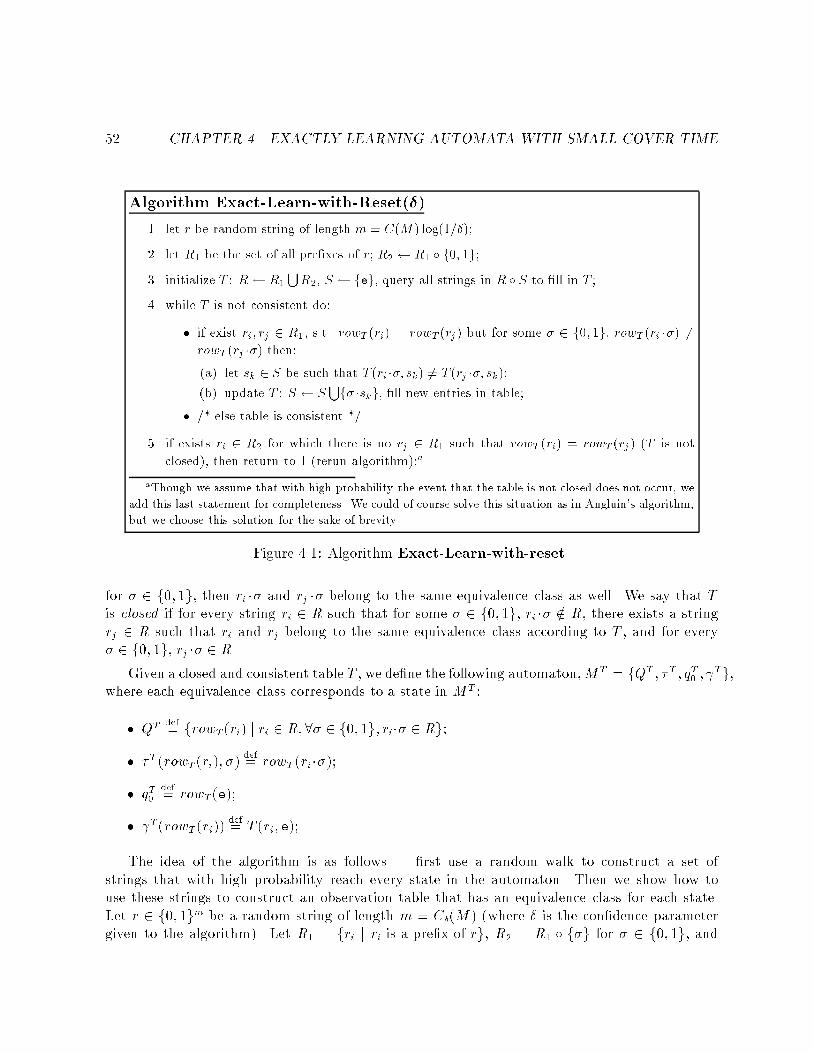
52 CHAPTER 4. EXACTLY LEARNING AUTOMATA WITH SMALL COVER TIMEAlgorithm Exact-Learn-with-Reset(�)1. let r be random string of length m = C(M ) log(1=�);2. let R1 be the set of all pre�xes of r; R2 R1 � f0; 1g;3. initialize T : R R1SR2, S feg, query all strings in R � S to �ll in T ;4. while T is not consistent do:� if exist ri; rj 2 R1, s.t. rowT (ri) = rowT (rj) but for some � 2 f0; 1g, rowT (ri ��) 6=rowT (rj ��) then:(a) let sk 2 S be such that T (ri ��; sk) 6= T (rj ��; sk);(b) update T : S SSf� �skg, �ll new entries in table;� /* else table is consistent */5. if exists ri 2 R2 for which there is no rj 2 R1 such that rowT (ri) = rowT (rj) (T is notclosed), then return to 1 (rerun algorithm);aaThough we assume that with high probability the event that the table is not closed does not occur, weadd this last statement for completeness. We could of course solve this situation as in Angluin's algorithm,but we choose this solution for the sake of brevity.Figure 4.1: Algorithm Exact-Learn-with-resetfor � 2 f0; 1g, then ri �� and rj �� belong to the same equivalence class as well. We say that Tis closed if for every string ri 2 R such that for some � 2 f0; 1g, ri �� =2 R, there exists a stringrj 2 R such that ri and rj belong to the same equivalence class according to T , and for every� 2 f0; 1g, rj �� 2 R.Given a closed and consistent table T , we de�ne the following automaton,MT = fQT ; �T ; qT0 ; Tg,where each equivalence class corresponds to a state in MT :� QT def= frowT(ri) j ri 2 R; 8� 2 f0; 1g; ri�� 2 Rg;� �T (rowT(ri); �) def= rowT (ri��);� qT0 def= rowT(e);� T(rowT(ri)) def= T (ri; e);The idea of the algorithm is as follows | �rst use a random walk to construct a set ofstrings that with high probability reach every state in the automaton. Then we show how touse these strings to construct an observation table that has an equivalence class for each state.Let r 2 f0; 1gm be a random string of length m = C�(M) (where � is the con�dence parametergiven to the algorithm). Let R1 = fri j ri is a pre�x of rg, R2 = R1 � f�g for � 2 f0; 1g, and

4.2. EXACT LEARNING WITH A RESET 53R = R1SR2. The learning algorithm initializes S to include only the empty string, e, and �lls inthe (single columned) table by performing membership queries. Let us �rst observe that from thede�nition of C�(M), we have that with probability at least 1��, for every state q 2 Q, there existsa string ri 2 R1, such that �(q0; ri) = q. Assume that this is in fact the case. It directly followsthat T is always closed. Hence, the learning algorithm must only ensure that T be consistent.This is done as follows. If there exists a pair of strings ri; rj 2 R such that rowT(ri) = rowT(rj),but for some � 2 f0; 1g, rowT(ri��) 6= rowT (rj��), then a string ��sk is added to S, where sk 2 Sis such that T (ri ��; sk) 6= T (rj ��; sk), and the new entries in T are �lled in. The pseudo-code forthe algorithm appears in Figure 4.1.It is clear that the inconsistency resolving process (stage 4 in the algorithm given in Figure 4.1)ends after at most n � 1 steps. This is true since every string added to S re�nes the partitioninduced by T . On the other hand, the number of equivalence classes cannot exceed n, since forevery pair of strings ri; rj 2 R such that rowT (ri) 6= rowT(rj), ri and rj reach two di�erent statesin M . The running time of the algorithm is hence at most 3nC(M) log(1=�). We further makethe following claim:Lemma 4.2.1 If for every state q 2 Q, there exists a string ri 2 R1 such that �(q0; ri) = q, thenMT �M .Proof: Let � : Q! QT be de�ned as follows: for each q 2 Q, �(q) = T (ri), where ri 2 R is suchthat �(q0; ri) = q. From the assumption in the statement of the lemma we have that for everystate q 2 Q, there exists a string ri 2 R1 such that �(q0; ri) = q. By de�nition of deterministic�nite automata, if for ri 6= rj in R, �(q0; ri) = �(q0; rj), then necessarily T (ri) = T (rj). It followsthat � is well de�ned. We next show that � satis�es the following properties:1. �(q0) = qT0 ;2. 8q 2 Q, 8� 2 f0; 1g, �(�(q; �)) = �T (�(q); �);3. 8q 2 Q; (q) = T(�(q))If � has the above properties, then for every string s 2 f0; 1g�, (�(q0; s)) = T(�T (qT0 ; s)), andthe claim follows.� has the �rst property since �(q0; e) = q0, and qT0 def= T (e). � has the third property since T(T (ri)) def= T (ri; e) =M(ri) = (�(q0; ri)). It remains to prove the second property. Let ri 2 R1be such that �(q0; ri) = q. From the assumption in the statement of the lemma, we know thereexists such a string. Thus, �(q) = T (ri). By de�nition of MT , �T (T (ri); �) = T (ri ��). Since�(q0; ri) = q, we have that �(q; �) = �(q0; ri ��), and by de�nition of �, �(�(q; �)) = T (ri ��) =�T (T (ri); �).Note that if M is irreducible in the sense that for every pair of states q; q0 2 Q, there exists astring s of length at most n, such that the label of �(q; s) di�ers from the label of �(q0; s), then �is an isomorphism.

54 CHAPTER 4. EXACTLY LEARNING AUTOMATA WITH SMALL COVER TIMEWe thus have the following theorem.Theorem 4.1 For every target automaton M , if C(M) = poly(n), then the running time ofExact-Learn-with-Reset is poly(n; log(1=�)), and with probability at least 1 � � it outputs a hy-pothesis DFA which is equivalent to M .4.3 Exact Learning without a ResetIn this section we describe an exact learning algorithm (as de�ned in Subsection 2.4) for automatawhose cover time is polynomial in their size. This algorithm closely follows Rivest and Schapire'slearning algorithm [RS93]. However, we use new techniques that exploit the small cover time ofthe automaton in place of relying on a teacher who supplies us with counterexamples to incorrecthypotheses.As in [RS93], we overcome the absence of a reset by the use of a homing sequence, de�nedbelow.Definition 4.3.1 A homing sequence h 2 f0; 1g�, is a sequence of symbols such that for everypair of states q1; q2 2 Q, if q1hhi = q2hhi, then �(q1; h) = �(q2; h).It is not hard to verify (cf. [Koh78]) that every DFA has a homing sequence of length at mostquadratic in its size. Moreover, given the DFA, such a homing sequence can be found e�ciently.Assume we had a homing sequence h for our target DFA M (we shall of course remove thisassumption shortly). Then we would create at most n copies of the algorithm Exact-Learn-with-Reset , ELR�1 ; : : : ; ELR�n, each corresponding to a di�erent output sequence �i of the homingsequence, and hence to a di�erent e�ective starting state. At each stage, the algorithm walksaccording to the homing sequence, observing the output sequence �, and then simulates the nextstep of ELR�. The algorithm terminates when one of these copies completes. If we run eachcopy of Exact-Learn-with-Reset with the con�dence parameter �=n, then using Theorem 4.1, withprobability at least 1 � � the hypothesis of the completed copy is correct, and the running timeof the algorithm is at most n4C(M) log(n=�). Details of the algorithm are given in Figure 4.2.If h is unknown, consider the case in which we guess a sequence h0 which is not a homingsequence and run the algorithm Exact-Learn-Given-Homing-Sequence with h0 instead of h. Sinceh0 is not a homing sequence, there exist two states q1 6= q2, such that for some pair of statesq01; q02, a walk starting at q01 reaches q1 upon executing h0 and a walk starting at q02 reaches q2 uponexecuting h0, but the output sequence in both cases is the same. Therefore, when we simulate thecopy ELR�, some of the queries (walks) might be performed starting from q1, and some mightbe performed starting from q2.There are two possible consequences to such an event. The �rst is that the algorithm discoversthat there is no single starting state corresponding to the observation table T�. This can bediscovered either by observing two di�erent outputs when performing the same walk (which

4.3. EXACT LEARNING WITHOUT A RESET 55Algorithm Exact-Learn-Given-Homing-Sequence(�)� while no copy of Exact-Learn-with-Reset has completed do:1. perform the walk corresponding to h, and let � be the corresponding output sequence;2. if there does not exist a copy ELR� of Exact-Learn-with-Reset(�=n), then createsuch a new copy;3. simulate the next query of ELR� by performing the corresponding walk;4. if the observation table T� of ELR� is consistent and closed then output MT� ;/* ELR� has completed */5. if T� is consistent but not closed, then discard ELR�;Algorithm Exact-Learn(�)1. h e;2. while no copy of Exact-Learn-with-Reset-R is completed do:(a) choose uniformly and at random a length ` 2 [0; : : : ; C�(M )], and then perform arandom walk of length `.(b) perform the walk corresponding to h, and let � be the corresponding output sequence;(c) if there does not exist a copy ELRR� of Exact-Learn-with-Reset-R(�=(2n2)), thencreate such a new copy;(d) simulate the next query w of ELRR� by performing the corresponding walk;(e) if the answer to w is di�erent from a previous answer to w, then do:i. h h�w;ii. discard all existing copies of Exact-Learn-with-Reset-R, and go to 2; /* restartalgorithm with extended h */(f) if the observation table T� of ELRR� is consistent and closed then output MT� ; /*ELRR� has completed */(g) if T� is consistent but not closed, then discard ELRR�;Figure 4.2: Algorithm Exact-Learn-Given-Homing-Sequence and Algorithm Exact-Learn

56 CHAPTER 4. EXACTLY LEARNING AUTOMATA WITH SMALL COVER TIMEmight happen when the algorithm asks two queries such that one is a pre�x of the other), orif the number of columns in T� is greater than n. In the �rst case we have found a sequencewhose output distinguishes between q1 and q2, and in the second case, we can use a probabilisticprocedure proposed by Rivest and Schapire [RS93] to �nd such a distinguishing sequence. In bothcases we can simply extend h0 by the distinguishing sequence found and restart the algorithm withthe \improved" h0. Clearly, h0 can be extended in this manner at most n�1 times before it becomesa true homing sequence, whose total length is at most (n� 1)(C(M) log(n=�)+n) plus the initiallength of h0.The second possible consequence is that the observation table T� becomes consistent andclosed, but the hypothesis MT� is incorrect . This may occur since di�erent entries correspond toqueries answered from di�erent e�ective starting states. If the learning algorithm had access toa teacher who would supply it with a counterexample to its incorrect hypothesis, then it couldextend h0 by the counterexample and proceed as described above. In what follows we describehow to modify the algorithm so that it constructs a (true) homing sequence without the aid ofa teacher. The pseudocode for the algorithm appears in Figure 4.2. It is interesting to notethat the (tempting) idea to try and randomly guess a counterexample does not work even in thecase of automata that have small cover time. Rivest and Zuckerman [RZ92] construct a pair ofautomata which both have small cover time, but for which the probability of randomly guessinga distinguishing sequence is exponentially small. These automata are described in Appendix B.We now show how we can avoid the second possible consequence and discover whether acopy of ELR� is simulated from several e�ective starting states. We de�ne the algorithm Exact-Learn-with-Reset-R to be a variant of Exact-Learn-with-Reset, in which each query is repeated Nconsecutive times, where N is set subsequently. Suppose that instead of simulating copies ELR�of Exact-Learn-with-Reset, as in Exact-Learn-Given-Homing-Sequence, we simulate copies ELRR�of Exact-Learn-with-Reset-R. If we �nd that for the same query w, we get two di�erent answers(in two di�erent simulations of some ELRR�), then we know that h is not a homing sequence,and thus we extend h by w, and restart the algorithm.3 We would like to ensure, that with highprobability, if a copy ELRR� corresponds to more than one starting state, and there are two ofthese starting states that disagree on some entry in T�, then we shall discover it.For a candidate homing sequence h, let Q� be the set of states reached upon executing h andobserving �. Namely, Q� def= fq : q 2 Q; 9q0 s.t. q0hhi = �g :For a state q 2 Q� , let B(q) be the set of states from which q is reached upon executing h, i.e.,B(q) def= fq0 : q0 2 Q; �(q0; h) = qg :3As in [RS93], we actually need not discard all copies and restart the algorithm, but we may only discard thecopy in which the disagreement was found, and construct an adaptive homing sequence which results in a moree�cient algorithm. For sake of simplicity of this presentation, we continue with the use of the less e�cient, presethoming sequence.

4.3. EXACT LEARNING WITHOUT A RESET 57We would like to guarantee, that with high probability, for every query to �ll an entry in T�, andfor every q 2 Q� , one of the N repetitions of the query is executed starting from q. To this end wedo the following. Each time before we execute h, we randomly choose a length 0 � ` � C�(M),and perform a random walk of length `. The idea behind this random walk is that for every statethere is some non-negligble probability of reaching it upon performing the random walk.For some entry (ri; sj) in T� , consider the N executions of h whose outcome was � and whichwere followed by the simulation of the query ri�sj . For a given q 2 Q�, we bound the probabilitythat we did not reach q after any one of the N executions of h as follows. Assume that insteadof choosing a random length and performing a random walk of that length, we �rst randomlychoose a string t of length C�(M), then choose a random length `, and �nally perform a walkcorresponding to the length ` pre�x of t. Clearly the distribution on the states reached at theend of this walk is equivalent to the distribution on the states reached by the original randomizedprocedure. Thus, the probability that we did not reach some q 2 Q� is at mostN�+ (1� 1=C�(M))N : (4.1)The �rst term is a bound on the probability that for at least one of the random strings t, none ofthe states in B(q) are passed on the walk corresponding to t. Given that such an event does notoccur, the second term is a bound on the probability that none of the pre�xes chosen reach anyof these states.It remains to set � and N . Since we simulate at most n2 copies ELRR� during the completerun of the algorithm, each with the parameter �=(2n2), then with probability at least 1 � �=2,each copy has a row in its observation table which corresponds to each state in Q. It follows(Lemma 4.2.1) that when h �nally turns into a homing sequence (after at most n� 1 extensions),and some table T� becomes consistent, then MT� is a correct hypothesis.For each of the possible n2 copies ELRR�, the number of entries in the observation table T�is at most nC(M) log(2n2=�). If we choose N and � so thatN�+ (1� 1=(C(M) log(1=�))N < �=(2n3C(M) log(2n2=�)) ; (4.2)then with probability at least 1 � �=2, we do not output a hypothesis of a copy ELRR� whichcorresponds to more than one e�ective starting state (unless the di�erent starting states areequivalent). The following choice gives us the required bound:N = C(M) log 4n3C(M) log 2n2�� !� log2 C(M) log 4n3C(M) log 2n2�� !! ;� = �4Nn3C(M) log 2n2� :We have thus proven that:Theorem 4.2 Algorithm Exact-Learn is an exact learning algorithm for automata whose covertime is polynomial in n.

58 CHAPTER 4. EXACTLY LEARNING AUTOMATA WITH SMALL COVER TIME4.4 Exact Learning in the Presence of NoiseAlgorithm Exact-Noisy-Learn(�)1. h e;2. while no copy of Exact-Noisy-Learn-with-Reset is completed do:(a) � Execute-Homing-Sequence(h);(b) if there does not exist a copy ENLR� of Exact-Noisy-Learn-with-Reset(�=(2n2)),then create such a new copy;(c) simulate the next query w of ENLR� by performing the corresponding walk; let �i(w)be the output of the state reached, where i is the number of times w has been queried.(d) if i = N then let f(w) = (1=N )PNi=1 �i(w). If jf(w)� �j > �, and jf(w)� (1� �)j > �then do:i. h h�w;ii. discard all existing copies of Exact-Noisy-Learn-with-Reset, and go to (2); /*restart algorithm with extended h */(e) if the observation table T� of ENLR� is consistent and closed then output MT� ; /*ENLR� has completed */(f) if T� is consistent but not closed, then discard ENLR�;Figure 4.3: Algorithm Exact-Noisy-LearnIn this section we describe how to modify the learning algorithm described in Section 4.3 inorder to overcome a noisy environment. Some of the parameters are not explicitly set, but can beeasily derived using standard Cherno� bounds. We name the new algorithm Exact-Noisy-Learn,and its pseudo-code appears in Figure 4.3.We �rst observe that � can easily be approximated within a small additive error �, and withprobability at least 1��=2, in time polynomial in n, 1=�, log 1=�, and 1=�. This can be done usinga method similar to the one described in [RR95] (see Appendix E, Subsection E.5.1). The ideaused is as follows. Consider a pair of strings w1 and w2. For a string z, let the behavior of wi on zbe the output observed by the learner after executing the walk corresponding to wi�z, and let thecorrect behavior of wi on z be the (correct) output of the state reached after executing the walkcorresponding to wi�z. If w1 and w2 reach the same state, then for every string z, w1�z and w2�zalso reach the same state. Thus, the di�erence in the behavior of w1 and w2 on any set of stringsis entirely due to the noise process. If w1 and w2 reach di�erent states, then their di�erence inbehavior on a set of strings Z is due to the di�erence in the correct behavior of the strings on Zas well as the noise. Thus in order to estimate the noise rate, we look for two strings that reachthe same state and estimate the di�erence in their behavior. This can be done as follows.Let t be an arbitrary string of length L. Suppose t is executed n+1 times, and for 1 � i � n+1,

4.4. EXACT LEARNING IN THE PRESENCE OF NOISE 59let qi be the state reached after performing t exactly i � 1 times and let oi = oi1 : : : oiL be thesequence of outputs corresponding to the ith execution of t. Clearly, for some pair of indicesi 6= j, qi = qj . For every pair 1 � i < j � n + 1, let dij = 1LPLk=1 oik � ojk. De�ne dmin to bethe minimum value over all such pairs, and let � < 1=2 be the solution of the quadratic equation2�(1� �) = dmin. If qi = qj , then E[dij] = 2�(1� �). It can easily be veri�ed that if qi 6= qj , thenE[dij] � 2�(1� �). We can thus apply Hoe�ding's inequality (Inequality 1) to derive an upperbound on jdmin � 2�(1� �)j as a function of L, which implies an upper bound on j� � �j.4 Wethus assume from here on, that we have a good approximation, �, of �.Procedure Execute-Homing-Sequence(h)1. choose uniformly and at random a length ` 2 [0; : : : ; C�(M )], and then perform a randomwalk of length `.2. perform the walk corresponding to h for m consecutive times, and for 1 � i � m, let oi bethe output sequence corresponding to the ith execution of h;3. for each length 1 � v � n, and for every 1 � j � jhj, let vj = 1=mvPmvk=1 om�kvj , wheremv = bm=vc;4. let v be such that for every j either j vj � �j � �, or j vj � (1� �)j � �; if there is no such v,then return to (1);5. for 1 � j � jhj, let �j = 1 if jv > 1=2, and 0 otherwise;6. return �; Figure 4.4: Procedure Execute-Homing-SequenceAs in the noise free case, we �rst assume that the algorithm has means of a reset. With thisassumption, we use the technique of [Sak91] and de�ne a slight modi�cation of Exact-Learn-with-Reset, named Exact-Noisy-Learn-with-Reset, which simply repeats each query N times, and �lls thecorresponding entry in the table with the majority observed label. Thus, with high probability,for an appropriate choice of N , the majority observed label is in fact the correct label of thequeried string.Next we assume that the algorithm has no means of a reset, but instead, has a homingsequence, h. Clearly, in a single execution of h, with high probability, the output sequence will beerroneous. We thus adapt a technique that was used in [DAB+95]. Assume we execute the homingsequence m consecutive times, where m >> n. The last m�n executions of the homing sequencemust be following a cycle. We use this fact to estimate the output sequence corresponding tothe last homing sequence executed. For 1 � i � m, let qi be the state reached after the ithexecution of h. Let oi = oi1 : : : oijhj be the output sequence corresponding to this execution, andlet bp = b(m� n)=pc. Then there exists some (minimal) period p, where 1 � p � n, such that forevery 1 � k � bp, qm = qm�kp. For every 1 � j � jhj we let �j = 1 if 1=bpPbpk=1 om�kvj > 1=2, and4For a more detailed analysis, see Appendix E, Subsection E.5.1.

60 CHAPTER 4. EXACTLY LEARNING AUTOMATA WITH SMALL COVER TIME0 otherwise. It follows that with high probability, for an appropriate choice of m, the sequence� = �1 : : :�jhj is the correct output sequence corresponding to the last execution of h. In thiscase we could proceed as in Exact-Learn-Given-Homing-Sequence, simulating copies of Exact-Noisy-Learn-with-Reset, instead of copies of Exact-Learn-with-Reset.How do we �nd the period p? For each possible length 1 � v � n, let bv = b(m� n)=vc, andlet ~ v be an jhj dimensional vector which is de�ned as follows. For 1 � j � jhj, vj = 1=bv bvXk=1 om�kvj : (4.3)Let qij be the state reached after i executions of h, followed by the length j pre�x of h. Whenv = p, then by de�nition of p for every k; k0, and for every j, qm�kvj = qm�k0vj . Therefore, withhigh probability, for every j, vj is either within � of 1� �, or within � of �, for some small additiveerror �.When v 6= p, then there are two possibilities. If for every j and for every k; k0, (qm�kvj ) = (qm�k0vj ) (even though qm�kvj might di�er from qm�k0vj ), then the following is still true. De�ne �vjto be 1 if vj is greater than 1=2, and 0 if it is at most 1=2. Then �v is the correct output sequencecorresponding to the last execution of h. Otherwise, let j be an index for which the above doesnot hold, and let K0 = fk j (qm�kvj ) = 0g, and K1 = fk j (qm�kvj ) = 1g. We claim that bothK0=bv and K1=bv are at least 1=p which is at least 1=n. This is true since v � p must be a periodas well, and hence for every k and k0 which are multiples of v � p, qm�kvj = qm�k0vj . It follows thatE[ vj ] = �(1� �) + (1� �)� (4.4)where � = K1=bv. Since 1=n � � � 1� 1=n,� + (1� 2�) 1n � E[ vj ] � (1� �)� (1� 2�) 1n :Using this bound on the expected value of vj , we have that the observed value of vj is boundedaway from both � and 1� � with high probability. Therefore, since � is a good approximation to�, we are able to detect whether or not v = p.For an appropriate choice of m we can thus infer the correct output sequence correspondingto the homing sequence h (or any other given sequence). The pseudo-code for the proceduredescribed above appears in Figure 4.4.It remains to treat the case in which a homing sequence is not known. Similarly to the noisefree case, for a (correct) output sequence � corresponding to a candidate homing sequence h,let Q� be all states q 2 Q for which there exists a state q0 2 Q such that q0hhi = �. For astate q 2 Q� , let B(q) be the set of states q0 such that �(q0; hm) = q. Let (ri; sj) be an entryin the table for which there exist q1; q2 2 Q� , such that (�(q1; ri �sj)) 6= (�(q2; ri �sj)). LetQ1� = fq j q 2 Q�; (�(q1; ri �sj)) = 1g, and let Q0� be de�ned similarly. If, as in the noise freecase, the query ri �sj is repeated N times, and a random walk of some length ` � kC(M) is

4.4. EXACT LEARNING IN THE PRESENCE OF NOISE 61performed prior to the m executions of h, then with high probability the fraction of times a stateq 2 Q1�(Q0�) is reached is at least 1=kC(M). As in the analysis above for identifying a length vwhich is not a period, we can identify that we have a mixture of more than one starting state,and extend h by ri�sj.The above discussion constitutes a proof of the following theorem:Theorem 4.3 Algorithm Exact-Noisy-Learn is an exact learning algorithm in the presence of noisefor automata whose cover time is polynomial in n.

62 CHAPTER 4. EXACTLY LEARNING AUTOMATA WITH SMALL COVER TIME

Part IIProbabilistic Automata

63

Chapter 5Learning Probabilistic Automatawith Variable Memory Length5.1 IntroductionStatistical modeling of complex sequences is a fundamental goal of machine learning due to its widevariety of natural applications. The most noticeable examples of such applications are statisticalmodels in human communication such as natural language, handwriting and speech [Jel85, Nad84],and statistical models of biological sequences such as DNA and proteins [KMH93].These kinds of complex sequences clearly do not have any simple underlying statistical sourcesince they are generated by natural sources. However, they typically exhibit the following sta-tistical property, which we refer to as the short memory property. If we consider the (empirical)probability distribution on the next symbol given the preceding subsequence of some given length,then there exists a length L (the memory length), such that the conditional probability distribu-tion does not change substantially if we condition it on preceding subsequences of length greaterthan L.This observation suggests modeling such sequences by Markov chains of order L > 1, (alsoknown as n-gram models [Sha51]) where the order is the memory length of the model. Alter-natively, such sequences are often modeled by Hidden Markov Models (HMM) which are morecomplex distribution generators and hence may capture additional properties of natural sequences.These statistical models de�ne rich families of sequence distributions and moreover, they give ef-�cient procedures both for generating sequences and for computing their probabilities. However,both models have severe drawbacks. The size of Markov chains grows exponentially with theirorder, and hence only very low order Markov chains can be considered in practical applications.Such low order Markov chains might be very poor approximators of the relevant sequences. Inthe case of HMM's, there are known hardness results concerning their learnability which were65

66 CHAPTER 5. LEARNING PROB. AUTOMATA WITH VARIABLE MEMORYdiscussed in Subsection 1.2.2.In this chapter we propose a simple stochastic model and describe its learning algorithm. Weprove that the algorithm is e�cient and demonstrate its applicability to several practical modelingproblems. It has been observed that in many natural sequences, the memory length depends onthe context and is not �xed . The model we suggest is hence a variant of order LMarkov chains, inwhich the order, or equivalently, the memory, is variable. We describe this model using a subclassof Probabilistic Finite Automata (PFA), which we name Probabilistic Su�x Automata (PSA).Each state in a PSA is labeled by a string over an alphabet �. The transition function betweenthe states is de�ned based on these string labels, so that a walk on the underlying graph of theautomaton, related to a given sequence of length at least L, always ends in a state labeled by asu�x of the sequence. The lengths of the strings labeling the states are bounded by some upperbound L, but di�erent states may be labeled by strings of di�erent length, and are viewed ashaving varying memory length. When a PSA generates a sequence, the probability distributionon the next symbol generated is completely de�ned given the previously generated subsequenceof length at most L. Hence, as mentioned above, the probability distributions these automatagenerate can be equivalently generated by Markov chains of order L, but the description using aPSA may be much more succinct. Since the size of an order L markov chains is exponential in L,their estimation requires data length and time exponential in L.In our learning model we assume that the learning algorithm is given a sample (consistingeither of several sample sequences or of a single sample sequence) generated by an unknowntarget PSA M of some bounded size. The algorithm is required to output a hypothesis machineM , which is not necessarily a PSA but which has the following properties. M can be used both toe�ciently generate a distribution which is a good approximation of the one generated by M , andgiven any sequence s, it can e�ciently compute the probability assigned to s by this distribution.Several measures of the quality of a hypothesis can be considered. Since we are mainly interestedin models for statistical classi�cation and pattern recognition, the most natural measure is theKullback-Leibler (KL) divergence. Our results hold equally well for the variation (L1) distance andother norms, which are upper bounded by the KL-divergence. Since the KL-divergence betweenMarkov sources grows linearly with the length of the sequence, the appropriate measure is theKL-divergence per symbol. An �-good hypothesis thus has at most � KL-divergence per symbolto the target.In particular, the hypothesis our algorithm outputs, belongs to a class of probabilistic machinesnamed Probabilistic Su�x Trees (PST). The learning algorithm grows such a tree starting froma single root node, and adaptively adds nodes (strings) for which there is strong evidence in thesample that they signi�cantly a�ect the prediction properties of the tree. We show that everydistribution generated by a PSA can equivalently be generated by a PST that is not much larger.We also show and that for every PST there exists an equivalent PFA which is not much largerand which is a slight variant of a PSA. There are some contexts in which PSA's are preferable,and some in which PST's are preferable, and therefore we use both representation in the chapter.For example, PSA's are more e�cient generators of distributions, and since they are probabilistic

5.2. PRELIMINARIES 67automata, there is a natural notion of the stationary distribution on the states of a PSA whichPST's lack. On the other hand, PST's sometimes have more succinct representations than theequivalent PSA's, and there is a natural notion of growing them.Stated formally, our main theoretical result is the following. If both a bound L, on thememory length of the target PSA, and a bound n, on the number of states the target PSA has,are known, then for every given 0 < � < 1 and 0 < � < 1, our learning algorithm outputsan �-good hypothesis PST with con�dence 1 � �, in time polynomial in L, n, j�j, 1� and 1� .Furthermore, such a hypothesis can be obtained from a single sample sequence if the sequencelength is also polynomial in a parameter related to the rate in which the target machine convergesto its stationary distribution. Thus, despite an intractability result concerning the learnability ofdistributions generated by Probabilistic Finite Automata (which is described in Section 6.3), ourrestricted model can be learned in a PAC-like sense e�ciently.Overview of the chapterThis chapter is organized as follows. In Section 5.2 we give some de�nitions and notation anddescribe the families of distributions studied in this chapter, namely those generated by PSA's andthose generated by PST's. In Section 5.3 we discuss the relation between the above two familiesof distributions. In Section 5.4 the learning algorithm is described. Some of the proofs regardingthe correctness of the learning algorithm are given in Section 5.5. Finally, we demonstrate theapplicability of the algorithm by two illustrative examples in Section 5.6. In the �rst example weuse our algorithm to learn the structure of natural English text, and use the resulting hypothesisfor correcting corrupted text. In the second example we use our algorithm to build a simplestochastic model for E.coli DNA. The detailed proofs of the claims presented in Section 5.3 con-cerning the relation between PSA's and PST's are provided in Appendix C, Sections C.1 and C.2.The more technical proofs and lemmas regarding the correctness of the learning algorithm aregiven in Section C.3.5.2 Preliminaries5.2.1 Probabilistic Su�x AutomataWe are interested in learning a subclass of PFA's which we name Probabilistic Su�x Automata(PSA). These automata have the following property. Each state in a PSAM is labeled by a stringof �nite length in ��. The set of strings labeling the states is su�x free. For every two statesq1; q2 2 Q and for every symbol � 2 �, if �(q1; �) = q2 and q1 is labeled by a string s1, then q2 islabeled by a string s2 which is a su�x of s1 ��. In order that � be well de�ned on a given set ofstrings S, not only must the set be su�x free, but it must also have the following property. Forevery string s in S labeling some state q, and every symbol � for which (q; �) > 0, there exists

68 CHAPTER 5. LEARNING PROB. AUTOMATA WITH VARIABLE MEMORYa string in S which is a su�x of s�. For our convenience, from this point on, if q is a state in Qthen q will also denote the string labeling that state.We require that the underlying graph of M , de�ned by Q and �(�; �), be strongly connected ,i.e., for every pair of states q and q0 there must be a directed path from q to q0. Note that in ourde�nition of PFA's in Section 2.3 we assumed that the probability associated with each transition(edge in the underlying graph) is non-zero, and hence, strong connectivity implies that every statecan be reached from every other state with non-zero probability. For simplicity we assume M isaperiodic, i.e., that the greatest common divisor of the lengths of the cycles in its underlying graphis 1. These two requirements ensure us that M is ergodic, namely that there exists a distribution�M on the states, such that for every state we may start at, the probability distribution on thestate reached after time t as t grows to in�nity, is �M . The probability distribution �M is theunique distribution satisfying�M(q = s1 : : : sl) = Xq0 s:t: �(q0;sl)=q�M(q0) (q0; sl) ; (5.1)and is named the stationary distribution of M . We ask that for every state q in Q, the initialprobability of q, �(q), be the stationary probability of q, �M(q). It should be noted that therequirements above are needed only when learning from a single sample string and not whenlearning from many sample strings. However, for sake of brevity we make these requirements inboth cases.For any given L � 0, the subclass of PSA's in which each state is labeled by a string of lengthat most L is denoted by L-PSA. An example 2-PSA is depicted in Figure 5.1. A special case ofthese automata is the case in which Q includes all strings in �L. An example of such a 2-PSAis depicted in Figure 5.1 as well. These automata can be described as Markov chains of order L.The states of the Markov chain are the symbols of the alphabet �, and the next state transitionprobability depends on the last L states (symbols) traversed. Since every L-PSA can be extendedto a (possibly much larger) equivalent L-PSA whose states are labeled by all strings in �L, it canalways be described as a Markov chain of order L. Alternatively, since the states of an L-PSAmight be labeled by only a small subset of ��L, and many of the su�xes labeling the states maybe much shorter than L, it can be viewed as a Markov chain with variable order, or variablememory.Learning Markov chains of order L, i.e., L-PSA's whose states are labeled by all �L strings,is straightforward (though it takes time exponential in L). Since the \identity" of the states (i.e.,the strings labeling the states) is known, and since the transition function � is uniquely de�ned,learning such automata reduces to approximating the next symbol probability function . Forthe more general case of L-PSA's in which the states are labeled by strings of variable length, thetask of an e�cient learning algorithm is much more involved since it must reveal the identity ofthe states as well.

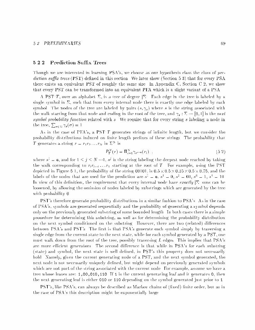
5.2. PRELIMINARIES 695.2.2 Prediction Su�x TreesThough we are interested in learning PSA's, we choose as our hypothesis class the class of pre-diction su�x trees (PST) de�ned in this section. We later show (Section 5.3) that for every PSAthere exists an equivalent PST of roughly the same size. In Appendix C, Section C.2, we showthat every PST can be transformed into an equivalent PFA which is a slight variant of a PSA.A PST T , over an alphabet �, is a tree of degree j�j. Each edge in the tree is labeled by asingle symbol in �, such that from every internal node there is exactly one edge labeled by eachsymbol. The nodes of the tree are labeled by pairs (s; s) where s is the string associated withthe walk starting from that node and ending in the root of the tree, and s : �! [0; 1] is the nextsymbol probability function related with s. We require that for every string s labeling a node inthe tree, P�2� s(�) = 1.As in the case of PFA's, a PST T generates strings of in�nite length, but we consider theprobability distributions induced on �nite length pre�xes of these strings. The probability thatT generates a string r = r1r2 : : : rN in �N isPNT (r) = �Ni=1 si�1(ri) ; (5.2)where s0 = e, and for 1 � j � N � 1, sj is the string labeling the deepest node reached by takingthe walk corresponding to riri�1 : : :r1 starting at the root of T . For example, using the PSTdepicted in Figure 5.1, the probability of the string 00101, is 0:5� 0:5� 0:25� 0:5� 0:75, and thelabels of the nodes that are used for the prediction are s0 = e; s1 = 0; s2 = 00; s3 = 1; s4 = 10.In view of this de�nition, the requirement that every internal node have exactly j�j sons can beloosened, by allowing the omission of nodes labeled by substrings which are generated by the treewith probability 0.PST's therefore generate probability distributions in a similar fashion to PSA's. As in the caseof PSA's, symbols are generated sequentially and the probability of generating a symbol dependsonly on the previously generated substring of some bounded length. In both cases there is a simpleprocedure for determining this substring, as well as for determining the probability distributionon the next symbol conditioned on the substring. However, there are two (related) di�erencesbetween PSA's and PST's. The �rst is that PSA's generate each symbol simply by traversing asingle edge from the current state to the next state, while for each symbol generated by a PST, onemust walk down from the root of the tree, possibly traversing L edges. This implies that PSA'sare more e�cient generators. The second di�erence is that while in PSA's for each substring(state) and symbol, the next state is well de�ned, in PST's this property does not necessarilyhold. Namely, given the current generating node of a PST, and the next symbol generated, thenext node is not necessarily uniquely de�ned, but might depend on previously generated symbolswhich are not part of the string associated with the current node. For example, assume we have atree whose leaves are: 1,00,010,110. If 1 is the current generating leaf and it generates 0, thenthe next generating leaf is either 010 or 110 depending on the symbol generated just prior to 1.PST's, like PSA's, can always be described as Markov chains of (�xed) �nite order, but as inthe case of PSA's this description might be exponentially large.

70 CHAPTER 5. LEARNING PROB. AUTOMATA WITH VARIABLE MEMORYWe shall sometimes want to discuss only the structure of a PST and ignore its predictionproperty. In other words, we will be interested only in the string labels of the nodes and not inthe values of s(�). We refer to such trees as su�x trees. We now introduce two more notations.The set of leaves of a su�x tree T is denoted by L(T ), and for a given string s labeling a node vin T , T (s) denotes the subtree rooted at v.CCCCCCCCCCCCCCCCCCCCCCCCCCCCCCCCCCCCCCCCCC

00

CCCCCCCCCCCCCCCCCCCCCCCCCCCCCCCCCCCCCCCCCCCCCCCCC

1

CCCCCCCCCCCCCCCCCCCCCCCCCCCCCCCCCCCCCCCCCC

10

0.5

0.5

0.75

0.75

0.25

0.25

π(1)=0.5

π(00)=0.25π(10)=0.25

CCCCCCCCCCCCCCCCCCCCCCCCCCCCCCCCCCCCCCCCCC

00

CCCCCCCCCCCCCCCCCCCCCCCCCCCCCCCCCCCCCCCCCC

π(00)=0.25π(10)=0.25

0.5

CCCCCCCCCCCCCCCCCCCCCCCCCCCCCCCCCCCCCCCCCC

CCCCCCCCCCCCCCCCCCCCCCCCCCCCCCCCCCCCCCCCCC

10

11 010.5

0.50.5

0.25

0.250.75

0.75

π(11)=0.25 π(01)=0.25

CCCCCCCCCCCCCCCCCCCCCCCCCCCCCCCCCCCCCCCCCC

CCCCCCCCCCCCCCCCCCCCCCCCCCCCCCCCCCCCCCCCCC

CCCCCCCCCCCCCCCCCCCCCCCCCCCCCCCCCCCCCCCCCC

CCCCCCCCCCCCCCCCCCCCCCCCCCCCCCCCCCCCCCCCCC

CCCCCCCCCCCCCCCCCCCCCCCCCCCCCCCCCCCCCCCCCC

e

0 1

00 10

(0.5,0.5)

(0.5,0.5)(0.5,0.5)

(0.25,0.75)(0.75,0.25)Figure 5.1: Left: A 2-PSA. The strings labeling the states are the su�xes corresponding to them.Bold edges denote transitions with the symbol `1', and dashed edges denote transitions with `0'.The transition probabilities are depicted on the edges. Middle: A 2-PSA whose states are labeledby all strings in f0; 1g2. The strings labeling the states are the last two observed symbols beforethe state was reached, and hence it can be viewed as a representation of a Markov chain of order 2.It is equivalent to the (smaller) 2-PSA on the left. Right: A prediction su�x tree. The predictionprobabilities of the symbols `0' and `1', respectively, are depicted beside the nodes, in parentheses.5.2.3 The Learning ModelThe main features of the learning model under which we present our results in this chapter wherepresented in Section 2.5. Here we describe some additional details which were not presented inthat section. In addition to the parameters � and �, we assume that a learning algorithm forPSA's is given the maximum length L of the strings labeling the states of the target PSA M ,and an upper bound n on the number of states in M . The second assumption can be easilyremoved by searching for an upper bound. This search is performed by testing the hypothesesthe algorithm outputs when it runs with growing values of n. As mentioned in Section 2.5 weanalyze the following two learning scenarios. In the �rst scenario the algorithm has access to asource of sample strings, independently generated by M . Here we assume they are all of lengthat least L+1, and at most polynomial in L and n. In the second scenario it is given only a single(long) sample string generated by M . In both cases we require that it output a hypothesis PSTT , which with probability at least 1 � � is an �-good hypothesis with respect to M , where an�-good hypothesis was de�ned in Section 2.5.The only drawback to having a PST as our hypothesis instead of a PSA (or for that mattera PFA), is that the prediction procedure using a tree is somewhat less e�cient (by at most a

5.2. PRELIMINARIES 71factor of L). Since no transition function is de�ned, in order to predict/generate each symbol, wemust walk from the root until a leaf is reached. As mentioned earlier, we show in Appendix C,Section C.2, that every PST can be transformed into an equivalent PFA which is not much larger.The PFA has a single starting state labled by the empty symbol. This starting state is a root of apre�x tree of degree j�j, where each state is labeled by the string corresponding to the path fromthe root to the state. The transitions between the leaves of the tree are as de�ned by a PSA.Thus, this PFA di�ers from a PSA only in the way it generates the �rst L symbols.In order to measure the e�ciency of the algorithm, we separate the case in which the algorithmis given a sample consisting of independently generated sample strings, from the case in which itis given a single sample string. In the �rst case we say that the learning algorithm is e�cient if itruns in time polynomial in L, n, j�j, 1� and log 1� . In order to de�ne e�ciency in the latter case weneed to take into account an additional property of the model { its mixing or convergence rate.To do this we next discuss another parameter of PSA's (actually, of PFA's in general).For a given PSA, M , let RM denote the n � n stochastic transition matrix de�ned by �(�; �)and (�; �) when ignoring the transition labels. That is, if si and sj are states in M and the lastsymbol in sj is �, then RM(si; sj) is (si; �) if �(si; �) = sj, and 0 otherwise. Hence, RM is thetransition matrix of an ergodic Markov chain.Let ~RM denote the time reversal of RM . That is,~RM(si; sj) = �M(sj)RM(sj; si)�M(si) ;where �M is the stationary probability vector of RM as de�ned in Equation (5.1). De�ne themultiplicative reversiblization UM of M by UM = RM ~RM . Denote the second largest eigenvalueof UM by �2(UM).If the learning algorithm receives a single sample string, we allow the length of the string(and hence the running time of the algorithm) to be polynomial not only in L, n, j�j, 1� , and1� , but also in 1=(1 � �2(UM)). The rationale behind this is roughly the following. In orderto succeed in learning a given PSA, we must observe each state whose stationary probability isnon-negligible enough times so that we can identify it as being signi�cant, and so that we cancompute (approximately) the next symbol probability function. When given several independentlygenerated sample strings, we can easily bound the size of the sample needed by a polynomial inL, n, j�j, 1� , and 1� , using Cherno� bounds. When given one sample string, the given string mustbe long enough so as to ensure convergence of the probability of visiting a state to the stationaryprobability. We show that this convergence rate can be bounded using the expansion propertiesof a weighted graph related to UM [Mih89] or more generally, using algebraic properties of UM ,namely, its second largest eigenvalue [Fil91].

72 CHAPTER 5. LEARNING PROB. AUTOMATA WITH VARIABLE MEMORY5.3 Emulation of PSA's by PST'sIn this section we show that for every PSA there exists an equivalent PST which is not muchlarger. This allows us to consider the PST equivalent to our target PSA, whenever it is convenient.Theorem 5.1 For every L-PSA M = (Q;�; �; ; �), there exists an equivalent PST TM, withmaximum depth L and at most L � jQj nodes.Proof: (Sketch) We describe below the construction needed to prove the claim. The completeproof is provided in Appendix C, Section C.1.Let TM be the tree whose leaves correspond to the strings in Q. For each leaf s, and forevery symbol �, let s(�) = (s; �). This ensures that for every given string s which is a su�xextension of a leaf in TM , and for every symbol �, PM(�js) = PTM (�js). It remains to de�ne thenext symbol probability functions for the internal nodes of TM . These functions must be de�nedso that TM generates all strings related to its nodes with the same probability as M .For each node s in the tree, let the weight of s, denoted by ws, bews def= Xs02Q; s2Su�x�(s0)�(s0) :In other words, the weight of a leaf in TM is the stationary probability of the corresponding statein M ; and the weight of an internal node labeled by a string s, equals the sum of the stationaryprobabilities over all states of which s is a su�x (which also equals the sum of the weights ofthe leaves in the subtree rooted at the node). Using the weights of the nodes we assign valuesto the s's of the internal nodes s in the tree in the following manner. For every symbol � let s(�) =Ps02Q; s2Su�x�(s0) ws0ws (s0; �). The probability s(�), of generating a symbol � following astring s, shorter than any state in M , is thus a weighted average of (s0; �) taken over all statess0 which correspond to su�x extensions of s. The weight related with each state in this average,corresponds to its stationary probability. As an example, the probability distribution over the�rst symbol generated by TM , is Ps2Q �(s) (s; �). This probability distribution is equivalent, byde�nition, to the probability distribution over the �rst symbol generated by M .Finally, if for some internal node in TM , its next symbol probability function is equivalent tothe next symbol probability functions of all of its descendants, then we remove all its descendantsfrom the tree. 2An example of the construction described in the proof of Theorem 5.1 is illustrated in Fig-ure 5.1. The PST on the right was constructed based on the PSA on the left, and is equivalentto it. Note that the next symbol probabilities related with the leaves and the internal nodes ofthe tree are as de�ned in the proof of the theorem.

5.4. THE LEARNING ALGORITHM 735.4 The Learning AlgorithmWe start with an overview of the algorithm whose pseudo-code appears in Figure 5.2. LetM = (Q;�; �; ; �) be the target L-PSA we would like to learn, and let jQj � n. Accordingto Theorem 5.1, there exists a PST T , of size bounded by L � jQj, which is equivalent to M .We use the sample statistics to de�ne the empirical probability function, ~P (�), and using ~P , weconstruct a su�x tree, �T , which with high probability is a subtree of T . We de�ne our hypothesisPST, T , based on �T and ~P ,The construction of �T is done as follows. We start with a tree consisting of a single node(labeled by the empty string e) and add nodes which we have reason to believe should be in thetree. A node v labeled by a string s is added as a leaf to �T if the following holds. The empiricalprobability of s, ~P (s), is non-negligble, and for some symbol �, the empirical probability ofobserving � following s, namely ~P (�js), di�ers substantially from the empirical probability ofobserving � following su�x(s), namely ~P (�jsu�x(s)). Note that su�x (s) is the string labelingthe parent node of v. Our decision rule for adding v, is thus dependent on the ratio between~P (�js) and ~P (�jsu�x(s)). We add a given node only when this ratio is substantially greater than1. This su�ces for our analysis (due to properties of the KL-divergence), and we need not add anode if the ratio is smaller than 1.Thus, we would like to grow the tree level by level, adding the sons of a given leaf in the tree,only if they exhibit such a behavior in the sample, and stop growing the tree when the above isnot true for any leaf. The problem is that the node might belong to the tree even though its nextsymbol probability function is equivalent to that of its parent node. The leaves of a PST mustdi�er from their parents (or they are redundant) but internal nodes might not have this property.The PST depicted in Figure 5.1 illustrates this phenomena. In this example, 0(�) � e(�), butboth 00(�) and 10(�) di�er from 0(�). Therefore, we must continue testing further potentialdescendants of the leaves in the tree up to depth L.As mentioned before, we do not test strings which belong to branches whose empirical countin the sample is small. This way we avoid exponential grow-up in the number of strings tested.The set of strings tested at each step, denoted by �S, can be viewed as a kind of potential frontierof the growing tree �T , which is of bounded width. After the construction of �T is completed,we de�ne T by adding nodes so that all internal nodes have full degree, and de�ning the nextsymbol probability function for each node based on ~P . These probability functions are de�ned sothat for every string s in the tree and for every symbol �, s(�) is bounded from below by minwhich is a parameter that is set subsequently. This is done by using a conventional smoothingtechnique. Such a lower bound is needed in order to bound the KL-divergence between the targetdistribution and the distribution our hypothesis generates.Let P denote the probability distribution generated by M . We now formally de�ne theempirical probability function ~P , based on a given sample generated by M . For a given strings, ~P (s) is roughly the relative number of times s appears in the sample, and for any symbol �,~P (�js) is roughly the relative number of times � appears after s. We give a more precise de�nition

74 CHAPTER 5. LEARNING PROB. AUTOMATA WITH VARIABLE MEMORYbelow.Algorithm Learn-PSAFirst Phase1. Initialize �T and �S: let �T consist of a single root node (corresponding to e), and let�S f� j � 2 � and ~P (�) � (1� �1)�0g.2. While �S 6= ;, do the following:Pick any s 2 �S and do:(a) Remove s from �S;(b) If there exists a symbol � 2 � such that~P (�js) � (1 + �2) min ;and ~P (�js)= ~P (�jsu�x (s)) > 1 + 3�2then add to �T the node corresponding to s and all the nodes on the path from thedeepest node in �T that is a su�x of s, to T ;(c) If jsj < L then for every �0 2 �, if~P (�0 �s) � (1� �1)�0 ;then add �0 �s to �S.Second Phase1. Initialize T to be �T .2. Extend T by adding all missing sons of internal nodes.3. For each s labeling a node in T , let s(�) = ~P (�js0)(1� j�j min) + min ;where s0 is the longest su�x of s in �T .Figure 5.2: Algorithm Learn-PSAIf the sample consists of one sample string � of length m, then for any string s of length atmost L, de�ne �j(s) to be 1 if �j�jsj+1 : : :�j = s and 0 otherwise. Let~P (s) = 1m� L� 1 m�1Xj=L �j(s) ; (5.3)

5.5. ANALYSIS OF THE LEARNING ALGORITHM 75and for any symbol �, let ~P (�js) = Pm�1j=L �j+1(s�)Pm�1j=L �j(s) : (5.4)If the sample consists of m0 sample strings �1; : : : ; �m0 , each of length l � L + 1, then for anystring s of length at most L, de�ne �ij(s) to be 1 if �ij�jsj+1 : : :�ij = s, and 0 otherwise. Let~P (s) = 1m0(l � L� 1) m0Xi=1 l�1Xj=L�ij(s) ; (5.5)and for any symbol �, let ~P (�js) = Pm0i=1Pl�1j=L �j+1(s�)Pm0i=1Pl�1j=L �j(s) : (5.6)For simplicity we assume that all the sample strings have the same length. The case in which thesample strings are of di�erent lengths can be treated similarly.In the course of the algorithm and in its analysis we refer to several parameters which are allsimple functions of �, n, L and j�j and are set below. The size of the sample, m, is set in theanalysis of the algorithm.�2 = �48L ; min = �2j�j ; �0 = �2n log(1= min) ; �1 = �28n�0 min :An illustrative run of the learning algorithm is depicted in Figure 5.3.5.5 Analysis of the Learning AlgorithmIn this section we state and prove our main theorem regarding the correctness and e�ciency ofthe learning algorithm Learn-PSA, described in Section 5.4.Theorem 5.2 For every target PSA M , and for every given security parameter 0 < � < 1, andapproximation parameter 0 < � < 1, Algorithm Learn-PSA outputs a hypothesis PST, T , suchthat with probability at least 1� �:1. T is an �-good hypothesis with respect to M .2. The number of nodes in T is at most j�j � L times the number of states in M .If the algorithm has access to a source of independently generated sample strings, then its runningtime is polynomial in L; n; j�j; 1� and 1� . If the algorithm has access to only one sample string,then its running time is polynomial in the same parameters and in 1=(1� �2(UM)).

76 CHAPTER 5. LEARNING PROB. AUTOMATA WITH VARIABLE MEMORYCCCCCCCCCCCCCCCCCCCCCCCCCCCCCCCCCCCCCCCCCC

CCCCCCCCCCCCCCCCCCCCCCCCCCCCCCCCCCCCCCCCCC

@@@@@@@@@@@@@@@@@@@@@@@@@@@@@@@@@@@@@@@@@@

e

0 1

(0.5,0.5)

(0.6,0.4) (0.4,0.6)

@@@@@@@@@@@@@@@@@@@@@@@@@@@@@@@@@@@@@@@@@@

e

0 1

(0.5,0.5)

(0.4,0.6)

@@@@@@@@@@@@@@@@@@@@@@@@@@@@@@@@@@@@@@@@@@

CCCCCCCCCCCCCCCCCCCCCCCCCCCCCCCCCCCCCCCCCC

CCCCCCCCCCCCCCCCCCCCCCCCCCCCCCCCCCCCCCCCCCCCCCCCC

CCCCCCCCCCCCCCCCCCCCCCCCCCCCCCCCCCCCCCCCCCCCCCCCC

00 01

(0.6,0.4)

(0.6,0.4)(0.6,0.4)

@@@@@@@@@@@@@@@@@@@@@@@@@@@@@@@@@@@@@@@@@@

e

0 1

(0.5,0.5)

@@@@@@@@@@@@@@@@@@@@@@@@@@@@@@@@@@@@@@@@@@

@@@@@@@@@@@@@@@@@@@@@@@@@@@@@@@@@@@@@@@@@@

(0.6,0.4)

CCCCCCCCCCCCCCCCCCCCCCCCCCCCCCCCCCCCCCCCCCCCCCCCC

CCCCCCCCCCCCCCCCCCCCCCCCCCCCCCCCCCCCCCCCCCCCCCCCC

00

(0.6,0.4)CCCCCCCCCCCCCCCCCCCCCCCCCCCCCCCCCCCCCCCCCCCCCCCCC

CCCCCCCCCCCCCCCCCCCCCCCCCCCCCCCCCCCCCCCCCCCCCCCCC

(0.6,0.4)

(0.4,0.6)

(0.4,0.6) (0.4,0.6)

10 01 11

@@@@@@@@@@@@@@@@@@@@@@@@@@@@@@@@@@@@@@@@@@

e

0 1

(0.5,0.5)

@@@@@@@@@@@@@@@@@@@@@@@@@@@@@@@@@@@@@@@@@@

@@@@@@@@@@@@@@@@@@@@@@@@@@@@@@@@@@@@@@@@@@

(0.6,0.4)

CCCCCCCCCCCCCCCCCCCCCCCCCCCCCCCCCCCCCCCCCCCCCCCCC

CCCCCCCCCCCCCCCCCCCCCCCCCCCCCCCCCCCCCCCCCCCCCCCCC

(0.4,0.6)

(0.4,0.6) (0.4,0.6)

01 11

CCCCCCCCCCCCCCCCCCCCCCCCCCCCCCCCCCCCCCCCCCCCCCCCC

CCCCCCCCCCCCCCCCCCCCCCCCCCCCCCCCCCCCCCCCCCCCCCCCC

00(0.6,0.4)

(0.6,0.4)

10

CCCCCCCCCCCCCCCCCCCCCCCCCCCCCCCCCCCCCCCCCC

000 (0.8,0.2)

@@@@@@@@@@@@@@@@@@@@@@@@@@@@@@@@@@@@@@@@@@

e

0 1

(0.5,0.5)

@@@@@@@@@@@@@@@@@@@@@@@@@@@@@@@@@@@@@@@@@@

@@@@@@@@@@@@@@@@@@@@@@@@@@@@@@@@@@@@@@@@@@

(0.6,0.4)

CCCCCCCCCCCCCCCCCCCCCCCCCCCCCCCCCCCCCCCCCC

(0.4,0.6)

(0.4,0.6)

11

@@@@@@@@@@@@@@@@@@@@@@@@@@@@@@@@@@@@@@@@@@

00(0.6,0.4)

@@@@@@@@@@@@@@@@@@@@@@@@@@@@@@@@@@@@@@@@@@

000 (0.8,0.2)

CCCCCCCCCCCCCCCCCCCCCCCCCCCCCCCCCCCCCCCCCC

(0.6,0.4)

10

CCCCCCCCCCCCCCCCCCCCCCCCCCCCCCCCCCCCCCCCCCCCCCCCC

1000

CCCCCCCCCCCCCCCCCCCCCCCCCCCCCCCCCCCCCCCCCC

(0.4,0.6)

01

CCCCCCCCCCCCCCCCCCCCCCCCCCCCCCCCCCCCCCCCCC

(0.8,0.2)(0.8,0.2)0000

@@@@@@@@@@@@@@@@@@@@@@@@@@@@@@@@@@@@@@@@@@

e

0 1

(0.5,0.5)

@@@@@@@@@@@@@@@@@@@@@@@@@@@@@@@@@@@@@@@@@@

@@@@@@@@@@@@@@@@@@@@@@@@@@@@@@@@@@@@@@@@@@

(0.6,0.4) (0.4,0.6)

@@@@@@@@@@@@@@@@@@@@@@@@@@@@@@@@@@@@@@@@@@@@@@@@@

00(0.6,0.4)

@@@@@@@@@@@@@@@@@@@@@@@@@@@@@@@@@@@@@@@@@@

000

(0.8,0.2)

@@@@@@@@@@@@@@@@@@@@@@@@@@@@@@@@@@@@@@@@@@@@@@@@@

(0.6,0.4)

10

@@@@@@@@@@@@@@@@@@@@@@@@@@@@@@@@@@@@@@@@@@

(0.3,0.7)

100Figure 5.3: An illustrative run of the learning algorithm. The prediction su�x trees created alongthe run of the algorithm are depicted from left to right and top to bottom. At each stage of therun, the nodes from �T are plotted in dark grey while the nodes from �S are plotted in light grey.The alphabet is binary and the predictions of the next bit are depicted in parenthesis beside eachnode. The �nal tree is plotted on the bottom right part and was built in the second phase byadding all the missing sons of the tree built at the �rst phase (bottom left). Note that the nodelabeled by 100 was added to the �nal tree but is not part of any of the intermediate trees. Thiscan happen when the probability of the string 100 is small.

5.5. ANALYSIS OF THE LEARNING ALGORITHM 77In order to prove the theorem above we �rst show that with probability 1� �, a large enoughsample generated according to M is typical to M , where typical is de�ned subsequently. Wethen assume that our algorithm in fact receives a typical sample and prove Theorem 5.2 basedon this assumption. Roughly speaking, a sample is typical if for every substring generated withnon-negligible probability by M , the empirical counts of this substring and of the next symbolgiven this substring, are not far from the corresponding probabilities de�ned by M .Definition 5.5.1 A sample generated according to M is typical if for every string s 2 ��L thefollowing two properties hold:1. If s 2 Q then j ~P (s)� �(s)j � �1�0;2. If ~P (s) � (1� �1)�0 then for every � 2 �, j ~P (�js)� P (�js)j � �2 min .Lemma 5.5.11. There exists a polynomial m0 in L, n, j�j, and 1� , such that the probability that a sample ofm � m0(L; n; j�j; 1� ) strings each of length at least L+1 generated according to M is typicalis at least 1� �.2. There exists a polynomial m00 in L, n, j�j, 1� , and 1=(1� �2(UM)), such that the probabilitythat a single sample string of lengthm � m00(L; n; j�j; 1� ; 1=(1��2(UM))) generated accordingto M is typical is at least 1� �.The proof of Lemma 5.5.1 is provided in Appendix C, Section C.3.Let T be the PST equivalent to the target PSA M , as de�ned in Theorem 5.1. In the nextlemma we prove two claims. In the �rst claim we show that the prediction properties of ourhypothesis PST T , and of T , are similar. We use this in the proof of the �rst claim in Theorem5.2, when showing that the KL-divergence per symbol between T and M is small. In the secondclaim we give a bound on the size of T in terms of T , which implies a similar relation between Tand M (second claim in Theorem 5.2).Lemma 5.5.2 If Learn-PSA is given a typical sample, then1. For every string s in T , if P (s) � �0, then s(�) s0(�) � 1 + �=2 , where s0 is the longest su�xof s corresponding to a node in T .2. jT j � (j�j � 1) � jT j.

78 CHAPTER 5. LEARNING PROB. AUTOMATA WITH VARIABLE MEMORYProof: (Sketch, the complete proofs of both claims are provided in Appendix C, Section C.3.)In order to prove the �rst claim, we argue that if the sample is typical, then there cannot existsuch strings s and s0 which falsify the claim. We prove this by assuming that there exists such apair, and reaching contradiction. Based on our setting of the parameters �2 and min, we showthat for such a pair, s and s0, the ratio between s(�) and s0(�) must be bounded from belowby 1 + �=4. If s = s0, then we have already reached a contradiction. If s 6= s0, then we can showthat the algorithm must add some longer su�x of s to �T , contradicting the assumption that s0is the longest su�x of s corresponding to a node in T . In order to bound the size of T , we showthat �T is a subtree of T . This su�ces to prove the second claim, since when transforming �T intoT , we add at most all j�j � 1 siblings of every node in �T . We prove that �T is a subtree of T , byarguing that in its construction, we did not add any string which does not correspond to a nodein T . This follows from the decision rule according to which we add nodes to �T . 2Proof of Theorem 5.2: According to Lemma 5.5.1, with probability at least 1�� our algorithmreceives a typical sample. Thus according to the second claim in Lemma 5.5.2, jT j � (j�j�1) � jT jand since jT j � L � jQj, then jT j � j�j �L � jQj and the second claim in the theorem is valid.Let r = r1r2 : : :rN , where ri 2 �, and for any pre�x r(i) of r, where r(i) = r1 : : :ri, let s[r(i)]and s[r(i)] denote the strings corresponding to the deepest nodes reached upon taking the walkri : : : r1 on T and T respectively. In particular, s[r(0)] = s[r(0)] = e. Let P denote the probabilitydistribution generated by T . Then1N Xr2�N P (r) log P (r)P (r) = (5.7)= 1N Xr2�N P (r) � log QNi=1 s[r(i�1) ](ri)QNi=1 s[r(i�1) ](ri) (5.8)= 1N Xr2�N P (r) � NXi=1 log s[r(i�1) ](ri) s[r(i�1) ](ri) (5.9)= 1N NXi=1 [ Xr2�N s.t.P (s[r(i�1) ])<�0 P (r) � log s[r(i�1) ](ri) s[r(i�1) ](ri)+ Xr2�N s.t.P (s[r(i�1) ])��0 P (r) � log s[r(i�1) ](ri) s[r(i�1) ](ri) ] : (5.10)Using Lemma 5.5.2, we can bound the last expression above by1N �N [n�0 log 1 min + log(1 + �=2)] : (5.11)Since �0 was set to be �= (2n log(1= min)), the KL-divergence per symbol between P and P isbounded by � as required.

5.6. APPLICATIONS 79Using a straightforward implementation of the algorithm, we can get a (very rough) upperbound on the running time of the algorithm which is the square of the size of the sample timesL. In this implementation, each time we add a string s to �S or to �T , we perform a complete passover the given sample to count the number of occurrences of s in the sample and its next symbolstatistics. According to Lemma 5.5.1, this bound is polynomial in the relevant parameters, asrequired in the theorem statement. Using the following more time-e�cient, but less space-e�cientimplementation, we can bound the running time of the algorithm by the size of the sample timesL. For each string in �S, and each leaf in �T we keep a set of pointers to all the occurrences of thestring in the sample. For such a string s, if we want to test which of its extensions, �s, should weadd to �S or to �T , we need only consider all occurrences of s in the sample (and then distributethem accordingly among the strings added). For each symbol in the sample there is a pointer,and each pointer corresponds to a single string of length i for every 1 � i � L. Thus the runningtime of the algorithm is bounded by the size of the sample times L.5.6 ApplicationsA slightly modi�ed version of our learning algorithm was applied and tested on various problemssuch as: correcting corrupted text, predicting DNA bases [RST93], and part-of-speech disambigua-tion resolving [SS94]. Here we demonstrate how the algorithm can be used to correct corruptedtext and how to build a simple model for DNA strands.5.6.1 Correcting Corrupted TextIn many machine recognition systems such as speech or handwriting recognizers, the recognitionscheme is divided into two almost independent stages. In the �rst stage a low-level model is usedto perform a (stochastic) mapping from the observed data (e.g., the acoustic signal in speechrecognition application) into a high level alphabet. If the mapping is accurate then we get acorrect sequence over the high level alphabet, which we assume belongs to a corresponding highlevel language. However, it is very common that errors in the mapping occur, and sequences in thehigh level language are corrupted. Much of the e�ort in building recognition systems is devotedto correct the corrupted sequences. In particular, in many optical and handwriting characterrecognition systems, the last stage employs natural-language analysis techniques to correct thecorrupted sequences. This can be done after a good model of the high level language is learnedfrom uncorrupted examples of sequences in the language. We now show how to use PSA's in orderto perform such a task.We applied the learning algorithm to the bible. The alphabet was the english letters and theblank character. We took out Jenesis and it served as a test set. The algorithm was applied tothe rest of the books with L = 30, and the accuracy parameters (�i) were of order O(pN), whereN is the length of the training data. This resulted in a PST having less than 3000 nodes. ThisPST was transformed into a PSA in order to apply an e�cient text correction scheme which is

80 CHAPTER 5. LEARNING PROB. AUTOMATA WITH VARIABLE MEMORYdescribed subsequently. The �nal automaton constitutes both of states that are of length 2, like`qu' and `xe', and of states which are 8 and 9 symbols long, like `shall be' and `there was'.This indicates that the algorithm really captures the notion of variable memory that is needed inorder to have accurate predictions. Building a Markov chain of order 9 in this case is clearly notpractical since it requires j�jL = 279 = 7625597484987 states!Let �r = (r1; r2; : : : ; rn) be the observed (corrupted) text. Assuming that �r was created by thesame stochastic process that created the training data, and if an estimation of the corrupting noiseprobability is given, then we can calculate for each state sequence �q = (q0; q1; q2; : : : ; qn); qi 2 Q,the probability that �r was created by a walk over the PSA which constitutes of the states �q. Ifwe assume that the corrupting noise is i.i.d and is independent of the states that constitute thewalk, then the most likely state sequence, �qML, is�qML = argmax�q2Qn P (�qj�r) = argmax�q2Qn P (�rj�q)P (�q) (5.12)= argmax�q2Qn nYi=1P (rij�q)! �(q0) nYi=1P (qijqi�1)! (5.13)= argmax�q2Qn ( nXi=1 log(P (rijqi) + log(�(q0)) + nXi=1 log(P (qijqi�1)) ; (5.14)where for deriving the last Equality (5.14) we used the monotonicity of the log function and thefact that the corruption noise is independent of the states. Let the string labeling qi be s1; : : : ; sl,then P (rijqi) is the probability that ri is an uncorrupted symbol if ri = sl, and is the probabilitythat the noise process ipped sl to be ri otherwise. Note that the sum (5.14) can be computede�ciently in a recursive manner. Moreover, the maximization of Equation (5.12) can be performede�ciently by using a dynamic programming (DP) scheme, also known as the Viterbi algorithm[Vit67]. This scheme requires O(jQj � n) operations. If jQj is large, then approximation schemesto the optimal DP, such as the stack decoding algorithm [Jel69] can be employed. Using similarmethods it is also possible to correct errors when insertions and deletions of symbols occur aswell.We tested the algorithm by taking a text from Jenesis and corrupting it in two ways. First,we altered every letter (including blanks) with probability 0:2. In the second test we altered everyletter with probability 0:1 and we also changed each blank character, in order to test whether theresulting model is powerful enough to cope with non-stationary noise. The result of the correctionalgorithm for both cases as well as the original and corrupted texts are depicted in Figure 5.4.We compared the performance of the PSA we constructed to the performance of Markovchains of order 0 { 3. The performance is measured by the negative log-likelihood obtained by thevarious models on the (uncorrupted) test data, normalized per observation symbol. The negativelog-likelihood measures the amount of \statistical surprise" induced by the model. The resultsare summarized in Table 5.1. The �rst four entries correspond to the Markov chains of order 0 {3, and the last entry corresponds to the PSA. The order of the PSA is de�ned to be logj�j(jQj).

5.6. APPLICATIONS 81Original Text:and god called the dry land earth and the gathering together of the waters calledhe seas and god saw that it was good and god said let the earth bring forth grassthe herb yielding seed and the fruit tree yielding fruit after his kindCorrupted text (1):and god cavsed the drxjland earth ibd shg gathervng together oj the waters c ledre seas aed god saw thctpit was good ann god said let tae earth bring forth gjasbtse hemb yielpinl peed and thesfruit tree sielxing fzuitnafter his kindCorrected text (1):and god caused the dry land earth and she gathering together of the waters calledhe sees and god saw that it was good and god said let the earth bring forth grassthe memb yielding peed and the fruit tree �elding fruit after his kindCorrupted text (2):andhgodpcilledjthesdryjlandbeasthcandmthelgatceringhlogetherjfytrezaatersoczlledxherseasaknddgodbsawwthathitqwasoqoohanwzgodcsaidhletdtheuejrthriringmforthhbgrasstthexherbyieldingzseedmazdctcybfruitttreeayieldinglfruztbafherihiskindCorrected text (2):and god called the dry land earth and the gathering together of the altars called heseasaked god saw that it was took and god said let the earthriring forth grass theherb yielding seed and thy fruit treescielding fruit after his kindFigure 5.4: Correcting corrupted text.

82 CHAPTER 5. LEARNING PROB. AUTOMATA WITH VARIABLE MEMORYThese empirical results imply that using a PSA of reasonable size, we get a better model of thedata than if we had used a much larger full order Markov chain.Model Order 0 1 2 3 1.84Negative Log-Likelihood 0.853 0.681 0.560 0.555 0.456Table 5.1: Comparison of full order Markov chains versus a PSA (a Markov model with variablememory).5.6.2 Building A Simple Model for E.coli DNADNA strands are composed of sequences of protein coding genes and �llers between those regionsnamed intergenic regions. Locating the coding genes is necessary, prior to any further DNAanalysis. Using manually segmented data of E. coli [Rud93] we built two di�erent PSA's, onefor the coding regions and one for the intergenic regions. We disregarded the internal (triplet)structure of the coding genes and the existence of start and stop codons at the beginning and theend of those regions. The DNA alphabet is composed of four nucleotides denoted by: A,C,T,G.The models were constructed based on 250 di�erent DNA strands from each type, their lengthsranging from 20 bases to several thousands. The PSA's built are rather small compared to theHMM model described in [KMH93]: the PSA that models the coding regions has 65 states andthe PSA that models the intergenic regions has 81 states.We tested the performance of the models by calculating the log-likelihood of the two modelsobtained on test data drawn from intergenic regions. In 90% of the cases the log-likelihoodobtained by the PSA trained on intergenic regions was higher than the log-likelihood of thePSA trained on the coding regions. Misclassi�cations (when the log-likelihood obtained by thesecond model was higher) occurred only for sequences shorter than 100 bases. Moreover, thelog-likelihood di�erence between the models scales linearly with the sequence length where theslope is close to the KL-divergence between the Markov models (which can be computed fromthe parameters of the two PSA's), as depicted in Figure 5.5. The main advantage of PSA modelsis in their simplicity. Moreover, the log-likelihood of a set of substrings of a given strand canbe computed in time linear in the number of substrings. The latter property combined with theresults mentioned above indicate that the PSA model might be used when performing tasks suchas DNA gene locating. However, we should stress that we have done only a preliminary stepin this direction and the results obtained in [KMH93] as part of a complete parsing system arebetter.

5.6. APPLICATIONS 83

0

5

10

15

20

25

0 100 200 300 400 500 600

Log-

Like

lihoo

d D

iffer

ence

Sequence LengthFigure 5.5: The di�erence between the log-likelihood induced by a PSA trained on data takenfrom intergenic regions and a PSA trained on data taken from coding regions. The test data wastaken from intergenic regions. In 90% of the cases the likelihood of the �rst PSA was higher.

84 CHAPTER 5. LEARNING PROB. AUTOMATA WITH VARIABLE MEMORY

Chapter 6Learning Acyclic ProbabilisticAutomata6.1 IntroductionAn important class of problems that arise in machine learning applications is that of modelingclasses of short sequences with their possibly complex variations. Such sequence models areessential, for instance, in handwriting and speech recognition, natural language processing, andbiochemical sequence analysis. Our interest here is speci�cally in modeling short sequences, thatcorrespond to objects such as \words" in a language or short protein sequences.The common approaches to the modeling and recognition of such sequences are string matchingalgorithms (e.g., Dynamic Time Warping [SK83]) on the one hand, and Hidden Markov Models(in particular `left-to-right' HMM's) on the other hand [Rab89, RJ86]. The string matchingapproach usually assumes the existence of a sequence prototype (reference template) together witha local noise model, from which the probabilities of deletions, insertions, and substitutions, canbe deduced. The main weakness of this approach is that it does not treat any context dependent,or non-local variations, without making the noise model much more complex. This property isunrealistic for many of the above applications due to phenomena such as \coarticulation" in speechand handwriting, or long range chemical interactions (due to geometric e�ects) in biochemistry.Some of the weakneses of HMM's were discussed in Subsection 1.2.2. In addition, the successfulapplications of HMM's occur mostly in cases where their full power is not utilized. Namely, thereis one, most probable, state sequence (the Viterbi sequence) which captures most of the likelihoodof the model given the observations [ME91]. Another drawback of HMM's is that the currentHMM training algorithms are neither online nor adaptive in the model's topology. These weakaspects of HMM's motivate our present modeling technique.The alternative we consider here is using Acyclic Probabilistic Finite Automata (APFA) for85

86 CHAPTER 6. LEARNING ACYCLIC PROBABILISTIC AUTOMATAmodeling distributions on short sequences such as those mentioned above. These automata seemto capture well the context dependent variability of such sequences. We present and analyzean e�cient and easily implementable learning algorithm for a subclass of APFA's that have acertain distinguishability property which is de�ned subsequently, but give strong evidence thatthe general problem of learning APFA's (and hence PFA's) is hard. Namely, we show that underan assumption about the di�culty of learning parity functions with classi�cation noise in thePAC model (a problem closely related to the long-standing coding theory problem of decoding arandom linear code), the class of distributions de�ned by APFA's is not e�ciently learnable whenthe hypothesis must be such that the probability it generates a given string can be evaluatede�ciently (as is the case with PFA's).We describe two applications of our algorithm. In the �rst application we construct models forcursive handwritten letters, and in the second we build pronunciation models for spoken words.These application use in part an online version of our algorithm which is given in Appendix D.In Chapter 5 we introduced an algorithm for learning distributions (on long strings) generatedby ergodic Markovian sources which can be described by a di�erent subclass of PFA's whichwe refer to as \Variable Memory" PFA's. Our two learning algorithm complement each other.Whereas the variable memory PFA's capture the long range, stationary, statistical properties ofthe source, the APFA's capture the short sequence statistics. Together, these algorithm constitutea complete language modeling scheme, which we applied to cursive handwriting recognition andsimilar problems [ST94a].More formally, we present an algorithm for e�ciently learning distributions on strings gen-erated by a subclass of APFA's which have the following property. For every pair of states inan automaton M belonging to this class, the distance in the L1 norm between the distributionsgenerated starting from these two states is non-negligible. Namely, this distance is an inversepolynomial in the size of M . It should be noted that the subclass of APFA's which we show arehard to learn, are width two APFA's in which the distance in the L1 norm (and hence also theKL-divergence) between the distributions generated starting from every pair of states is large.One of the key techniques applied in this work is that of using some form of signatures ofstates in order to distinguish between the states of the target automaton. This technique waspresented in the pioneering work of Trakhtenbrot and Brazdin' [TB73] in the context of learningdeterministic �nite automata (DFA's). The same idea was also applied in the learning algorithmfor typical DFA's described in Chapter 3.The outline of our learning algorithm is roughly the following. In the course of the algorithmwe maintain a sequence of directed edge-labeled acyclic graphs. The �rst graph in this sequence,named the sample tree, is constructed based on the a sample generated by the target APFA, whilethe last graph in the sequence is the underlying graph of our hypothesis APFA. Each graph inthis sequence is transformed into the next graph by a folding operation in which a pair of nodesthat have passed a certain similarity test are merged into a single node (and so are the pairs oftheir respective successors).

6.2. PRELIMINARIES 87Other Related WorkA similar technique of merging states was also applied by Carrasco and Oncina [CO94], and byStolcke and Omohundro [SO92]. Carrasco and Oncina give an algorithm which identi�es in thelimit distributions generated by PFA's. Stolcke and Omohundro describe a learning algorithm forHMM's which merges states based on a Bayesian approach, and apply their algorithm to buildpronunciation models for spoken words. Examples of reviews of practical models and algorithmsfor multiple-pronunciation can be found in [Che90, Ril91], and for cursive handwriting recognitionin [PSS89, PL90, TSW90, BCH94].Overview of the chapterThis chapter is organized as follows. In Section 6.2 we give several de�nitions related to APFA's,and de�ne our learning model. In Section 6.3 we present the hardness result for learning APFA's.In Section 6.4 we present our learning algorithm. In Section 6.5 we state our main theoremconcerning the correctness of the learning algorithm. Due to space limitations, its full proof isgiven in Appendix D, Section D.1. In Section 6.6 we describe two applications of our algorithm.An online version of the algorithm is given in Appendix D, Section D.2.6.2 PreliminariesIn this chapter we slightly modify the de�nition of Probabilistic Finite Automata (PFA) that wasgiven in Section 2.3. Here we assume the existence of a special �nal state, qf =2 Q, and a special�nal symbol � =2 � Now, the transition function � is from Q��Sf�g to QSfqfg, and the outputfunction, , is from Q � �Sf�g to [0; 1]. We add the following requirements on � and . Firstwe ask that for every q 2 Q such that (q; �) > 0, �(q; �) = qf . We also require that qf can bereached (i.e., with non-zero probability) from every state q which can be reached from the startingstate, q0.A PFA M of this form generates strings of �nite length ending with the symbol �, in thefollowing sequential manner. Starting from q0, until qf is reached, if qi is the current state, thenthe next symbol is chosen (probabilistically) according to (qi; �). If � 2 � is the symbol generated,then the next state, qi+1, is �(qi; �). Thus, the probability M generates a string s = s1 : : : sl�1sl,where sl = �, denoted by PM(s) is PM(s) def= l�1Yi=0 (qi; si+1) : (6.1)This de�nition implies that PM(�) is in fact a probability distributions over strings endingwith the symbol �, i.e., Xs2��� PM(s) = 1 :

88 CHAPTER 6. LEARNING ACYCLIC PROBABILISTIC AUTOMATAFor a string s = s1 : : : sl where sl 6= � we choose to use the same notation PM(s) to denotethe probability that s is a pre�x of some generated string s0 = ss00�. Namely,P (s) = l�1Yi=0 (qi; si+1) :Given a state q in Q, and a string s = s1 : : :sl (that does not necessarily end with �), letPMq (s) denote the probability that s is (a pre�x of a string) generated starting from q. Moreformally PMq (s) def= l�1Yi=0 (�(s1; : : : ; si); si+1) :The following de�nition is central to this work.Definition 6.2.1 For 0 � � � 1, we say that two states, q1 and q2 in Q are �-distinguishable, ifthere exists a string s for which jPMq1 (s)�PMq2 (s)j � �. We say that a PFA M is �-distinguishable,if every pair of states in M are �-distinguishable.1We shall restrict our attention to a subclass of PFA's which have the following property: theunderlying graph of every PFA in this subclass is acyclic. The depth of an acyclic PFA (APFA)is de�ned to be the length of the longest path from q0 to qf . In particular, we consider leveledAPFA's. In such an APFA, each state belongs to a single level d, where the starting state, q0 isthe only state in level 0, and the �nal state, qf , is the only state in level D, where D is the depthof the APFA. All transitions from a state in level d must be to states in level d + 1, except fortransitions labeled by the �nal symbol, �, which need not be restricted in this way. We denotethe set of states belonging to level d, by Qd. The following claim can easily be veri�ed.Lemma 6.2.1 For every APFAM having n states and depth D, there exists an equivalent leveledAPFA, ~M , with at most n(D � 1) states.Proof: We de�ne �M = ( �Q;�; �; ��; � ; �q0; �qf) as follows. For every state q 2 Q�fqf g, and for eachlevel d such that there exists a string s of length d for which �(q0; s) = q, we have a state �qd 2 �Q.For q = q0, ( �q0)0 is simply the starting state of �M , �q0. For every level d and for every � 2 �Sf�g,� (�qd; �) = (q; �). For � 2 �, ��(�qd; �) = q0d+1, where q0 = �(q; �), and ��(�qd; �) = �qf . Every stateis copied at most D � 1 times hence the total number of states in �M is at most n(D � 1).6.2.1 The Learning ModelOur learning algorithm for APFA's is given a con�dence parameter 0 < � � 1, and an approxi-mation parameter � > 0. The algorithm is also given an upper bound n on the number of states1As noted in the analysis of our algorithm in Section 6.5, we can use a slightly weaker version of the abovede�nition, in which we require that only pairs of states with non-negligble weight be distinguishable.

6.3. ON THE INTRACTABILITY OF LEARNING PFA'S 89in M , and a distinguishability parameter 0 < � � 1, indicating that the target automaton is�-distinguishable.2 The algorithm has access to strings generated by the target APFA, and weask that it output with probability at least 1� � an �-good hypothesis with respect to the targetAPFA. Since APFA's generate strings of bounded length (as opposed to PFA's in general) weslightly modify out de�nition of an �-good hypothesis (which was given in Section 2.5) as follows.Definition 6.2.2 LetM be the target PFA and let cM be a hypothesis PFA. Let PM and P bM be thetwo probability distributions they generate respectively. We say that cM is an �-good hypothesiswith respect to M , for � � 0, if DKL[PM jjP bM ] � � :We also require that the learning algorithm be e�cient, i.e., that it runs in time polynomial in 1� ,log 1� , j�j, and in the bounds on 1� and n.6.3 On the Intractability of Learning PFA'sIn this section we give a hardness result indicating the limits of e�cient learnability of APFA's(and thus of PFA's in general). Note that just as in the PAC model, we should distinguish betweenrepresentation dependent hardness results, in which the intractability is the result of demandingthat the learning algorithm output a hypothesis of certain syntactic form, and representationindependent hardness results, in which a learning problem is shown hard regardless of the formof the hypothesis [KV94] and thus is inherently hard.While we seek only results of the second type, we shall require that the learning algorithmoutput an e�cient evaluator . Namely, that given the hypothesis it outputs and any string,the probability that the hypothesis generates the string can be computed e�ciently. This is incontrast to requiring that it output an e�cient generator which is required only to generatedstrings e�ciently. We add this requirement since it is essential for most practical applications.Note that if the hypothesis is a PFA then it is both an e�cient evaluator and an e�cient generator.Let APFAN denote the class of distribution over f0; 1gN generated by APFA's. Here we giveevidence for the representation independent intractability of learning APFAN with an evaluator(even when the alphabet has cardinality two). We argue this by demonstrating that the problemof learning parity functions in the presence of classi�cation noise with respect to the uniformdistribution can be embedded in the APFAN learning problem. For every integer ` the class ofparity functions over f0; 1g` is de�ned as follows. For each subset S of [1; : : : ; `], we have a parityfunction fS : f0; 1g` ! f0; 1g, where for every ~x 2 f0; 1g`, fS(~x) = (Pi2S xi) mod 2. Thus we2These last two assumption can be removed by searching for an upper bound on n and a lower bound on �. Thissearch is performed by testing the hypotheses the algorithm outputs when it runs with growing values of n, anddecreasing values of �. Such a test can be done by comparing the log-likelihood of the hypotheses on additionaltest data.

90 CHAPTER 6. LEARNING ACYCLIC PROBABILISTIC AUTOMATAprove our theorem under the following conjecture, for which some evidence has been provided inrecent papers [Kea93, BFKL93].Conjecture 6.3.1 (Noisy Parity Assumption) There is a constant 0 < � < 12 such that thereis no e�cient algorithm for learning parity functions under the uniform distribution in the PACmodel with classi�cation noise rate �.Theorem 6.1 Under the Noisy Parity Assumption, the class of distributions APFAN is note�ciently learnable with an evaluator.Proof: We show that for any parity function fS on f0; 1gN�1, there is a distribution PS inAPFAN that is uniform on the �rst N � 1 bits, and whose Nth bit is fS applied to the �rstN � 1 bits with probability 1� �, and is the complement of this value with probability �. Thus,the distribution PS essentially generates random noisy labeled examples of fS . This is easilyaccomplished by an APFA MS;� with two parallel \tracks", the 0-track and the 1-track, of Nlevels each. If at any time during the generation of a string we are in the b-track, b 2 f0; 1g, thismeans that the parity of the string generated so far restricted to the variable set S is b. Let qb;idenote the ith state in the b-track. If the variable xi 62 S (so xi is irrelevant to fS), then boththe 0 and 1 transitions from qb;i go to qb;i+1 (there is no switching of tracks). If xi 2 S, then the0-transition of qb;i goes to qb;i+1, but the 1-transition goes to q:b;i+1 (we switch tracks because theparity of S so far has changed). All these transitions are given probability 1=2, so the bits areuniformly generated. Finally, from qb;N�1 we make a b-transition with probability 1 � � and a:b-transition with probability �. By construction,MS;� generates the promised noisy distributionfor random labeled examples of fS .Assume we have an e�cient algorithm that outputs a hypothesis evaluator P , such thatDKL[PkPS ] � 12((1� 2�)�)2. As mentioned in Section 2.5, for every pair of distributions P1 andP2 over f0; 1gN , DKL[P1kP2] � 12kP1 � P2k21. Recall that kP1 � P2k1, is the L1 distance betweenP1 and P2, and is de�ned as follows: kP1 � P2k1 def= Px2f0;1gN jP1(x)� P2(x)j. It follows that theL1 distance between P and PS is at most (1� 2�)�. Then, given ~x 2 f0; 1gN�1 we could predictfS(~x) simply as follows: if P (~x1) > P (~x0), then we predict 1, otherwise, we predict 0. We claimthat our prediction error must be bounded by �, which contradicts the Noisy Parity Conjecture.Assume, contrary to the claim, that the prediction error is larger than �. Namely, the weight ofthe set B of vectors ~x such that P (~x1) > P (~x0) but PS(~x1) = 2N�1� and PS(~x0) = 2N�1(1� �),or P (~x0) > P (~x1) but PS(~x0) = 2N�1� and PS(~x1) = 2N�1(1 � �), is larger than �. But in thiscase, the L1 distance between the two distributions would be at leastX~x2B ����P (~x0)� PS(~x0)���+ ���P (~x1)� PS(~x1)����which, as can easily be veri�ed, is bounded by �(1� 2�), contradicting our assumption on P .

6.4. THE LEARNING ALGORITHM 916.4 The Learning AlgorithmIn this section we describe our algorithm for learning APFA's whose running time is polynomialin 1=�. An online version of this algorithm is described in AppendixD.Let S be a given multiset of sample strings generated by the target APFAM . In the course ofthe algorithm we maintain a series of directed leveled acyclic graphs G0; G1; : : : ; GN+1, where the�nal graph, GN+1, is the underlying graph of the hypothesis automaton. In each of these graphs,there is one node, v0, which we refer to as the starting node. Every directed edge in a graph Giis labeled by a symbol � 2 �Sf�g. There may be more than one directed edge between a pairof nodes, but for every node, there is at most one outgoing edge labeled by each symbol. If thereis an edge labeled by � connecting a node v to a node u, then we denote it by v �! u. If there isa labeled (directed) path from v to u corresponding to a string s, then we denote it similarly byv s) u.Each node v is virtually associated with a multiset of strings S(v) � S. These are the stringsin the sample which correspond to the (directed) paths in the graph that pass through v whenstarting from v0, i.e., S(v) def= fs : s = s0s00 2 S; v0 s0) vgmulti :We de�ne an additional, related, multiset, Sgen(v), that includes the substrings in the samplewhich can be seen as generated from v. Namely,Sgen(v) def= fs00 : 9s0 s.t. s0s00 2 S and v0 s0) vgmulti :For each node v, and each symbol �, we associate a count, mv(�), with v's outgoing edge labeledby �. If v does not have any outgoing edges labeled by �, then we de�ne mv(�) to be 0. Wedenote P�mv(�) by mv, and it always holds by construction that mv = jS(v)j (= jSgen(v)j), andmv(�) equals the number of strings in Sgen(v) whose �rst symbol is �.The initial graph G0 is the sample tree, TS . Each node in TS is associated with a single stringwhich is a pre�x of a string in S. The root of TS , v0, corresponds to the empty string, and everyother node, v, is associated with the pre�x corresponding to the labeled path from v0 to v.We now describe our learning algorithm. For a more detailed description see the pseudo-codeappearing in Figures 6.1-6.5. We would like to stress that the multisets of strings, S(v), aremaintained only virtually, thus the data structure used along the run of the algorithm is only thecurrent graph Gi, together with the counts on the edges. For i = 0; : : : ; N � 1, we associate withGi a level, d(i), where d(0) = 1, and d(i) � d(i � 1). This is the level in Gi we plan to operateon in the transformation from Gi to Gi+1. We transform Gi into Gi+1 by what we call a foldingoperation. In this operation we choose a pair of nodes u and v, both belonging to d(i), whichhave the following properties: for a prede�ned threshold m0 (that is set in the analysis of thealgorithm) bothmu � m0 andmv � m0, and the nodes are similar in a sense de�ned subsequently.We then merge u and v, and all pairs of nodes they reach, respectively. If u and v are mergedinto a new node, w, then for every �, we let mw(�) = mu(�) +mv(�). The virtual multiset of

92 CHAPTER 6. LEARNING ACYCLIC PROBABILISTIC AUTOMATAAlgorithm Learn-APFA1. Initialize: i := 0, G0 := TS , d(0) := 1, D := depth of TS ;2. While d(i) < D do:(a) Look for nodes j and j0 from level d(i) in Gi which have the following properties:i. mj � m0 and mj0 � m0 ;ii. Similar(j; 1; j0; 1) = similar ;(b) If such a pair is not found let d(i) := d(i) + 1 ; /* return to while statement */(c) Else: /* Such a pair is found: transform Gi into Gi+1 */i. Gi+1 := Gi ;ii. Call Fold(j; j0; Gi+1) ;iii. Renumber the states of Gi+1 to be consecutive numbers in the range 1; : : : ; jGi+1j ;iv. d(i+ 1) := d(i) , i := i + 1 ;3. Set N := i ; Call AddSlack(GN,GN+1,D) ;4. Call GraphToPFA(GN+1,cM) .Figure 6.1: Algorithm Learn-APFAFunction Similar(u; pu; v; pv)1. If jpu � pvj � �=2 Return non-similar ;2. Else-If pu < �=2 and pv < �=2 Return similar ;3. Else 8� 2 �S � do:(a) p0u = pumu(�)=mu ; p0v = pvmv(�)=mv ;(b) If mu(�) = 0 u0 := unde�ned else u0 := � (u; �) ;(c) If mv(�) = 0 v0 := unde�ned else v0 := � (v; �) ;(d) If Similar(u0; p0u; v0; p0v) == non-similarReturn non-similar ;4. Return similar. /* Recursive calls ended and found similar */Figure 6.2: Function Similar

6.4. THE LEARNING ALGORITHM 93Procedure Fold(j; j 0; G)1. For all the nodes k in G and 8� 2 � such that k �! j0, change the corresponding edge to end at j,namely set k �! j;2. 8� 2 �S �:(a) If mj(�) = 0 and m0j(�) > 0, let k be such that j0 �! k; set j �! k;(b) Ifmj(�) > 0 andmj0 (�) > 0, let k and k0 be the indices of the states such that j �! k ; j0 �! k0;Recursively fold k; k0: call Fold(k; k0,G);(c) mj(�) := mj0 (�) +mj(�);3. G := G� fj0g. Figure 6.3: Procedure FoldProcedure AddSlack(G;G0;D)1. Initialize: G0 := G;2. Merge all nodes in G0 which have no outgoing edges, into vf (which is de�ned to belong to level D);3. For d := 1; : : : ; D � 1 do: Merge all nodes j in level d for which mj < m0 into small(d);4. For d := 0; : : : ; D � 1 and for every j in level d do:(a) 8� 2 �: If mj(�) = 0 then add an edge labeled � from j to small(d) ;(b) If mj(�) = 0 then add an edge labeled � from j to vf (set j �! vf );Figure 6.4: Procedure AddSlackProcedure GraphToPFA(G; cM)1. Let G be the underlying graph of cM ;2. Let q0 be the state corresponding to v0, and let qf be the state corresponding to vf ;3. For every state q in cM and for every � 2 �Sf�g: (q; �) := (mv(�)=mv)(1 � (j�j+ 1) min) + min ;where v is the node corresponding to q in G.Figure 6.5: Procedure GraphToPFA

94 CHAPTER 6. LEARNING ACYCLIC PROBABILISTIC AUTOMATAstrings corresponding to w, S(w), is simply the union of S(u) with S(v). An illustration of thefolding operation is depicted in Figure 6.6.0

1

200

2

100

3

121

4

79

5

58

6

42

9

121

7

79

11

58

8

42

10

79

12

42

0

1 <- 1,2

200100

3 <- 3,5

179

4 <- 4,6

121

5 <- 9,11

179

6 <- 7,8

121

7 <- 10,12

121Figure 6.6: An illustration of the folding operation. The graph on the right is constructed fromthe graph on the left by merging the nodes v1 and v2. The di�erent edges represent di�erentoutput symbols: gray is 0, black is 1 and bold black edge is �.Let GN be the last graph in this series for which there does not exist such a pair of nodes. Wetransform GN into GN+1, by performing the following operations. First, we merge all leaves inGN into a single node vf . Next, for each level d in GN , we merge all nodes u in level d for whichmu < m0. Let this node be denoted by small(d). Lastly, for each node u, and for each symbol �such that mu(�) = 0, if � = �, then we add an edge labeled by � from u to vf , and if � 2 �, thenwe add an edge labeled by � from u to small(d+ 1) where d is the level u belongs to.Finally, we de�ne our hypothesis APFA cM based on GN+1. We let GN+1 be the underlyinggraph of cM , where v0 corresponds to q0, and vf corresponds to qf . For every state q in level dthat corresponds to a node u, and for every symbol � 2 �Sf�g, we de�ne (q; �) = (mu(�)=mu)(1� (j�j+ 1) min) + min ; (6.2)where min is set in the analysis of the algorithm.It remains to de�ne the notion of similar nodes used in the algorithm. Roughly speaking, twonodes are considered similar if the statistics according to the sample, of the strings which can beseen as generated from these nodes, is similar. More formally, for a given node v and a strings, let mv(s) def= jft : t 2 Sgen(v); t = st0gmultij. We say that a given pair of nodes u and v, aresimilar if for every string s, jmv(s)=mv �mu(s)=muj � �=2 :

6.5. CORRECTNESS OF THE LEARNING ALGORITHM 95As noted before, the algorithm does not maintain the multisets of strings Sgen(v). However, thevalues mv(s)=mv and mu(s)=mu can be computed e�ciently using the counts on the edges of thegraphs, as described in the function Similar presented below.For sake of simplicity of the pseudo-code for the algorithm, we associate with each node ina graph Gi, a number in f1; : : : ; jGijg. The algorithm proceeds level by level. At each level, itsearches for pairs of nodes, belonging to that same level, which can be folded. It does so bycalling the function Similar on every pair of nodes u and v, whose counts, mu and mv, are abovethe threshold m0. If the function returns similar , then the algorithm merges u and v using theprocedure Fold. Each call to Fold creates a new (smaller) graph. When level D is reached, thelast graph, GN , is transformed into GN+1 as described below in the procedure AddSlack. The�nal graph, GN+1 is then transformed into an APFA while smoothing the transition probabilities(Procedure GraphToPFA).6.5 Correctness of the Learning AlgorithmIn this section we state our main theorem regarding the correctness and e�ciency of the learningalgorithm Learn-APFA, described in Section 5.4. Due to space limitations, its full proof is givenin Appendix D, Section D.1.Theorem 6.2 For every given distinguishability parameter 0 < � � 1, for every �-distinguishabletarget APFA M , and for every given security parameter 0 < � � 1, and approximation parameter� > 0, Algorithm Learn-APFA outputs a hypothesis APFA, cM , such that with probability at least1��, cM is an �-good hypothesis with respect toM . The running time of the algorithm is polynomialin 1� , log 1� , 1� , n, D, and j�j.6.6 ApplicationsA slightly modi�ed version of our learning algorithm was applied and tested on various problemssuch as: stochastic modeling of cursive handwriting [ST94a], locating noun phrases in naturalEnglish text, and building multiple-pronunciation models for spoken words from their phonetictranscription. This modi�ed version of the algorithm allows folding states from di�erent levels,thus the resulting hypothesis is more compact. We also chose to fold nodes with small countsinto the graph itself (instead of adding the extra nodes, small(d)). Here we give a brief overviewof the usage of APFA's and their learning scheme for the following applications: (a) A part of acomplete cursive handwriting recognition system (b) Pronunciation models for spoken words.

96 CHAPTER 6. LEARNING ACYCLIC PROBABILISTIC AUTOMATA6.6.1 Building Stochastic Models for Cursive HandwritingIn [ST94b], Singer and Tishby proposed a dynamic encoding scheme for cursive handwriting basedon an oscillatory model of handwriting. The process described in [ST94b] performs inverse map-ping from continuous pen trajectories to strings over a discrete set of symbols which e�cientlyencode cursive handwriting. These symbols are named motor control commands. Using a forwardmodel the motor control commands can be transformed back into pen trajectories and the hand-writing can be reconstructed (without the \noise" that was eliminated by the inverse mapping).Each possible control command is composed of a cartesian product of the form X � Y whereX ;Y 2 f0; 1; 2; 3; 4; 5g, hence the alphabet consists of 36 di�erent symbols. These symbols repre-sents quantized horizontal and vertical amplitude modulation and their phase-lags. The symbol0 � 0 represents zero modulation and it is used to denote `pen-ups' and end of writing activity.This symbol serves as the �nal symbol (�) for building the APFA's for cursive letters as describedsubsequently.Di�erent Roman letters map to di�erent sequences over these symbols. Moreover, since thereare di�erent writing styles and due to the existence of noise in the human motor system, the samecursive letter can be written in many di�erent ways. This results in di�erent symbol sequencesthat represent the same letter. The �rst step in our cursive handwriting recognition system that isbased on the above encoding is to construct stochastic models which approximate the distributionsof sequences for each cursive letter. Given hundreds of examples of segmented cursive letters weapplied the modi�ed version of our algorithm to train 26 APFA's, one for each lower-case cursiveEnglish letter. In order to verify that the resulting APFA's have indeed learned the distributionsof the strings that represent the cursive letters, we performed a simple sanity check. Randomwalks on each of the 26 APFA's were used to synthesize motor control commands. The forwarddynamic model was then used to translate these synthetic strings into pen trajectories. Thisprocess, known as analysis-by-synthesis, is widely used for testing the quality of speech models.A typical result of such random walks on the corresponding APFA's is given in Figure 6.7. Allthe synthesized letters are clearly intelligible. The distortions are partly due to the compactrepresentation of the dynamic model and not a failure of the learning algorithm.Figure 6.7: Synthetic cursive letters, created by random walks on the 26 APFA's.Given the above set of APFA's, we can perform tasks such as segmentation of cursive words andrecognition of unlabeled words. Here we brie y demonstrate how a new word can be broken into itsdi�erent letter constituents. Recognition of completely unlabeled data is more involved, but canbe performed e�ciently using a higher level language model (as the one described in Chapter 5).A complete description of the cursive handwriting recognition system is given in [ST94a].

6.6. APPLICATIONS 97When a transcription of a cursively written word (i.e., the letters that constitute the word) isgiven, we �nd the most likely segmentation of that word as follows. The segmentation partitionsthe motor control commands into non-overlapping segments, where each segment corresponds toa di�erent letter. Denote the control commands of a word by s = s1; s2; : : : ; sL and the lettersthat constitute a word by �1; �2; : : : ; �K. A segmentation is a set of K + 1 indices, denoted byI = i0; i1; : : : ; iK, such that i0 = 1, iK = L + 1, and for all 0 � j < K : ij < ij+1. We associatewith each cursive letter an APFA that approximates the distribution of the possible motor controlcommands which may represent that letter. Let the probability of a string s to be produced by amodel corresponding to the letter � be denoted by P �(s). The probability of a segmentation, I,for a sequence s and its transcription �1; �2; : : : ; �K, given a set of APFA's, isP (Ij(�1; �2; : : : ; �K) ; (s1; : : : ; sL)) = KYk=1P �k(sik�1 ; : : : ; sik�1) : (6.3)The most likely segmentation for a transcribed word can be found e�ciently by using a dynamicprogramming scheme as follows. De�ne Seg(n; k) to be the most likely partial segmentation ofthe pre�x of s, s1; : : : ; sn, by the k letters pre�x of the word, �1; : : : ; �k. Seg(n; k) is calculatedrecursively through, Seg(n; k) = maxn0 Seg(n0; k� 1)� P �k(sn0+1; : : : ; sn) : (6.4)The probability of the most likely segmentation is Seg(L;K). The most likely segmentationitself is found by keeping the indices that maximized Equation (6.4) for all possible n and kand backtracking these indices from S(L;K) back to S(0; 0). An example of the result of such asegmentation is depicted in Figure 6.8, where the cursive word impossible, reconstructed from themotor control commands, is shown with its most likely segmentation. Note that the segmentationis temporal and hence letters are sometimes cut in the `middle' though the segmentation is correct.Figure 6.8: Temporal segmentation of the word impossible. The segmentation is performed byevaluating the probabilities of the APFA's which correspond to the letter constituents of the word.The above segmentation procedure can be incorporated into an online learning setting asfollows. We start with an initial stage where a relatively reliable set of APFA's for the cursiveletters is constructed from segmented data. We then continue with an online setting in which we

98 CHAPTER 6. LEARNING ACYCLIC PROBABILISTIC AUTOMATAemploy the probabilities assigned by the automata to segment new unsegmented words, and `feed'the segmented subsequences back as inputs to the corresponding APFA's.6.6.2 Building Pronunciation Models for Spoken WordsIn natural speech, a word might be pronounced di�erently by di�erent speakers. For example, thephoneme t in often is often omitted, the phoneme d in the word muddy might be apped, etc.One possible approach to model such pronunciation variations is to construct stochastic modelsthat capture the distributions of the possible pronunciations for words in a given database. Themodels should re ect not only the alternative pronunciations but also the apriori probability ofa given phonetic transcription of the word. This probability depends on the distribution of thedi�erent speakers that uttered the words in the training set. Such models can be used as acomponent in a speech recognition system. The same problem was studied in [SO92]. Here, webrie y discuss how our algorithm for learning APFA's can be used to e�ciently build probabilisticpronunciation models for words.We used the TIMIT (Texas Instruments-MIT) database. This database contains the acousticwaveforms of continuous speech with phone labels from an alphabet of 62 phones, that constitutea temporally aligned phonetic transcription to the uttered words. For the purpose of buildingpronunciation models, the acoustic data was ignored and we partitioned the phonetic labels ac-cording to the words that appeared in the data. We then built an APFA for each word in thedata set. Examples of the resulting APFA's for the words have, had and often are shown inFigure 6.9. The symbol labeling each edge is one of the possible 62 phones or the �nal symbol,�, represented in the �gure by the string End. The number on each edge is the count associatedwith the edge, i.e., the number of times the edge was traversed in the training data. The �gureshows that the resulting models indeed capture the di�erent pronunciation styles. For instance,all the possible pronunciations of the word often contain the phone f and there are paths thatshare the optional t (the phones tcl t) and paths that omit it. Similar phenomena are capturedby the models for the words have and had (the optional semivowels hh and hv and the di�erentpronunciations for d in had and for v in have).In order to quantitatively check the performance of the models, we �ltered and partitionedthe data in the same way as in [SO92]. That is, words occurring between 20 and 100 times inthe data set were used for evaluation. Of these, 75% of the occurrences of each word were usedas training data for the learning algorithm and the remaining 25% were used for evaluation. Themodels were evaluated by calculating the log probability (likelihood) of the proper model on thephonetic transcription of each word in the test set. The results are summarized in Table 1. Theperformance of the resulting APFA's is surprisingly good, compared to the performance of theHidden Markov Model reported in [SO92]. To be cautious, we note that it is not certain whetherthe better performance (in the sense that the likelihood of the APFA's on the test data is higher)indeed indicates better performance in terms of recognition error rate. Yet, the much smallertime needed for the learning suggests that our algorithm might be the method of choice for this

6.6. APPLICATIONS 990 2

eh , 4

ix , 9

1

hv , 73

hh , 49

3v , 126

f , 9ae , 96

eh , 26

fEnd , 135 0 2

eh , 11

1

hh , 17

hv , 46 3dcl , 43

4

tcl , 1

dx , 30

ae , 34

ah , 1

eh , 23

ih , 1

ix , 4

fEnd , 34

5

d , 9

End , 31

End , 9

0 2

aw , 1

ao , 37aa , 7

1

q , 25

3f , 70

aa , 7

ao , 18

6

ih , 1

ix , 23

ah , 2

ax , 11

8

en , 11

7

epi , 1

4tcl , 21

n , 54

nx , 2

fEnd , 70

en , 1

5t , 21

ax , 2

ih , 4

ix , 13

en , 2

Figure 6.9: An example of pronunciation models based on APFA's for the words have, had andoften trained from the TIMIT database.problem when large amounts of training data are presented.Model Log-Likelihood Perplexity States Transitions Training TimeAPFA -2142.8 1.563 1398 2197 23 secondsHMM [SO92] -2343.0 1.849 1204 1542 29:49minutesTable 1: The performance of APFA's compared to Hidden Markov Models (HMM) as reportedin [SO92] by Stolcke and Omohundro. Log-Likelihood is the logarithm of the probability inducedby the two classes of models on the test data, Perplexity is the average number of phones thatcan follow in any given context within a word.

100 CHAPTER 6. LEARNING ACYCLIC PROBABILISTIC AUTOMATA

Bibliography[ABK+92] Y. Azar, A. Z. Broder, A. R. Karlin, N. Linial, and S. Phillips. Biased randomwalks. In Proceedings of the Twenty-Fourth Annual ACM Symposium on the Theoryof Computing, pages 1{9, May 1992.[AD93] J. A. Aslam and S. E. Decatur. General bounds on statistical query learning andPAC learning with noise via hypothesis boosting. In Proceedings of the Thirty-FourthAnnual Symposium on Foundations of Computer Science, pages 282{291, 1993.[AK94] D. Angluin and M. Krikis. Learning with malicious membership queries and ex-ceptions. In Proceedings of the Seventh Annual ACM Conference on ComputationalLearning Theory, pages 57{66, 1994.[AL88] D. Angluin and P. Laird. Learning from noisy examples. Machine Learning, 2(4):343{370, 1988.[Ang78] D. Angluin. On the complexity of minimum inference of regular sets. Informationand Control, 39:337{350, 1978.[Ang81] D. Angluin. A note on the number of queries needed to identify regular languages.Information and Control, 51:76{87, 1981.[Ang87] D. Angluin. Learning regular sets from queries and counterexamples. Informationand Computation, 75:87{106, November 1987.[Ang90] D. Angluin. Negative results for equivalence queries. Machine Learning, 5(2):121{150,1990.[AS83] D. Angluin and C. H. Smith. Inductive inference: Theory and methods. ComputingSurveys, 15(3):237{269, September 1983.[AS91] N. Alon and J. H. Spencer. The Probabilistic Method. Wiley Interscience, 1991.[AS94] D. Angluin and D. K. Slonim. Randomly fallible teachers: Learning monotone DNFwith an incomplete membership oracle. Machine Learning, 14:7{26, 1994.101

102 BIBLIOGRAPHY[ASU86] A. V. Aho, R. Sethi, and J. D. Ullman. Compilers: Principles, Techniques, and Tools.Addison-Wesley, 1986.[Aue93] P. Auer. On-line learning of rectangles in noisy environments. In Proceedings of theSixth Annual ACM Conference on Computational Learning Theory, pages 253{261,1993.[AW92] N. Abe and M. K. Warmuth. On the computational complexity of approximatingdistributions by probabilistic automata. Machine Learning, 9(2{3):205{260, 1992.[Bar70] Y. M. Barzdin'. Deciphering of sequential networks in the absence of an upper limiton the number of states. Soviet Physics Doklady, 15(2):94{97, August 1970.[Bar89] D. Barrington. Bounded-width polynomial-size branching programs recognize exactlythose languages in nc1. Journal of Computer and System Sciences, 38:160{164, 1989.[Bau72] L. E. Baum. An inequality and associated maximization technique in statistical esti-mation for probabilistic functions of markov chains. Inequalities, 3:1{8, 1972.[BCH94] Y. Bengio, Y. Le Cun, and D. Henderson. Globally trained handwritten word recog-nizer using spatial representation, convolutional neural networks, and hidden Markovmodels. In Advances in Neural Information Processing Systems, volume 6, pages937{944. Morgan Kaufmann, 1994.[BEHW87] A. Blumer, A. Ehrenfeucht, D. Haussler, and M. K. Warmuth. Occam's razor. Infor-mation Processing Letters, 24(6):377{380, April 1987.[BEHW89] A. Blumer, A. Ehrenfeucht, D. Haussler, and M. K. Warmuth. Learnability and theVapnik-Chervonenkis dimension. Journal of the Association for Computing Machin-ery, 36(4):929{965, October 1989.[BFKL93] A. Blum, M. Furst, M. J. Kearns, and Richard J. Lipton. Cryptographic primitivesbased on hard learning problems. In Pre-Proceedings of CRYPTO '93, pages 24.1{24.10, 1993.[BLR93] L. Blum, M. Luby, and R. Rubinfeld. Self-testing/correcting with applications tonumerical problems. Journal of Computer and System Sciences, 47:549{595, 1993.[Blu90] A. Blum. Some tools for approximate 3-coloring. In Proceedings of the Thirty-FirstAnnual Symposium on Foundations of Computer Science, pages 554{562, October1990.[BPM+92] V.J. Brown, P. F. Della Pietra, R. L. Mercer, S. A. Della Pietra, and J. C. Lai. Anestimate of the upper bound for the entropy of english. Computational Linguistics,18(1), 1992.

BIBLIOGRAPHY 103[BPSW70] L. E. Baum, T. Petrie, G. Soules, and N. Weiss. A maximization technique occur-ing in the statistical analysis of probabilistic functions of markov chains. Annals ofMathematical Statistics, 41(1):164{171, 1970.[BS94] M. Bender and D. Slonim. The power of team exploration: Two robots can learnunlabeled directed graphs. In Proceedings of the Thirty-Fifth Annual Symposium onFoundations of Computer Science, pages 75{85, 1994.[Byl94] T. Bylander. Learning linear threshold functions in the presence of classi�cation noise.In Proceedings of the Seventh Annual ACM Conference on Computational LearningTheory, pages 34 {347, 1994.[CF68] Paul R. Cohen and Edward A. Feigenbaum, editors. The Handbook of Arti�cial In-telligence, volume 3, chapter XIV: Learning and Inductive Inference, pages 324{511.William Kaufman, Inc., Los Altos, California, 1968.[CG88] B. Chor and O. Goldreich. Unbiased bits from sources of weak randomness andprobabilistic communication complexity. SIAM Journal on Computing, 17:230{261,1988.[Cha93] E. Charniak. Statistical language learning. Manuscript, 1993.[Che52] H. Cherno�. A measure of asymptotic e�ciency for tests of a hypothesis based on thesum of observations. Annals of the Mathematical Statistics, 23:493{507, 1952.[Che90] F. R. Chen. Identi�cation of contextual factos for pronounciation networks. In Proc.of IEEE Conf. on Acoustics, Speech and Signal Processing, pages 753{756, 1990.[Cho78] T. S. Chow. Testing software design modeled by �nite-state machines. IEEE Trans.on Software Engineering, SE-4(3):178{187, 1978.[CO94] R. C. Carrasco and J. Oncina. Learning stochastic regular grammars by means of astate merging method. In The 2nd Intl. Collo. on Grammatical Inference and Appli-cations, pages 139{152, 1994.[CT91] T. M. Cover and J. A. Thomas. Elements of Information Theory. Wiley, 1991.[DAB+95] T. Dean, D. Angluin, K. Basye, S. Engelson, L. Kaelbling, E. Kokkevis, and O. Maron.Inferring �nite automata with stochastic output functions and an application to maplearning. Machine Learning, 18(1):81{108, January 1995.[Dec93] S. E. Decatur. Statistical queries and faulty PAC oracles. In Proceedings of the SixthAnnual ACM Conference on Computational Learning Theory, pages 262{268, 1993.[DH73] R. O. Duda and P. E. Hart. Pattern Classi�cation and Scene Analysis. Wiley, 1973.

104 BIBLIOGRAPHY[DLR77] A. P. Dempster, N. M. Laird, and D. B. Rubin. Maximum-likelihood from incompletedata via the EM algorithm. J. Royal Stat. Soc., B39:1{38, 1977.[DMW88] A. DeSantis, G. Markowsky, and M. N. Wegman. Learning probabilistic predictionfunctions. In Proceedings of the Twenty-Ninth Annual Symposium on Foundations ofComputer Science, pages 110{119, 1988.[ERR95] F. Erg�un, S. Ravikumar, and R. Rubinfeld. On learning bounded-width branchingprograms. To Appear in the Proceedings of the Eighth Annual ACM Conference onComputational Learning Theory , 1995.[Fel68] W. Feller. An Introduction to Probability and its Applications, volume 1. John Wileyand Sons, third edition, 1968.[FGMP94] M. Frazier, S. A. Goldman, N. Mishar, and L. Pitt. Learning from a consistentlyignorant teacher. In Proceedings of the Seventh Annual ACM Conference on Compu-tational Learning Theory, pages 328{337, 1994.[Fil91] J. A. Fill. Eigenvalue bounds on convergence to stationary for nonreversible Markovchains, with an application to exclusion process. Annals of Applied Probability, 1:62{87, 1991.[FKM+95] Y. Freund, M. Kearns, Y. Mansour, D. Ron, R. Rubinfeld, , and R. E. Schapire. E�-cient algorithms for learning to play repeated games against computationally boundedadversaries. Submitted to the Thirty-Sixth Annual Symposium on Foundations ofComputer Science, 1995.[FM71] A. D. Friedman and P. R. Menon. Fault Detection in Digital Systems. Prentice-Hall,Inc., Englewood Cli�s, New Jersey, 1971.[FO94] Y. Freund and A. Orlitski. Private communication. 1994.[FR95] Y. Freund and D. Ron. Learning to model sequences generated by switching dis-tributions. To appear in the Proceedings of the Eighth Annual ACM Conference onComputational Learning Theory , 1995.[FS92] P. Fischer and H. U. Simon. On learning ring-sum-expansions. SIAM Journal onComputing, 21(1):181{192, 1992.[FW94] L. Fortnow and D. Whang. Optimality and domination in repeated games withbounded players. In The 25th Annual ACM Symposium on Theory of Computing,pages 741{749, 1994.[GG94] P. W. Goldberg and S. A. Goldman. Learning one-dimensional geometric patternsunder one-sided random misclassi�cation noise. In Proceedings of the Seventh AnnualACM Conference on Computational Learning Theory, pages 246{255, 1994.

BIBLIOGRAPHY 105[GKS93] S. A. Goldman, M. J. Kearns, and R. E. Schapire. Exact identi�cation of read-onceformulas using �xed points of ampli�cation functions. SIAM Journal on Computing,22(4):705{726, August 1993.[GM92] S. A. Goldman and H. D. Mathias. Learning k-term dnf formulas with an incompletemembership oracle. In Proceedings of the Fifth Annual ACM Workshop on Computa-tional Learning Theory, pages 85{92, 1992.[Gol72] M. E. Gold. System identi�cation via state characterization. Automatica, 8:621{636,1972.[Gol78] M. E. Gold. Complexity of automaton identi�cation from given data. Informationand Control, 37:302{320, 1978.[GS89] I. Gilboa and D. Samet. Bounded versus unbounded rationality: The tyranny of theweak. Games and Economic Behavior, 1(3):213{221, 1989.[GS94] D. Gillman and M. Sipser. Inference and minimization of hidden Markov chains.In Proceedings of the Seventh Annual ACM Conference on Computational LearningTheory, pages 147{158, 1994.[H�93] K. U. H�o�gen. Learning and robust learning of product distributions. In Proceedings ofthe Sixth Annual Workshop on Computational Learning Theory, pages 97{106, 1993.[HLW88] D. Haussler, N. Littlestone, and M. K. Warmuth. Predicting f0; 1g-functions onrandomly drawn points. In Proceedings of the Twenty-Ninth Annual Symposium onFoundations of Computer Science, pages 100{109, October 1988.[Hoe63] W. Hoe�ding. Probability inequalities for sums of bounded random variables. Journalof the American Statistical Association, 58(301):13{30, March 1963.[Hol90] G. J. Holzmann. Design and Validation of Protocols. Prentice-Hall, Inc., EnglewoodCli�s, New Jersey, 1990.[Hop71] J. Hopcroft. An n log(n) algorithm for minimizing states in a �nite automaton. InZvi Kohavi and Azaria Paz, editors, Theory of Machines and Computations, pages189{196. Academic Press, 1971.[HSW92] D. Helmbold, R. Sloan, and M. K. Warmuth. Learning integer lattices. SIAM Journalon Computing, 21(2):240{266, 1992.[Huf54] D. A. Hu�man. The synthesis of sequential switching circuits. J. Franklin Institute,257:161{190, 275{303, 1954.[Jel69] F. Jelinek. A fast sequential decoding algorithm using a stack. IBM J. Res. Develop.,13:675{685, 1969.

106 BIBLIOGRAPHY[Jel83] F. Jelinek. Markov source modeling of text generation. Technical report, IBM T.J.Watson Research Center, 1983.[Jel85] F. Jelinek. Self-organized language modeling for speech recognition. Technical report,IBM T.J. Watson Research Center, 1985.[KB88] A. Kundu and P. Bahl. Recognition of handwritten script: A hidden Markov modelbased approach. In Proceedings of the International Conference on Acoustics, Speechand Signal Processing, pages 928{931, 1988.[Kea90] M. J. Kearns. The Computational Complexity of Machine Learning. MIT Press, 1990.[Kea93] M. J. Kearns. E�cient noise-tolerant learning from statistical queries. In Proceedingsof the Twenty-Fifth Annual ACM Symposium on the Theory of Computing, pages392{401, 1993.[Kha93] M. Kharitonov. Cryptographic hardness of distribution-speci�c learning. In Proceed-ings of the Twenty-Fifth Annual ACM Symposium on the Theory of Computing, pages372{381, 1993.[KL93] M. J. Kearns and M. Li. Learning in the presence of malicious errors. SIAM Journalon Computing, 22(4):807{837, August 1993.[KMH93] A. Krogh, S. I. Mian, and D. Haussler. A hidden markov model that �nds genes inE. coli DNA. Technical Report UCSC-CRL-93-16, University of California at Santa-Cruz, 1993.[KMN+95] M. J. Kearns, Y. Mansour, A. Ng, , and D. Ron. An experimental and theoreticalcomparison of model selection methods. To appear in the Proceedings of the EighthAnnual ACM Conference on Computational Learning Theory , 1995.[KMR+94] M. J. Kearns, Y. Mansour, D. Ron, R. Rubinfeld, R. E. Schapire, and L. Sellie. Onthe learnability of discrete distributions. In The 25th Annual ACM Symposium onTheory of Computing, pages 273{282, 1994.[KNR95] I. Kremer, N. Nisan, and D. Ron. On randomized one-round communication complex-ity. To appear in the Proceedings of the Twenty-Seventh Annual ACM Symposium onthe Theory of Computing , 1995.[Koh78] Z. Kohavi. Switching and Finite Automata Theory. McGraw-Hill, second edition,1978.[KS90] M. J. Kearns and R. E. Schapire. E�cient distribution-free learning of probabilisticconcepts. In Proceedings of the Thirty-First Annual Symposium on Foundations ofComputer Science, pages 382{391, October 1990. To appear, Journal of Computerand System Sciences.

BIBLIOGRAPHY 107[KSS92] M. J. Kearns, R. E. Schapire, and L. M. Sellie. Toward e�cient agnostic learning. InProceedings of the Fifth Annual ACM Workshop on Computational Learning Theory,pages 341{352, 1992.[KV94] M. J. Kearns and L. G. Valiant. Cryptographic limitations on learning Boolean for-mulae and �nite automata. Journal of the Association for Computing Machinery,41:67{95, 1994. An extended abstract of this paper appeared in STOC89.[Lan92] K. J. Lang. Random DFA's can be approximately learned from sparse uniform exam-ples. In Proceedings of the Fifth Annual ACM Workshop on Computational LearningTheory, pages 45{52, July 1992.[Lip91] R. Lipton. New directions in testing. Distributed Computing and Cryptography, DI-MACS Series in Discrete Math and Theoretical Computer Science, American Mathe-matical Society, 2:191{202, 1991.[Lit88] N. Littlestone. Learning when irrelevant attributes abound: A new linear-thresholdalgorithm. Machine Learning, 2:285{318, 1988.[LY94] D. Lee and M. Yannakakis. Testing �nite-state machines: State identi�cation andveri�cation. IEEE Transactions on Computers, 43(3):306 { 320, 1994.[ME91] N. Merhav and Y. Ephraim. Maximum likelihood hidden Markov modeling using adominant sequence of states. IEEE Trans. on ASSP, 39(9):2111{2115, 1991.[Mic86] Ryszard Michalski. Understanding the nature of learning: Issues and research direc-tions. In Machine Learning, An Arti�cial Intelligence Approach (Volume II), pages3{25. Morgan Kaufman, 1986.[Mih89] M. Mihail. Conductance and convergence of Markov chains - A combinatorial treat-ment of expanders. In Proceedings 30th Annual Conference on Foundations of Com-puter Science, pages 526{531, 1989.[Moo56] E. F. Moore. Gedanken-experiments on sequential machines. In C. E. Shannon andJ. McCarthy, editors, Automata Studies, pages 129{153. Princeton University Press,1956.[Nad84] A. Nadas. Estimation of probabilities in the language model of the IBM speechrecognition system. IEEE Trans. on ASSP, 32(4):859{861, 1984.[NWF86] R. Nag, K. H. Wong, and F. Fallside. Script recognition using hidden Markov mod-els. In Proceedings of the International Conference on Acoustics, Speech and SignalProcessing, pages 2071{2074, 1986.[PL90] R. Plamondon and C. G. Leedham, editors. Computer Processing of Handwriting.World Scienti�c, 1990.

108 BIBLIOGRAPHY[PSS89] R. Plamondon, C. Y. Suen, and M. L. Simner, editors. Computer Recognition andHuman Production of Handwriting. World Scienti�c, 1989.[PV88] L. Pitt and L. G. Valiant. Computational limitations on learning from examples.Journal of the Association for Computing Machinery, 35(4):965{984, October 1988.[PW90] L. Pitt and M. K. Warmuth. Prediction-preserving reducibility. Journal of Computerand System Sciences, 41(3):430{467, December 1990.[PW93] L. Pitt and M. K. Warmuth. The minimum consistent DFA problem cannot be approx-imated within any polynomial. Journal of the Association for Computing Machinery,40(1):95{142, January 1993.[Rab89] L. R. Rabiner. A tutorial on hidden markov models and selected applications in speechrecognition. Proceedings of the IEEE, pages 267{295, 1989.[Ril91] M. D. Riley. A statistical model for generating pronounication networks. In Proc. ofIEEE Conf. on Acoustics, Speech and Signal Processing, pages 737{740, 1991.[Ris83] J. Rissanen. A universal data compression system. IEEE Trans. Inform. Theory,29(5):656{664, 1983.[Ris86] J. Rissanen. Complexity of strings in the class of Markov sources. IEEE Trans.Inform. Theory, 32(4):526{532, 1986.[RJ86] L. R. Rabiner and B. H. Juang. An introduction to hidden markov models. IEEEASSP Magazine, 3(1):4{16, January 1986.[RR95] Dana Ron and Ronitt Rubinfeld. Learning fallible �nite state automata. MachineLearning, 18:149{185, 1995.[RS87] R. L. Rivest and R. E. Schapire. Diversity-based inference of �nite automata. InProceedings of the Twenty-Eighth Annual Symposium on Foundations of ComputerScience, pages 78{87, October 1987. To appear, Journal of the Association for Com-puting Machinery.[RS88] R. L. Rivest and R. Sloan. Learning complicated concepts reliably and usefully. InProceedings AAAI-88, pages 635{639, August 1988.[RS93] R. L. Rivest and R. E. Schapire. Inference of �nite automata using homing sequences.Information and Computation, 103(2):299{347, 1993.[RST93] D. Ron, Y. Singer, and N. Tishby. The power of amnesia. In Advances in NeuralInformation Processing Systems, volume 6, pages 176{183. Morgan Kaufmann, 1993.

BIBLIOGRAPHY 109[Rud85] S. Rudich. Inferring the structure of a Markov chain from its output. In Proceedingsof the Twenty-Sixth Annual Symposium on Foundations of Computer Science, pages321{326, October 1985.[Rud93] K. E. Rudd. Maps, genes, sequences, and computers: An Escherichia coli case study.ASM News, 59:335{341, 1993.[RZ92] R. L. Rivest and D. Zuckermann. Private communication. 1992.[Sak91] Y. Sakakibara. Algorithmic Learning of Formal Languages and Decision Trees. PhDthesis, Tokyo Institute of Technology, October 1991. Research Report IIAS-RR-91-22E, International Institute for Advanced Study of Social Information Science, FujitsuLaboratories, Ltd.[SGH95] M. Schenkel, I. Guyon, and D. Henderson. On-line cursive script recognition usingtime delay neural networks and hidden markov models. Special issue of MachineVision and Applications on cursive script recognition, R. Plamondon ed., 1995. (Toappear).[Sha51] C. E. Shannon. Prediction and entropy of printed english. Bell System TechnicalJournal, 30(1):50 { 64, January 1951.[Sim83] Herber A. Simon. Why should machines learn? In R. S. Michalski, J. G. Carbonell,and T. M. Mitchell, editors, Machine Learning, An Arti�cial Intelligence Approach.Tioga, Palo Alto, California, 1983.[Sin95] Y. Singer. Computational Models and Algorithms for Analysing Human Comminuca-tion. PhD thesis, Hebrew University, Jerusalem, 1995.[SK83] D. Sanko� and J. B. Kruskal. Time warps, string edits and macromolecules: the theoryand practice of sequence comparison. Addison-Wesley, Reading Mass, 1983.[Slo88] R. H. Sloan. Types of noise in data for concept learning. In Proceedings of the 1988Workshop on Computational Learning Theory, pages 91{96, August 1988.[SO92] A. Stolcke and S. Omohundro. Hidden Markov model induction by Bayesian modelmerging. In Advances in Neural Information Processing Systems, volume 5. MorganKaufmann, 1992.[SS92] Y. Sakakibara and R. Siromoney. A noise model on learning sets of strings. InProceedings of the Fifth Annual ACM Workshop on Computational Learning Theory,pages 295{302, 1992.[SS94] H. Sch�utze and Y. Singer. Part-of-Speech tagging using a variable memory Markovmodel. In Proceedings of ACL 32'nd, 1994.

110 BIBLIOGRAPHY[ST94a] Y. Singer and N. Tishby. An adaptive cursive handwriting recognition system. Tech-nical Report HU CS TR-94-22, Hebrew University, 1994.[ST94b] Y. Singer and N. Tishby. Dynamical encoding of cursive handwriting. BiologicalCybernetics, 71(3):227{237, 1994.[ST94c] R. H. Sloan and G. Turan. Learning with queries but incomplete information. In Pro-ceedings of the Seventh Annual ACM Conference on Computational Learning Theory,pages 237{245, 1994.[SV86] M. Santha and U. V. Vazirani. Generating quasi-random sequences from semi-randomsources. Journal of Computer and System Sciences, 33(1):75{87, August 1986.[SV88] G. Shackelford and D. Volper. Learning k-DNF with noise in the attributes. InFirst Workshop on Computatinal Learning Theory, pages 97{103, Cambridge, Mass.August 1988. Morgan Kaufmann.[TB73] B. A. Trakhtenbrot and Ya. M. Brazdin'. Finite Automata: Behavior and Synthesis.North-Holland, 1973.[TSW90] C. C. Tappert, C. Y. Suen, and T. Wakahara. The state of art in on-line handwritingrecognition. IEEE Trans. on Pat. Anal. and Mach. Int., 12(8):787{808, 1990.[Tze92] W. Tzeng. Learning probabilistic automata and markov chains via queries. MachineLearning, 8(2):151{166, 1992.[Val84] L. G. Valiant. A theory of the learnable. Communications of the ACM, 27(11):1134{1142, November 1984.[Val85] L. G. Valiant. Learning disjunctions of conjunctions. In Proceedings of the 9th Inter-national Joint Conference on Arti�cial Intelligence, pages 560{566, August 1985.[Vap82] V. N. Vapnik. Estimation of Dependences Based on Empirical Data. Springer-Verlag,1982.[Vaz87] U. V. Vazirani. Strong communication complexity or generating quasi-random se-quences from two communicating semi-random sources. Combinatorica, 7:375{392,1987.[VC71] V. N. Vapnik and A. Y. Chervonenkis. On the uniform convergence of relative fre-quencies of events to their probabilities. Theory of Probability and its applications,17(2):264{280, 1971.[Vit67] A. J. Viterbi. Error bounds for convulutional codes and an asymptotically optimaldecoding algorithm. IEEE Trans. Inform. Theory, 13:260{269, 1967.

BIBLIOGRAPHY 111[VV85] U. V. Vazirani and V. V. Vazirani. Random polynomial time is equal to slightly-random polynomial time. In Proceedings of the Twenty-Sixth Annual Symposium onFoundations of Computer Science, pages 417{428, October 1985.[WLZ82] M. J. Weinberger, A. Lempel, and J. Ziv. A sequential algorithm for the universalcoding of �nite-memory sources. IEEE Trans. Inform. Theory, 38:1002{1014, May1982.[WST93] F. M. J. Willems, Y. M. Shtarkov, and T. J. Tjalkens. The context tree weight-ing method: Basic properties. IEEE Trans. Inform. Theory, 1993. Submitted forpublication.[Yao79] A. Yao. Some complexity questions related to distributive computing. In Proceedingsof the Eleventh Annual ACM Symposium on Theory of Computing, pages 209{213,1979.

112 BIBLIOGRAPHY

Appendix ASupplements for Chapter 3A.1 Proof of Theorem 3.2Theorem 3.2 For uniformly almost all automata, every pair of inequivalent states have a dis-tinguishing string of length at most 2 lg(n2=�). Thus for d � 2 lg(n2=�), uniformly almost allautomata have the property that the d-signature of every state is unique.Theorem 3.2 will be proved via a series of lemmas. The graph GM is �xed throughout theproof. In the lemmas we prove that for any labeling of GM , if two states in the automaton areinequivalent, then either their d-signatures are di�erent or at least one of the d-trees includesmany di�erent states. Using this fact we shall later prove that for most of the labelings of GMthe d-signatures of the two states are di�erent. As the lemmas are proven for any labeling, let us�x any automaton M for the duration of the lemmas.We begin by giving a lemma saying that the shortest distinguishing string passes throughmany states on walks from q1 and q2. Our eventual goal is to �nd a much shorter string with thisproperty.Lemma A.1.1 Let q1 and q2 be inequivalent states of M , and let x 2 f0; 1g� be a shortestdistinguishing string for q1 and q2. Let T1 and T2 be the sets of states of M passed through ontaking an x-walk from q1 and q2 respectively. Then jT1 [ T2j � jxj+ 2.Proof: Let R be a set of states in M , and let y be a string over f0; 1g. We de�ne the partitionof R induced by y to be the partition of the states in R according to their behavior on the stringy. More precisely, two states r1; r2 2 R belong to the same block of the partition if and only ifr1hyi = r2hyi.Let xi 2 f0; 1g denote the ith bit of x, and let ` = jxj. For 1 � i � `+ 1, let yi be the stringxixi+1 � � �x`. 113

114 APPENDIX A. SUPPLEMENTS FOR CHAPTER 3We claim that for every 1 � i � `, the partition of T1 [ T2 induced by yi is a strict re�nementof the partition induced by yi+1. Suppose to the contrary that there exists an index 1 � j � `for which the partition of T1 [ T2 induced by yj is the same as that induced by yj+1. Letr1 = �(q1; x(j�1)) and r2 = �(q2; x(j�1)) (recall that x(i) denotes the length i pre�x of x). Since weassume that x distinguishes q1 and q2, we have that r1hyji 6= r2hyji, and so r1 and r2 must alreadybe in di�erent classes according to the partition induced by yj+1. Therefore q1hx(j�1)yj+1i 6=q2hx(j�1)yj+1i and so x(j�1)yj+1 is a shorter distinguishing string for q1 and q2, contradicting ourassumption on x.Now since the number of classes in the partition induced by X`+1 (the set feg) is two, thenumber of classes in the partition induced by X1 is at least `+ 2. On the other hand, the size ofthe partition of T1[T2 induced by any set of strings is at most jT1[T2j, and hence `+2 � jT1[T2jas desired. (Lemma A.1.1)Lemma A.1.1 can be thought of as a statement about the density of distinct states encounteredby taking the x-walk from q1 or q2: either along the x-walk from q1 or along the x-walk from q2,we must pass through at least (jxj+ 2)=2 di�erent states. What we would like to develop now isa similar but stronger statement holding for any pre�x x0 of x, in which we claim that along thex0-walk from either q1 or q2 we must encounter �(jx0j) di�erent states.In order to do this we �rst present the following construction. Let x0 be a proper pre�x ofthe shortest distinguishing string x for q1 and q2, and let y 2 f0; 1g� be such that x = x0y (notethat jyj � 1). Let z be a new de�ned symbol which is neither 0 nor 1. The symbol z willact as a kind of \alias" for the string y. We construct a new automaton My = (Qy; �y; y; qy0)over the input alphabet f0; 1; zg. The start state in this automaton is the start state of M , soqy0 = q0. We set Qy = Q [ fq+; q�g where q+ and q� are new special states, and y extends with y(q�) = � and y(q+) = +. All the transitions in My from states in Q on input symbolsfrom f0; 1g remain the same as in M , and the z transitions are de�ned as follows: for q 2 Q,�y(q; z) = q+ if (�(q; y)) = +, and �y(q; z) = q� otherwise. Thus, the special input symbol zfrom any state in My results in the same �nal label as the input string y from the correspondingstate in M . For q 2 fq+; q�g, �y(q; b) = q� for any b 2 f0; 1; zg.Lemma A.1.2 x0z is a shortest distinguishing string for q1 and q2 in My.Proof: Clearly, x0z distinguishes q1 and q2 in My.Suppose t is a shortest distinguishing string for q1 and q2 that is shorter than x0z. We claimthat z cannot appear in the middle of t. Suppose to the contrary that t = t0zt00 where z does notappear in t0 and jt00j � 1. By construction, every z transition takes the machine into either q+ orq�. Therefore, because t is a shortest distinguishing string, it must be that �(q1; t0z) = �(q2; t0z).Thus, �(q1; t0zt00) = �(q2; t0zt00), and so t0zt00 cannot be a shortest distinguishing string.If t is of the form t0z, then t0y is a shorter distinguishing string than x = x0y for q1 and q2 inM which contradicts our assumption on x. If z does not appear at all in t, then since jyj � jzj,

A.1. PROOF OF THEOREM 3.2 115t itself is a shorter distinguishing string than x in M , again contradicting our assumption.(Lemma A.1.2)We are now prepared to generalize Lemma A.1.1.Lemma A.1.3 Let x0 be the length `0 pre�x of x for `0 < `. Let T 01 � T1 and T 02 � T2 be the sets ofstates in M passed upon executing x0 starting from q1 and q2 respectively. Then jT 01[T 02j � `0+1.Proof: According to Lemma A.1.2, x0z is a shortest distinguishing string for q1 and q2 in My.The set of states passed upon executing x0z starting from q1 is T 01[fq+g, and those passed startingfrom q2 is T 02 [ fq�g. Applying Lemma A.1.1, we get that jT 01 [ T 02j+ 2 � jx0zj + 2 = `0 + 3 andhence jT 01 [ T 02j � `0 + 1. (Lemma A.1.3)We now move to combine these statements that hold for all labelings of GM to a proof of thestatement about most of the labelings of GM .Proof of Theorem 3.2: Let GM be an underlying automaton graph, and let q1 and q2 be twodistinct states in GM . Let M be the random variable representing the machine obtained fromGM by assigning random labels to every state. For �xed d, we �rst wish to bound the probability(over the random choice ofM) that q1 and q2 are inequivalent but indistinguishable by any stringof length d.Suppose �rst that for every labeling of GM , states q1 and q2 are either equivalent, or they canbe distinguished by a string of length at most d. Then this will certainly be the case for a randomlabeling of GM , and therefore, in this case, the probability that q1 and q2 are inequivalent in Mbut indistinguishable by any string of length d is zero.Otherwise, there exists some labeling of GM which yields a machine M0 with respect to whichq1 and q2 are inequivalent but whose shortest distinguishing string x has length ` greater thand. Let us consider the x(d)-walks from q1 and q2 in M0, or equivalently, in the unlabeled graphGM . De�ne the d+ 1 state pairs (ri1; ri2) of GM by (ri1; ri2) = (�(q1; x(i)); �(q2; x(i))) for 0 � i � d.Since x was a distinguishing string in M , ri1 6= ri2 for all i. Furthermore, Lemma A.1.3 tells usthat at least d+ 1 distinct states appear in these state pairs. Consider the following process forrandomly and independently labeling the states of GM appearing in the state pairs: initially allstates are unlabeled. At each step, we choose a state pair (ri1; ri2) in which one or both states arestill unlabeled and choose a random label for the unlabeled state(s). Note that with probability1=2, on the current step x(d) becomes a distinguishing string for q1 and q2 in the automaton underconstruction. Now after k steps of this process, at most 2k states can be labeled. As long as2k < d+ 1 there must still remain a pair with both states unlabeled. This method yields at least(d + 1)=2 independent trials, each of which has probability 1=2 of making x(d) a distinguishingstring for q1 and q2. Thus the probability that x(d) fails to be a distinguishing string for q1 andq2 in M is at most 2�(d+1)=2.For any �xed pair of states q1 and q2 of GM , the probability that q1 and q2 are inequivalentin M but indistinguishable by strings of length d is at most 2�(d+1)=2. Thus the probability of

116 APPENDIX A. SUPPLEMENTS FOR CHAPTER 3this occurring for any pair of states in M is bounded by n2 � 2�(d+1)=2. If d � 2 log(n2=�) thisprobability is smaller than �. (Theorem 3.2)A.2 Learning Typical Automata in the PAC ModelIn this section we show that algorithm Reset, although derived in the Reset-on-Default model,can be modi�ed to learn �nite automata in an average-case, PAC-like model. Speci�cally, sucha model assumes that each example is a random input sequence along with the output sequencethat results from executing the input sequence on the target machine.1 Each input sequence isgenerated by the following process: �rst, the length ` of the sequence is chosen according to anarbitrary distribution; then an input sequence is chosen uniformly at random from f0; 1g`. Thegoal is to learn to predict well the output sequences given a random input sequence. We nextformalize our claim.Definition A.2.1 LetM = (Q; �; ; q0) be the target automaton, letD : N ! [0; 1] be an arbitrarydistribution over the lengths of the input sequences, and let DU : f0; 1; g�! [0; 1] be the distributionon sequences de�ned by choosing a length ` according to D, and then choosing a sequence of length` uniformly. We say that M 0 = (Q0; � 0; 0; q00) is an �-good hypothesis with respect to M and DUif PrDU [q0hxi 6= q00hxi] � � :Theorem A.1 There exists an algorithm that takes n, the con�dence parameter �, an approx-imation parameter � > 0 and an additional con�dence parameter � > 0 as input, such that foruniformly almost all n-state automata, and for every distribution D on the length of the examples,with probability at least 1� �, after seeing a sample of size polynomial in n, 1=�, 1=�, and 1=�,and after time polynomial in the same parameters and the length of the longest sample sequence,the algorithm outputs a hypothesis M 0 which is an �-good hypothesis with respect to M and DU.Note that in the theorem above we have two sources of failure probabilities. The �rst stemsfrom the random choice of the target automaton M , where we allow failure probability �, andthe second emanates from the random choice of the sample, where we allow failure probability �.Proof: The PAC learning algorithm uses Reset as a subroutine in the following straightforwardmanner. For every given sample sequence it simulates Reset on the random walk correspondingto this sequence until either it performs a default mistake or the walk ends. It continues in thismanner, allowing Reset to build its hypothesis M 0, until either Reset has a complete hypothesisautomaton (i.e., Qinc is empty and � 0 is completely de�ned), or, for (1=�) ln(2=�) consecutive1The mere fact that we are providing the learner with the entire output of the machine on a complete walkdoes not in itself make (worst-case) PAC-learning of �nite automata any easier; for instance, the negative resultsof Kearns and Valiant [KV94] hold even when the learner is provided with this extra information.

A.2. LEARNING TYPICAL AUTOMATA IN THE PAC MODEL 117sample sequences, Reset has not made any default mistake (and has not changed its hypothesisas well). This process can be viewed as testing the hypotheses constructed by Reset until onesucceeds in predicting correctly the output sequences of a large enough number of randomly chosensample sequences. In the former case we have a hypothesis automaton M 0 which is equivalent toM . In the latter case, we can extend � 0 wherever it is unde�ned in an arbitrary manner and outputthe resulting M 0. Since M 0 was consistent with M on a random sample of size (1=�) ln(2=�), withprobability at least 1 � �=2, it is an �-good hypothesis with respect to M . It remains to showthat with probability at least 1� �=2, the sample size needed to ensure that this event occurs, ispolynomial in the relevant parameters.From Theorem 3.1 we know that for uniformly almost all n-state automata, the expectednumber of default mistakes make by Reset is O((n5=�2) log(n=�)). By Markov's inequality wehave that with probability at least 1��=2, the total number of default mistakes Reset makes (onan in�nite sample) is O((n5=(�2 � �) log(n=�)). (Clearly, the fact that the algorithm receives aseries of sequences, and not one long sequence has no e�ect on this computation.) Therefore, withprobability at least 1� �=2, after seeing O((1=�)(n5=(�2 � �) log(n=�) log(2=�)) sample sequences,there must be (1=�) ln(2=�) consecutive sample sequences on which Reset has not made a singledefault mistake.

118 APPENDIX A. SUPPLEMENTS FOR CHAPTER 3

Appendix BSupplements for Chapter 4Rivest and Zuckerman's ExampleWe describe below a pair of automata, constructed by Rivest and Zuckerman [RZ92], whichhave the following properties. Both automata have small cover time (order of n logn), but theprobability that a random string distinguishes between the two is exponentially small. Theautomata are depicted in Figure B.1.The �rst automaton,M1, is de�ned as follows. It has n = 3k states that are ordered in k + 1columns where k is odd. Each state is denoted by q[i; j], where 0 � i � k is the column the statebelongs to, and 1 � j � 3 is its height in the column. The starting state, q[0; 1] is the only statein column 0. In column 1 there are two states, q[1; 1] and q[1; 2], and in all other columns thereare three states. All states have output 0 except for the state q[k; 1] which has output 1. Thetransition function, �(�; �), is de�ned as follows. For 0 � i < k,� (q[i; j]; 0) = q[i+ 1; max(1; i� 1)] ;and � (q[i; j]; 1) = q[i+ 1; min(3; i+ 1)] :All transition from the last column are to q[0; 1], i.e., for � 2 f0; 1g, � (q[k; j]; �) = q[0; 1].The second automaton,M2, is de�ned the same asM1, except for the outgoing edges of q[0; 1],which are switched. Namely, in M2, � (q[0; 1]; 0) = q[1; 2], and � (q[0; 1]; 1) = q[1; 1].The underlying graphs of M1 and M2, have a strong synchronizing property: any walk per-formed in parallel on the two graphs, in which there are either two consecutive 0's or two consec-utive 1's (where the latter does not include the �rst two symbols), will end up in the same stateon both graphs. Therefore, the only way to distinguish between the automata is that after anyoutgoing edge of q[0; 1] is traversed, to perform a walk corresponding to the sequence (10) k�12 . Theprobability this sequence is chosen on a random walk of polynomial length is clearly exponentiallysmall. 119

120 APPENDIX B. SUPPLEMENTS FOR CHAPTER 4

0

1

M2

q[0,1] q[k,1]q[1,1]

q[1,2]

q[2,1]

q[2,2]

q[2,3]

q[3,1]

q[3,2]

q[3,3]

q[k,2]

q[k,3]

q[k-1,1]

q[k-1,2]

q[k-1,3]

0/1

. . .

0 0 0

0

0

0 0

0

1

1

1

1

1 1

1

1

0

1

M1

q[0,1] q[k,1]q[1,1]

q[1,2]

q[2,1]

q[2,2]

q[2,3]

q[3,1]

q[3,2]

q[3,3]

q[k,2]

q[k,3]

q[k-1,1]

q[k-1,2]

q[k-1,3]

0/1

. . .

0 0 0

0

0

0 0

0

1

1

1

1

1 1

1

1

Figure B.1: Automata M1 and M2 described in the Appendix

Appendix CSupplements for Chapter 5C.1 Proof of Theorem 5.1Theorem 5.1 For every L-PSA M = (Q;�; �; ; �), there exists an equivalent PST TM, withmaximum depth L and at most L � jQj nodes.Proof: let TM be the tree whose leaves correspond to the strings in Q (the states of M).For each leaf s, and for every symbol �, let s(�) = (s; �). This ensures that for every stringwhich is a su�x extension of some leaf in TM , both M and TM generate the next symbol withthe same probability. The remainder of this proof is hence dedicated to de�ning the next symbolprobability functions for the internal nodes of TM . These functions must be de�ned so that TMgenerates all strings related to nodes in TM , with the same probability as M .For each node s in the tree, let the weight of s, denoted by ws, be de�ned as followsws def= Xs02Q s.t. s2Su�x�(s0) �(s0) (C.1)In other words, the weight of a leaf in TM is the stationary probability of the corresponding statein M ; and the weight of an internal node labeled by a string s, equals the sum of the stationaryprobabilities over all states of which s is a su�x. Note that the weight of any internal node is thesum of the weights of all the leaves in its subtree, and in particular we = 1. Using the weights ofthe nodes we assign values to the s's of the internal nodes s in the tree in the following manner.For every symbol � let s(�) = Xs02Q s.t. s2Su�x�(s0) ws0ws (s0; �) : (C.2)According to the de�nition of the weights of the nodes, it is clear that for every node s, s(�) is infact a probability function on the next output symbol as required in the de�nition of predictionsu�x trees. 121

122 APPENDIX C. SUPPLEMENTS FOR CHAPTER 5What is the probability that M generates a string s which is a node in TM (a su�x of a statein Q)? By de�nition of the transition function ofM , for every s0 2 Q, if s0 = �(s0; s), then s0 mustbe a su�x extension of s. Thus PM(s) is the sum over all such s0 of the probability of reaching s0,when s0 is chosen according to the initial distribution �(�) on the starting states. But if the initialdistribution is stationary, then at any point the probability of being at state s0 is just �(s0), andPM(s) = Xs02Q s.t. s2Su�x�(s0)�(s0) = ws : (C.3)We next prove that PTM (s) equals ws as well. We do this by showing that for every s = s1 : : : sl inthe tree, where jsj � 1, ws = wpre�x(s) pre�x(s)(sl). Since we = 1, it follows from a simple inductiveargument that PTM (s) = ws.By our de�nition of PSA's, �(�) is such that for every s 2 Q, s = s1 : : : sl,�(s) = Xs0 s.t. �(s0;sl)=s �(s0) (s0; sl) : (C.4)Hence, if s is a leaf in TM , thenws = �(s) (a)= Xs02L(TM ) s.t. s2Su�x�(s0sl)ws0 s0(sl)(b)= Xs02L(TM (pre�x(s))ws0 s0(sl)(c)= wpre�x(s) pre�x(s)(sl) ; (C.5)where (a) follows by substituting ws0 for �(s0) and s0(sl) for (s0; sl) in Equation (C.4), andby the de�nition of �(�; �); (b) follows from our de�nition of the structure of prediction su�xtrees; and (c) follows from our de�nition of the weights of internal nodes. Hence, if s is a leaf,ws = wpre�x(s) pre�x(s)(sl) as required.If s is an internal node then using the result above we get thatws = Xs02L(TM (s))ws0= Xs02L(TM (s))wpre�x(s0) pre�x(s0)(sl)= wpre�x(s) pre�x(s)(sl) : (C.6)It is left to show that the resulting tree is not bigger than L times the number of states inM . The number of leaves in TM equals the number of states in M , i.e. jL(T )j = jQj. If everyinternal node in TM is of full degree (i.e. the probability TM generates any string labeling a leafin the tree is strictly greater than 0) then the number of internal nodes is bounded by jQj andthe total number of nodes is at most 2jQj. In particular, the above is true when for every state sin M , and every symbol �, (s; �) > 0. If this is not the case, then the total number of nodes isbounded by L � jQj.

C.2. EMULATION OF PST'S BY PFA'S 123C.2 Emulation of PST's by PFA'sIn this section we describe the emulation of PST's by a subclass of PFA's which are slight variantsof PSA's.Theorem C.1 For every PST, T , of depth L over �, there exists an equivalent PFA, MT , withat most L � jL(T )j states.Proof: In the proof of Thm. 5.1, we were given a PSA M and we de�ned the equivalent su�xtree TM to be the tree whose leaves correspond to the states of the automaton. Thus, given a su�xtree T , the natural dual procedure would be to construct a PSA MT whose states correspond tothe leaves of T . The �rst problem with this construction is that we might not be able to de�nethe transition function � on all pairs of states and symbols. That is, there might exist a state sand a symbol � such that there is no state s0 which is a su�x of s�. The solution is to extend Tto a larger tree T 0 (of which T is a subtree) such that � is well de�ned on the leaves of T 0. It caneasily be veri�ed that the following is an equivalent requirement on T 0: for each symbol �, andfor every leaf s in T 0, s� is either a leaf in the subtree T 0(�) rooted at �, or is a su�x extensionof a leaf in T 0(�). In this case we shall say that T 0 covers each of its children's subtrees. Viewingthis in another way, for every leaf s, the longest pre�x of s must be either a leaf or an internalnode in T 0. We thus obtain T 0 by adding nodes to T until the above property holds.The next symbol probability functions of the nodes in T 0 are de�ned as follows. For everynode s in T \T 0 and for every � 2 �, let 0s(�) = s(�). For each new node s0 = s01 : : : s0l in T 0�T ,let 0s0(�) = s(�), where s is the longest su�x of s0 in T (i.e. the deepest ancestor of s0 in T ).The probability distribution generated by T 0 is hence equivalent to that generated by T .Based on T 0 we now de�ne a PFA MT = (Q;�; �; ; �). Let the states of MT be the leavesof T 0 and all their pre�xes, including the empty string. Let the transition function be de�nedas follows: for every state s and symbol �, �(s; �) is the longest su�x of s�. Thus, MT has thestructure of a pre�x tree whose leaves obey the transitions rules of a PSA. Note that the numberof states in MT is at most L times the number of leaves in T , as required, since for each originalleaf in the tree T at most L � 1 pre�xes might be added to T 0. For each s 2 Q and for every� 2 �, let (s; �) = 0s(�), and let the root of the tree, labeled by the empty string be the uniquestarting state, i.e. �(e) = 1. The PFA MT is hence equivalent to the PSA T 0 by construction.One might ask why do we not simply construct a PSA whose states correspond to the leavesof T 0 without adding on the initial tree structure, and in which �(�; �) and (�; �) are as de�nedabove. Clearly, whatever initial distribution we choose, given a string s of length L, this PSAassigns the same probability as T 0 to any sequence r which follows s. However, we cannot alwaysde�ne an initial probability distribution on the states of the PSA so that it generate any sequenceof length at most L with the same probability as T 0. For this reason we add the tree structure\on top" of the PSA so that this property holds.

124 APPENDIX C. SUPPLEMENTS FOR CHAPTER 5C.3 Proofs of Technical Lemmas and TheoremsLemma 5.5.11. There exists a polynomial m0 in L, n, j�j, and 1� , such that the probability that a sample ofm � m0(L; n; j�j; 1� ) strings each of length at least L+1 generated according to M is typicalis at least 1� �.2. There exists a polynomial m00 in L, n, j�j, 1� , and 1=(1� �2(UM)), such that the probabilitythat a single sample string of lengthm � m00(L; n; j�j; 1� ; 1=(1��2(UM))) generated accordingto M is typical is at least 1� �.Proof: Before proving the lemma we would like to recall that the paramaters �0, �1, �2, and min, are are polynomial functions of �, n, L, and j�j, and were de�ned in Section 5.4.Several sample strings We start with obtaining a lower bound for the size of the sample, m,so that the �rst property of a typical sample holds. Since the sample strings are generatedindependently, we may view ~P (s), for a given state s, as the average value of m independentrandom variables. Each of these variables is in the range [0; 1] and its expected value is �(s).Using a variant of Hoe�ding's inequality we get that if m � 2�21�20 ln 4n� , then with probability atleast 1 � �2n , j ~P (s) � �(s)j � �1�0. The probability that this inequality holds for every state ishence at least 1� �2 .We would like to point out that since our only assumptions on the sample strings are that theyare generated independently, and that their length is at least L+1, we use only the independencebetween the di�erent strings when bounding our error. We do not assume anything about therandom variables related to ~P (s) when restricted to any one sample string, other than that theirexpected value is �(s). If the strings are known to be longer, then a more careful analysis can beapplied as described subsequently in the case of a single sample string.We now show that for an appropriate m the second property holds with probability at least1 � �2 as well. Let s be a string in ��L. In the following lines, when we refer to appearancesof s in the sample we mean in the sense de�ned by ~P . That is, we ignore all appearances suchthat the last symbol of s is before the Lth symbol in a sample string, or such that the lastsymbol of s is the last symbol in a sample string. For the ith appearance of s in the sampleand for every symbol �, let Xi(�js) be a random variable which is 1 if � appears after the ithappearance of s and 0 otherwise. If s is either a state or a su�x extension of a state, then forevery �, the random variables fXi(�js)g are independent random variables in the range [0; 1],with expected value P (�js). Let ms be the total number of times s appears in the sample, andlet mmin = 8�22 2min ln 4j�jn�0� . If ms � mmin, then with probability at least 1� ��02n , for every symbol

C.3. PROOFS OF TECHNICAL LEMMAS AND THEOREMS 125�, j ~P (�js)� P (�js)j � 12�2 min. If s is a su�x of several states s1; : : : ; sk, then for every symbol�, P (�js) = kXi=1 �(si)P (s)P (�jsi) ; (C.7)(where P (s) =Pki=1 �(si)) and ~P (�js) = kXi=1 ~P (si)~P (s) ~P (�jsi) : (C.8)Recall that �1 = (�2 min)=(8n�0). If for every state si, j ~P (si) � �(si)j � �1�0, and for each sisatisfying �(si) � 2�1�0, j ~P (�jsi)�P (�jsi)j � 12�2 min for every �, then j ~P (�js)�P (�js)j � �2 min,as required.If the sample has the �rst property required of a typical sample (i.e., 8s 2 Q, j ~P (s)�P (s)j ��1�0), and for every state s such that ~P (s) � �1�0, ms � mmin, then with probability at least 1� �4the second property of a typical sample holds for all strings which are either states or su�xesof states. If for every string s which is a su�x extension a state such that ~P (s) � (1 � �1)�0,ms � mmin, then for all such strings the second property holds with probability at least 1� �4 aswell. Putting together all the bounds above, if m � 2�21�20 ln 4n� +mmin=(�1�0), then with probabilityat least 1� � the sample is typical.A single sample string In this case the analysis is somewhat more involved. We view our samplestring generated according to M as a walk on the markov chain described by RM (de�ned inSubsection 6.2.1). We may assume that the starting state is visible as well since it has a negli-gible contribution. We shall need the following theorem from [Fil91] which gives bounds on theconvergence rate to the stationary distribution of general ergodic Markov chains. This theoremis partially based on a work by Mihail [Mih89], who gives bounds on the convergence in terms ofcombinatorial properties of the chain.Markov Chain Convergence Theorem [Fil91] For any state s0 in the Markov chain RM,let RtM(s0; �) denote the probability distribution over the states in RM , after taking a walk of lengtht starting from state s0. Then0@Xs2Q jRtM(s0; s)� �(s)j1A2 � (�2(UM))t�(s0) :We �rst note that for each state s such that �(s) < (��1�0)=(2n), then with probability atleast 1 � �2n , j ~P (s) � �(s)j � �1�0. This can easily be veri�ed by applying Markov's Inequality.It thus remains to obtain a lower bound on m0, so that the same is true for each s such that�(s) � (��1�0)=(2n). We do this by bounding the variance of the random variable related with~P (s), and applying Chebishev's Inequality.

126 APPENDIX C. SUPPLEMENTS FOR CHAPTER 5Let t0 = 5=(1 � �2(UM)) ln n��0�1 . It is not hard to verify that for every s satisfying �(s) �(��1�0)=(2n) , jRt0M(s; s) � �(s)j � �4n�21�20. Intuitively, this means that for every two integers,t > t0, and i � t � t0, the event that s is the (i + t0)th state passed on a walk of length t, is`almost independent' of the event that s is the ith state passed on the same walk.For a given state s, satisfying �(s) � (��1�0)=(2n), let Xi be a 0=1 random variable which is 1i� s is the ith state on a walk of length t, and Y = Pti=1Xi. By our de�nition of ~P , in the caseof a single sample string, ~P (s) = Y=t, where t = m�L� 1. Clearly E(Y=t) = �(s), and for everyi, V ar(Xi) = �(s)� �2(s). We next bound V ar(Y=t).V ar�Yt � = 1t2V ar tXi=1Xi!= 1t2 [Xi;j E(XiXj)�Xi;j E(Xi)E(Xj)] (C.9)= 1t2 [ Xi;j s.t. ji�jj<t0(E(XiXj)� E(Xi)E(Xj))+ Xi;j s.t. ji�jj�t0(E(XiXj)�E(Xi)E(Xj))] (C.10)� 2t0t (�(s)� �2(s)) + �4n�21�20�(s) : (C.11)If we pick t to be greater than (4nt0)=(��21�20), then V ar(Y=t) < �2n�21�20, and using Chebishev'sInequality Pr[jY=t � �(s)j > �1�0] < �2n . The probability the above holds for any s is at most �2 .The analysis of the second property required of a typical sample is identical to that described inthe case of a sample consisting of many strings.Lemma 5.5.2 If Learn-PSA is given a typical sample, then1. For every string s in T , if P (s) � �0, then s(�) s0(�) � 1 + �=2 , where s0 is the longest su�xof s corresponding to a node in T .2. jT j � (j�j � 1) � jT j.Proof:1st Claim Assume contrary to the claim that there exists a string labeling a node s in T suchthat P (s) � �0 and for some � 2 � s(�) s0(�) > 1 + �=2; (C.12)

C.3. PROOFS OF TECHNICAL LEMMAS AND THEOREMS 127where s0 is the longest su�x of s in T . For simplicity of the presentation, let us assume thatthere is a node labeled by s0 in �T . If this is not the case (su�x (s0) is an internal node in �T ,whose son s0 is missing), the analysis is very similar. If s � s0 then we easily show below that ourcounter assumption is false. If s0 is a proper su�x of s then we prove the following. If the counterassumption is true, then we added to �T a (not necessarily proper) su�x of s which is longer thans0. This contradicts the fact that s0 is the longest su�x of s in T .We �rst achieve a lower bound on the ratio between the two `true' next symbol probabilities, s(�) and s0(�). According to our de�nition of s0(�), s0(�) � (1� j�j min) ~P (�js0) : (C.13)We analyze separately the case in which s0(�) � min, and the case in which s0(�) < min.Recall that min = �2=jSigmaj. If s0(�) � min, then s(�) s0(�) � s(�)~P (�js0) � (1� �2) (C.14)� s(�) s0(�) � (1� �2)(1� j�j min) (C.15)> (1 + �=2)(1� �2)2 ; (C.16)where Inequality (C.14) follows from our assumption that the sample is typical, Inequality (C.15)follows from our de�nition of s0(�), and Inequality (C.16) follows from our counter assumption(C.12), and our choice of min. Since �2 � �=12, then we get that s(�) s0(�) > 1 + �4 : (C.17)If s0(�) < min, then since s0(�) is de�ned to be at least min then s(�) s0(�) > 1 + �=2 > 1 + �4 (C.18)as well. If s � s0 then the counter assumption (C.12) is evidently false, and we must only addressthe case in which s 6= s0, i.e., s0 is a proper su�x of s.Let s = s1s2 : : : sl, and let s0 be si : : : sl, for some 2 � i � l. We now show that if the counterassumption (C.12) is true, then there exists an index 1 � j < i such that sj : : : sl was added to�T . Let 2 � r � i be the �rst index for which sr:::sl(�) < (1 + 7�2) min. If there is no such indexthen let r = i. The reason we need to deal with the prior case is made more clear subsequently.In either case, Since �2 � �=48, s(�) sr:::sl(�) > 1 + �4 : (C.19)In other words s(�) s2:::sl(�) � s1:::sl(�) s3:::sl(�) � : : : � sr�1:::sl(�) sr:::sl(�) > 1 + �4 : (C.20)

128 APPENDIX C. SUPPLEMENTS FOR CHAPTER 5This last inequality implies that there must exist an index 1 � j � i� 1, for which sj:::sl(�) sj+1:::sl(�) > 1 + �8L : (C.21)We next show that Inequality (C.21) implies that sj : : : sl was added to �T . We do this by showingthat sj : : : sl was added to �S, that we compared ~P (�jsj : : : sl) to ~P (�jsj+1 : : :sl), and that theratio between these two values is at least (1 + 3�2). Since P (s) � �0 then necessarily~P (sj : : : sl) � (1� �1)�0 ; (C.22)and sj : : :sl must have been added to �S. Based on our choice of the index r, and since j < r, sj:::sl(�) � (1 + 7�2) min: (C.23)Since we assume that the sample is typical,~P (�jsj : : :sl) � (1 + 6�2) min > (1 + �2) min ; (C.24)which means that we must have compared ~P (�jsj : : : sl) to ~P (�jsj+1 : : :sl).We now separate the case in which sj+1:::sl(�) < min , from the case in which sj+1:::sl(�) � min. If sj+1:::sl(�) < min then~P (�jsj+1 : : : sl) � (1 + �2) min : (C.25)Therefore, ~P (�jsj : : : sl)~P (�jsj+1 : : : sl) � (1 + 6�2) min(1 + �2) min � (1 + 3�2) ; (C.26)and sj : : : sl would have been added to �T . On the other hand, if sj+1:::sl(�) � min, then the samewould hold since ~P (�jsj : : : sl)~P (�jsj+1 : : : sl) � (1� �2) sj:::sl(�)(1 + �2) sj+1:::sl(�) (C.27)> (1� �2)(1 + �8L)(1 + �2) (C.28)� (1� �2)(1 + 6�2)(1� �2) (C.29)> 1 + 3�2 ; (C.30)where Inequality C.30 follows from our choice of �2 (�2 = �48L).This contradicts our initial assumption that s0 is the longest su�x of s added to �T in the �rstphase.

C.3. PROOFS OF TECHNICAL LEMMAS AND THEOREMS 1292nd Claim: We prove below that �T is a subtree of T . The claim then follows directly, since whentransforming �T into T , we add at most all j�j � 1 `brothers' of every node in �T . Therefore itsu�ces to show that in the �rst phase we did not add to �T any node which is not in T . Assumeto the contrary that we add to �T a node s which is not in T . According to the algorithm, thereason we add s to �T , is that there exists a symbol � such that ~P (�js) � (1 + �2) min, and~P (�js)= ~P (�jsu�x(s)) > 1 + 3�2, while both ~P (s) and ~P (su�x(s)) are greater than (1� �1)�0. Ifthe sample string is typical thenP (�js) � min ; ~P (�js) � P (�js) + �2 min � (1 + �2)P (�js) ; (C.31)and ~P (�jsu�x(s)) � P (�jsu�x(s))� �2 min : (C.32)If P (�jsu�x(s)) � min then ~P (�jsu�x(s)) � (1� �2)P (�jsu�x(s)), and thusP (�js)P (�jsu�x(s)) � (1� �2)(1 + �2) (1 + 3�2) ; (C.33)which is greater than 1 since �2 < 1=3. If P (�jsu�x(s)) < min , since P (�js) � min , thenP (�js)=P (�jsu�x(s)) > 1 as well. In both cases this ratio cannot be greater than 1 if s is not inthe tree, contradicting our assumption.

130 APPENDIX C. SUPPLEMENTS FOR CHAPTER 5

Appendix DSupplements for Chapter 6D.1 Analysis of the Learning AlgorithmIn this section we prove Theorem 6.2, restated belowTheorem 6.2 For every given distinguishability parameter 0 < � � 1, for every �-distingui-shable target APFA M , and for every given security parameter 0 < � � 1, and approximationparameter � > 0, Algorithm Learn-APFA outputs a hypothesis APFA, cM , such that with probabilityat least 1� �, cM is an �-good hypothesis with respect to M . The running time of the algorithm ispolynomial in 1� , log 1� , 1� , n, D, and j�j.We would like to note that for a given approximation parameter �, we may slightly weakenthe requirement that M be �-distinguishable. It su�ces that we require that every pair of statesq1 and q2 in M such that both PM(q1) and PM (q2) are greater than some �0 (which is a functionof �, � and n), q1 and q2 be �-distinguishable. For sake of simplicity, we give our analysis underthe slightly stronger assumption.Without loss of generality, (based on Lemma 6.2.1) we may assume thatM is a leveled APFAwith at most n state in each of its D levels. We add the following notations.� For a state q 2 Qd,{ W (q) denotes the set of all strings in �d which reach q; PM(q) def= Ps2W (q) PM(s).{ mq denotes the number of strings in the sample (including repetitions) which passthrough q, and for a string s, mq(s) denotes the number of strings in the sample whichpass through q and continue with s. More formally,mq(s) = jft : t 2 S; t = t1st2; where �(q0; t1) = qgmultij :131

132 APPENDIX D. SUPPLEMENTS FOR CHAPTER 6� For a state q 2 Qd, W (q) mq, mq(s), and P bM(q) are de�ned similarly. For a node v in agraph Gi constructed by the learning algorithm, W (v) is de�ned analogously. (Note thatmv and mv(s) were already de�ned in Section 5.4).� For a state q 2 Qd and a node v in Gi, we say that v corresponds to q, if W (v) � W (q).In order to prove Theorem 6.2, we �rst need to de�ne the notion of a good sample with respectto a given target (leveled) APFA. We prove that with high probability a sample generated by thetarget APFA is good. We then show that if a sample is good then our algorithm constructs ahypothesis APFA which has the properties stated in the theorem.D.1.1 A Good SampleIn order to de�ne when a sample is good in the sense that it has the statistical properties requiredby our algorithm, we introduce a class of APFA's M, which is de�ned below. The reason forintroducing this class is roughly the following. The heart of our algorithm is in the foldingoperation, and the similarity test that precedes it. We want to show that, on one hand, we donot fold pairs of nodes which correspond to two di�erent states, and on the other hand, we foldmost pairs of nodes that do correspond to the same state. By \most" we essentially mean thatin our �nal hypothesis, the weight of the small states (which correspond to the unfolded nodeswhose counts are small) is in fact small.Whenever we perform the similarity test between two nodes u and v, we compare the statisticalproperties of the corresponding multisets of strings Sgen(u) and Sgen(v), which \originate" fromthe two nodes, respectively. Thus, we would like to ensure that if both sets are of substantialsize, then each will be in some sense typical to the state it was generated from (assuming thereexists one such single state for each node). Namely, we ask that the relative weight of any pre�xof a string in each of the sets will not deviate much from the probability it was generated startingfrom the corresponding state.For a given level d, let Gid be the �rst graph in which we start folding nodes in level d.Consider some speci�c state q in level d of the target automaton. Let S(q) � S be the subsetof sample strings which pass through q. Let v1; : : : ; vk be the nodes in G which correspond to q,in the sense that each string in S(q) passes through one of the vi's. Hence, these nodes induce apartition of S(q) into the sets S(v1); : : : ; S(vk). It is clear that if S(q) is large enough, then, sincethe strings were generated independently, we can apply Cherno� bounds to get that with highprobability S(q) is typical to q. But we want to know that each of the S(vi)'s is typical to q. Itis clearly not true that every partition of S(q) preserves the statistical properties of q. However,the graphs constructed by the algorithm do not induce arbitrary partitions, and we are able tocharacterize the possible partitions in terms of the automata in M. This characterization alsohelps us bound the weight of the small states in our hypothesis.Given a target APFA M let M be the set of APFA's fM 0 = (Q0; q00; fq0fg;�; � 0; 0; �)g whichsatisfy the following conditions:

D.1. ANALYSIS OF THE LEARNING ALGORITHM 1331. For each state q in M there exist several copies of q in M 0, each uniquely labeled. q00 is theonly copy of q0, and we allow there to be a set of �nal states fq0fg, all copies of qf . If q0 is acopy of q then for every � 2 �Sf�g,(a) 0(q0; �) = (q; �);(b) if �(q; �) = t, then � 0(q0; �) = t0, where t0 is a copy of t.Note that the above restrictions on 0 and � 0 ensure thatM 0 �M , i.e., 8s 2 ��� ; PM 0(s) =PM(s).2. A copy of a state q may be either major or minor . A major copy is either dominant ornon-dominant . Minor copies are always non-dominant.3. For each state q, and for every symbol � and state r such that �(r; �) = q, there exists aunique major copy of q labeled by (q; r; �). There are no other major copies of q. Eachminor copy of q is labeled by (q; r0; �), where r0 is a non-dominant (either major or minor)copy of r (and as before �(r; �) = q). A state may have no minor copies, and its majorcopies may be all dominant or all non-dominant.4. For each dominant major copy q0 of q and for every � 2 �Sf�g, if �(q; �) = t, then� 0(q0; �) = (t; q; �). Thus, for each symbol �, all � transitions from the dominant majorcopies of q are to the same major copy of t. The starting state q00 is always dominant.5. For each non-dominant (either major or minor) copy q0 of q, and for every symbol �, if�(q; �) = t then � 0(q0; �) = (t; q0; �), where, as de�ned in item (2) above, (t; q0; �) is a minorcopy of t. Thus, each non-dominant major copy of q is the root of a j�j-ary tree, and allit's descendants are (non-dominant) minor copies.An illustrative example of the types of copies of states is depicted in Figure D.1.r

q

@

t

#

u

@#

Major: level d Major: level d

Major: level d+1 Major: level d+1 Minor: level d+1

Minor: level d

u1

(q,u,@)

@

(q,u,#)

#

u2

@#

r2

(q,r,@)

@

(t,r,#)

#

r1

@ #

r3

(q,r3,@)

@

(t,r3,#)

#

r4

(q,r4,@)

@

(t,r4,#)

#Figure D.1: Left: Part of the original automaton,M , that corresponds to the copies on the rightpart of the �gure. Right: The di�erent types of copies of M 's states: copies of a state are of twotypes major and minor. A subset of the major copies of every state is chosen to be dominant(dark-gray nodes). The major copies of a state in the next level are the next states of the dominantstates in the current level.

134 APPENDIX D. SUPPLEMENTS FOR CHAPTER 6By the de�nition above, each APFA in M is fully characterized by the choices of the sets ofdominant copies among the major copies of each state. Since the number of major copies of a stateq is exactly equal to the number of transitions going into q in M , and is thus bounded by nj�j,there are at most 2nj�j such possible choices for every state. There are at most n states in eachlevel, and hence the size ofM is bounded by ((2j�jn)n)D = 2j�jn2D . As we show in Lemma D.1.3,if the sample is good, then there exists a correspondence between some APFA in M and thegraphs our algorithm constructs. We use this correspondence to prove Theorem 6.2.Definition D.1.1 A sample S of size m is (�0; �1)-good with respect to M if for every M 0 2 Mand for every state q0 2 Q0:1. If PM 0(q0) � 2�0, then mq0 � m0, wherem0 = j�jn2D2 + 2D ln (8(j�j+ 1)) + ln 1��21 ;2. If mq0 � m0, then for every string s,jmq0;s=mq0 � PM 0q0 (s)j � �1 ;Lemma D.1.1 With probability at least 1� �, a sample of sizem � max j�jn2D + ln 2D�0��20 ; m0�0 ! ;is (�0; �1)-good with respect to M .Proof: In order to prove that the sample has the �rst property with probability at least 1��=2,we show that for everyM 0 2 M, and for every state q0 2M 0,mq0=m � PM 0(q0)��0. In particular,if follows that for every state q0 in any given APFA M 0, if PM(q0) � 2�0, then mq0=m � �0, andthus mq0 � �0m �m0. For a given M 0 2 M, and a state q0 2M 0, if PM 0(q0) � �0, then necessarilymq0=m � PM 0(q0) � �0. There are at most 1=�0 states for which PM 0(q0) � �0 in each level, andhence, using Hoe�ding's inequality (Inequality 1) with probability at least 1 � �2�(j�jn2D+1), foreach such q0, mq0=m � PM 0(q0) � �0. Since the size of M is bounded by 2j�jn2D , the above holdswith probability at least 1� �=2 for every M 0.And now for the second property. Sincem0 = j�jn2D + 2D ln (8(j�j+ 1)) + ln 1��21 (D.1)> 1�21 ln 8(j�+ 1)2D 2j�jn2D� ; (D.2)

D.1. ANALYSIS OF THE LEARNING ALGORITHM 135for a given M 0, and a given q0, if mq0 � m0 then using Hoe�ding's inequality, and since there areless than 2(j�j+ 1)D strings that can be generated starting from q0, with probability larger than1� �4(j�j+ 1)D 2j�jn2D ;for every s, jmq0;s=mq0 � PM 0q0 (s)j � �1. Since there are at most 2(j�j+ 1)D states in M 0 (a boundon the size of the full tree of degree j� + 1j), and using our bound on jMj, we have the secondproperty with probability at least 1� �=2, as well.D.1.2 Proof of Theorem 6.2The proof of Theorem 6.2 is based on the following lemma in which we show that for every stateq in M there exists a \representative" state q in cM , which has signi�cant weight, and for which (q; �) � (q; �).Lemma D.1.2 If the sample is (�0; �1)-good for�1 < min(�=4; �2=8(j�j+ 1)) ;then for �3 � 1=(2D), and for �2 � 2nj�j�0=�3, we have the following. For every level d and forevery state q 2 Qd, if PM(q) � �2 then there exists a state q 2 Qd such that:1. PM (W (q)TW (q)) � (1� d�3)PM(q),2. for every symbol �, (q; �)= (q; �) � 1 + �=2 .The proof of Lemma D.1.2 is derived based on the following lemma in which we show arelationship between the graphs constructed by the algorithm and an APFA in M.Lemma D.1.3 If the sample is (�0; �1)-good, for �1 < �=4, then there exists an APFA M 0 2 M,M 0 = (Q0; q00; fq0fg;�; � 0; 0; �), for which the following holds. Let Gid denote the �rst graph inwhich we consider folding nodes in level d. Then, for every level d, there exists a one-to-onemapping �d from the nodes in the d'th level of Gid, into Q0d, such that for every v in the d'th levelof Gid, W (v) =W (�d(v)). Furthermore, q0 2M 0 is a dominant major copy i� mq0 � m0.Proof: We prove the claim by induction on d. M 0 is constructed in the course of the induction,where for each d we choose the dominant copies of the states in Qd.For d = 1, Gi1 is G0. Based on the de�nition of M, for every M 0 2 M, for every q 2 Q1, andfor every � such that �(q0; �) = q, there exists a copy of q, (q; fq00g; �) in Q01. Thus for every v inthe �rst level of G0, all symbols that reach v reach the same state q0 2M 0, and we let �1(v) = q0.Clearly, no two vertices are mapped to the same state in M 0. Since all states in Q01 are major

136 APPENDIX D. SUPPLEMENTS FOR CHAPTER 6copies by de�nition, we can choose the dominant copies of each state q 2 Q1 to be all copies q0for which there exists a node v such that �1(v) = q0, and mv (=m�1(v)) �m0.Assume the claim is true for 1 � d0 < d, we prove it for d. ThoughM 0 is only partially de�ned,we allow ourselves to use the notation W (q0) for states q0 which belong to the levels of M 0 thatare already constructed. Let q 2 Qd�1, let fq0ig � Q0d�1 be its copies, and for each i such that��1d�1(q0i) is de�ned, let ui = ��1d�1(q0i). Based on the goodness of the sample and our requirementon �1, for each ui such that mui � m0, and for every string s, the di�erence between PM 0q0i (s) andmui(s)=mui is less than �=4. Hence, if a pair of nodes, ui and uj, mapped to q0i and q0j respectively,are tested for similarity by the algorithm, than the procedure Similar returns similar , and theyare folded into one node v. Clearly, for every s, sincemv(s)=mv = (mui(s) +muj(s))=(mui +muj) ; (D.3)then jmv(s)=mv � PMq (s)j < �=4 ; (D.4)and the same is true for any possible node that is the result of folding some subset of the ui's thatsatisfy mui �m0. Since the target automaton is �-distinguishable, none of these nodes are foldedwith any node w such that �d�1(w) =2 fq0ig. Note that by the induction hypothesis, for every uisuch that mq0i = mui � m0, q0i is a dominant copy of q.Let v be a node in the d'th level of Gid . We �rst consider the case where v is a result of foldingnodes in level d � 1 of Gid�1 . Let these nodes be fu1; : : : ; u`g. By the induction hypothesis theyare mapped to states in Q0d�1 which are all dominant major copies of some state r 2 Qd�1. Let �be the label of the edge entering v. ThenW (v) = [j=1W (uj) � � (D.5)= [j=1W (�d�1(uj)) � � (D.6)= W ((q; r; �)) ; (D.7)where q = �(r; �). We thus set �d(v) = q0, where q0 = (q; r; �) is a major copy of q in Q0d. Ifmv � m0, we choose q0 to be a dominant copy of q. If v is not a cause of any such merging in theprevious level, then let u 2 Gid be such that u �! v. ThenW (v) = W (u) � � = W (�d�1(u)) � � = W (� 0(�d�1(u); �)) ; (D.8)and we simply set �d(v) = � 0(�d�1(u); �) :If mu � m0, then �d�1(u) is a (single) dominant copy of some state r 2 Qd�1, and q0 = �d(v) isa major copy. If mv � m0, we choose q0 to be a dominant copy of q.

D.1. ANALYSIS OF THE LEARNING ALGORITHM 137Proof of Lemma D.1.2 : For both claims we rely on the relation that is shown in Lemma D.1.3,between the graphs constructed by the algorithm and some APFA M 0 in M. We show that theweight in M 0 of the dominant copies of every state q 2 Qd for which PM (q) � �2 is at least 1�d�3of the weight of q. The �rst claim directly follows, and for the second claim we apply the goodnessof the sample. We prove this by induction on d.For d = 1: The number of copies of each state in Q1d is at most j�j. By the goodness of thesample, each copy whose weight is greater than 2�0, is chosen to be dominant, and hence the totalweight of the dominant copies is at least �2 � 2j�j�0 which based on our choice of �2 and �3, is atleast (1� �3)�2.For d > 1: By the induction hypothesis, the total weight of the dominant major copies of astate r in Qd�1 is at least (1� (d� 1)�3)PM(r). For q 2 Qd, The total weight of the major copiesof q is thus at leastXr;�: r �!q(1� (d� 1)�3)PM(r) � (r; �) = (1� (d� 1)�3)PM(q) : (D.9)There are at most nj�j major copies of q, and hence the weight of the non-dominant ones is atmost 2nj�j�0 < �3�2 and the claim follows.And now for the second claim. We break the analysis into two cases. If (q; �) � min + �1,then since (q; �) � min by de�nition, and �1 � �2=(8(j�j+1)), if we choose min = �=(4j(�j+1)),then (q; �)= (q; �) � 1 + �=2, as required.If (q; �) > min + �1, then let (q; �) = min + �1 + x, where x > 0. Based on our choice of�2 and �3, for every d � D, �2(1� d�3) � 2�0. By the goodness of the sample, and the de�nitionof (�; �), we have that (q; �) � ( (q; �)� �1)(1� (j�j+ 1) min) + min (D.10)= (x+ min)(1� �=4) + min (D.11)� x+ min(1 + �=2)1 + �=2 � (q; �)1 + �=2 : (D.12)Proof of Theorem 6.2: We prove the theorem based on Lemma D.1.2. For brevity of thefollowing computation, we assume that M and cM generate strings of length exactly D. This canbe assumed without loss of generality, since we can require that both APFA's \pad" each shorterstring they generate, with a sequence of �'s, with no change to the KL-divergence between theAPFA's.DKL( PMkP bM ) = X�1:::�D PM (�1 : : : �D) log PM(�1 : : : �D)P bM(�1 : : : �D)= X�1 X�2:::�D PM(�1)PM (�2 : : : �Dj�1)"log PM(�1)P bM(�1) + log PM (�2 : : : �Dj�1)P bM (�2 : : : �Dj�1)#

138 APPENDIX D. SUPPLEMENTS FOR CHAPTER 6= X�1 PM (�1) log PM (�1)P bM (�1)+ X�1 PM (�1) � DKL�PM(�2 : : : �Dj�1)kP bM (�2 : : : �Dj�1)�= X�1 PM (�1) log PM (�1)P bM (�1) +X�1 PM (�1)X�2 PM(�2j�1) log PM(�2j�1)P bM(�2j�1)+ : : :+ X�1:::�d PM (�1 : : : �d)X�d+1 PM(�d+1j�1 : : : �d) log PM(�d+1j�1 : : : �d)P bM(�d+1j�1 : : : �d)+ : : :+ X�1:::�D�1 PM (�1 : : : �D�1)X�D PM(�Dj�1 : : : �D�1) log PM(�Dj�1 : : : �D�1)P bM(�Dj�1 : : : �D�1)= D�1Xd=0 Xq2Qd Xq2Qd PM �W (q)\W (q)�X� PMq (�) log PMq (�)P bMq (�)= D�1Xd=0 Xq2Qd PM(q) Xq2Qd PM �W (q)\W (q)� =PM(q)X� PMq (�) log PMq (�)P bMq (�)� D�1Xd=0 Xq2Qd ; PM (q)<�2 PM (q) log(1= min)+ D�1Xd=0 Xq2Qd ; PM (q)��2 PM (q)[(1� d�3) log(1 + �=2) + d�3 log(1= min)]� (nD�2 +D2�3) log(1= min) + �=2If we choose �2 and �3 so that �2 � �=(4nD log(1= min)) and �3 � �=(4D2 log(1= min)), thenthe expression above is bounded by �, as required. Adding the requirements on �2 and �3 fromLemma D.1.2, we get the following requirement on �0:�0 � �2=(32n2j�jD3 log2(4(j�j+ 1)=�)) ;from which we can derive a lower bound on m by applying Lemma D.1.1.D.2 An Online Version of the AlgorithmIn this section we describe an online version of our learning algorithm. We start by de�ning ournotion of online learning in the context of learning distributions on strings.

D.2. AN ONLINE VERSION OF THE ALGORITHM 139D.2.1 An Online Learning ModelIn the online setting, the algorithm is presented with an in�nite sequence of trials . At each timestep, t, the algorithm receives a trial string st = s1 : : : s`�1� generated by the target machine, M ,and it should output the probability assigned by its current hypothesis, Ht, to st. The algorithmthen transforms Ht into Ht+1. The hypothesis at each trial need not be a PFA, but may be anydata structure which can be used in order to de�ne a probability distribution on strings. In thetransformation from Ht into Ht+1, the algorithm uses only Ht itself, and the new string st. Letthe error of the algorithm on st, denoted by errt(st), be de�ned as log(PM (st)=Pt(st)). We shallbe interested in the average cumulative error Errt def= 1t Pt0�t errt(st).We allow the algorithm to err an unrecoverable error at some stage t, with total probabilitythat is bounded by �. We ask that there exist functions �(t; �; n;D; j�j), and �(t; �; n;D; j�j),such that the following hold.� �(t; �; n;D; j�j) is of the form �1(�; n;D; j�j)2t��1, where �1 is a polynomial in �, n, D, andj�j, and 0 < �1 < 1, and� �(t) is of the form �2(�; n;D; j�j)t��2, where �2 is a polynomial in �, n, D, and j�j, and0 < �2 < 1. Since we are mainly interested in the dependence of the functions on t, letthem be denoted for short by �(t), and �(t).� For every trial t, if the algorithm has not erred an unrecoverable error prior to that trial, thenwith probability at least 1� �(t), the average cumulative error is small, namely Errt � �(t).� Furthermore, we require that the size of the hypothesis Ht be a sublinear function of t. Thislast requirement implies that an algorithm which simply remembers all trial strings, andeach time constructs a new PFA \from scratch" is not considered an online algorithm.D.2.2 An Online Learning AlgorithmWe now describe how to modify the batch algorithm Learn-APFA, presented in Section 5.4, tobecome an online algorithm. The pseudo-code for the algorithm is presented in Figure D.2. Ateach time t, our hypothesis is a graph G(t), which has the same form as the graphs used by thebatch algorithm. G(1), the initial hypothesis, consists of a single root node v0 where for every� 2 �Sf�g, mv0(�) = 0 (and hence, by de�nition, mv0 = 0). Given a new trial string st, thealgorithm checks if there exists a path corresponding to st, in G(t). If there are missing nodesand edges on the path, then they are added. The counts corresponding to the new edges andnodes are all set to 0. The algorithm then outputs the probability that a PFA de�ned based onG(t) would have assigned to st. More precisely, let st = s1 : : : s`, and let v0 : : : v` be the nodes onthe path corresponding to st. Then the algorithm outputs the following product:Pt(st) = �`�1i=0(mvi(si+1)mvi (1� (j�j+ 1) (t)) + min(t)) ;

140 APPENDIX D. SUPPLEMENTS FOR CHAPTER 6where min(t) is a decreasing function of t.The algorithm adds st to G(t), and increases by one the counts associated with the edges onthe path corresponding to st in the updated G(t). If for some node v on the path, mv � m0, thenwe execute stage (2) in the batch algorithm, starting from G0 = G(t), and letting d(0) be thedepth of v, and D be the depth of G(t). We let G(t+ 1) be the �nal graph constructed by stage(2) of the batch algorithm.In the algorithm described above, as in the batch algorithm, a decision to fold two nodes ina graph G(t), which do not correspond to the same state in M , is an unrecoverable error. Sincethe algorithm does not backtrack and \unfold" nodes, the algorithm has no way of recoveringfrom such a decision, and the probability assigned to strings passing through the folded nodes,may be erroneous from that point on. Similarly to the analysis in the batch algorithm, it canbe shown that for an appropriate choice of m0, the probability that we perform such a merge atany time in the algorithm, is bounded by �. If we never perform such merges, we expect thatas t increases, we both encounter nodes that correspond to states with decreasing weights, andour predictions become \more reliable" in the sense that mv(�)=mv gets closer to its expectation(and the probability of a large error decreases). A more detailed analysis can give precise boundson �(t) and �(t).What about the size of our hypotheses? Let a node v be called reliable if mv � m0. Usingthe same argument needed for showing that with probability at least 1�� we never merge nodesthat correspond to di�erent states, we get that with the same probability we merge every pair ofreliable nodes which correspond to the same state. Thus, the number of reliable nodes is neverlarger than Dn. From every reliable node there are edges going to at most j�j unreliable nodes.Each unreliable node is a root of a tree in which there are at most Dm0 additional unreliablenodes. We thus get a bound on the number of nodes in G(t) which is independent of t. Since forevery v and � in G(t), mv(�) � t, the counts on the edges contribute a factor of log t to the totalsize the hypothesis.

D.2. AN ONLINE VERSION OF THE ALGORITHM 141Algorithm Online-Learn-APFA1. Initialize: t := 1, G(1) is a graph with a single node v0, 8� 2 �Sf�g, mv0 (�) = 0;2. Repeat:(a) Receive the new string st;(b) If there does not exist a path in G(t) corresponding to st, then add missing edges and nodesto G(t), and set their corresponding counts to 1.(c) Let v0 : : : v` be the nodes on the path corresponding to st in G(t);(d) Output: Pt(st) = �`�1i=0(mvi (si+1)mvi (1 � (j�j+ 1) min(t)) + min(t)) ;(e) Add 1 to the count of each edge on the path corresponding to st in G(t);(f) If for some node vi on the path mvi = m0 then do:i. i := 0, G0 = G(t), d(0) = depth of vi, D = depth of G(t);ii. Execute step (2) in Learn-APFA;iii. G(t+ 1) := Gi, t := t+ 1 .Figure D.2: Algorithm Online-Learn-APFA

142 APPENDIX D. SUPPLEMENTS FOR CHAPTER 6

Appendix ELearning Fallible Deterministic FiniteAutomataE.1 IntroductionSuppose a scientist is given a comprehensive set of data that has been collected, and is asked tocome up with a simple explanation of it. Such situations might include trying to explain datacollected by a space mission, data from a national survey, weather pattern information recordedover the last 50 years, or many observations of a doctor doing medical diagnosis. This task ismade more di�cult by the fact that there may be a large error rate in the data collection process,and if there is no additional independent source of data, the scientist can not easily determinethe errors. Ideally, since the error rate of the data collection process may be unacceptable, theexplanation should allow the scientist to correct most of the errors in the data.We view this as the problem of learning a concept from a fallible expert. The expert answersall queries about the concept, but often gives incorrect answers. We consider an expert that errson each input with a �xed probability, independently of whether it errs on the other inputs. Weassume though that the expert is persistent, i.e., if queried more than once on the same input, itwill always return the same answer.The goal of the learner is to construct a hypothesis algorithm that will not only concisely holdthe correct knowledge of the expert, but will actually surpass the expert by using the structuralproperties of the concept in order to correct the erroneous data.Speci�cally, we consider the problem in which the true target concept is a Deterministic FiniteAutomaton (DFA). Angluin and Laird [AL88] propose to explore the e�ect of noise in the caseof queries, and speci�cally ask if the algorithm described by Angluin [Ang87] for learning DFA'sin the error-free case can be modi�ed to handle errors both in the answers to the queries andin the random examples. We answer this question by presenting a polynomial time algorithm1

2 APPENDIX E. LEARNING FALLIBLE DETERMINISTIC FINITE AUTOMATAfor learning fallible DFA's under the uniform distribution on inputs. The algorithm may askmembership queries, and works in the presence of uniformly and independently distributed errorsas long as the error probability is bounded away from 1/2. The result can be extended to thefollowing cases. (1) The expert's errors are distributed only k-wise independently for k = (1); (2)The expert's error probability depends on the length of the input string; (3) The target automatonhas more than 2 possible outputs.Our techniques for solving this problem include a method for partitioning strings into classes,which are intended to correspond to states in the hypothesis automaton. This partitioning isdone according to the strings' behavior on large sets of su�xes. In particular, strings reachingthe same state in the target automaton will be in the same class. Using additional propertiesof the partition, we show how to correct an arbitrarily large fraction of the expert's errors andreceive a more re�ned labeled partition on which we base the construction of our hypothesisautomaton. Parts of our algorithm rely on a version of Angluin's algorithm [Ang87] for learning�nite automata in the error-free case. This version is presented preceding the description of ouralgorithm.Related ResultsIn addition to the results concerning the learnability of DFA's mentioned in Chapter 1, we wouldlike to brie y mention results that were obtained for learning in the presence of errors in theProbably Approximately Correct model introduced by Valiant [Val84]. These include resultsfor learning in the presence of malicious and random noise in classi�cation and attributes (cf.[Val85, AL88, KL93, Slo88, SV88, SS92, Aue93, Byl94, GG94]). In [Kea93], Kearns identi�esand formalizes a su�cient condition on learning algorithms in Valiant's model that permits theimmediate derivation of noise-tolerant learning algorithms. He introduces a new model of learningfrom statistical queries and shows that any class e�ciently learnable from statistical queries isalso learnable with random classi�cation noise in the random examples. For more work in thismodel see [Dec93, AD93].There are fewer results when generalizing PAC learning to learning with membership queries.Sakakibara [Sak91] shows that if for each query there is some independent probability to receivean incorrect answer, and these errors are not persistent then queries can be repeated until thecon�dence in the correct answer is high enough. Therefore, existing learning algorithms can bemodi�ed and then used in this model of random noise.Goldman, Kearns, and Schapire [GKS93] consider a model of persistent noise in membershipqueries which is very similar to the one used in the work described in this chapter. They presentalgorithms for exactly identifying di�erent circuits under �xed distributions, and show that theiralgorithms can be modi�ed to handle large rates of randomly chosen, though persistent, mis-classi�cation noise in the queries. Angluin and Slonim [AS94] consider a more benign model ofincomplete membership queries in which with some probability the teacher may answer \I don'tknow". For more work in this model see [GM92] Sloan and Turan [ST94c] study the case in

E.2. PRELIMINARIES 3which the membership queries which are answered by \I don't know" are chosen maliciously. Fra-zier et. al. [FGMP94] study a similar model of an consistently ignorant teacher only they requirethat the learning algorithm be approximately correct with respect to the knowledge of the teacher.Angluin and Krikis [AK94] consider learning in the presence of Maliciously chosen errors whoseabsolute number is bounded.Overview of the ChapterThis chapter is organized as follows. In Section E.2 we give several de�nitions used throughout thechapter. In Section E.3 we give a version of Angluin's algorithm for PAC learning deterministic�nite automata, given access to random labeled examples (distributed according to an arbitrarydistribution), and membership queries [Ang87]. We assume all examples and queried strings arelabeled correctly. In Section E.4 we give a short overview of the algorithm for learning fallibleDFA's which is described in detail in Section E.5. In Section E.6 we give the proof of correctness ofthe algorithm based on the analysis of various parts of the algorithm given in Section E.5. Exampleruns of the algorithms are given in Subsection E.5.2 and Section E.7. Finally, in Section E.8 wedescribe several extensions of our algorithm.E.2 PreliminariesLet DL be the distribution which is uniform on strings over f0; 1g of length at most L. BothL and nb, an upper bound on n, the number of states, are given to the learning algorithm. Weassume L = (lognb). The algorithm can generate random strings distributed according to DLand may make membership queries.Definition E.2.1 We say that Algorithm A is a good learning algorithm for fallible DFA's iffor every approximation parameter 0 < � � 1, success parameter 0 < � � 1 and error probability0 � � � 1=2��, with probability at least 1��, after asking a number of membership queries whichis polynomial in nb; 1� ; L; 1� and 1� , and after performing a polynomial amount of computation, itoutputs a hypothesis automaton M 0 such that M 0 is an �-good hypothesis with respect to M andDL.The following are additional de�nitions which are used in this chapter.Definition E.2.2 We say that two automata M1 and M2 agree on a string u, if M1(u) =M2(u).Otherwise they di�er on u.Definition E.2.3 Let u1, u2 and u3 be strings.� The correct label of u1 is M(u1), and the observed label is E(u1).

4 APPENDIX E. LEARNING FALLIBLE DETERMINISTIC FINITE AUTOMATA� The correct behavior of u1 on (the su�x) u3 is M(u1 �u3) while the observed behavior isE(u1 �u3).� We say that u1 and u2 truly di�er on (the su�x) u3 if M(u1 �u3) 6= M(u2 �u3). Otherwisethey truly behave the same on u3.� If E(u1 �u3) 6= E(u2 �u3) we say there is an observed di�erence between u1 and u2 on u3.E.3 Learning automata from an infallible expertIn this section we give a version of Angluin's algorithm for PAC learning deterministic �niteautomata, given access to random labeled examples (distributed according to an arbitrary distri-bution), and membership queries [Ang87]. We assume all examples and queried strings are labeledcorrectly. In this version the learning algorithm is given an upper bound nb on n, the number ofstates in the target automaton. This version is similar to the one described in Section 4.2, but isdescribed here in full detail for sake of brevity and completeness.We assume the learning algorithm is given access to a source of example strings of maximumlength L over f0; 1g. These examples are labeled according to the unknown target automatonM ,i.e., for each example the learner is told if M accepts (label +) or rejects (label �) that string.These examples are distributed according to a �xed but unknown distribution D. The learnermay also ask if speci�c strings are accepted or rejected byM . The learner is given a bound nb onthe number of states n of M , a con�dence parameter 0 < � � 1 and an approximation parameter0 < � � 1. With probability at least 1� � after time polynomial in nb, L, 1� and 1� it must outputa hypothesis automaton M 0 such that PrD(M 0(x) 6=M(x)) � �.By Occam's Razor Cardinality Lemma [BEHW87], in order to output such a hypothesis withprobability at least 1� �, it su�ces to �nd an automatonM 0 with n0 states (where n0 = poly(nb))which agrees with M on a set of sample strings of size at least 1� (lnNDFA(n0) + ln 1� ), whereNDFA(n0) is the number of automata with n0 states. Since NDFA(n0) = 2poly(nb) the sample sizeis polynomial in the relevant parameters.The following is a high level description of how we construct such a (consistent) hypothesisautomaton M 0. Given a sample generated according to D, we partition the set of all samplestrings and their pre�xes (including the empty string and the strings themselves) into disjointclasses having two simple properties. The �rst property we require the partition have is that allstrings which belong to the same class have the same +=� label. We then relate each state in M 0to one such class, and let the starting state correspond to the class including the empty string,and the accepting states correspond to classes whose strings are labeled by +. Since we ask thatM 0 agree with M on all strings in the sample, we would like to de�ne M 0's transition function sothat all strings in the same class reach the same corresponding state in M 0. In order to be ableto de�ne a transition function having this property, the partition should also have an additionalconsistency property that is de�ned precisely in Lemma E.3.1 below.

E.3. LEARNING AUTOMATA FROM AN INFALLIBLE EXPERT 5We would like to point out to the reader who is familiar with Angluin's algorithm, thatwe remove the third closure requirement on the partition (which guarantees that the transitionfunction can be fully de�ned), and replace it by adding a special sink state whose exact usage isdescribed in the proof of Lemma E.3.1. This can be done since our algorithm is a PAC learningalgorithm and not an exact learning algorithm as Angluin's original algorithm is.In the next lemma, we formally de�ne the properties of the partition we seek, and show howto de�ne the hypothesis automaton M 0 based on a given partition having these properties. Welater describe precisely how to construct such a partition. Note that in particular, a partitionin which strings belong to the same class exactly when they reach the same state in M , has theproperties de�ned in the lemma.Let R = fr1; r2; : : : ; rNg be the set of all pre�xes of a given set of m sample strings (includingthe empty string and the sample strings themselves). For � 2 f0; 1g let the �-successor of a stringr be r ��. Then we have the following lemma.Lemma E.3.1 Let P = fC0; C1; : : : ; Ck�1g be a partition of R into k classes having the followingproperties:1. Labeling: All strings in each class are labeled the same by M , i.e., 8i s.t. 0 � i � k � 1,8r1; r2 2 Ci, M(r1) =M(r2).2. Consistency: For every class Ci and for every symbol � 2 f0; 1g, all �-successors of thestrings in Ci which are in R belong to the same class, i.e., 8i s.t. 0 � i � k�1, 8� 2 f0; 1g,8r1; r2 2 Ci, if r1��; r2�� 2 R and r1 �� 2 Cj, then r2 �� 2 Cj.Then we can de�ne an automaton M 0 with k + 1 states which agrees with M on all the samplestrings.Proof: We de�ne the following automaton MP = (QP; �P ; P; qP0 ).� QP = fC0; :::; Ck�1g [ fqsinkg where qsink is called the sink state.� qP0 = Ci such that e (the empty string) 2 Ci. Without loss of generality e 2 C0.� The transition function �P : For every class Ci and for every symbol �, if there exists a stringr 2 Ci such that r�� is in R and belongs to the class Cj, then �P(Ci; �) = Cj. Note that inthis case �P(Ci; �) is uniquely de�ned due to the consistency property of the partition. Ifthere is no such string r in Ci, then �P(Ci; �) = qsink. �P(qsink; �) = qsink for every symbol�. Note that if there is no class Ci and symbol � such that �P(Ci; �) = qsink, then there isno path in the underlying graph of MP from C0 to qsink, and qsink is redundant.� P(Ci) = + i� all strings in Ci are labeled +.

6 APPENDIX E. LEARNING FALLIBLE DETERMINISTIC FINITE AUTOMATABy this de�nition, given any string in the sample, the state corresponding to the class thestring belongs to is labeled + i� the string is labeled +. Hence, in order to prove thatMP agreeswith M on all sample strings, we show that for every string r 2 R, if r 2 Cj then �P(C0; r) = Cj.Note that in particular this means that no string in the sample reaches the sink state and hencethe sink state's sole purpose is to allow �P to be fully de�ned. We prove the above claim byinduction on the length of r. Let C(r) denote the class r belongs to. For j r j= 0 : e 2 C0 and�P(C0; e) = C(e � e) = C0. Assuming the induction hypothesis is true for all r such that j r j< l,we prove it for j r j= l. Let r = r0 ��, � 2 f0; 1g. Since the set of strings R is pre�x closed, r0 2 R.Since j r0 j< l, by induction if r0 2 Ci then �P(C0; r0) = Ci. But according to the de�nition of �Pand the consistency property of the partition, �P(Ci; �) = Cj i� the � successors of all strings inCi belong to Cj, r being one of them. Since the sample strings are a subset of R, we are done.In order to partition the strings and their pre�xes into classes which ful�ll the above require-ments, we construct what Angluin calls an Observation Table, denoted by T . The rows of theobservation table are labeled by the (pre�x closed) set of strings R, and the columns are labeledby a su�x-closed set of strings S. Initially S includes only the empty string e, and in the courseof the construction we add additional strings. For r 2 R, s 2 S, the value of the entry in thetable related to row r and column s, T (r; s), is M(r�s). Let row(r) be the row in the table labeledby r. Then, at each stage of the construction , we can de�ne a partition of R into classes in thefollowing manner: two pre�x strings ri; rj 2 R belong to the same class i� row(ri) = row(rj).By this de�nition and since e 2 S, all strings which belong to the same class have the samelabel, and hence such a partition has the labeling property required in Lemma E.3.1. The consis-tency requirement on the partition translates into the following consistency requirement on thetable. For every ri and rj in R, and for every � 2 f0; 1g, if row(ri) = row(rj) and both ri �� andrj �� are in R, then row(ri ��) must equal row(rj ��). If the table T is consistent then so is thepartition de�ned according to T . Thus, as mentioned above, we start by initializing S to be fegand �lling in this �rst column. Iteratively, and until the table is consistent, we do the following.If there exist ri and rj in R and � 2 f0; 1g such that row(ri) = row(rj), both ri�� and rj�� are inR, and there exists a su�x s in S such that T (ri��; s) 6= T (rj��; s), then we add ��s to S and queryon all new entries. The pseudo-code for this procedure appears in Procedure Partition-Sample(Figure E.1).Two issues we have not discussed yet are the size ofMP and the running time of the algorithm.As mentioned in the beginning of this section, we need a bound on the size ofMP so that we canapply Occam's Razor Cardinality Lemma. Clearly, the number of classes in a partition inducedby T in any iteration of the algorithm is at most n. Otherwise there would be two strings riand rj in R which reach the same state in M , but for which there exists a string s such thatM(ri�s) 6=M(rj�s). Therefore the number of states in MP is at most n+1 � nb+1. But this alsomeans that the size of S is less than n, since each su�x added to S re�nes the partition. Thusthe algorithm is polynomial in the relevant parameters, as required.11Note that the �nal partition can be viewed as a partition into e�ective equivalence classes in the following

E.4. OVERVIEW OF THE LEARNING ALGORITHM 7Procedure Partition-Sample()Initialization:let m = 1� (lnNDFA(nb + 1) + ln 1� )let R = fr1; r2; : : : ; rNg be the set of all pre�xes of m randomly generatedsample stringsS fegquery all strings in R to �ll in the �rst column (labeled by e) in Twhile table is not consistent:8ri; rj 2 R s.t. 8s 2 S T (ri; s) = T (rj; s)if 9� 2 f0; 1g s.t. [ri��; rj �� 2 R and 9s 2 S, s.t. T (ri ��; s) 6= T (rj ��; s)] then doS S [ f� �sgquery all strings in R�f� �sg to �ll in new column (labeled by � �s) in Tf else table is consistent gFigure E.1: Procedure Partition-Sample (Error-free Case)Let us summarize this section. We started with the following simple observation. Given abound nb on the number of states of the target automaton, the number of automata with sizen0 = poly(nb), is 2poly(nb). Hence, if we have a procedure that given a (large enough) randomsample labeled by M constructs an automaton of size n0 which agrees with M on the sample,then we may apply Occam's Razor Cardinality Lemma and prove that with high probability theconstructed automaton is an �-good hypothesis. We then show that if we can partition a givenset of sample strings and all their pre�xes into k disjoint classes which have the properties de�nedin Lemma E.5.1, then we can de�ne an automaton with k + 1 states that agrees with the targetautomaton on all the strings in the sample. We conclude by describing how to e�ciently constructsuch a partition with at most k = nb classes.E.4 Overview of the Learning AlgorithmWe start with a short overview of the learning algorithm described in Section E.5. The �nal goalof the algorithm is to reach a partition (of a large set of sample strings and their pre�xes) whichhas similar properties to those de�ned in Lemma E.3.1. Based on this partition we construct ourhypothesis automaton. The partition achieved is consistent (as de�ned in Lemma E.3.1), but itsense: two strings ri and rj belong to the same e�ective equivalence class if we do not �nd evidence in the sample(and in the answers to our queries) that they di�er on any su�x. Since we do not know of any string s such thatM(ris) 6= M(rjs), we assume that they reach the same state in M .

8 APPENDIX E. LEARNING FALLIBLE DETERMINISTIC FINITE AUTOMATAhas a slightly modi�ed version of the labeling property (de�ned in the same lemma). Namely, werelate a +=� label with each class, and show that the true label of most strings is the same asthe label of their class.Consequently, the hypothesis automaton constructed based on this partition agrees with thetarget automaton M on all but a small fraction (no more than �=2) of the sample strings. Thenumber of classes in the partition and hence the number of states in the hypothesis is boundedby � lnm where � is a polynomial in nb; 1� ; L; 1� and ln 1� , and m is the size of the sample. Wethen (in Section E.6) use an Occam's Razor-like claim to prove that the hypothesis automaton isan �-good hypothesis with respect to M . In Subsection E.5.2 and in Section E.7 we describe twoexample runs of the algorithm.We present the algorithm stage by stage, and show that each stage can be completed success-fully with high probability. The stages of the algorithm are as follows.1. We compute an estimate of the expert's error probability, � (Subsection E.5.1).2. We generate a set of sample strings according to DL, and partition all sample strings andtheir pre�xes into disjoint classes, according to their (and some additional strings') observedbehavior on a large set of su�xes of length logarithmic in nb (Subsection E.5.2). With highprobability this initial partition is consistent, and the number of classes in the partition isat most n. A re�nement of these classes will correspond to the states in the hypothesisautomaton.3. We further re�ne the initial partition, and label the classes of the resulting (�nal) partition.We show that the �nal partition is consistent and that with high probability the correct labelof most sample strings is the same as the label of the class they belong to. We determine thelabels of the classes in the �nal partition using the following property of the initial partition.In the initial partition, strings which are in the same class truly behave the same on mostsu�xes among those they were tested on in the previous stage.E.5 The Learning AlgorithmIn the previous section we stated that the �nal goal of our algorithm is to reach a partition ofa given set of sample strings and their pre�xes which has similar properties to those de�ned inLemma E.3.1, and based on this partition construct our hypothesis automaton. We shall now bemore precise with respect to the properties of the partition and the constructed automaton.As before let R = fr1; r2; : : : ; rNg be the set of all pre�xes ofm given sample strings (includingthe empty string and the sample strings themselves).Lemma E.5.1 Let P = fC0; C1; : : : ; Ck�1g be a partition of R into k classes each labeled + or� having the following properties:

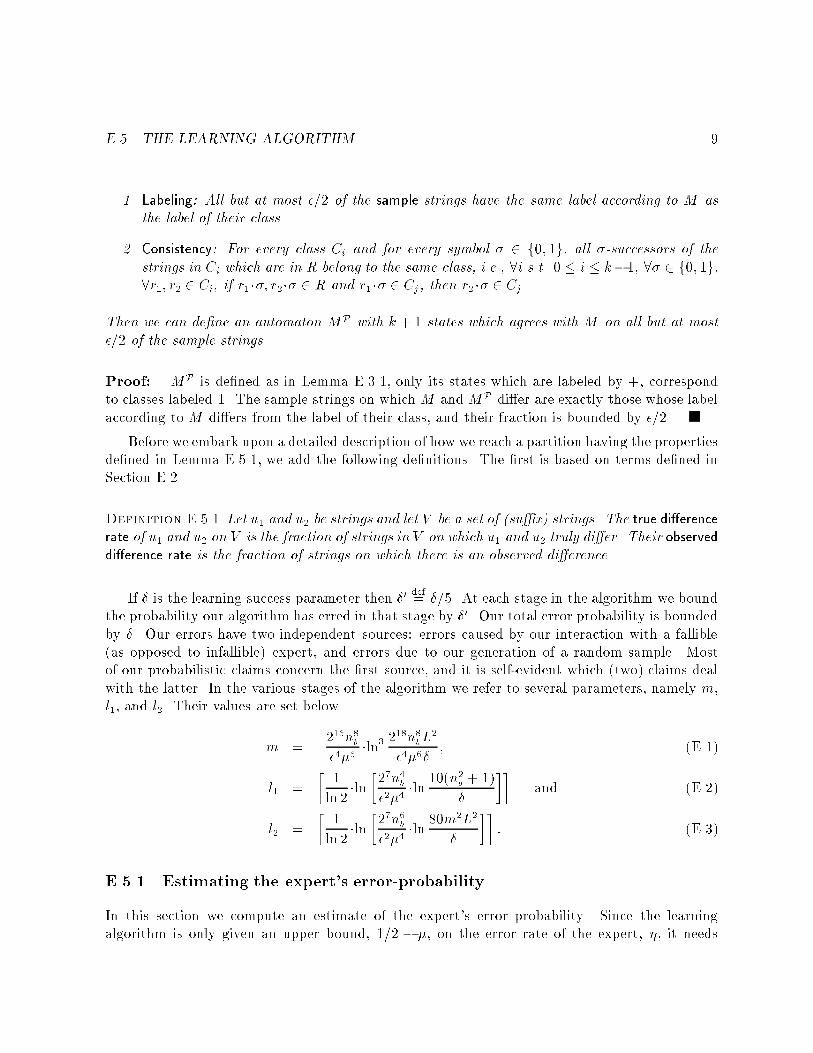
E.5. THE LEARNING ALGORITHM 91. Labeling: All but at most �=2 of the sample strings have the same label according to M asthe label of their class.2. Consistency: For every class Ci and for every symbol � 2 f0; 1g, all �-successors of thestrings in Ci which are in R belong to the same class, i.e., 8i s.t. 0 � i � k�1, 8� 2 f0; 1g,8r1; r2 2 Ci, if r1��; r2�� 2 R and r1 �� 2 Cj, then r2 �� 2 Cj.Then we can de�ne an automaton MP with k + 1 states which agrees with M on all but at most�=2 of the sample strings.Proof: MP is de�ned as in Lemma E.3.1, only its states which are labeled by +, correspondto classes labeled 1. The sample strings on which M and MP di�er are exactly those whose labelaccording to M di�ers from the label of their class, and their fraction is bounded by �=2.Before we embark upon a detailed description of how we reach a partition having the propertiesde�ned in Lemma E.5.1, we add the following de�nitions. The �rst is based on terms de�ned inSection E.2.Definition E.5.1 Let u1 and u2 be strings and let V be a set of (su�x) strings. The true di�erencerate of u1 and u2 on V is the fraction of strings in V on which u1 and u2 truly di�er. Their observeddi�erence rate is the fraction of strings on which there is an observed di�erence.If � is the learning success parameter then �0 def= �=5. At each stage in the algorithm we boundthe probability our algorithm has erred in that stage by �0. Our total error probability is boundedby �. Our errors have two independent sources: errors caused by our interaction with a fallible(as opposed to infallible) expert, and errors due to our generation of a random sample. Mostof our probabilistic claims concern the �rst source, and it is self-evident which (two) claims dealwith the latter. In the various stages of the algorithm we refer to several parameters, namely m,l1, and l2. Their values are set below.m = 216n8b�4�6 �ln3 218n8bL2�4�6� ; (E.1)l1 = � 1ln 2 �ln �27n4b�2�4 �ln 10(n2b + 1)� �� and (E.2)l2 = � 1ln 2 �ln �27n6b�2�4 �ln 80m2L2� �� : (E.3)E.5.1 Estimating the expert's error-probabilityIn this section we compute an estimate of the expert's error probability. Since the learningalgorithm is only given an upper bound, 1=2 � �, on the error rate of the expert, �, it needs

10 APPENDIX E. LEARNING FALLIBLE DETERMINISTIC FINITE AUTOMATAto compute a more exact approximation of �. This approximation is used in later stages of thealgorithm.The basic idea is the following. If two strings reach the same state in M , then any observeddi�erence in their behavior on any set of su�xes is due only to erroneous answers given by theexpert. If two strings reach di�erent states then the observed di�erence in their behavior is due tothe expert's errors and any di�erences in their correct behavior on those su�xes. We show thatfor every pair of strings, and for any set of su�xes V , if both strings reach the same state thentheir expected observed di�erence rate on V is a simple function of the expert's error probability,namely 2�(1� �), and if they reach di�erent states, it is bounded below by this function. Sincethere are at most nb states, given more than nb strings, at least two must reach the same state.Using the fact that the errors are independently distributed, we estimate the expert's errorprobability by looking at the minimum observed di�erence rate between all pairs of strings (amongthose chosen) on a large set of su�xes. We assume that the pair of strings which gives the minimalvalue reach the same state, and calculate the error probability that would generate such anobserved di�erence rate. The above is described precisely in Procedure Estimate-Error appearingin Figure E.2. Procedure Estimate-Error()let W = fw1; :::; wnb+1g be any (arbitrary) set of nb + 1 stringslet V1 be all strings of length l1 over f0; 1gquery the expert on all strings in W �V1for each pair wi 6= wj in W , compute their observed di�erence rate on V1:let �ij jfv j v 2 V1; E(wi �v) 6= E(wj �v))gj=jV1jlet � = mini;j�ijif � > 1=2 then halt and output errorlet ~� be the solution to � = 2~�(1� ~�) such that ~� � 1=2Figure E.2: Procedure Estimate-ErrorIn the following lemma we claim that with high probability � is a good estimate of 2�(1� �)and ~� is a good estimate of �.Lemma E.5.2 Let � = q122�l1 ln 2(nb + 1)2=�0. Then1. Pr[j�� 2�(1� �)j > �] < �0.2. If j�� 2�(1� �)j � � then j~� � �j � �=(2�).In order to prove Lemma E.5.2 we need the following two observations.

E.5. THE LEARNING ALGORITHM 11Observation E.5.1 For any given pair of di�erent strings u1 and u2, and for any given (su�x)string v:1. If M(u1 �v) =M(u2 �v), then Pr[E(u1 �v) 6= E(u1 �v)] = 2�(1� �).2. If M(u1 �v) 6=M(u2 �v), then Pr[E(u1 �v) 6= E(u1 �v)] = (1� �)2 + �2.Hence, if V is any given set of (su�x) strings, and the fraction of strings in V on which u1 andu2 truly di�er is �, then their expected observed di�erence rate on V is(1� �)�[2�(1� �)] + � �[(1� �)2+ �2]= 2�(1� �) + �(1� 2�)2:Observation E.5.2 If u1 and u2 are two di�erent strings, and V is a set of (su�x) strings all ofthe same length, then for every two su�xes vi; vj 2 V , for k and l 2 f1; 2g, uk �vi 6= ul �vj unlessboth k = l and vi = vj. Based on the above and the independence of the noise, for any vi 2 V , theevent that E(u1 �vi) 6= E(u2�vi) is independent of the event that E(u1�vj) 6= E(u2�vj), for all j 6= i.Proof of Lemma E.5.2: 1st Claim: According to Observation E.5.1, for any pair of (di�erent)strings wi and wj in W , if wi and wj reach the same state in M , then for every string v in V1, theprobability that E(wi �v) di�ers from E(wj �v) is 2�(1� �). Thus, according to Inequality 1 andObservation E.5.2 Pr[�ij � 2�(1� �) > �] < e�2�2jV1j (E.4)= e�2�l1 ln 2(nb+1)2�0 jV1j (E.5)= �02(nb + 1)2 : (E.6)Similarly Pr[2�(1� �)��ij > �] < �02(nb + 1)2 : (E.7)If wi; wj reach di�erent states, then for each su�x string v in V the probability that a di�erenceis observed between wi and wj on v is at least 2�(1 � �). Thus Pr[2�(1 � �) � �ij > �] <�0=2(nb + 1)2.We now bound separately the probability that � is an overestimate of 2�(1 � �), and theprobability that it is an underestimate of 2�(1��). What is the probability that � > 2�(1��)+�?Because � was set to be the minimum value of all �ijs, this event occurs only if for all i; j,

12 APPENDIX E. LEARNING FALLIBLE DETERMINISTIC FINITE AUTOMATA�ij > 2�(1� �) + �. Since (nb + 1) � n + 1, there are at least two strings wk and wl that reachthe same state in M and hencePr[�� 2�(1� �) > �] � Pr[�kl � 2�(1� �) > �] (E.8)< �02(nb + 1)2 < �02 : (E.9)In order to underestimate 2�(1� �), it su�ces that for one pair of strings the observed di�erencerate is too small. Since there are less than (nb + 1)2 such pairs,Pr[2�(1� �)�� > �] = Pr[9i; j s.t. 2�(1� �)��ij > �] (E.10)< (nb + 1)2 � �02(nb + 1)2 = �02 ; (E.11)and we have proved the �rst claim.2nd Claim: Assume in contradiction that j~� � �j > �=(2�). If ~� > � + �=(2�) then since ~� wasde�ned to be at most 1=2 and 2~�(1� ~�) is an increasing function in the range between 0 and 1=2,� = 2~�(1� ~�) (E.12)> 2(� + �2�)(1� � � �2�) (E.13)= 2�(1� �) + (1� 2�)�� � �22 2b : (E.14)Since � � 1=2� � we get that � > 2�(1� �) + 2�� �22 2b : (E.15)It is easily veri�ed by substituting the value of l1 in the de�nition of � that � < 2 2b and thus� > 2�(1� �) + � contradicting the assumption in the statement of the lemma.If ~� < � � �=(2�) then � = 2~�(1� ~�) (E.16)< 2(�� �2�)(1� � + �2�) (E.17)= 2�(1� �)� (1� 2�)�� � �22 2b (E.18)� 2�(1� �)� 2�� �22 2b (E.19)< 2�(1� �)� �; (E.20)

E.5. THE LEARNING ALGORITHM 13which again contradicts the assumption.In the following stages of our exposition we assume that in fact � estimates 2�(1� �) withinan additive factor of �, and that ~� estimates � within an additive factor of �=(2�). The probabilitythat this is not true is taken into account in the �nal analysis.E.5.2 Initial partitioning by subsequent behaviorIn the second stage of the algorithm, described in this subsection, we make our �rst step towardsreaching a partition which has the properties de�ned in Lemma E.5.1. By the end of this stagewe are able to de�ne (with high probability) an initial consistent partition Pint of a set of samplestrings and their pre�xes into at most n classes. Each class might include strings which reachdi�erent states in the target automaton M , but strings which reach the same state are notseparated into di�erent classes. We show that Pint has an additional property which is used inthe next stage of the algorithm when the partition is further re�ned.In the partitioning algorithm for the error-free case (described in Section E.3), the set ofsample strings and their pre�xes, R, is �rst partitioned according to the labels of the strings (theirbehavior on the empty su�x). If all strings have the same label then we have a consistent partitioncomposed of a single class. Otherwise, starting from a partition composed of two classes (a `1'class and a `0' class), we try and reach consistency by further re�ning the partition. Wheneveran inconsistency is detected, i.e., there are two strings ri and rj in R which belong to the sameclass, but there exists a symbol � such that ri�� and rj�� di�er on some su�x s and hence belongto di�erent classes, then we have evidence that ri and rj should belong to di�erent classes. Byadding the su�x � �s to S and querying all strings in R�f� �sg to �ll in the new column in theObservation Table T , we automatically re�ne the partition.As noted in Section E.3, the di�erence in behavior between ri and rj on � �s is evidence thatthe two strings reach di�erent states in M , and thus in this process we never separate stringswhich reach the same state into di�erent classes (though strings which reach di�erent states mightbelong to the same class). In the presence of errors however, a di�erence in the observed behaviorbetween two strings on a speci�c su�x, and in particular on the empty su�x (their observedlabels), does not necessarily mean that they reach di�erent states. Hence we must �nd a di�erentprocedure to di�erentiate between strings that reach di�erent states, and then show how to usethis procedure in our quest for a consistent partition.In the previous section we observed (Observation E.5.1), that for any pair of strings and forany set of su�xes V , if both strings reach the same state in M then their expected observeddi�erence rate on V is 2�(1� �), and if they reach di�erent states, it is bounded below by thisvalue. The larger the true di�erence rate between the strings on the set of su�xes is, the larger theexpected observed di�erence is. Thus, since we have a good estimate, �, of 2�(1��), if the set ofsu�xes, V , is large enough, then with high probability we are able to di�erentiate between stringswhich reach states in M whose true di�erence rate on V is substantial. This idea is applied in themost basic building block of our algorithm, described in Function Strings-Test (Figure E.6). This

14 APPENDIX E. LEARNING FALLIBLE DETERMINISTIC FINITE AUTOMATAfunction is given as input two strings, and it returns di�erent if there is a substantial observeddi�erence rate between the two strings on a prede�ned set of equal length strings V2, and similarotherwise.As a consequence, given a set of strings U , we can de�ne an undirected graph G(U), calleda similarity graph. The nodes of G(U) are the strings in U , and there is an edge between everypair of nodes (strings) for which Function Strings-Test returns similar. We show that G(U) hasthe following properties (with high probability):1. Strings in U that reach the same state in M are in the same connected component in G(U).2. For each connected component � in G(U), the fraction of strings v in V2 for which thereexist two strings u and u0 which belong to � but for which M(u�v) 6=M(u0 �v), is small.We refer to the these properties as the �rst and the second properties of similarity graphs . Givena similarity graph G(U) having these properties, and a new string u =2 U , we can add u to thegraph and put an edge between u and all strings u0 2 U such that Strings-Test(u; u0) = similar. Weshow that with high probability the resulting graph G(U[fug) has both properties of similaritygraphs. We next discuss the type of Observation Table constructed in this stage, and describehow similarity graphs are used in its construction.In the error-free case, the algorithm (Procedure Partition-Sample) constructs a data structurein the form of an Observation Table T . In this stage we construct (in Procedure Partition-Erroneous-Sample { Figure E.3) a similar table structure ~T . As in the error-free case, the rowsof the table are labeled by the pre�x closed set R of all sample strings and their pre�xes, and thecolumns are labeled by a su�x closed set of strings S. Initially S includes only the empty stringe, and in the course of the construction we add additional strings. The di�erence between T and~T is that the entrees of T are +=minus valued, where for r 2 R and s 2 S, T (r; s) =M(r�s), whilethe entrees in ~T are names of connected components in the current similarity graph G(R�S). Theentry T (r; s) is the name of the connected component which r �s belongs to in G(R�S), denotedby �G(R�S)(r �s). Equivalently to the error-free case, if row(r) is the row in ~T labeled by r, then,at each stage of the construction, we can de�ne a partition P of R into classes in the followingmanner: two strings r1; r2 2 R belong to the same class in P i� row(r1) = row(r2). ~T and thecorresponding partition P are consistent, i� , for every r1 and r2 in R, and for every � 2 f0; 1g,if row(r1) = row(r2) and both r1 �� and r2 �� are in R, then row(r1��) equals row(r2��).Thus, in order to achieve a consistent partition, we begin by calling Procedure Intialize-Graph(Figure E.4) which constructs the graph G(R). This procedure simply starts with a similaritygraph G(fr1g) consisting of a single node r1 2 R, and adds all other strings in R to the graphby calling Procedure Update-Graph (Figure E.5) on each new string. For every r 2 R we let~T (r; e) = �G(R)(r). At this stage we have a similarity graph which is de�ned on R, but it shall beextended to be de�ned on the growing superset of R, namely R�S.Iteratively, and until the table is consistent, we do the following. If there exist two strings riand rj in R and a symbol � 2 f0; 1g such that row(ri) = row(rj), both ri�� and rj�� are in R, and

E.5. THE LEARNING ALGORITHM 15there exists a su�x s in S such that T (ri ��; s) 6= T (rj ��; s), then we add � �s to S and �ll in thenew column in ~T by determining the connected component in the similarity graph of every stringin R�f� �sg. If a string u in R�f� �sg was in R�S before � �s was added to S, then its connectedcomponent is known. Otherwise, we add u to the graph and simply put an edge between u andevery other node u0 in the graph such that Strings-Test(u; u0) = similar. This is done by callingProcedure Update-Graph on u. If u adds a new (single node) connected component to the graph,or if it is added to a single existing connected component, then we just �ll in the new entry withthe name of this component. If it causes several di�erent connected components in the graph tobe merged into one connected component, then we need to update ~T , so that all appearances ofthe old components are changed into the new one.If strings that reach the same state in M always belong to the same connected component,then the number of times components are merged is at most n, and the total number of columnsin ~T is at most n2. If at any stage the number of classes in the partition de�ned according to ~Tis larger than nb, or the number of columns in ~T exceeds n2b , then we know we have erred and wehalt. Assuming that Function Strings-Test always returns similar when called on pairs of stringsthat reach the same state in M , strings that reach the same state in M always belong to the sameconnected component, and the similarity graphs de�ned by the algorithm always have the �rstproperty of similarity graphs. However, pairs of strings for which Strings-Test returns di�erentsince the observed di�erence rates between the two strings on the set of su�xes V2 is substantial,might also belong to the same connected component due to merging of components. Nonetheless,we show that these mergings of components do not greatly a�ect the second property of similaritygraphs.For ease of the analysis, we de�ne�max def= (1� 2�)�224s2�l2+1(2n2b ln 2 + ln 4N2�0 ) + 2�35 ; (E.21)where � is de�ned in Lemma E.5.2.Lemma E.5.3 Procedure Partition-Erroneous-Sample always terminates, and with probability atleast 1��0, the partition Pint de�ned according to ~T upon termination, has the following properties:1. Pint is consistent (as de�ned in Lemma E.5.1).2. Strings that reach the same state in M belong to the same class in Pint;3. For each class C in Pint, the fraction of su�xes v in V2 on which there exist any two stringsin C that truly di�er on v is at most n��max (where �max is de�ned in Equation E.21).We start by proving a simple claim regarding the correctness of Strings-Test. Let us �rstde�ne what we mean when we say that the function is correct.

16 APPENDIX E. LEARNING FALLIBLE DETERMINISTIC FINITE AUTOMATAProcedure Partition-Erroneous-Sample()Initialization:let R = fr1; r2; : : : ; rNg be the set of all pre�xes of m sample stringsgenerated according to DLS fegcall Initialize-Graph() to construct G(R)�ll in the �rst column of ~T according to G(R):for every r 2 R, ~T (r; e) �G(R)(r)if the number of connected components in G(R) is larger than nb thenhalt and output error.while table is not consistent:8ri; rj 2 R s.t. 8s 2 S T (ri; s) = T (rj; s)if 9� 2 f0; 1g s.t. [ri��; rj �� 2 R and 9s 2 S, s.t. T (ri ��; s) 6= T (rj ��; s)] then doS S [ f� �sgfor every r 2 Rcall Update-Graph(r�� �s) and let G be the current similarity graphif any connected components were merged thenupdate respective entries in ~T~T (r; � �s) �G(r�� �s)if the number of classes in the partition de�ned according to ~Tis larger than nb; or if jSj > n2b thenhalt and output errorf else table is consistent gFigure E.3: Procedure Partition-Erroneous-Sample (Initial Partition)Procedure Initialize-Graph()initialize the similarity graph to be the single node graph G(fr1g)U fr1g (U is the set of strings the similarity graph is de�ned on)for i = 2 to N docall Update-Graph(ri) to add ri to similarity graphU U [ frigFigure E.4: Function Initialize-Graph

E.5. THE LEARNING ALGORITHM 17Procedure Update-Graph(u)if u =2 U then dosim(u) fu0 j u0 2 U; Strings-Test(u,u0) = similar gadd u to similarity graph andput an edge between u and every u0 2 sim(u)U U [ fugf else u is already in the similarity graph gFigure E.5: Procedure Update-GraphFunction Strings-Test(u1; u2)let V2 be the set of all strings of length l2 (over f0; 1g)let �1 q122�l2(2n2b ln 2 + ln 4N2�0 ) + �query the expert on all strings (not previously queried) infu1g�V2 and fu2g�V2let �u1;u2 jfv j v 2 V2; E(u1�v) 6= E(u2�v)gj=jV2jif �u1;u2 > �+ �1 then return di�erentelse return similarFigure E.6: Function Strings-Test

18 APPENDIX E. LEARNING FALLIBLE DETERMINISTIC FINITE AUTOMATAWe say that Strings-Test is correct with respect to a pair of strings u1 and u2 it is called on if thefollowing holds:1. If u1 and u2 reach the same state in M , then Strings-Test(u1; u2) returns similar;2. If u1 and u2 reach di�erent states inM and the fraction of su�xes in V2 on which they trulydi�er is larger than �max then Strings-Test(u1; u2) returns di�erent;Otherwise it is incorrect. If u1 and u2 reach di�erent states in M and the fraction of su�xes inV2 on which they truly di�er is at most �max then the function is correct both if it returns similarand if it returns di�erent.Lemma E.5.4 For any given pair of strings u1 and u2, the probability Strings-Test is correct withrespect to u1 and u2 is at least 1� �0=(4N222n2b).Proof: If u1 and u2 reach the same state in M , then as observed in Observation E.5.1, for everystring v in V2, the probability that E(u1 �v) di�ers from E(u2 �v), is 2�(1� �). Recall that � isthe estimate of 2�(1� �), and according to our assumption � � 2�(1� �)� �. Thus based onInequality 1 and Observation E.5.2Pr[Strings-Test(u1; u2) = di�erent]= Pr[�u1;u2 > �+ �1] (E.22)� Pr[�u1;u2 � 2�(1� �) > �1 � �] (E.23)< e�2(�1��)2jV2j (E.24)= �0=(4N222n2b); (E.25)and hence with probability at least 1� �0=(4N222n2b), Strings-Test(u1; u2) returns similar;If u1 and u2 reach di�erent states in M and the fraction of su�xes on which they truly di�erin V2 is greater than �max, then according to Observation E.5.1, the expected observed di�erencerate between u1 and u2 on V2 is greater than 2�(1� �) + �max(1� 2�)2. ThereforePr[Strings-Test(u1; u2) = similar]= Pr[�u1;u2 � �+ �1] (E.26)� Pr[E(�u1;u2)��u1;u2 > �max(1� 2�)2 � �1 � �] (E.27)< �0=(4N222n2b); (E.28)and hence with probability at least 1� �0=(4N222n2b), Strings-Test(u1; u2) returns di�erent.Proof of Lemma E.5.3: Procedure Partition-Erroneous-Sample terminates either when thetable is consistent, or when the number of classes in the partition de�ned by ~T is larger than nb,or when the number of su�xes in S is larger than n2b . Since each time inconsistency is detected

E.5. THE LEARNING ALGORITHM 19we add a new su�x to S, if the procedure does not terminate due to the �rst reason mentionedabove, it must terminate due to the third reason, and hence it always terminates.In order to prove that with probability at least 1 � �0, Pint has the properties de�ned in thelemma, we show that if Function Strings-Test is correct with respect to every pair of strings it iscalled on, then Pintmust have these properties. We would have liked to bound the probability thatStrings-Test is correct with respect to every pair of strings it is called on, simply by the numberof pairs of strings it is called on, times the bound given in Lemma E.5.4 on the probability it errson one pair. However, since the pairs of strings Strings-Test is called on are not all chosen priorto receiving any of the experts labels, but rather are chosen dynamically, where the choice of anew pair depends on previous answers given by the expert, we may not use this simple bound.Instead, we need to consider all possible pairs of strings Strings-Test may be called on, given ourchoice of R.Let S be the set of all strings over f0; 1g of length at most n2b . By de�nition of ProcedurePartition-Erroneous-Sample, the size of S does not exceed n2b . The initial su�x put in S, e, is oflength 0, and every su�x added to S is at most one symbol longer than the longest su�x alreadyin S. The above implies that all strings in S have length at most n2b . Hence, S is always a subsetof S. Let D(R) def= fR�Sg�fR�Sg. Then the set of pairs of strings which Strings-Test is called onis always a subset of D(R). Since the size of D(R) is at most (N �2�2n2b)2, if we apply Lemma E.5.4to every pair of strings in D(R), then we get that the probability that Strings-Test is correct onall pairs in D(R), (which are all possible pairs it may be called on given R), is at least 1� �0.From now on we assume that Strings-Test is correct with respect to all pairs of strings it iscalled on. We refer to this assumption in the next steps of this proof as the correctness assumption.Based on the correctness assumption we now prove that Pint has all three properties de�ned inthe lemma.2nd Property: Based on the correctness assumption, and the construction of the similaritygraphs, strings which reach the same state always belong to the same connected component.Since two strings ri and rj in R belong to di�erent classes in Pint only if for some su�x s in S,ri �s and rj �s belong to di�erent components (and thus reach di�erent states), then the followingmust also be true. At any stage in the procedure, strings in R that reach the same state, belongto the same class (in the partition de�ne according to ~T at that stage). Thus, in particular, Pinthas the second property de�ned in the lemma.1st Property: In order to prove that Pint is consistent we must show that under the correctnessassumption, Procedure Partition-Erroneous-Sample does not terminate with an error message,which means that it must terminate \naturally" when ~T , and hence Pint, are consistent. We havejust shown in the previous paragraph that the number of classes in the partition de�ned in anystage of the procedure, is at most n, which is bounded by nb. Hence the procedure does not haltdue to the number of classes being larger than nb. It remains to show that the number of su�xesadded to S is no larger than n2b .Each time connected components are merged, the number of components decreases by at least

20 APPENDIX E. LEARNING FALLIBLE DETERMINISTIC FINITE AUTOMATA1. Since the number of components at any stage can be no larger than n, components are mergedat most n � 1 times. (If all strings belong to the same component then we necessarily havea consistent partition). Every time a su�x is added and no components are merged, then thepartition is re�ned, and the number of classes grows by at least 1. Hence, between every twomerges of components we can add at most n� 1 su�xes to S, and the total number of su�xes inS is bounded by n2b .3rd Property: We prove that this property holds after every call to Update-Graph, and for eachset of strings that belong to the same connected component at that stage. Since strings in Rwhich belong to the same class belong to the same connected component, the claim follows.For each connected component � we de�ne the following undirected graph G�M . The nodes inG�M are states in M reached by strings belonging to �. We put an edge between two states q andq0 i� there is an edge in � between some pair of strings u and u0 such that u reaches q in M andu0 reaches q0. Since � is a connected component, G�M must be connected as well.Given one such graph G�M , we look at any arbitrary spanning tree of the graph. For each edge(q1; q2) in the tree, let D(q1; q2) be the subset of strings in V2 on which q1 and q2 truly di�er.Under the correctness assumption, jD(q1; q2)j � �max�jV2j. Let u and u0 be two strings in � whichreach q and q0, respectively. Let q = q1; q2; : : : ; ql = q0, be a path in the tree between q and q0.Then all the su�xes in V2 on which u and u0 truly di�er belong to Sl�1i=1D(qi; qi+1). Hence, allthe su�xes v in V2 such that there exist any two strings in � that truly di�er on v must belongto the union of D(qi; qj) over all edges (qi; qj) in the spanning tree of G�M . Since the number ofnodes in G�M is at most n, so are the number of edges in any spanning tree of the graph, and theclaim follows.We assume from now until the �nal analysis that Pint has the properties de�ned in LemmaE.5.3.Two ExamplesIn this subsection we begin to describe two example runs of our algorithm. We complete thisdescription in Section E.7 after we present the next and �nal stage of the algorithm.q 0 q 1

0/1

0/1Figure E.7: First example target automaton. q1 is the single accepting state.

E.5. THE LEARNING ALGORITHM 21In the �rst example, the target automaton is a two state automaton over the alphabet f0; 1g,which accepts all strings of odd length (and rejects all strings of even length). It is depicted inFigure E.7. We now describe what happens in the initial partitioning. For every pair of strings riand rj in R such that ri reaches q0 and rj reaches q1, ri and rj di�er on all strings in V2. Hence,with high probability, all strings in R that reach q0 initially are in the same connected componentin G(R), and all strings that reach q1 are in a di�erent connected component. After �lling in the�rst column in ~T labeled by e, we already have a consistent partition into two classes C0 and C1,where all strings in C0 reach q0 and all strings in C1 reach q1. Since the classes in this partitionexactly correspond to the states of the target automaton, there exists a labeling of the classesthat has the labeling property de�ned in Lemma E.5.1. However, in Section E.7 we describe howwe �rst further re�ne the partition before labeling the classes.q 0

q 1

q 2

q 3

q 4

0/1

0/1

0

0

0

11

1

Figure E.8: Second example target automaton. q3 is the single accepting state.In the second example, the target automaton is a �ve state automaton over the alphabetf0; 1g, which accepts all strings of length 2 modulo 3 which end either with the symbols 00 orwith the symbols 11 (and rejects all other strings). It is depicted in Figure E.8.Assume that the length of l2 is 0 modulo 3 (the other two cases are very similar). Then forevery pair of strings ri and rj in R such that ri reaches one of q0, q1 or q2 and rj reaches either q3or q4, ri and rj truly di�er on exactly half of the strings in V2 (all those that end either with a 00or with a 11). For every pair of strings ri and rj such that ri reaches one of q0, q1 or q2, and rjreaches a di�erent state among these three states, ri and rj truly behave the same on all stringsin V2. The same is true for every pair of strings that reach either q3 or q4. Hence, with highprobability, all strings in R that reach one of q0, q1 or q2 are initially in one connected componentin G(R), and all strings that reach q3 or q4 are in a di�erent connected component.

22 APPENDIX E. LEARNING FALLIBLE DETERMINISTIC FINITE AUTOMATAAfter �lling in the �rst column in ~T labeled by e with the names of these two components, weshall observe the following inconsistency. If ri is a string that reaches q0, and rj is a string thatreaches either q1 or q2, and if for � = 0=1, both ri��, and rj �� are in R, then ri�� and rj �� are indi�erent connected components (since ri �� reaches either q1 or q2, and rj �� reaches either q3 orq4). After resolving this inconsistency by adding � to S, the table is consistent, and we have threeclasses. Let us denote these classes by C0, C1=2 and C3=4, where strings in C0 reach q0, stringsin C1=2 reach either q1 or q2, and strings in C3=4 reach either q3 or q4. It is clear that there is nolabeling of these classes that has the labeling property de�ned in Lemma E.5.1, unless there areeither very few strings in R that reach q3, or very few that reach q4. In Section E.7 we show howthis partition is further re�ned, and how the new classes are labeled.E.5.3 Final partitioning by correctionWe reach this stage with an initial partition Pint that has with high probability the propertiesde�ned in Lemma E.5.3. In this section we continue re�ning Pint. The �nal partition, Pfnl,remains consistent. We then label the classes in Pfnl, so that with high probability the labeledpartition has the labeling property de�ned in Lemma E.5.1. Namely, for most sample strings, thelabel of their class is their correct label. We give an upper bound on the number of classes inPfnl, so that in Section E.6 we can use an Occam's Razor type of argument in order to prove thatwith high probability the hypothesis automaton de�ned based on Pfnl is an �-good hypothesis.The resulting automaton might be much larger than the minimal equivalent automaton and so weapply an algorithm for minimizing DFA's [Huf54, Moo56, Hop71] and �nd the smallest equivalentautomaton.The �nal partition is de�ned in the following simple manner. For any given string r 2 R suchthat jrj � l2, let r = rp�rs where jrsj = l2. Let the pre�x class of r, denoted by Cp(r) be the classrp belongs to in Pint. ThenPfnl def= f fr j jrj � l2; Cp(r) = C; rs = sg j C 2 Pint; jsj = l2g[ ffrg j jrj < l2g : (E.29)Pfnl is a re�nement of Pint since all strings that have the same pre�x class and the same su�x(of length l2) must belong to the same class in the initial partition. For each class C 2 Pint, andfor every string s of length l2, let (C; s) denote the class in Pfnl which consists of all strings inR whose pre�x class is C, and whose su�x of length l2 is s. There are at most nb �2l2 classes ofthis kind, and at most 2l2 singleton classes each consisting of a single string of length less than l2.The size of the �nal partition is hence at most (nb + 1)2l2, and thus grows only logarithmicallywith the sample size m. We later show that since the initial partition is consistent, so is this �nalpartition.The classes in Pfnl are labeled by calling Procedure Label-Classes (Figure E.9). For each class(C; s) the procedure labels the class by the majority observed label of the strings in C�fsg. If allstrings in C truly behave the same on the su�x s, and if C is of substantial size, then with high

E.5. THE LEARNING ALGORITHM 23probability the majority observed label is the true label of all strings in the class (C; s) (which isequivalent to fC�fsgg\R). In this case we say that (C; s) is a good class. Based on the assumptionthat Pint has the third property de�ned in Lemma E.5.3, we show that the fraction of samplestrings whose correct label di�ers from the label of their class, is small, and hence Pfnl has thelabeling property de�ned in Lemma E.5.1. The singleton classes are all labeled by a default value�, since we do not have a reliable way of determining their correct labels. This is an arbitrarychoice and any other labeling of these classes would not alter our analysis. In particular, there aresome special cases where a di�erent labeling would give a better bound on the number of statesin the hypothesis automaton. We return to this issue at the end of this subsection.The initial partition thus serves two purposes. It is used as a basis for the �nal partition, andit is used to compute the correct labels of most sample strings.Procedure Label-Classes()for each class (C; s) 2 Pfnllet the label of (C; s) be maj(E(r�s) j r 2 C).for each class frig 2 Pfnl (where jrij < l2)let the label of frig be 0.Figure E.9: Procedure Label-ClassesLemma E.5.5 1. With probability at least 1�2�0, The fraction of sample strings whose correctlabel di�ers from the label computed for their class by Procedure Label-Classes is at most�=2.2. Pfnl is always consistent, and jPfnlj � (nb + 1)2l2.Our main e�orts are directed towards proving the �rst claim of Lemma E.5.5. In order to dothis we need to bound the fraction of sample strings for which the label computed by Label-Classesfor their class is incorrect with non-negligible probability.We �rst formally de�ne the notions of good and bad classes mentioned previously.Definition E.5.2 We say that a class (C; s) 2 Pfnl is good if all strings in C truly behave thesame on s. Otherwise it is bad.We know (Lemma E.5.3) that with high probability, for every class C in Pint, the fractionof su�xes s for which (C; s) is bad, is small. We would like to prove that with high probabilitythe sample chosen is such that most sample strings of length at least l2 belong to good classes in

24 APPENDIX E. LEARNING FALLIBLE DETERMINISTIC FINITE AUTOMATAPfnl. To do so we prove that with high probability no string of length l2 is a su�x of too large afraction of the sample strings. Assuming this is the case, then in particular all strings s for whichthere exists a class C 2 Pint, such that (C; s) is bad can not be su�xes of too large a fraction ofthe sample strings, and only this small fraction of the sample strings belong to bad classes.Lemma E.5.6 With probability at least 1� �0, there is no string of length l2 which is a su�x ofmore than a fraction of 2�l2+1 of the sample strings.Proof: Since the sample strings are uniformly distributed, for every given su�x of length l2, theexpected fraction of sample strings having that su�x is 2�l2 . Applying Inequality 2, we get thatfor every given su�x of length l2, the probability that there are more than 2m�2�l2 strings withthat su�x (i.e., twice the expected number) is less than e� 13 2�l2m. The probability this occurs forany su�x of length l2 is less than 2l2e� 132�l2m, which is less than �0 since m > 3�2l2 ln(2l2=�0).There are two more types of classes in the �nal partition for which we cannot claim Label-Classes is reliable in their labeling (even though they are good) and which we deal with in theproof of Lemma E.5.5: the singleton classes and the classes (C; s) for which jCj is small. In orderto prove that with high probability Procedure Label-Classes correctly labels all classes (C; s) whichare good and for which jCj is not too small, we need the following simple claim.Lemma E.5.7 Let B be any set of strings which have the same correct label ` 2 f0; 1g, and let0 < �00 < 1. If jBj � 12��2(ln 1=�00), then with probability at least 1 � �00, the majority observedlabel of the strings in B is `.Proof: Since the expected value of the observed majority label is 1� �,Pr[ majority observed label is wrong ] < e�2(12��)2 jBj � e�2�2jBj � �00:We are now ready to prove Lemma E.5.5.Proof of Lemma E.5.5:1st Claim: As mentioned previously, there are three kinds of sample strings for which the labelof their class in Pfnl might di�er from their correct label:1. Strings shorter than l2.2. Strings which belong to bad classes.3. Strings which belong to good class (C; s) but for which the majority value of the observedlabels in C�fsg is incorrect.There are at most 2l2 � (�=8) �m of the �rst kind.

E.5. THE LEARNING ALGORITHM 25We next turn to the second kind of mislabeled strings. Based on our assumption that Pint hasthe third property de�ned in Lemma E.5.3, we know that for each class C 2 Pint, the fractionof strings s 2 V2, such that (C; s) 2 Pfnl is bad, is at most n ��max (where �max is de�ned inEquation E.21). There are at most n classes in Pint, and hence the fraction of strings s in V2such that there exists any class C 2 Pint for which (C; s) is bad is at most n2 ��max. ApplyingLemma E.5.6, we get that with probability at least 1��0 the fraction of mislabeled sample stringsof the second kind is at most2n2 ��max = 2n2(1� 2�)�224s2�l2+1(2n2b ln 2 + ln 4N2�0 ) + 2�35 : (E.30)Bounding (1� 2�) from below by 2�, and substituting the values of l2 and � in Equation E.30 weget that 2n2 ��max � n2b��2=2� " s �2�426n6b ln 20m2L222� �(2n2b ln 2 + ln 4m2L2�0 )+ 2vuut �2�428n4b ln 10(n2b+1)� � ln 2(nb + 1)2=�0 35< �8 (E.31)It remains to bound the fraction of mislabeled sample strings of the third kind. We show thatwith probability at least 1� �0 there are less than (�=4)m mislabeled sample strings of this kind.It follows that with probability at least 1 � 2�0, the fraction of mislabeled sample strings of anyone of the three types mentioned above is at most �=2.Let (C; s) be a good class, and let jCj � �2, where�2 def= 12��2(nb ln 2 + ln 2l2�0 ): (E.32)Based on Lemma E.5.7, the probability that the majority observed label of the strings in C�fsg isnot their correct (common) label, is less than �0=(2nb2l2). For a given class C 2 Pint, the numberof (nonempty) classes (C; s) is at most 2l2 . The initial partition into classes (which induces apartition into pre�x classes) is not chosen independently from the expert's (correct and incorrect)labels of the strings in R�V2, but is rather de�ned based on the knowledge of these labels. Hence,we must consider all possible pre�x classes of strings in R. We assume that the initial partitionhas the properties de�ned in Lemma E.5.3, and speci�cally that it has the second property de�nedin the lemma, namely that all strings that reach the same state in M belong to the same class inthe initial partition. Since there are at most 2nb subsets of the states in M , and each such subsetX corresponds to a potential class in the initial partition (which includes all strings in R that

26 APPENDIX E. LEARNING FALLIBLE DETERMINISTIC FINITE AUTOMATAreach states in X), there are at most 2nb possible pre�x classes. Therefore, the probability thatfor all possible pre�x classes C of size at least �2, and for all possible su�xes s such that (C; s)is a good class, the majority observed label of the strings in C�fsg is the correct label, is at least1� �0.Therefore, with probability at least 1��0, all mislabeled strings of this (third) kind are stringswhich belong to classes (C; s) such that jCj < �2. For each such C, the number of sample stringswhich belong to (C; s) for any s, is at most �22l2 . There are less than nb such classes, and hencethe number of mislabeled strings of this kind is less thannb�22l2 � 12nb��2 �nb ln 2 + ln( 28n6b�2�4�0 � ln 80m2L2� �� 28n6b�2�4 � ln 80m2L2� (E.33)< 27n8b�2�6 � �ln 29n6b�2�4�0 + ln ln 40m2L2� �� ln 40m2L2� (E.34)< �=4m (E.35)2nd Claim: The bound on the size of Pfnl follows directly from its de�nition. It remains to showthat it is a consistent partition. Let (C; s) be any class in Pfnl where s = s1 : : : sl2 , let � be asymbol in f0; 1g, and let r1 = r1p�s and r2 = r2p�s be two strings which belong to (C; s) such thatboth r1 �� and r2 �� are in R. Since r1 and r2 both have the same su�x of length l2, so do r1 ��and r2��. Since r1 and r2 have the same pre�x class C in Pint (i.e., r1p and r2p belong to the sameclass in Pint), and Pint in consistent, r1�� and r2�� must have the same pre�x class as well (sincer1p�s1 and r2p�s1 must belong to the same class). It follows that r1�� and r2�� belong to the sameclass in Pfnl.In Lemma E.5.5 we give an upper bound on the number of classes in the partition which isconsiderably larger than the number of states in the target automaton. As mentioned previously,we can try and minimize the automaton de�ned based on this partition. If all classes (C; s) aregood and all classes (including the singletons) are correctly labeled, and if we do not need to addthe sink class, then this minimization results in an automaton of size at most n. Though we donot have a general way to avoid errors resulting from the existence of bad classes or of small pre�xclasses, we can sometimes avoid errors when labeling the singleton classes.As we have mentioned in our discussion of Procedure Label-Classes (prior to the analysisabove), our choice of labeling by 0 all singleton classes, is arbitrary, and any other labeling willdo. We next describe a case in which a di�erent labeling is more advantageous.Assume that Pfnl consists only of good classes (C; s) for which jCj � �2. In particular, thismay be the case when Pint exactly corresponds to the target automaton in the sense that notwo strings which belong to the same class in the initial partition reach di�erent states, and for

E.6. PUTTING IT ALL TOGETHER 27each state there exists a string that reaches it. If the target automaton is such that: (1) thereis non-negligible probability of passing each state in a random walk of length L; (2) every twostates either di�er on a non-negligible fraction of strings of length l2, or reach such a pair of states(that di�er on a non-negligible fraction of strings of length l2) on a walk corresponding to somestring s; then with high probability Pfnl has the properties mentioned above. The �rst exampledescribed in Subsection E.5.2 is of this type.Suppose that when labeling the classes (C; s) we notice that for a class C 0 2 Pint, all classes(C; s) which include strings that belong to C 0 are labeled the same. Then we label all singletonclasses which include strings that belong to C 0 with the same label. If the initial partition in factcorresponds to the target automaton, then this labeling is correct with high probability.E.6 Putting it all togetherWe have shown how to achieve with high probability a labeled partition of a given set of samplestrings and their pre�xes that is consistent and for which the fraction of sample strings whoselabel according toM di�ers from the label of their class is at most �=2. We have also shown thatthe number of classes in this partitioning is at most � lnm where � is a polynomial in nb, 1� , L, 1�and ln 1� . Hence, we can apply Lemma E.5.1 and construct a hypothesis automaton with � lnmstates which agrees with M on all but �=2 of the sample strings. Adding up the probabilitiesour algorithm errs in each of its stages and using the following Occam's Razor-like lemma, weprove that with probability at least 1� �, our hypothesis automaton is an �-good hypothesis withrespect to M and DL.Lemma E.6.1 Let � be a polynomial in nb; 1� ; L; 1� ; and ln 1�0 ; and let�0 = max(4� log2 �; ln 1�0 ). Given m � 64�0�2 (ln 64�0�2 )3 strings chosen according to DL, if anautomaton of size at most � lnm disagrees with M on no more than �=2 of the sample strings,then the probability that it is an �-bad hypothesis with respect to M is at most �0.Proof: LetM 0 be an automaton of size at most � lnm which is an �-bad hypothesis with respectto M . Given a random sample of size m labeled according to M , the expected number of stringson which M 0 disagrees with M is at least �m. According to Inequality 1, the probability thatM 0disagrees with M on no more than �2m of the m random strings, is at most e�2(�=2)2m. Since thenumber of automata which are �-bad hypotheses with respect to M is at mostNDFA(� lnm)� 1 < 24� lnm log(� lnm)< 2�0(lnm)2 ;the probability we found such an automaton which disagrees with M on no more than �2 of thesample strings is at most 2�0(lnm)2e� 12 �2m. But for m � 64�0�2 (ln 64�0�2 )3m(lnm)2 � 64�0�2 (ln 64�0�2 )3(ln 64�0�2 + 3 ln ln 64�0�2 )2 (E.36)

28 APPENDIX E. LEARNING FALLIBLE DETERMINISTIC FINITE AUTOMATA� 64�0�2 (ln 64�0�2 )316(ln 64�0�2 )2> 4�0�2 :Thus �0(lnm)2 < 14�2m: (E.37)And so 2�0(lnm)2e� 12 �2m < e� 14 �2m < e�16�0 < �0: (E.38)It is easily veri�ed that the algorithm we have described is polynomial in nb, 1� , L, 1� and ln 1� .Consequently we have proven our main theorem:Theorem E.1 The algorithm described in Section E.5 is a good learning algorithm for fallibleDFA'sE.7 Examples RevisitedWe now return to the example runs presented in Subsection E.5.2 and see how the algorithmcompletes these runs.We start with the �rst example. Remember that following the initial partitioning we have twoclasses - C0 includes the strings in R that reach the state q0 and C1 includes the strings that reachq1. For each class Ci (i 2 f0; 1g), all strings in the classes (Ci; s) (jsj = l2) in Pfnl, and in general,all strings in the sets Ci�fsg have the same correct label since they belong to the same class inPint. Assuming that both C0 and C1 are larger than �2,2 all these classes are labeled correctly.If all singleton classes are labeled 0, then the automaton based on this partition (depictedin Figure E.10) has the following form. It consists of a complete binary tree of depth l2 � 1whose states are all rejecting states, and whose root, e is the starting state of the automaton.All transition from the leaves of this tree are to the states (C0; s) which are all rejecting states.All transition from this layer are to the layer of states (C1; s), which are all accepting states, andwhich traverse back to the �rst layer. The minimized automaton is depicted in Figure E.11.Note that if we use the modi�ed version of Label-Classes as described in the end of Subsec-tion E.5.3 for labeling the singleton classes, then we can label these classes correctly as well. The(minimized) hypothesis automaton which is based on Pfnl is equivalent to the target automaton.2If they are not, this is because the sample is not typical. The probability such an event occurs is taken intoaccount in Lemma E.6.1.

E.7. EXAMPLES REVISITED 29Also note that in this example (when the modi�ed version is not used), the following modi�-cation can be employed as well. Since all strings of a given length reach the same state, and sincethe �rst l2 states do not belong to the strongly connected component of the underlying graph,and hence only the short strings (which we already \gave up" on their correct labeling) reachthem, we can remove the �rst l2 states from the hypothesis. The new starting state is chosen sothat the longer strings reach the states corresponding to their class in the �nal partition, and aretherefore labeled the same by the modi�ed hypothesis as by the original hypothesis. The modi�edhypothesis is then equivalent to the target automaton.(C0 ,s) (C1 ,s)

l 2 - 1

.

.

.

0/1

0/1

0/1

0/1

0

1

_

_

. . .1

λ

11

10

0

0

0

Figure E.10: Hypothesis automaton for the �rst example.l2 q l2+10 qq q

1 -1l2q

0/1

0/1

. . .0/10/1Figure E.11: Hypothesis automaton for the �rst example (minimized version).We now return to the second example. Remember that in this example, strings that belongto the same class in Pint do not necessarily have the same correct label. Speci�cally, part of thestrings in the class C3=4 reach an accepting state (q3) in the target automaton, and part of thestrings reach a rejecting state (q4). Note though, that all strings in this class that end either

30 APPENDIX E. LEARNING FALLIBLE DETERMINISTIC FINITE AUTOMATAwith a 00 or with a 11 reach q4, while all other strings reach q3. Based on our assumption thatthe length of l2 is 0 modulo 3 (as noted previously, the other two cases are very similar), thepre�x class of all strings in C3=4 is C3=4. For every s, jsj = l2 of the form s000 or s011, all stringsin C3=4�fsg have the same correct label 1, and for every s of the form s001 or s010, all stringsin C3=4�fsg have the same correct label 0. Assuming C3=4 is larger than �2, all these classesare labeled correctly. Similarly, if both C0 and C1=2 are larger than �2, then all classes (C0; s),(C1=2; s), and (for every s) are labeled correctly by 0.If all singleton classes are labeled 0, then the automaton based on this partition will havethe form depicted in Figure E.12. Its minimized version is depicted in Figure E.13. In this casethe modi�cation of Label-Classes mentioned in the �rst example cannot help label the singletonclasses correctly. However, equivalently to the �rst example, we can remove the states that donot belong to the strongly connected component and choose the new starting state accordingly.l 2 - 1

(C0 ,s)

(C3/4,s’’00)

(C3/4

(C3/4,s’’01)

(C3/4 ,s’’10)

1_

0

1

.

.

.

0

0

1

1

0/1

0/1

0

1

,s’’11)

0/1

0/1

0/1

0/1

(C1/2,s’0)

(C1/2,s’1)

0_

. . .

1

0

0

0

1

1

λ

Figure E.12: Hypothesis automaton for second example.E.8 ExtensionsAs mentioned in the Introduction, our result can be extended to the following cases:

E.8. EXTENSIONS 31q 0 q 1

q l2-1

q l2

q l2

q l2+2

q l2+3

q l2+4

0/1

0/1

0

0

0

11

10/1 0/1. . .

+1

Figure E.13: Hypothesis automaton for second example (minimized version).1. The expert's errors are not completely independent but rather are distributed only k-wiseindependently for k = O(1).2. The expert's error probability is dependent on the length of the input string.3. The target automaton has more than two possible outputs (the extension to larger inputalphabets is completely straightforward).We �rst describe in short the changes that should be made to the algorithm in each of thecases above and then discuss brie y some other possible extensions.E.8.1 k-wise Independence of the Expert's Error ProbabilityIn this case, the algorithm need not be altered, only the size of the sample and the sizes l1 and l2 ofthe length of the su�xes on which the sample strings behavior is tested need to be changed. Thisis due to the fact that we cannot use Inequality 1 when bounding the error probability in di�erentstages of the algorithm, since Inequality 1 is only valid under the assumption that the randomvariables are independent. Instead, we can use the following inequality that is derived from thehigh moment inequality of which Tchebychev's inequality is a special case. Let X1; X2; ::::XMbe M k-wise independent 0=1 random variables where Pr[Xi = 1] = pi, and 0 < pi < 1. Letp =Pi pi=M .Inequality 3 For 0 < � � 1: Pr[jPMi=1XiM � pj > �] < kkM k2 ��k

32 APPENDIX E. LEARNING FALLIBLE DETERMINISTIC FINITE AUTOMATAIf all pi's are equal then we can get a slightly better bound in which the above expression ismultiplied by p k2 .In order that our claims regarding the upper bounds on the error probabilities in all the stagesof the algorithm remain true, we must enlarge the size of our sample, m, and the size of the setsV1 and V2 on which we test the behavior of the sample strings. It can be shown that the size ofthese sets remains polynomial in the relevant parameters of the problem, and that the size of thehypothesis automaton grows like m� for � < 1. Therefore the learning algorithm remains a goodlearning algorithm for fallible DFA's.E.8.2 The Expert's Error Probability is Dependent on the Length of the InputStringsIn this case we assume that for every length l � 0, the expert errs with probability �l � 1=2�� onstrings of length l. We use the same technique presented in Section E.5.1, for estimating each �l,only now we compute the corresponding estimate, �(l), of 2�l(1� �l), for every l1 � l � L+ l23.This is done by picking a set Wl of nb + 1 strings all of the same length l � l1 and letting �(l)be the outcome of Function Estimate-Error (Figure E.2) when executed on the set Wl (and, asbefore, on the set of all su�xes of length l1). When bounding the error probability of the revisedalgorithm, we must take into account that we want that with high probability all estimates �(l)be approximately correct.The fact that the error probability might di�er for di�erent string lengths must be taken intoaccount in the following places:1. The statements in Observation E.5.1 should now be: For any given pair of di�erent stringsu1 and u2, and for any given (su�x) string v:(a) If M(u1 �v) =M(u2 �v), thenPr[E(u1 �v) 6= E(u1 �v)](1� �juij+jvj)�jujj+jvj + (1� �jujj+jvj)�juij+jvj:(b) If M(u1 �v) 6=M(u2 �v), thenPr[E(u1 �v) 6= E(u1 �v)] = (1� �juij+jvj)(1� �jujj+jvj) + �juij+jvj�jujj+jvj:Hence, if V is a set of (su�x) strings, all of length l, and the fraction of strings in V onwhich u1 and u2 truly di�er is q, then their expected observed di�erence rate on V is�ju1j+l + �ju2j+l � 2�ju1j+l�jtjj+l + q(1� 2�ju1j+l)(1� 2�ju2j+l):3The values of l1 and l2 must be changed accordingly but their usage is the same as in the original version ofthe algorithm

E.8. EXTENSIONS 33In the special case where ju1j = ju2j = l0 we of course get the same result as in the originalversion of Lemma E.5.1, where � is exchanged by �l0+l .Thus there is still a gap between the expected value of the observed di�erence in behaviorin the case where two strings reach the same state and in the case they do not reach thesame state. When exploiting this gap in the process of the initial partitioning (speci�cally inFunction Strings-Test appearing in Figure E.6), we must take into account that the expectedvalue of the observed di�erence rate between two strings depends on their lengths, and usethe correct expression.2. In general, as mentioned in speci�c cases above, the value of almost all parameters (the sizeof the sample m, the lengths, l1 and l2, of the su�x strings on which we test the samplestrings, the value of �1 in Function Strings-Test, etc.) must be revised so that the totalerror probability of the algorithm is bounded by �.E.8.3 Multiple OutputsAssume that the target automaton has more than two possible outputs, and let the outputalphabet be denoted by �. Assume also that the error process is such that for every (newly)queried string u, independently, and with probability �, the expert's answer, E(u), received forthat string, is chosen uniformly from ��fE(u)g. We claim that if we slightly modify some of theparameters of our algorithm, then it remains a good learning algorithm in this case.There are several places in the algorithm and its analysis where the fact that j�j > 2 has tobe taken into account: in Observation E.5.1 which implies slight changes in Procedure Estimate-Error , Lemma E.5.2 and Lemma E.5.4; and in Lemma E.5.7.It is very easy to verify that Lemma E.5.7 remains correct. Actually it su�ces that ProcedureLabel-Classes label the classes according to their most common observed label. For a given set ofstrings which have the same correct label, the probability that the most common observed labelis incorrect decreases very rapidly when j�j increases.Observation E.5.1 is generalized as follows:Observation E.8.1 For any given pair of di�erent strings u1 and u2, and for any given (su�x)string v:1. If M(u1 �v) =M(u2 �v), then Pr[E(u1 �v) 6= E(u1 �v)] = 2�(1� �) + �2(1� 1=(j�j � 1)).2. If M(u1�v) 6=M(u2�v), then Pr[E(u1�v) 6= E(u1�v)] = (1� �)2+2�(1� �)(1� 1=(j�j� 1))+�2(1� (j�j � 2)=(j�j � 1)).It is not hard to verify that if V is any given set of (su�x) strings, and the fraction of strings inV on which u1 and u2 truly di�er is �, then their expected observed di�erence rate on V is2�(1� �) + �2(1� 1=(j�j � 1) + � �(�; j�j); (E.39)

34 APPENDIX E. LEARNING FALLIBLE DETERMINISTIC FINITE AUTOMATAwhere (�; j�j) is at least (1� 2�)2 (for j�j � 2), which was the gap we had when j�j = 2. Giventhis observation, we can slightly modify Procedure Estimate-Error in order to compute a goodestimate, �, of 2�(1� �) + �2(1 � 1=(j�j � 1), and extract from it a good estimate of �. Basedon the gap mentioned above, and using these estimates, we can apply Function Strings-Test, asin the case of j�j = 2, in order to di�erentiate between strings that reach states in M whose truedi�erence rate on V is substantial. In the analysis of the correctness of Strings-Test , described inLemma E.5.4, we need only take into account the change in the de�nition of �.E.8.4 Additional ExtensionsOur main assumption in this work is that the error probability of the expert is �xed. As mentionedin the previous subsection, we can deal with the special case in which the error probability isdependent on the length of the input string. The general problem (in which for every string u theexpert has a (possibly di�erent) error probability �(u)) seems hard. It might be argued that thenatural problem in this case is to learn the corresponding probabilistic concept [KS90]. What wewould like to know is if there are other (reasonable) special cases for which our algorithm can beadapted. For example, can the problem be solved if the error probability of the expert dependson the state reached by the input string?Another generalization of our algorithm is to modify it to work under additional distributionsother than the uniform distribution. It is unreasonable to expect to �nd an algorithm that worksunder any input distribution. For example assume that all the weight of the distribution is onone string, or even that it is equally divided among n strings each reaching a di�erent state. Inthese cases, for each string in the support of the distribution, with probability � it is labeledincorrectly, and we have no way of determining its correct label. However, it may be possible thatour algorithm can be modi�ed to work for other \natural" distributions.4One additional point is the question of the practicality of the algorithm. Though the algorithmis polynomial in the relevant parameters of the problem, there is still much to be desired in terms ofthe exponents in this polynomial. We feel that a more careful (though perhaps more complicated)analysis might yield better bounds.4Note that if the input distribution is \almost uniform" in the sense that it has the property that the probabilityof every string is within a polynomial multiplicative factor, p, of its uniform probability, then the only modi�cationneeded in order for any uniform distribution learning algorithm to succeed under this distribution is to run it witha smaller approximation parameter, �=p.