atgv-net: accurate depth super-resolution accurate depth super-resolution 3 only one low-resolution...

ATGV-Net: Accurate Depth Super-Resolution

Gernot Riegler, Matthias Ruther, Horst Bischof

Institute for Computer Graphics and Vision,Graz University of Technology

{riegler, ruether, bischof}@icg.tugraz.at

Abstract. In this work we present a novel approach for single depthmap super-resolution. Modern consumer depth sensors, especially Time-of-Flight sensors, produce dense depth measurements, but are affected bynoise and have a low lateral resolution. We propose a method that com-bines the benefits of recent advances in machine learning based single im-age super-resolution, i.e. deep convolutional networks, with a variationalmethod to recover accurate high-resolution depth maps. In particular,we integrate a variational method that models the piecewise affine struc-tures apparent in depth data via an anisotropic total generalized varia-tion regularization term on top of a deep network. We call our methodATGV-Net and train it end-to-end by unrolling the optimization proce-dure of the variational method. To train deep networks, a large corpusof training data with accurate ground-truth is required. We demonstratethat it is feasible to train our method solely on synthetic data that wegenerate in large quantities for this task. Our evaluations show that weachieve state-of-the-art results on three different benchmarks, as well ason a challenging Time-of-Flight dataset, all without utilizing an addi-tional intensity image as guidance.

Keywords: deep networks, variational methods, depth super-resolution

1 Introduction

Over the last decade depth sensors have entered the mass market which substan-tially improved in package size, energy consumption and price. This made depthdata an interesting and important auxiliary input for computer vision tasks,for example in pose estimation [14, 35], or scene understanding [16]. However,current sensors are limited by physical and manufacturing constraints. Hence,depth outputs are affected by degenerations due to noise, quantization and miss-ing values, and typically have a low resolution.

To alleviate the use of depth data, recent methods focus on increasing thespatial resolution of the acquired depth maps. A common approach to tacklethis problem is to utilize a high-resolution intensity image as guidance [12, 25,29]. These methods are motivated by the statistical co-occurrences of edges inintensity images and discontinuities in depth. In practical scenarios, however, adepth sensor is not always accompanied by an additional camera and the depthmap has to be projected to the guidance image, which is also problematic due to

2 Riegler, Ruther, Bischof

noisy depth measurements. Therefore, approaches that solely rely on the depthinput for super-resolution are becoming popular [1, 13, 20].

In contrast to super-resolution methods for depth data, machine learningbased methods for natural images [11, 33, 36, 37] are advancing rapidly and achieveimpressive results on standard benchmarks. Those methods learn a mappingfrom a low-resolution input space to a plausible and visually pleasing high-resolution output space. The inference is performed for small, overlapping patchesof the image independently, and are then averaged for the final output. This isnot optimal for depth data, as it is characterised by textureless, piece-wise affineregions that have sharp depth discontinuities. In contrast, variational methodsare especially suited for this task, because the aforementioned prior informationcan be exploited in the model’s regularization term. A prominent example is thetotal generalized variation (TGV) [3] that is for example utilized in [12].

In this work we propose a method that combines the advantages of data-driven methods and energy minimization models by combining a deep convo-lutional network with a powerful variational model to compute an accuratehigh-resolution output from a single low-resolution depth map input. Deep net-works recently demonstrated impressive capabilities in single-image super res-olution [22]. We utilize a similar architecture for our network, but instead ofjust producing the refined depth map as output, we design the network to addi-tionally predict the locations of the depth discontinuities in the high-resolutionoutput space. Both outputs are then used as input for a variational model to re-fine the high-resolution estimate. The variational model uses an anisotropic TGVpairwise regularization that is weighted by the network output. To integrate thevariational method into our network and learn the joint model end-to-end, weunroll all computation steps of the primal-dual optimization scheme [5] that isused for inference with layers of a deep network. Therefore, we name our methodATGV-Net. Finally, we deal with the problem of obtaining accurate ground-truthdata for training. The training of deep networks requires a large corpus of data.We demonstrate that we can train our model entirely on synthetic depth datathat we generate in large quantities and obtain state-of-the-art results on fourdifferent benchmark datasets.

Our contributions can be summarized as follows: (i) We integrate a varia-tional model with anisotropic TGV regularization into a deep network by un-rolling the optimization steps of the primal-dual algorithm [5] and train thewhole model end-to-end (see Sec. 3). (ii) We demonstrate that our joint modelcan be trained entirely on synthetic data for single depth map super-resolution(see Sec. 4.1). (iii) Finally, we show that our method improves upon state-of-the-art results on four different benchmark datasets (see Sec. 4.2-4.4).

2 Related Work

Depth Super-Resolution In general, the work on super-resolution is roughly di-vided in approaches that use a series of aligned images to produce a high-resolution output, and single image super-resolution, i.e. approaches that use

ATGV-Net: Accurate Depth Super-Resolution 3

only one low-resolution image as input. We focus in this related work on thelatter as our method falls into this category.

Natural images often contain repetitive structures and therefore, a patchmight be visible on different scales within the same image. Glasner et al. [15]exploit this knowledge in their seminal work. For each image patch they searchsimilar patches across various scales in the image and combine them for a high-resolution estimate. A similar idea is employed for depth data by Hornacek etal. [20], but instead of reasoning about 2D patches, they reason in terms ofpatches containing 3D points. The 3D points of the depth map patch can betranslated and rotated with six degree of freedom to find related patches withinthe same depth map. Aodha et al. [1] search for similar patches not withinthe same image, but in an ancillary database and they formulate a MarkovRandom Field (MRF) that enforces smooth transition between the candidatehigh-resolution patches.

More recently, machine learning approaches have become popular for singleimage super-resolution. They achieve higher accuracy and are at the same timemore efficient in testing, because they do not rely on a computational intensivepatch search. Sparse coding approaches [40, 42] learn dictionaries for the low-and high-resolution domains that are coupled via a common encoding. To in-crease the inference speed, Timofte et al. [36] replace the `1 norm in the sparsecoding step with the `2 norm, which can be solved in closed form and replace asingle dictionary by man smaller sub-dictionaries to improve accuracy. In [33],Schulter et al. substitute the flat code-book of sparse coding methods with a ran-dom regression forest. A test patch traverses the trees of the forest and each leafnode stores regression coefficients to predict a high-resolution estimate. Deeplearning based approaches recently showed very good results for single imagesuper-resolution, too. Dong et al. [11] train a convolutional network of three lay-ers. The input to the network is the bilinear upsampled low-resolution image andthe network is trained with the Euclidean loss on the network output and thecorresponding ground-truth high-resolution image. This idea was substantiallyimproved by Kim et al. [22]. They train a deep network with up to 20 convolu-tional layers with filters of size 3× 3 and therefore, increasing the receptive fieldto 41× 41 pixel from 15× 15 pixels of the network in [11]. Further, the networkdoes not output directly the high-resolution estimate, but the residual to thepre-processed input image, aiding training of the very deep networks [19].

These learning based methods have mainly been applied to color images,where a huge amount of training data can be easily obtained. In contrast, largedatasets with dense, accurate depth maps have only very recently become avail-able, e.g. [17]. Therefore, most methods for depth map super-resolution are notbased on machine learning, but utilize a high-resolution intensity image as guid-ance. One of the first works in this direction is by Diebel and Thrun [9]. Theyapply a MRF for the upsampling task and weight their smoothness term accord-ing to the gradients of the guidance image. Yang et al. [41] propose an approachbased on a bilateral filter that is iteratively applied to estimate a high-resolutionoutput map. Park et al. [29] present a least-squares method, that incorporates


edge aware weighting schemes in the regularization term of their formulation.A more recent approach of Ferstl et al. [12] utilizes a variational frameworkfor image guided depth upsampling, where they also use the total generalizedvariation [3] as regularization term. One of the few machine learning based ap-proaches for depth map super-resolution is by Kwon et al. [25]. They collect theirown training data using KinectFusion [21] and facilitate sparse coding with anadditional multi-scale approach and an advanced edge weighting term, that em-phasizes intensity edges corresponding to depth discontinuities. Ferstl et al. [13]use sparse coding with dictionaries trained on the 31 synthetic depth maps of[1] to predict the depth discontinuities in the high-resolution domain from thelow-resolution depth data. Those edge estimates are then used in an anisotropicdiffusion tensor of their regularization term.

Deep Network Integration of Energy Minimization Methods Energy minimizationmethods, such as Markov Random Fields (MRFs), or variational methods havea wide range of applications in computer vision. They consist of unary terms, forexample the class likelihood of a pixel for semantic segmentation, or the depthvalue in depth super-resolution, and pairwise terms, which measure the depen-dencies on neighbouring pixels. Recently, the integration of those models intodeep networks gained a lot of attention, as deep networks jointly trained withenergy minimization methods achieve excellent results. For example, Tompson etal. [38] propose the joint training of a convolutional network and a MRF for hu-man pose estimation. The MRF is realized by very large convolutional filtersto model the pairwise interactions between joints and can be interpreted as oneiteration of loopy belief propagation. In [8, 34] the authors show how to com-pute the derivative with respect to the mean field approximation [24] in MRFs.This allows end-to-end learning and improves results for instance in semanticsegmentation. Similarly, Zheng et al. [43] show that the computation steps ofthe mean field approximation can be modeled by operations of a convolutionalnetwork and unroll the iterations on top of their network.

While the latter approaches for semantic segmentation are designed for adiscrete label space, the variational approach by Ranftl and Pock [31] has acontinuous output space. They show that the gradient of a loss function can beback-propagated through the energy functional of a variational method by im-plicit differentiation, if the functional is smooth enough. This approach has beenextended for depth denoising and upsampling by Riegler et al. [32]. Recently,Ochs et al. [28] propose a technique that allows the back-propagation throughnon-smooth energy functionals using Bregman proximity functions [6], but didnot demonstrate the use in combination with deep networks.

Our approach utilizes a variational method on top of a deep network, butinstead of implicitly differentiating the energy functional as in [31, 32] we un-roll every step of an exact optimization scheme [5], in the spirit of [10]. Thishas two major advantages: First, we can incorporate stronger pairwise regu-larization terms and second, the optimization gets more robust, allowing thesuccessful training of deeper networks. This is similar to [43], but instead of themean field approximation, we unroll the steps of the primal-dual algorithm by


Chambolle and Pock [5], which converges to the global optimal solution of theconvex energy functional. For parametrizing the variational method we use a10 layer deep network of 3× 3 convolutions, and train on the residual similarlyto [22]. Additionally, we train the network to predict the depth discontinuitiesin the high-resolution output space. This output is used to weight the pairwiseregularization term of the variational part. Finally, we demonstrate that we cantrain a deep network for this task by rendering synthetic depth maps in largequantities with a ray-caster running on the GPU.

3 ATGV-Net

In this section we describe our method that takes a single low-resolution, prob-ably noisy depth map as input and computes a high-resolution output. We firstintroduce the notation used throughout this work and then detail our variationalmodel, how we integrate it on top of a deep network and finally the network itself.

In the remainder of this work we denote the low-resolution depth map input

as s(lr)k ∈ RM×N . Further, for training we assume that we have for each input

sample an accurate, high-resolution ground-truth depth map tk ∈ RρM×ρN ,where ρ > 1 is the given upsampling factor. The only preprocessing step in

our method is a bilinear upsampling of the low-resolution input depth map s(lr)k

to the size of the ground-truth target depth map. We denote this mid-levelrepresentation of the input as sk ∈ RρM×ρN .

Given a training set {(sk, tk)}Kk=1 of K training pairs we follow [31, 32] andformulate the training task as the following bi-level optimization problem:

minw

1

K

K∑k=1

L(u∗(f(w, sk)), tk) (HL)

s.t. u∗(f(w, sk)) = arg minu

E(u; f(w, sk)). (LL)

This optimization problem has an intuitive interpretation: In the higher-levelproblem (HL) we want to minimize some weights w, such that the minimizer u∗ ofthe energy functional E in the lower-level problem (LL), which is parameterizedby a learnable function f , achieves a low loss L over all training samples. Weprovide more details on the energy functional and on the parametrization inSec. 3.1 and Sec. 3.2, respectively. For the loss we only impose the restrictionthat we can compute the gradient with respect to u∗. For the remainder of thiswork we will use the Euclidean loss:

L(u∗(f(w, sk)), tk) = ‖u∗(f(w, sk))− tk‖22 . (1)

The authors of [31, 32] have proven that the bi-level optimization problem can besolved by implicit differentiation, if certain assumptions for the energy functionalE hold. Namely, E has to be strongly convex, twice differentiable with respectto u and once differentiable with respect to f . Further, the gradient of f has to


sk conv1 · · · convLDual Update

proxσF ∗(yn + σKxn)Primal Update

proxτG(xn − τK∗yn+1)Over-relaxation

xn+1 + θ(xn+1 − xn) u∗

Fig. 1. Our model consists of a deep convolutional network with L = 10 layers (bluerectangles) that predicts a first high-resolution depth map and depth discontinuities.The output of the network is then feed to an unrolled primal-dual optimization algo-rithm (red rectangles) realized by operations in a deep network that further refines theresult. This enables us to train the joint model end-to-end.

be computable with respect to w. The last constraint is satisfied by constructionsince the parametrization f is realized by a deep network. However, the firstconstraints drastically limit the choice of energy functionals and therefore, theauthors of [31, 32] had to design smooth approximations. In the following weshow that this constraints can be eliminated by unrolling the optimization stepsof the lower-level problem (LL) on top of a deep network, similar to [43].

3.1 Unrolling the Optimization

For the energy functional we have the requirement that it should refine theinitial high-resolution depth estimate. Therefore, we use a TGV2-`2 variationalmodel [3] that favors the piecewise affine surfaces apparent in depth maps. Inaddition, we incorporate an anisotropic diffusion tensor [30, 39] into the reg-ularization and name our model ATGV-Net. The optimization of the energyfunctional in conjunction with a guidance intensity image already provides goodresults for depth super-resolution [13]. In the following we demonstrate, how wecan significantly improve the model by parametrizing the energy functional by adeep network and learn it end-to-end by unrolling the optimization procedure.

In general, our energy functional consists of a pairwise regularization termR and an `2 data term:

E(u; f(w, sk)) = R(u, h(wh, sk)) +ewλ

2‖u− g(wg, sk)‖22 . (2)

The functional is parameterized by a function f(w, sk) = [h(wh, sk), wλ, g(wg, sk)]T

that has learnable weights w and takes the mid-resolution depth map sk as in-put. The functions h and g are realized as a single deep network and described inSec. 3.2. The parameter wλ controls the trade-off between data and regulariza-tion term and is also learned. We take the exponential of wλ to ensure convexityof the energy functional. For the pairwise regularization term we utilize the to-tal generalized variation (TGV) [3] of second order that favors piecewise affinesolutions and is therefore ideal for depth maps:

R(u, h(wh, sk)) = minvα1 ‖T (h(wh, sk))(∇uu− v)‖1 + α0 ‖∇vv‖1 , (3)

where α0 and α1 are user defined parameters. In the regularization term, ananisotropic diffusion tensor T enforces a low degree of smoothness across depth


discontinuities and vice versa, more smoothness in homogeneous regions. Thisanisotropic diffusion tensor is based on the Nagel-Enkelmann operator [27]:

T (h(wh, sk)) = exp(−β ‖h(wh, sk)‖γ2)nnT + n⊥nT⊥ , (4)

with β and γ being adjustable parameters weighting the magnitude and sharp-ness of the tensor. The gradient normal of h is given by

n =h(wh, sk)

‖h(wh, sk)‖2, n⊥ · n = 0 . (5)

To optimize this energy functional we chose the first-order primal-dual algo-rithm by Chambolle and Pock [5], as it guarantees fast convergence. To applythe optimization algorithm, we first reformulate Eq. (2) as saddle-point problemwith dual variables p, q as

minu,v

maxp,q

α1 〈T (h(wh, sk))(∇uu− v), p〉+ α0 〈∇vv, q〉+ewλ

2‖u− g(wg, sk)‖22

(6)

s.t. p ∈{p ∈ R2×ρM×ρN | ‖p:,i,j‖2 ≤ 1

}, q ∈

{q ∈ R4×ρM×ρN | ‖q:,i,j‖2 ≤ 1

},

(7)

where ∇u and ∇v denote operators in the discrete setting that compute theforward differences of u and v. A single iteration of the optimization procedureto obtain u∗ is then given by:

pn+1 = proj(pn + σpα1(T (h(wh, sk))(∇uun − vn))) (8)

qn+1 = proj(qn + σqα0∇v vn) (9)

un+1 =un + τu(α1∇TuT (h(wh, sk))pn+1 + ewλg(wg, sk))

1 + τuewλ(10)

vn+1 = vn + τv(α0∇Tv qn+1 + α1T (h(wh, sk))pn+1) (11)

un+1 = un+1 + θ(un+1 − un) (12)

vn+1 = vn+1 + θ(vn+1 − vn) , (13)

with u0 = g(wg, sk), v0, p0, q0 = 0, σp, σq, τu, τv > 0, θ ∈ [0, 1], and proj(p) =p

max(1,‖p‖2)is the point-wise projection to the unit hyper-sphere:

The key observations are: (i) The single computation steps in this optimiza-tion algorithm can be realized by operations of a deep network, i.e. individualnetwork layers, and (ii) given a fixed number of iterations, the algorithm canbe unrolled like a recurrent neural network, similar to [43]. This allows us touse the back-propagation algorithm to train the optimization procedure, i.e. allhyper-parameters, jointly with the parametrization, i.e. the deep network. SeeFigure 1 for a visualization of the concept. In the following we detail how theindividual computation steps are realised within our model. We provide a graph-ical representation of a single iteration of the optimization procedure in termsof deep network operations in the supplemental material.


sk Feature Map 1 · · · Feature Map 10 gr(wg, sk) + g(wg, sk)

h(wh, sk)

ReLU◦conv1×64×3×3



conv64×1×3×3

conv64×

2×3×

3

Fig. 2. Overview of our deep network architecture. Our network consists of 10 convolu-tional layers with 3×3 filters and 64 feature maps in the hidden layers (blue rectangles).The input to the network (green rectangle) is the mid-resolution depth map and theoutput is (i) the residual that after adding to the mid-resolution input produces thehigh-resolution estimate g(wg, sk) and (ii) the estimates of the depth discontinuities inthe high-resolution output h(wh, sk) (red rectangles).

Dual Update The gradient ascent of the dual variables in Eq. (8) and (9)consists of scalar multiplication, point-wise addition and multiplication, the gra-dient operators ∇u,∇v, and the projection. The scalar multiplication and thepoint-wise operations are trivial operations and are implemented in most deeplearning frameworks. The ∇-operator is basically a convolution with two filters,∇x = [−1, 1] and ∇y = [−1, 1]T . Therefore, it can be implemented with a stan-dard convolutional layer that has fixed filter coefficients. Additionally, we haveto ensure a reflecting padding of the layer input, i.e. Neumann boundary con-ditions. Finally, the proj-operator is a composition of a point-wise division, amax-operator and the `2 norm. We implemented the max-operator as shiftedReLU, and the `2 norm as custom layer.

Primal Update The gradient descent of the primal variables in Eq. (10) and(11) consists of similar operations as the dual update, and therefore, can beimplemented with the same building blocks. Additional operators are ∇Tu ,∇Tv .These operators are defined as ∇T p = ∇xpx + ∇ypy. From this definition wecan see that this operation can again be implemented with a convolutional layerthat has fixed filter coefficients. However, we have to ensure a negative symmetricpadding of the layer input, i.e. Dirichlet boundary conditions.

Over-Relaxation The over-relaxation step of the primal variables in Eq. (12)and Eq. (13) can be simplified to a weighted sum of two terms, i.e. u = (1 +θ)un+1 − θun and v = (1 + θ)vn+1 − θvn.

3.2 Parametrization

After we have described the variational model and how to integrate it on topof a deep network, we now detail the parametrization functions h(wh, sk) andg(wg, sk). Inspired by the recent success in single image super-resolution for colorimages [22], we implement g(wg, sk) as a deep convolutional neural network with10 convolutional layers. Each convolutional filter has the size of 3× 3 and each


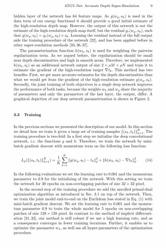
hidden layer of the network has 64 feature maps. As g(wg, sk) is used in thedata term of our energy functional it should provide a good initial estimate ofthe high-resolution depth map. However, the output of this network is not theestimate of the high-resolution depth map itself, but the residual gr(wg, sk), suchthat g(wg, sk) = gr(wg, sk) + sk. Learning the residual instead of the full outputaids the training procedure of the network [22], and has been applied before inother super-resolution methods [33, 36, 37].

The parameterization function h(wh, sk) is used for weighting the pairwiseregularization term. As we argued before, the regularization should be smallnear depth discontinuities and high in smooth areas. Therefore, we implementedh(wh, sk) as an additional network output of size 2 × ρM × ρN and train it toestimate the gradient of the high-resolution target ∇tk. This method has twobenefits: First, we get more accurate estimates for the depth discontinuities thanwhat we would get from the gradient of the high-resolution estimate g(wg, sk).Secondly, the joint training of both objectives in a single deep network improvesthe performance of both tasks, because the weights wh and wg share the majorityof parameters and only the parameters of the last layer, the output, differ. Agraphical depiction of our deep network parametrization is shown in Figure 2.

3.3 Training

In the previous sections we presented the description of our model. In this sectionwe detail how we train it given a large set of training samples {(sk, tk)}Kk=1. Thetraining procedure is two-fold: In a first step we initialize the deep convolutionalnetwork, i.e. the functions g and h. Therefore, we train the network by mini-batch gradient descent with momentum term on the following loss function:

Lp({(sk, tk)}Kk=1) =1

K

K∑k=1

‖g(wg, sk)− tk‖22 + ‖h(wh, sk)−∇tk‖22 . (14)

In the following evaluations we set the learning rate to 0.001 and the momentumparameter to 0.9 for the initializing of the network. With this setting we trainthe network for 30 epochs on non-overlapping patches of size 32× 32 pixel.

In the second step of the training procedure we add the unrolled primal-dualoptimization algorithm as introduced in Sec. 3.1 on top of the network. Then,we train the joint model end-to-end on the Euclidean loss stated in Eq. (1) withmini-batch gradient descent. We set the learning rate to 0.001 and the momen-tum parameter 0.9 to train the whole model for 5 epochs on non-overlappingpatches of size 128× 128 pixel. In contrast to the method of implicit differenti-ation [31, 32], our method is still robust if we use a high learning rate, and asa consequence converges in fewer training iterations. Further, it enables us tooptimize the parameter wλ, as well ass all hyper-parameters of the optimizationprocedure.


(a) rendered high-resolution ground-truth (b) corresponding mid-resolution input

Fig. 3. Examples of our generated depth maps. (a) visualizes the high-resolutionground-truth data. By resampling those depth maps with a scale factor ρ and addingdepth dependent noise we create the low-resolution input. (b) shows the mid-resolutioninput, which is the bilinear upsampled low-resolution data. Best viewed magnified inthe electronic version.

4 Evaluation

In this section we present an exhaustive experimental evaluation of the pro-posed ATGV-Net. First, we show how we generate a huge amount of trainingdata with accurate ground-truth needed to train the deep network. Then, wedemonstrate evaluation results on four standard benchmark datasets for depthmap super-resolution: Following [1, 13, 20], we evaluate our method on the noise-free Middlebury disparity maps Teddy, Cones, Tsukuba and Venus. Additionally,we show results for the Laserscan dataset as proposed in [1]. In a second evalu-ation we compare our results on the noisy Middlebury 2007 dataset as proposedin [29] and finally, we demonstrate the real-world applicability of our method onthe challenging ToFMark dataset [12].

We set the initial parameters of our model to α1 = 17, α0 = 1.2 for theregularization term, β = 9, γ = 0.85 for the anisotropic diffusion tensor, andwλ = 0.01 for all experiments. Further, we fix the number of iterations of theprimal-dual algorithm to 10.

4.1 Training Data

One challenge in training very deep networks is the need for a huge amountof training data. In [1, 13] the authors use a small set, i.e. 31 depth maps, ofsynthetic rendered images for training and in [32] the authors trained and testedtheir method on the synthetic New Tsukuba dataset [26]. Only very recentlylarger datasets with accurate depth maps have been released [17], or have beenadded to existing benchmarks [4]. In our method we also make use of syntheti-cally rendered data, but produce them in a much larger quantity.

For this purpose we implemented a ray-caster [2] that runs on the GPU andenables us to generate thousands of synthetic depth maps of high quality in afew minutes. For each image we randomly place between 24 and 42 rectangularcuboids and up to 3 spheres in a predefined volume. Further, we randomly scaleand rotate each solid to achieve an infinitely number of possible constellations.Then, we place a virtual camera at the origin of the coordinate system and cast


Table 1. Results on the noise-free Middlebury and Laserscan data. We report the erroras root mean squared error (RMSE) in pixel disparity for the Middlebury data and inmm for the Laserscan data, respectively. We highlight the best result in boldface andthe second best in italic.

×2 ×4 ×4

Cones Teddy Tsukuba Venus Cones Teddy Tsukuba Venus Scan21 Scan30 Scan42

NN 4.3772 3.2596 9.7968 2.1408 6.1236 4.5168 13.3248 2.9432 0.0177 0.0163 0.0396Bicubic 3.8392 2.7668 8.3648 1.8192 4.9544 3.5744 10.6960 2.3504 0.0132 0.0125 0.0326Diebel & Thrun [9] 2.9588 2.1060 6.4208 1.3624 4.5624 3.2040 8.7840 1.9408 − − −Ferstl et al. [12] 2.8240 2.1408 7.0592 1.2840 3.6372 2.5068 10.0128 1.4624 − − −Zeyde et al. [42] 2.7680 1.9616 6.1936 1.3200 3.8468 2.7812 8.7632 1.7592 0.0100 0.0093 0.0246Timofte et al. [36] 2.7872 1.9816 6.1280 1.3328 3.0256 3.0256 9.6304 1.9616 0.0106 0.0101 0.0264Aodha et al. [1] 4.5076 3.2988 9.6192 2.2088 6.0168 4.1036 13.3328 2.6920 0.0175 0.0170 0.0452Hornacek et al. [20] 3.9744 3.1640 9.2832 2.0592 5.5944 4.7828 11.6352 3.6008 0.0205 0.0179 0.0299Ferstl et al. [13] 2.4988 1.7588 5.6064 1.1464 3.7336 2.6680 7.8416 1.8096 0.0085 0.0083 0.0190

CNN only 1.0275 0.8201 2.3610 0.2266 3.0015 1.5330 6.4361 0.4219 0.0083 0.0082 0.0120CNN + ATGV-L2 1.0145 0.8374 2.3197 0.2720 2.9832 1.5175 6.4223 0.4124 0.0084 0.0083 0.0120ATGV-Net 1.0021 0.8155 2.3846 0.1991 2.9293 1.5029 6.6327 0.3764 0.0081 0.0081 0.0117

a ray for each pixel of the camera image. For each ray we compute the distancebetween the image plane and the closest surface it hits, or in the case it doesnot hit any surface, we return a maximum distance value for the background.In Figure 3 we illustrate two random examples of the more than 40, 000 depthmaps that we have generated with this method.

Given this generated depth maps as noise free ground-truth, we create the

low-resolution depth maps s(lr)k = ↓ρ tk for the network training by resampling

the generated ground-truth depth maps tk by the scale factor of ρ that is used inthe evaluation. Depending on the dataset, we additionally add depth-dependent

noise η(s(lr)k ) to the low-resolution depth map. Finally, we upsample this low-

resolution, probably noisy depth maps with bilinear interpolation to obtain our

mid-level representation sk = ↑ρ (s(lr)k + η(s

(lr)k )).

4.2 Clean Middlebury & Laserscan

In this first experiment we evaluate the performance of our proposed method onthe images Teddy, Cones, Tsukuba and Venus of the Middlebury dataset as in [1,13, 20]. The disparity is interpreted as depth and we test upsampling factors of×2 and ×4. Additionally, we evaluate on the Laserscan dataset images Scan21,Scan30 and Scan42 with an upsampling factor of ×4 as in [1, 13]. We compareour results to simple upsamling methods, such as nearest neighbor and bicubicupsampling, as well as to state-of-the-art depth upsampling methods that relyon an additional guidance image as input [9, 12]. Further, we show the results ofrecent sparse coding based approaches for single image super-resolution [42, 36],two approaches based on a Markov Random Field [1, 20] and a recent variationalapproach that uses sparse coding to estimate edge priors [13]. To demonstratethe effect of our variational model on top of the deep network, we show theresults of the high-resolution estimates of the network only (CNN only), theresults, where we add the variational model, but without joint training (CNN +ATGV-L2), and the results after end-to-end training (ATGV-Net).


(a) Input & GT (b) Timofte et al. [36] (c) Ferstl et al. [13] (d) CNN only (e) ATGV-Net

Fig. 4. Qualitative results for the noise-free Middlebury image Tsukuba, ρ = 4. (a)depicts the ground-truth and the input data. (b) and (c) show the results of state-of-the-art methods. (d) and (e) present the results of the deep network only and ourproposed model trained end-to-end. Best viewed magnified in the electronic version.

The results in terms of the root mean squared error (RMSE) are summa-rized in Table 1.1 We can clearly see that the deep network already achieves asignificant performance improvement compared to the other methods on bothdatasets and upsampling factors. Interestingly, we obtain even better results asthe methods [9, 12] that utilize an additional guidance image for the upsampling.This is especially pronounced in test samples with structures that are well simu-lated in the training data, such as Venus. Further, the variational model on topof the network slightly increases the performance and training the whole modelend-to-end gives the overall best results. One exception is the Tsukuba sample,where the results get slightly worse after end-to-end training. An explanationmight be that fine, elongated structures, e.g. near at the lamp of Tsukuba, arenot well represented in the training data. In the qualitative results, see Figure 4,we can further observe that the deep network with 10 layers achieves alreadyvery good results with sharper depth discontinuities compared to other methods.However, the improvement of the variational model on top of the deep networkis hardly visible. This becomes more apparent in the next experiment.

4.3 Noisy Middlebury

In this experiment we evaluate our method on the Middlebury disparity mapsArt, Books and Moebius with added depth dependent Gaussian noise to simulatethe acquisition process of a Time-of-Flight sensor, as proposed by Park et al. [29].

Therefore, we add to our low-resolution synthetic training data s(lr)k depth de-

pendent Gaussian noise of the form η(x) = N (0, σs(lr)k (x)−1), with σ = 651.

Exemplar training images are depicted in Figure 3. We report quantitative re-sults in Table 2 and visualize qualitative results in Figure 5.

We again compare our method to simple upsampling methods, such as nearestneighbor and bilinear interpolation. We compare our proposed method to otherapproaches that utilize an additional intensity image as guidance. Those methodsinclude the Markov Random Field based approach in [9], the bilateral filtering

1 Note that we present our results over the full disparity range [0, 255], as opposed toe.g. [13], where the disparities are scaled to a narrower range.


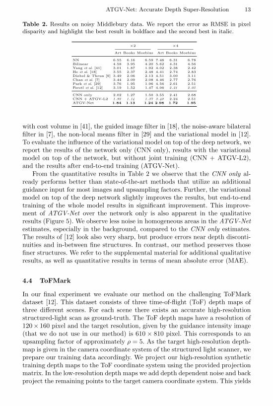
Table 2. Results on noisy Middlebury data. We report the error as RMSE in pixeldisparity and highlight the best result in boldface and the second best in italic.

×2 ×4

Art Books Moebius Art Books Moebius

NN 6.55 6.16 6.59 7.48 6.31 6.78Bilinear 4.58 3.95 4.20 5.62 4.31 4.56Yang et al. [41] 3.01 1.87 1.92 4.02 2.38 2.42He et al. [18] 3.55 2.37 2.48 4.41 2.74 2.83Diebel & Thrun [9] 3.49 2.06 2.13 4.51 3.00 3.11Chan et al. [7] 3.44 2.09 2.08 4.46 2.77 2.76Park et al. [29] 3.76 1.95 1.96 4.56 2.61 2.51Ferstl et al. [12] 3.19 1.52 1.47 4.06 2.21 2.03

CNN only 2.02 1.27 1.50 3.55 2.41 2.68CNN + ATGV-L2 1.93 1.14 1.37 3.40 2.24 2.51ATGV-Net 1.84 1.13 1.24 2.98 1.72 1.95

with cost volume in [41], the guided image filter in [18], the noise-aware bilateralfilter in [7], the non-local means filter in [29] and the variational model in [12].To evaluate the influence of the variational model on top of the deep network, wereport the results of the network only (CNN only), results with the variationalmodel on top of the network, but without joint training (CNN + ATGV-L2),and the results after end-to-end training (ATGV-Net).

From the quantitative results in Table 2 we observe that the CNN only al-ready performs better than state-of-the-art methods that utilize an additionalguidance input for most images and upsampling factors. Further, the variationalmodel on top of the deep network slightly improves the results, but end-to-endtraining of the whole model results in significant improvement. This improve-ment of ATGV-Net over the network only is also apparent in the qualitativeresults (Figure 5). We observe less noise in homogeneous areas in the ATGV-Netestimates, especially in the background, compared to the CNN only estimates.The results of [12] look also very sharp, but produce errors near depth disconti-nuities and in-between fine structures. In contrast, our method preserves thosefiner structures. We refer to the supplemental material for additional qualitativeresults, as well as quantitative results in terms of mean absolute error (MAE).

4.4 ToFMark

In our final experiment we evaluate our method on the challenging ToFMarkdataset [12]. This dataset consists of three time-of-flight (ToF) depth maps ofthree different scenes. For each scene there exists an accurate high-resolutionstructured-light scan as ground-truth. The ToF depth maps have a resolution of120× 160 pixel and the target resolution, given by the guidance intensity image(that we do not use in our method) is 610 × 810 pixel. This corresponds to anupsampling factor of approximately ρ = 5. As the target high-resolution depth-map is given in the camera coordinate system of the structured light scanner, weprepare our training data accordingly. We project our high-resolution synthetictraining depth maps to the ToF coordinate system using the provided projectionmatrix. In the low-resolution depth maps we add depth dependent noise and backproject the remaining points to the target camera coordinate system. This yields


(a) Input & GT (b) He et al. [18] (c) Ferstl et al. [12] (d) CNN only (e) ATGV-Net

Fig. 5. Qualitative results for the noisy Middlebury image Moebius, ρ = 4. (a) depictsthe ground-truth and the input data. (b) and (c) show the results of state-of-the-artmethods. (d) and (e) present the results of the deep network only and our proposedmodel trained end-to-end. Best viewed magnified in the electronic version.

Books Devil Shark

NN 30.46 27.53 38.21Bilinear 29.11 25.34 36.34Kopf et al. [23] 27.82 24.30 34.79He et al. [18] 27.11 23.45 33.26Ferstl et al. [12] 24.00 23.19 29.89

ATGV-Net 24.67 21.74 28.51

Table 3. Results on real Time-of-Flight data from theToFMark benchmark dataset. We report the error asRMSE in mm and highlight the best result in boldfaceand the second best in italic.

a very sparse depth map that we subsequently inpaint with bilinear interpolationto obtain our final mid-resolution training inputs.

We compare our results to simple nearest neighbour and bilinear interpola-tion, and three state-of-the-art depth map super-resolution methods that utilizean additional guidance image as input. The quantitative results are shown inTable 3 as RMSE in mm. Please see the supplemental material for qualitativeresults. Even on this difficult dataset we are at least on par with state-of-the-artmethods that utilize an additional intensity image as guidance input.

5 Conclusion

We presented a combination of a deep convolutional network with a variationalmodel for single depth map super-resolution. We designed the convolutional net-work to compute the high-resolution depth map, as well as the depth discontinu-ities. The network output was utilized in our variational model to further refinethe result. By unrolling the optimization procedure of the variational model, wewere able to optimize the joint model end-to-end, which lead to improved accu-racy. Further, we demonstrated the feasibility to train our method on a massiveamount of synthetic generated depth data and obtain state-of-the-art results onfour different benchmarks. Our model is especially useful if the low-resolutiondepth map contains noise, which is the case for most consumer depth sensors. Infuture work we plan to extend our model to depth data that contain larger areasof missing pixels, e.g. from structured light sensors. This is straight-forward bysetting wλ = 0 for areas where depth measurements are missing.

Acknowledgment: This work was supported by Infineon Technologies Austria

AG and the Austrian Research Promotion Agency under the FIT-IT Bridge program,

project #838513 (TOFUSION).


References

1. Aodha, O.M., Campbell, N.D., Nair, A., Brostow, G.J.: Patch Based Synthesisfor Single Depth Image Super-Resolution. In: European Conference on ComputerVision (ECCV) (2012)

2. Apple, A.: Some techniques for shading machine renderings of solids. In: Proceed-ings of the April 30–May 2, 1968, spring joint computer conference (1968)

3. Bredies, K., Kunisch, K., Pock, T.: Total Generalized Variation. SIAM Journal onImaging Sciences 3(3), 492–526 (2010)

4. Butler, D.J., Wulff, J., Stanley, G.B., Black, M.J.: A naturalistic open source moviefor optical flow evaluation. In: European Conference on Computer Vision (ECCV)(2012)

5. Chambolle, A., Pock, T.: A First-Order Primal-Dual Algorithm for Convex Prob-lems with Applications to Imaging. Journal of Mathematical Imaging and Vision40(1), 120–145 (2011)

6. Chambolle, A., Pock, T.: On the ergodic convergence rates of a first-order primal-dual algorithm. Mathematic Programming pp. 1–35 (2015)

7. Chan, D., Buisman, H., Theobalt, C., Thrun, S.: A Noise-aware Filter for Real-time Depth Upsampling. In: European Conference on Computer Vision Workshops(ECCVW) (2008)

8. Chen, L.C., Schwing, A.G., Yuille, A.L., Urtasun, R.: Learning Deep StructuredModels. In: Proceedings of the International Conference on Machine Learning(ICML) (2015)

9. Diebel, J., Thrun, S.: An Application of Markov Random Fields to Range Sensing.In: Proceedings of Conference on Neural Information Processing Systems (NIPS)(2005)

10. Domke, J.: Generic Methods for Optimization-Based Modeling. In: Proceedings ofthe International Conference on Artificial Intelligence and Statistics (AISTATS)(2012)

11. Dong, C., Loy, C.C., He, K., Tang, X.: Learning a Deep Convolutional Network forImage Super-Resolution. In: European Conference on Computer Vision (ECCV)(2014)

12. Ferstl, D., Reinbacher, C., Ranftl, R., Ruther, M., Bischof, H.: Image Guided DepthUpsampling using Anisotropic Total Generalized Variation. In: IEEE InternationalConference on Computer Vision (ICCV) (2013)

13. Ferstl, D., Ruther, M., Bischof, H.: Variational Depth Superresolution usingExample-Based Edge Representations. In: IEEE International Conference on Com-puter Vision (ICCV) (2015)

14. Girshick, R., Shotton, J., Kohli, P., Criminisi, A., Fitzgibbon, A.W.: Efficient Re-gression of General-Activity Human Poses from Depth Images. In: IEEE Interna-tional Conference on Computer Vision (ICCV) (2011)

15. Glasner, D., Bagon, S., Irani, M.: Super-Resolution from Single Image. In: IEEEInternational Conference on Computer Vision (ICCV) (2009)

16. Gupta, S., Girshick, R., Arbelaez, P., Malik, J.: Learning Rich Features from RGB-D Images for Object Detection and Segmentation. In: European Conference onComputer Vision (ECCV) (2014)

17. Handa, A., Patraucean, V., Badrinarayanan, V., Stent, S., Cipolla, R.: Under-standing Real World Indoor Scenes With Synthetic Data. In: IEEE Conference onComputer Vision and Pattern Recognition (CVPR) (2016)


18. He, K., Sun, J., Tang, X.: Guided Image Filtering. In: European Conference onComputer Vision (ECCV) (2010)

19. He, K., Zhang, X., Ren, S., Sun, J.: Deep Residual Learning for Image Recognition.In: IEEE Conference on Computer Vision and Pattern Recognition (CVPR) (2016)

20. Hornacek, M., Rhemann, C., Gelautz, M., Rother, C.: Depth Super Resolution byRigid Body Self-Similarity in 3D. In: IEEE Conference on Computer Vision andPattern Recognition (CVPR) (2013)

21. Izadi, S., Kim, D., Hilliges, O., Molyneaux, D., Newcombe, R., Kohli, P., Shotton,J., Hodges, S., Freeman, D., Davison, A., Fitzgibbon, A.: KinectFusion: Real-time3D Reconstruction and Interaction Using a Moving Depth Camera. In: ACM Sym-posium on User Interface Software and Technology (2011)

22. Kim, J., Lee, J.K., Lee, K.M.: Accurate Image Super-Resolution Using Very DeepConvolutional Networks. In: IEEE Conference on Computer Vision and PatternRecognition (CVPR) (2016)

23. Kopf, J., Cohen, M.F., Lischinski, D., Uyttendaele, M.: Joint Bilateral Upsampling.ACM Transactions on Graphics (TOG) 26(3), 96 (2007)

24. Krahenbuhl, P., Koltun, V.: Efficient Inference in Fully Connected CRFs withGaussian Edge Potentials. In: Proceedings of Conference on Neural InformationProcessing Systems (NIPS) (2012)

25. Kwon, H., Tai, Y.W., Lin, S.: Data-Driven Depth Map Refinement via Multi-scaleSpare Representations. In: IEEE Conference on Computer Vision and PatternRecognition (CVPR) (2015)

26. Martull, S., Peris, M., Fukui, K.: Realistic CG Stereo Image Dataset with GroundTruth Disparity Maps. In: International Conference on Pattern Recognition Work-shops (ICPRW) (2012)

27. Nagel, H.H., Enkelmann, W.: An Investigation of Smoothness Constraints for theEstimation of Displacement Vector Fields from Image Sequences. IEEE Transac-tions on Pattern Analysis and Machine Intelligence (TPAMI) 8(5), 565–593 (1986)

28. Ochs, P., Ranftl, R., Brox, T., Pock, T.: Bilievel Optimization with NonsmoothLower Level Problems. In: Scale Space and Variational Methods in Computer Vi-sion (SSVM) (2015)

29. Park, J., Kim, H., Tai, Y.W., Brown, M.S., Kweon, I.S.: High Quality Depth MapUpsampling for 3D-TOF Cameras. In: IEEE International Conference on Com-puter Vision (ICCV) (2011)

30. Ranftl, R., Gehrig, S., Pock, T., Bischof, H.: Pushing the Limits of Stereo UsingVariational Stereo Estimation. In: IEEE Intelligent Vehicles Symposium (2012)

31. Ranftl, R., Pock, T.: A Deep Variational Model for Image Segmentation. In: Ger-man Conference on Pattern Recognition (GCPR) (2014)

32. Riegler, G., Ranftl, R., Ruther, M., Bischof, H.: Joint Training of an ConvolutionalNeural Net and a Global Regression Model. In: Proceedings of the British MachineVision Conference (BMVC) (2015)

33. Schulter, S., Leistner, C., Bischof, H.: Fast and Accurate Image Upscaling withSuper-Resolution Forests. In: IEEE Conference on Computer Vision and PatternRecognition (CVPR) (2015)

34. Schwing, A.G., Urtasun, R.: Fully Connected Deep Structured Networks. In: arXivpreprint arXiv:1503.02351 (2015)

35. Shotton, J., Sharp, T., Kipman, A., Fitzgibbon, A., Finocchio, M., Blake, A.,Cook, M., Moore, R.: Real-time Human Pose Recognition in Parts from SingleDepth Images. In: IEEE Conference on Computer Vision and Pattern Recognition(CVPR) (2011)


36. Timofte, R., Smet, V.D., Gool, L.V.: Anchored Neighborhood Regression for FastExample-Based Super-Resolution. In: IEEE International Conference on ComputerVision (ICCV) (2013)

37. Timofte, R., Smet, V.D., Gool, L.V.: A+: Adjusted Anchored Neighborhood Re-gression for Fast Super-Resolution. In: Asian Conference on Computer Vision(ACCV) (2014)

38. Tompson, J., Jain, A., LeCun, Y., Bregler, C.: Joint Training of a ConvolutionalNetwork and a Graphical Model for Human Pose Estimation. In: Proceedings ofConference on Neural Information Processing Systems (NIPS) (2014)

39. Werlberger, M., Trobin, W., Pock, T., Wedel, A., Cremers, D., Bischof, H.:Anisotropic Huber-L1 Optical Flow. In: Proceedings of the British Machine Vi-sion Conference (BMVC) (2009)

40. Yang, J., Wright, J., Huang, T.S., Ma, Y.: Image Super-Resolution Via SparseRepresentation. IEEE Transactions on Image Processing 19(11), 2861–2873 (2010)

41. Yang, Q., Yang, R., Davis, J., Nister, D.: Spatial-Depth Super Resolution forRange Images. In: IEEE Conference on Computer Vision and Pattern Recogni-tion (CVPR) (2007)

42. Zeyde, R., Elad, M., Protter, M.: On Single Image Scale-Up Using Sparse-Representations. In: Curves and Surfaces (2010)

43. Zheng, S., Jayasumana, S., Romera-Paredes, B., Vineet, V., Su, Z., Du, D., Huang,C., Torr, P.: Conditional Random Fields as Recurrent Neural Networks. In: IEEEInternational Conference on Computer Vision (ICCV) (2015)

atgv-net: accurate depth super-resolution accurate depth super-resolution 3 only one low-resolution...

Documents