ATLAS & PS2

asteroid retrieval missiontarget detection capability study

prepared for NASA HEOMD

and the Jet Propulsion Laboratory

by

Robert Jedicke1 & Eva Schunova1

with

Peter Veres1, Larry Denneau1

2013 April 25

1Institute for Astronomy, University of Hawaii, 2680 Woodlawn Drive, Honolulu, HI,

96822, jedicke@ifa.hawaii.edu, 808.956.8080 (office), 808.988.3893 (fax)

– 2 –

1. Executive Summary

We have performed detailed good-fidelity simulations of the Asteroid Terrestrial-impact

Last Alert System (ATLAS, Tonry 2011) and the 2nd telescope of the Panoramic Survey

Telescope and Rapid Response System (PS2, e.g. Morgan et al. 2012) for detecting a set

of small asteroids that are accessible for robotic spacecraft retrieval. The small asteroids

(referred to as ‘pop1’ objects) have absolute magnitudes in the range 27 < H < 31

corresponding to diameters D ranging from 2 m< D < 30 m depending on their albedo.

They are on Earth-like heliocentric orbits with semi-major axis 0.7 AU< a < 1.45 AU,

eccentricity e < 0.2 and inclination i < 8◦. The combination of all the dynamical

requirements on the pop1 objects leaves a population with mean ∆v ∼ 4.2 km/s and

∆v . 6 km/s (Shoemaker and Helin 1978).

The ATLAS survey system is under construction and was proposed to include 2 sites

each with 1-4 telescopes. The system is expected to begin survey operations in a couple

years, i.e. early 2015, and is 100% funded by NASA’s NEOO program and 100% dedicated

to identifying NEOs. The nominal limiting magnitude is Vlim = 20.0 with the capability

of surveying 40,000 deg2/night — sufficient to image most of the night sky visible from

Hawaii 4× each night. Current designs for the ATLAS system may more than double that

capability with concomitant implications for the pop1 discovery rate. We modeled the

performance of a northern hemisphere version of ATLAS situated on Haleakala, Maui, HI,

and also a southern hemisphere realization situated on Cerro Tololo, Chile.

The PS2 survey system is the successor to the currently operational PS1 system (e.g.

Chambers 2007) on Haleakala, Maui, HI. PS2 may be operational in mid-2014 and its

survey operations are currently under negotiation. This study assumes that PS2 is a 100%

NEO-dedicated survey and actual performance should be scaled to the realized fraction of

the survey that will be suitable for identifying NEOs. PS2 will correct many of the issues

– 3 –

identified with PS1 and will benefit from a mature hardware and software system. It is

expected to have a limiting magnitude of Vlim = 22.0 and its 7 deg2 field-of-view and rapid

readout time will allow it to image about 3,600 deg2/night. While this is only about 1/11th

the coverage of the ATLAS system the 2 magnitudes greater depth allows the system to

detect the same objects ∼ 2.5× further away than ATLAS. The simulated survey images

the entire night sky visible from Hawaii twice per month.

For each of the simulated systems we studied the impact of both an increase and

decrease of 0.5 mag in the system limiting magnitudes. The decrease in the limiting

magnitude will occur if the systems fail to achieve their specified requirements. An increase

in the limiting magnitude might occur if the surveys were provided extra funding (this is

probably more applicable to ATLAS because it is still at an early enough stage that an extra

infusion of funds could modify the system design) or if they modified their survey strategy

(e.g. longer exposures concentrated near opposition). It must be noted that increasing the

exposure time will increase the limiting magnitude for the detection of stationary objects

but will have less impact on the limiting magnitude for the detection of moving pop1

objects.

Our results suggest that the ATLAS and PS2 surveys will be complementary in

the discovery of pop1 objects assuming that PS2 devotes 100% of its time to the NEO

search. ATLAS will be more effective at finding the pop1 objects but PS2 could improve

its capabilities if more aggressive software algorithms can be implemented to increase

the trail detection efficiency. The nominal pop1 discovery rate should be > 2/month for

ATLAS and about half that rate for the 100% NEO-dedicated PS2 system. Operating an

ATLAS-North and ATLAS-South system in parallel should increase the number of ATLAS

pop1 discoveries by ≥20%.

The pop1 objects are typically discovered in the direction towards opposition but there

– 4 –

is a broad distribution in the discovery location. This is mostly due to the phase angle effect

where objects are brightest towards opposition because they are nearly fully illuminated

(like the full moon). However, ATLAS’s synoptic nightly sky coverage allows it to discover

the pop1 objects at an average angular distance of about 40◦ from opposition while, perhaps

surprisingly, PS2 detects them at an average angular distance of ∼ 30◦ from opposition.

One serious problem was discovered while performing these simulations — the raw

predicted number of synthetic pop1 objects was far too low. The simulations suggest

that the existing PS1 survey should never have found any pop1 objects but it has already

identified several. We attribute the disparity to problems with the NEO orbit element and

size-frequency distribution in the size range of the pop1 objects. The NEO orbit element

model of Greenstreet and Gladman (2012) is strictly applicable only to kilometer-scale

NEOs and the Brown et al. (2002) size-frequency distribution could easily be uncertain by

a factor of a few to an order of magnitude. To reconcile the difference between the model

and the PS1 observations we simply normalized our simulations to the PS1 results. The

normalization factor of ∼ 8 is well within the expected systematic errors in our assumptions,

especially when considering that the PS1 pop1 detection efficiency is essentially unknown.

Most of the results presented herein are after accounting for this normalization factor.

Optical spectroscopic followup of the detected pop1 objects will be challenging. The

best opportunities for pop1 followup will be delivered by the ATLAS system. Only about

30% of the nominal ATLAS system pop1 detections are IRTF-recoverable and the fraction

for PS2 is only 10%. This is because the PS2 system’s deeper limiting magnitude allows

it to detect fainter objects when they are further away but these objects are less likely to

approach close to Earth and become bright enough for IRTF followup. This suggests that

PS2 may find 1-2 IRTF followup targets per year and ATLAS may find 5-10× that number.

The objects are typically available to IRTF for about 4 days during a week long period for

– 5 –

ATLAS and ∼ 12 days for the objects discovered by PS2.

The prospects for radar recovery of the pop1 objects is much better. Essentially all the

ATLAS-discovered pop1 objects are radar-detectable while slightly more than half of the

PS2-discovered objects are also radar-detectable. The objects are typically available for 2-3

weeks after discovery so that scheduling radar followup should not be onerous.

There is a strong bias towards discovering low-∆v objects with the current surveys and

this works to the advantage of the Asteroid Retrieval Mission.

– 6 –

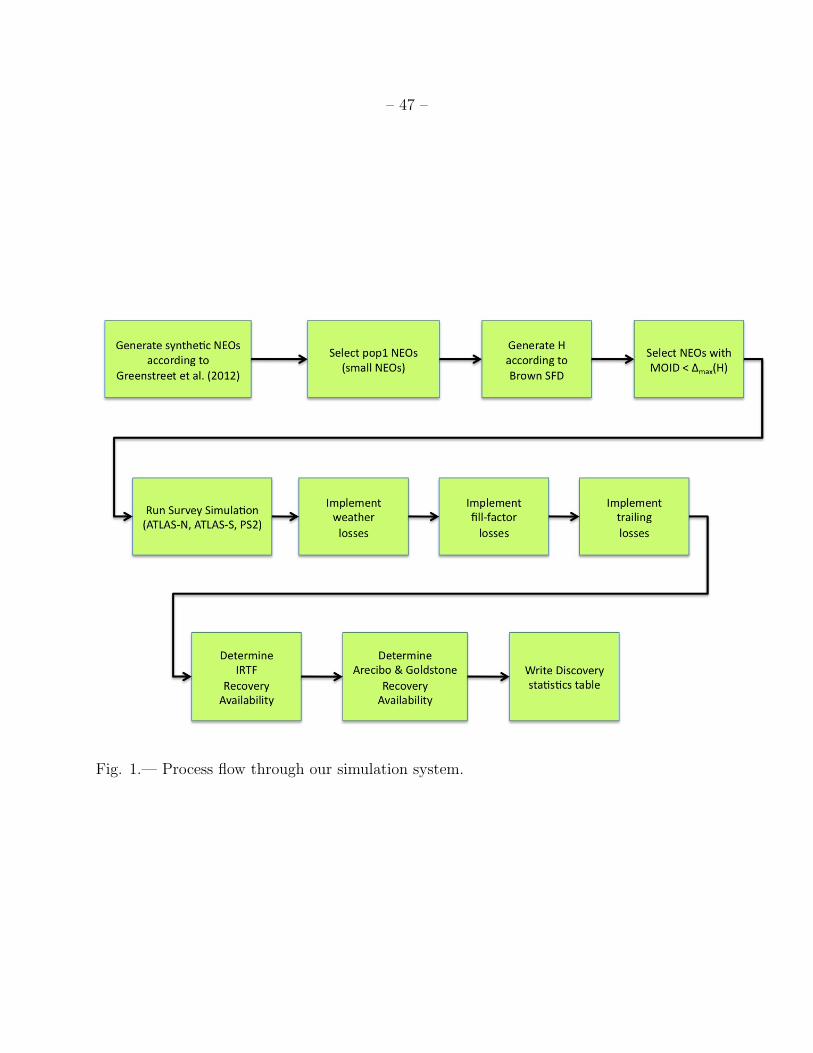
2. Processing pipeline

The high-level processing of the simulation is illustrated in fig. 1. Each of the steps is

described in detail below.

3. The NEO Model

We generated synthetic NEOs for this study according to the Greenstreet and Gladman

(2012) NEO orbit distribution that is currently the best orbit element model for the

NEOs. It corrects several deficiencies of the Bottke et al. (2002) NEO model including 1)

having higher resolution in semi-major axis (a), eccentricity (e), and inclination (i) and 2)

incorporating retrograde NEOs. The first point is particularly important to the detection

of NEOs accessible to human space missions because the Bottke et al. (2002) NEO model

includes relatively few bins covering the range of interesting NEOs.

The Greenstreet and Gladman (2012) NEO model uses the same weighting of the

different NEO sources as the Bottke et al. (2002) model but they used higher resolution,

higher statistics integrations. The differences between the orbit distributions in the models

are typically small as illustrated in fig. 2. The biggest difference is at small inclinations

(i < 10◦) where the Greenstreet and Gladman (2012) NEO model predicts fewer NEOs

than Bottke et al. (2002). This is in the opposite direction of the Mainzer et al. (2011) NEO

results that suggests that there are more NEOs at small inclination than predicted in the

Bottke et al. (2002) NEO model. So both the Bottke et al. (2002) and the Mainzer et al.

(2011) NEO models would yield more objects in the i < 10◦ bins of interest to this study.

– 7 –

3.1. Population 1 (pop1) - robotic retrieval mission targets

The synthetic NEOs were restricted to dynamically accessible mission targets (pop1)

based on 5 criteria provided by Chodas et al. (personal communication):

1. 0.7 AU < p < 1.05 AU

2. 0.95 AU < q < 1.45 AU

3. 2.99233 < TE < 3.01

4. e > −1.40591 aAU

+ 1.33562

5. e > +0.89132 aAU− 0.93588

where p = a(1 − e) and q = a(1 + e) are the object’s perihelion and aphelion distances

respectively, and TE is the object’s Tisserand parameter with respect to Earth given by

TE =AU

a+ 2 cos i

√a

AU(1− e2). (1)

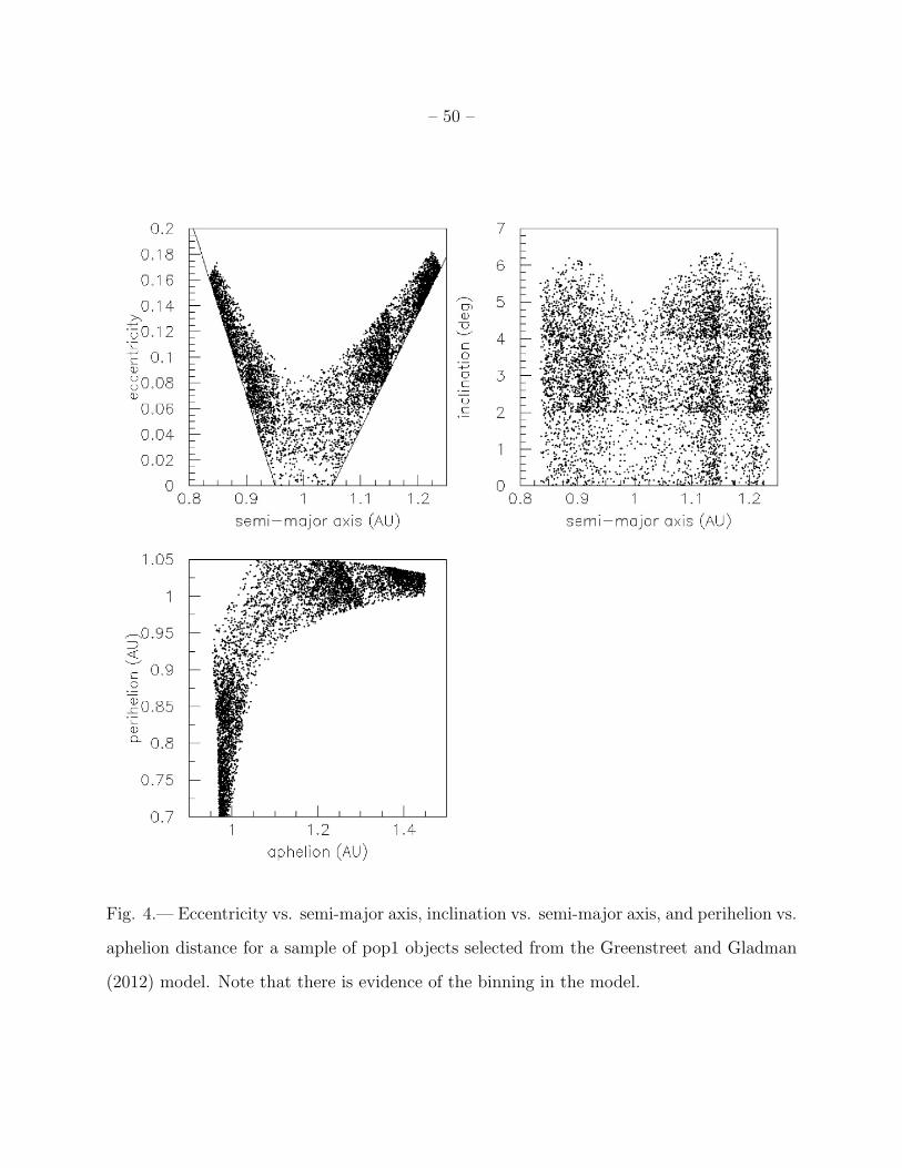
The dynamical cuts eliminate ∼99.9970% of NEOs in the model (fig. 3) and select

NEOs with semi-major axis close to Earth’s (a ∼ 1 AU), small eccentricity and low

inclination as illustrated in fig. 4. i.e. a fraction fpop1 = 0.000030 of NEOs pass the pop1

selection cuts. There is still evidence of the binning in the Greenstreet NEO model in the

latter figure.

3.2. smooth pop1

JPL was concerned about the residual binning evident in fig. 4 so we developed a

smoothed pop1 model that is used throughout the remainder of this report.

– 8 –

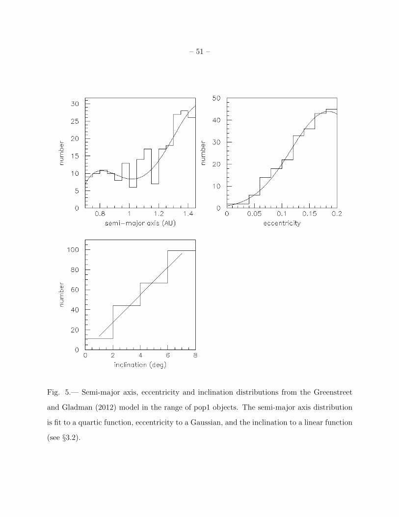
Figure 5 shows fits to the semi-major axis, eccentricity and inclination distributions

for the Greenstreet and Gladman (2012) NEO model in the range of pop1 objects. The

semi-major axis distribution was fit to a quartic function of the form

fa(a) = −893.337 + 3563.68 (a/AU)1 − 5141.61 (a/AU)2 + 3204.28 (a/AU)3 − 724.582 (a/AU)4,

(2)

the eccentricity to a gaussian of the form

fe(e) = 43.9115 exp−12( e−0.184212

0.067361)2

, (3)

and the inclination to a line forced to be zero at i = 0◦

fi(i) = 13.7509 (i/deg)1. (4)

Of course, the normalization of each of the functions is immaterial when generating random

a, e and i. We verified that the distributions in each parameter are roughly independent of

the others and then generated random sets of (a, e, i) and applied the pop1 dynamical cuts

to select NEOs in our smooth-pop1 sample. The distribution of the smooth-pop1 sample is

illustrated in fig. 6.

The purpose of the pop1 sample is to select NEOs with low ∆v as amply illustrated in

fig. 7. The pop1 NEOs are not representative of the orbit and ∆v distribution of the entire

NEO sample.

3.3. pop1 absolute magnitudes (H)

The absolute magnitudes of the pop1 NEOs is restricted to the range 27 ≤ H < 31

corresponding to diameters (D) in the range 2 m< D < 30 mdepending on their albedo. We

generated synthetic objects in each of eight 0.5 magnitude wide bins and assigned each an

absolute magnitude within the bin with a probability ∝ 100.54H appropriate for objects in

– 9 –

the size range as measured by Brown et al. (2002) (see fig. 9). The number of generated

pop1 NEOs (table C) was selected so that the survey simulation (see §4 below) would

detect about 100 objects per bin.

It is important to stress that the SFD of NEOs in the pop1 range is not well determined

with a factor of 10 uncertainty being entirely possible. While we were instructed to use

the Brown et al. (2002) NEO SFD there are other options as illustrated in fig. 8 (Stuart,

personal communication). The Mainzer 2011 distribution (Mainzer et al. 2011) was never

intended to be extrapolated down to the pop1 size range but is included to illustrate that

this type of extrapolation is typically unjustified. The Stuart 2001 distribution (Stuart

2001) is also an extrapolation to the pop1 size range from larger sizes but in this case could

be considered a lower bound to the number of objects in the pop1 range. The Brown 2002

distribution (Brown et al. 2002) is used in this work. We regard it is as best measurement

of the SFD in the pop1 range but would not be surprised to learn that the real distribution

is considerably different due to problems with debiasing the space sensor data or difficulties

in converting from the detected radiant energy to absolute magnitude. The Harris 2009

distribution is a fit to Alan Harris’ (unpublished but widely distributed) 2009 population

model using 3 straight lines. Finally, the Harris 2012 distribution is from Alan Harris’

(unpublished) 2012 population model.2 Finally, the JPL distribution corresponds to the

H = 24 distribution from fig. 20. It is included here because it i) appears to be a good

representation of the Harris 2012 distribution and ii) was the ‘original’ SFD used in the

preliminary powerpoint reports provided in this work effort.

2presented at the 2013 Planetary Defense Conference, Flagstaff, AZ

– 10 –

3.4. pop1 MOID selection

Most of the generated pop1 objects are impossible to detect with existing ground

based facilities because of their small sizes despite being selected for low ∆v. Thus, to

reduce the computation time for the survey simulations described in §4, we eliminated all

generated pop1 objects with Minimum Orbit Intersection Distance (MOID) greater than

the maximum distance at which an object with the generated absolute magnitude can be

detected. The maximum distance is (usually) determined by the object having its brightest

apparent magnitude (V ) when fully illuminated at opposition (i.e. zero phase angle (α),

Jedicke et al. 2003). Thus, we select objects from the pop1 sample that satisfy

V (H,∆ = MOID, α = 0) < Vlimit (5)

before running them through the survey simulation where Vlimit is the limiting magnitude

of the surveying system. This is equivalent to requiring that MOID < ∆(H) where ∆(H) is

the H-dependent maximum distance at which the object can be detected.

3.5. Population 2 (pop2) - Human Mission Targets

We were instructed by JPL to defer the pop2 study. They will not be mentioned again

in this report.

4. Survey Simulations

In this section we describe how we modeled the performance of the upcoming ATLAS

and PS2 surveys (see Tonry et al. (2012) and Morgan et al. (2012) respectively).

Each of the simulations is run in 3 different modes because neither of the surveys

is operational or fully constructed: a ‘nominal’ configuration at the expected limiting

– 11 –

magnitude, an ‘optimistic’ configuration with a limiting magnitude 0.5 mags higher than

expected, and a ‘pessimistic’ configuration with a limiting magnitude 0.5 mags lower than

expected. The ‘+0.5’ configuration might actually be achieved with system improvements

while the ‘-0.5’ configuration could reflect reality if there are problems with the system.

4.1. ATLAS

The Asteroid Terrestrial-impact Last Alert System (ATLAS, Tonry et al. 2012) has

the ambitious goal of surveying the entire night sky visible from its location 4×/night. The

design of the system is not yet finalized but it will use two sets of 1 to 4 small telescopes

with extremely wide fields-of-view (FOV). Each set may image 80 deg2 in each exposure

and reach Vlimit ∼ 20.0 (after stacking images from the telescopes within a set). Since the

system is not yet designed (let alone built) we have developed a survey simulation that

is relatively modest compared to what is expected. The baseline ATLAS system will cost

about $5M to design, build and operate over 5 years with all the funding provided by

NASA’s NEOO Program Office.

ATLAS is envisioned as an expandable system at a modest cost of roughly $1M/unit.

With more of these system distributed around the world in both longitude and latitude

it could achieve truly continuous coverage of the entire sky. With this in mind, we have

modeled both an ATLAS-North (ATLAS-N) and ATLAS-South (ATLAS-S) system as

described in the next subsection.

The key aspects of the nominal ATLAS-N survey simulation are

• situated on Halekala, Maui, at the location of PS1 (observatory code F51)

The actual location is still TBD but sites in Hawaii are most likely.

• 30 s exposures with 10 s readout time

– 12 –

• Vlimit = 20.0 (nominal)

we assume that the detection efficiency is constant for V < Vlimit and zero for

V ≥ Vlimit. The detection efficiency at bright magnitudes is determined by the fill

factor, image processing system and trailing losses described below.

• 40 deg2 FOV

This is the nominal design specification for the ATLAS system. They are currently

considering optical system designs that can deliver twice the FOV.

• 2 year simulation beginning 2015 January 1

• bore sites arranged so that FOVs cover the entire sky

• 10,000 deg2/night (i.e. imaged 4×)

Surveying most of the night sky every night.

• Transient Time Interval (TTI) ∼15 minutes The average time between

successive exposures at the same bore site.

• phase-dependent moon avoidance angle The minimum angular distance to the

moon increases with the moon’s phase.

• favor ecliptic fields

• no avoidance of galactic equator

• > 30◦ altitude

• nightly scheduling performed with Tools for Automated Observing (TAO3)

All the above are implemented in TAO so we have a nightly stream of bore site

3http://sites.mpc.com.br/holvorcem/tao/readme.html

– 13 –

locations and times specific to the night, moon, etc. Figure 10 shows the realized

survey pattern on four nights.

• Moving Object Processing System (MOPS, Denneau et al. (2013))

We used the PS1 MOPS to simulate the performance of the ATLAS survey. It takes

as input a list of boresites and times, FOV, the list of orbit elements and absolute

magnitudes for the objects, and determines which objects appear in which fields and

their apparent magnitudes and rates of motion. MOPS was designed to account for

many surveying factors like tracklet identification efficiency, fill-factor, weather, etc.,

but we accounted for these factors in post-MOPS processing as described in the next

three items.

• tracklet identification efficiency

Tracklets are sets of detections obtained in a short period of time (usually within 1-2

hours) associated with an individual object. They are the ‘units’ that are reported

to the MPC as candidate asteroid observations. Tracklet identification efficiency is a

combination of several factors including the camera’s fill factor, the stellar sky-plane

density, image processing detection efficiency, etc. ATLAS will use either a single

monolithic CCD or a small number of large CCDS so the fill factor, the fraction of

the focal plane instrumented with live pixels, will be close to unity. Most modern

asteroid surveys achieve very high detection efficiency for sources that are brighter

than the limiting magnitude when they appear on live pixels. Therefore, we assumed

95% detection efficiency for ATLAS brighter than the limiting magnitude — almost

certainly an underestimate.

• trailing losses

An object can move across the image so fast that it leaves a small ‘trail’ during even

short exposures. We refer to the reduction in tracklet identification efficiency due

– 14 –

only to its rate of motion as ‘trailing losses’. The effect is evident in real data as

illustrated for PS1 in fig. 12 — PS1 has never4 reported an NEO to the MPC that is

moving faster than 5◦/day. ATLAS will have ∼ 4′′ pixels and ∼ 3′′ PSF so trailing

losses begin when the source moves ∼ 2 pixels during the exposure. ATLAS will have

trail detection software so we expect that trailing losses will not be important for

objects moving at < 10◦/day. At faster rates of motion we assume a trailing loss as a

function of rate that is half that of the PS1 system as shown in fig. 11. We think this

is justified by the larger pixel scale and the anticipated use of trail-detection software.

• NEO identification

Contemporary asteroid surveys rely on the MPC NEO ‘digest’ score that is, essentially,

the probability that a real tracklet is a NEO if it can not be associated with a known

asteroid. The surveys typically submit and follow-up NEO candidates only when the

NEO digest score passes a threshold (like 50% or 90%). Thus, some NEOs ‘hide in

plain sight’ by virtue of being detected but having otherwise mundane locations and

rates of motion. This is not an issue for pop1 objects as shown in fig. 12 — virtually

all pop1 NEOs are moving so fast when they are detected that their digest score will

always be ∼ 100. We therefore do not need to ensure that the pop1 objects in our

simulations will be identified as NEOs.

• realistic weather & system downtime

4During the writing of this report, after more than two years of operations, the PS1 false

detection rate dropped low enough that the MOPS was able to relax an internal constraint

on a tracklet’s great circle residual (GCR). The relaxed threshold now allows faster moving

trails to be detected. Since the ATLAS & PS2 trailing losses are tied to the PS1 trailing

losses it will have little effect on the relative results reported here but will cause an (small)

increase in the overall discovery rate.

– 15 –

We use a realistic weather stream measured for Haleakala as shown in fig. 13. The

weather stream and observing metric are provided nearly continuously in 5 minute

time steps. We also know that over the course of roughly two years PS1 realized

a 53% observing efficiency i.e. 53% of the night time was used for observing after

accounting for all losses including weather and system downtime. We therefore utilize

the weather stream to select the 53% of half-night intervals that are ‘observable’ and

this simply requires that we require the observing metric to be > 0.07 as illustrated

in fig. 14. We note that it may not be fair to hobble ATLAS by forcing it to have the

same system downtime as PS1. ATLAS is a considerably simpler system that will be

designed from the outset for remote and robotic automated operations. We do not

anticipate that it will suffer from the same downtime as PS1

4.2. ATLAS-South

We have also implemented an ATLAS-South survey with exactly the same performance

characteristics as those described above except that the survey is located at Cerro Tololo

in Chile with observatory code 807. The survey pattern for a single full moon night is

illustrated in fig. 15 but we stress that this is not the pattern that would be used if there

really were multiple ATLAS sites in the two hemispheres. The current pattern has far too

much overlap with the ATLAS-North survey. A more rational coverage would require each

site to survey only north or south of the equator unless the other site is clouded out, in

which case the clear site should survey as much of the ecliptic as possible. Furthermore, the

entire sky will be easy to cover with ATLAS systems operating in both hemispheres and so

the entire sky could be imaged to a fainter limiting magnitude.

– 16 –

4.3. Caveats

Finally, we stress that we have purposefully under-estimated ATLAS tracklet detection

efficiency and the anticipated survey coverage, and over-estimated the system downtime so

as not to exaggerate the system’s simulated performance.

4.4. PS2 (Morgan et al. 2012)

PS2 is the successor to the currently operational Pan-STARRS prototype telescope

(PS1) on Haleakala, Hawaii (e.g. Chambers 2012). PS1 is widely believed to be an asteroid

survey but is actually a multi-purpose survey. The specifications of this study were that we

consider a NEO-dedicated PS2 system.

It is expected that PS2 will correct many of the issues discovered with the prototype

especially with regard to the CCD focal plane. Furthermore, it is expected that the image

processing pipeline will be improved and they should achieve a limiting magnitude of

V = 22.0 for their 1.8 m diameter primary.

The NEO-dedicated PS2 survey simulation was developed by PS2 personnel. The key

aspects of the nominal PS2 survey simulation are:

• situated on Halekala, Maui, at the location of PS1 (observatory code F51)

The real PS2 system will be located only a few tens of meters from the PS1 dome.

• 30 s exposures with 10 s readout time

• Vw,limit = 22.0 and Vz,limit = 21.0 (nominal)

PS2 will be outfitted with six filters but the survey simulation uses only two that

are optimized for NEO discovery under dark and moon-lit conditions — the wP1

and zP1 filters respectively. The wP1 filter is a very wide filter (= gP1 + rP1 + zP1)

– 17 –

optimized for asteroid detection while the zP1 filter is a near-IR filter suitable for high

sky-background conditions. We assume that the detection efficiency is constant for

V < Vlimit and zero for V ≥ Vlimit. The detection efficiency at bright magnitudes is

determined by the fill factor, image processing system and trailing losses described

below.

• 7 deg2 FOV

• 2 year simulation beginning 2015 January 1

• bore sites arranged so that FOVs cover the entire sky

The PS2 survey simulation includes special surveys of the ‘sweet spots’ for the

detection of Potentially Hazardous Objects (PHO). The sweet spots are two patches

of sky from 60◦ to 90◦ from the Sun and within 20◦ of the ecliptic.

• 900 deg2/night (i.e. imaged 4×/night)

The actual survey pattern and algorithm are complicated but the basic idea is that,

assuming perfect weather, the entire night sky is imaged on two nights in each

lunation. Visits to the same bore site within a lunation are separated by 3 nights.

• Transient Time Interval (TTI)

Typically ∼20 minutes except for images in the sweet spots with TTI∼8 min. The

TTI is also shortened slightly when surveying more than 90◦ from opposition and

more than 20◦ from the ecliptic.

• phase-dependent moon avoidance angle

At full moon wP1 survey fields are no closer than 120◦ to the moon while the zP1

survey fields are no closer than 60◦. The minimum angular separation of the field

from the moon decreases with the moon’s phase angle.

– 18 –

• no surveying within 10◦ of the galactic equator

The stellar sky-plane density is so high in the galactic plane at PS2’s limiting

magnitude that the asteroid detection efficiency drops dramatically.

• > 30◦ altitude

• nightly scheduling performed with Tools for Automated Observing (TAO5)

All the above are implemented in TAO so we have a nightly stream of bore site

locations and times specific to the night, moon, etc. Figure 16 shows the realized

survey pattern for a single night.

• Moving Object Processing System (MOPS, Denneau et al. 2013)

We used the PS1 MOPS to simulate the performance of the PS2 survey.

• tracklet identification efficiency

The realized PS1 tracklet efficiency at bright magnitudes is about 75% due mostly to

the fill factor — about 20% of the PS1 camera focal plane is occupied by gaps between

the CCDs, gaps on the CCDs themselves, and dead or inactive pixels. It is expected

that the PS2 camera will be cosmetically superior to the PS1 camera and we assumed

80% detection efficiency for PS2 detections brighter than the limiting magnitude.

• trailing losses

We assume that PS2 trailing losses will be similar to those measured for PS1 as shown

in fig. 11. Trailing losses begin at about 0.5◦/day due to the over-sampling of the PS2

PSF. (see footnote 4)

• NEO identification

PS2’s fainter limiting magnitude relative to ATLAS allows it to detect objects when

5http://sites.mpc.com.br/holvorcem/tao/readme.html

– 19 –

they are further away and therefore moving slower (in part alleviating trailing loss

affects described above) but they are still moving fast enough to be easily and mostly

unmistakably identified as NEOs. (See fig. 11.)

• realistic weather & system downtime

We use the same technique as described for ATLAS.

The PS2 survey simulation is in some respects of higher fidelity than the ATLAS

survey simulation. In particular it 1) uses separate filters and limiting magnitudes under

bright sky conditions when surveying close to the moon and 2) is based on the measured

pedigree of the operational PS1 system. We hope that PS2 will have a higher than 53%

overall operational efficiency but since this efficiency was applied to both the ATLAS and

PS2 simulations at least the relative performance of the two surveys in this study can be

easily compared.

5. Discussion

5.1. MOID selection effects

Only those pop1 objects that can possibly be detected by each of the systems described

above were pre-selected before running them through the survey’s MOPS simulation (based

on their MOID as described in §3.4). Figure 17 shows that roughly twice as many pop1

objects in each H bin are detectable by PS2 as compared to ATLAS by virtue of PS2’s

fainter limiting magnitude.

– 20 –

5.2. Detection efficiency & survey strategies

The pop1 objects are so small and pass by Earth so quickly that detecting them is very

difficult as illustrated in fig. 18 that shows the annual pop1 detection efficiency as a function

of H: εpop1(H). Our results suggest that only ∼0.1% of even the largest pop1 objects

are detected annually. We will show below that this results in very few pop1 discoveries

according to our simulations but there is an inconsistency between our model and the

current results from the PS1 system. There is good agreement between the calculated

efficiencies for ATLAS-North and South because the systems are essentially identical except

for their location and they survey mostly the same region of sky.

The ATLAS system has a higher overall pop1 detection efficiency than PS2 due to

being less sensitive to weather and trailing losses as illustrated in fig. 19. PS2 detects more

pop1 objects than ATLAS when we do not account for weather, system losses, tracklet

detection efficiency and trailing losses because it images the entire sky twice per month at

a greater depth than can be achieved by ATLAS each night. The problem is that PS2 will

not find the pop1 object if it is not in the field when the weather is good and the system is

operational or if it is moving too fast — and it only has a couple opportunities each month

to detect an object. While ATLAS does not image the sky as deeply, its nightly coverage of

the entire sky and large pixels yield an overall better efficiency than PS2.

There is nothing that can be done about the weather. Furthermore, as described above,

we expect both ATLAS and PS2 to have less system downtime than PS1 (that was used to

model the system behavior). But both effects will affect our ATLAS and PS2 simulations

identically and therefore not affect the relative performance comparison. Furthermore, in

our simulations there is only ∼ 15% difference in the tracklet detection efficiency (80% vs.

95%) and even if we invoke a claim that ATLAS will actually perform even better than the

nominal 95% it still makes only a small difference on the relative performance.

– 21 –

We think that PS2 has two opportunities for improving its overall efficiency: 1) modify

the survey strategy or 2) implement an aggressive trail identification algorithm. There are

numerous ways to modify the PS2 survey strategy to make it more effective for identifying

pop1 targets and the two most obvious are: A) eliminate field coverage far from opposition

and the ecliptic poles in order to provide 3× coverage of each field that remains and/or B)

decrease the exposure time to obtain more visits to each bore site during each lunation.

Option A should provide less susceptibility to weather and compensate for the tracklet

detection efficiency. Selecting optimal ranges in ecliptic longitude and latitude should be

relatively straightforward. Option B basically turns PS2 into ATLAS and is an ineffective

use of the system’s design characteristics.

There are also opportunities for improving ATLAS pop1 discovery performance. The

ATLAS survey specification in §4.1 reproduces the expectations at the time of the original

NASA NEOO proposal. Current ATLAS telescope and camera designs suggest that the

survey speed could be improved by a factor of ∼ 2. i.e. ATLAS could double the amount of

sky surveyed per night or increase the exposure time per field. Since the modeled ATLAS

survey already covers most of the sky of concern for pop1 objects it makes more sense to

devote the increased survey speed to increasing the system limiting magnitude. Similarly,

ATLAS could improve the survey limiting magnitude by foregoing surveying at high ecliptic

latitude or longitudes far from opposition. Furthermore, as mentioned in §4.2 there are

better ways to co-ordinate observations between an ATLAS-North and ATLAS-South

system that would certainly yield a higher pop1 detection efficiency.

5.3. Predicted annual discovery rates

The overall annual pop1 detection efficiency as a function of absolute magnitude with

respect to the entire NEO population is given by ε(H) = fpop1 εpop1(H). (fpop1 = 0.000030

– 22 –

was introduced in §3.1 and is the fraction of NEOs that pass the pop1 selection cuts.) The

annual number of detections in bins of width ∆H is simply

n(H) ∆H = ε(H) N(H) ∆H (6)

where n(H) and N(H) are the observed and actual number density of objects with respect

to H in the NEO population.

The debiased number of NEOs as a function of absolute magnitude has been measured

by various groups but the Statement of Work (see §A) requires that this study use the

distribution measured by Brown et al. (2002) for Earth-impacting asteroids. They calculate

that the cumulative number of impacting asteroids larger than diameter D (in meters) is

given by

logNimp(D) = c0 − d0 log(Dm

)(7)

with c0 = 1.57±0.03 and d0 = 2.70±0.08 valid for 22 < H < 30. We convert from diameter

to absolute magnitude (H) using

D

m=

106.1295

10H/5√p

(8)

where p is the geometric albedo. Our convention follows standard usage where an H = 17.75

object corresponds to an average diameter of 1 km which requires that p = 0.14421. We

then find that the cumulative number of objects with absolute magnitude < H impacting

Earth per year is given by

logNimp(H) = −16.117 + 0.54H. (9)

Brown et al. (2002) also claim that the annual impact frequency for NEOs is 2× 10−9/year

so that the total number of NEOs with absolute magnitude < H in the NEO population is

logNC(H) = −7.117 + 0.54H (10)

where NC represents the cumulative number as compared to the number density N(H)

from eq. 6. Clearly, N(H) ≡ dNC(H)/dH.

– 23 –

We consider the normalization factor (2×10−9/year) from the small impacting asteroids

to the entire NEO population to be a major source of systematic error in this analysis. The

normalization factor was calculated from ‘the average probability of impact for the 1,000

largest known near-Earth asteroids’ in 2002. Due to the different orbit distributions of the

small impacting asteroids compared to the large (and mostly non-impacting) 1,000 largest

known NEOs that certainly have a very different impact probability than the small NEOs

in this and the Brown et al. (2002) study.

Consider that the Bottke et al. (2002) NEO SFD for objects with H < 23 is ∝ 100.35

but the Brown et al. (2002) study states that the SFD is ∝ 100.54 for 22 < H < 30.

Furthermore, Mainzer et al. (2011) suggest that the SFD becomes shallower than the

Bottke et al. (2002) model for 100 m < D < 1,000 m. Thus, there must be a transition

from a shallow to steep slope somewhere in the range 22 < H < 27. Granvik et al. (2012)

reconciled the difference in slope between the Brown et al. (2002) and Bottke et al. (2002)

NEO distributions by assuming that the break in the SFD occurs at H = 24 as shown in

fig. 20. i.e. the SFD follows Bottke et al. (2002) to H = 24 and the Brown et al. (2002) SFD

for H ≥ 24. If the break and normalization were at smaller H than the predicted number

of objects at absolute magnitudes larger than the break would be higher (see fig. 20). If

the break occurs at H = 22 the predicted number of NEOs increases by a factor of ∼ 2.5

compared to the number with a break at H = 24. There is about a factor of 6 difference

between the nominal Brown et al. (2002) SFD and the model with the break at H = 24.

Despite our concerns about the NEO model normalization our model from the

Statement of Work is the nominal Brown et al. (2002) SFD. Using that distribution, our

calculated annual detected number of pop1 objects as a function of absolute magnitude

(n(H), see fig. 21) peaks near H = 28.25 for ATLAS and near H = 27.25 for PS2 and shows

that ATLAS detects more pop1 objects than PS2 in every bin. The peak exists because

– 24 –

the detection efficiency decreases faster with H than the size of the population increases

and the location of the peak is determined by each system’s efficiency (see fig. 18). The

total annual number of discovered pop1 objects is predicted to be about 4 for the ATLAS

systems and ∼ 2 for PS2 as shown in fig. 22.

5.4. Comparison with PS1 observations

‘The PS1 system limiting magnitude’ is difficult to quote because the survey uses

multiple filters under widely varying observing conditions but the limiting magnitude in

the wP1 filter, used to make the vast majority of asteroid discoveries, is . 21.5 in V . It can

therefore be loosely compared with the results of the PS2-0.5 survey simulation described

herein. PS1 has actually discovered 3 NEOs that meet the pop1 criteria even but our

PS2-0.5 simulation predicts that it should discover ∼ 0.7/year. At first glance the values are

not necessarily inconsistent but we will show that they reveal a discrepancy in the fidelity

of our simulation.

First, PS1 is not a dedicated NEO survey. While the non-NEO survey component of

the PS1 survey can be used to identify NEOs it is much less efficient at doing so and the

fraction of time devoted to the solar system survey has changed with time. We estimate

that the effective fraction of PS1 solar system survey time is about 25% i.e. the system

could discover about 4× more NEOs if it was dedicated to the NEO program. Furthermore,

it is difficult to quantify the effective duration of the survey because the system has ramped

up its capabilities over time. We estimate that the effective survey duration is about 2 years

for comparison with this work. Thus, a NEO-dedicated PS1 telescope might have detected

6 pop1 objects per year (= 3 pop1 object in 2 years of surveying at 25% efficiency6). Note

6Our estimates for the effective surveying time and NEO survey fraction are simply

– 25 –

that this is ∼ 8× our predicted value!7

We regard the factor of 8 discrepancy between our PS2-0.5 simulation and the actual

PS1 performance as explicable by factors already described above:

1. a factor of ∼ 4 due to the differences between the Greenstreet and Gladman (2012),

Bottke et al. (2002) and Mainzer et al. (2011) orbit distribution models (particularly

at low inclination),

2. the adoption of the Bottke et al. (2002) orbit distribution model suitable for large

NEOs for the small pop1 objects,

3. our estimate of the ‘effective’ PS1 NEO survey efficiency and comparison to the

PS2-0.5 survey simulation.

5.5. Normalized annual discovery rates

We have implemented a normalization to our predicted annual discovery rates to

account for the discrepancy between our simulation and the PS1 pop1 discoveries such

that the PS2-0.5 simulation discovers 6 pop1 objects annually as shown in fig. 23. With

educated guesses. Both may be in error by up to about 50%.

7Careful readers will note that the preliminary reports had much larger disparities. There

are 2 reasons for the drop from the previously reported value of ∼ 100 to ∼ 8: 1) we identified

a bug in the MOPS software that caused a failure to load all the zP1 survey fields (a factor

of 2) and 2) we adopted the Brown et al. (2002) NEO SFD rather than the Granvik et al.

(2012) implementation of the Brown et al. (2002) NEO SFD (another factor of 6 as described

in §5.3).

– 26 –

this normalization factor the nominal PS2 system identifies more than one pop1 object per

month while ATLAS identifies about half a dozen per month.

We note that if ATLAS can achieve an increase in limiting magnitude by 0.5 mags that

it will double its discovery rate to about a dozen pop1 targets per month. A similar 0.5 mag

increase in the PS2 limiting magnitude will more than double its pop1 discovery rate but

even so it will find only about as many pop1 objects as the nominal ATLAS system.

The normalized annual discovery rate as a function of absolute magnitude is shown in

fig. 23.

5.6. ATLAS-North + ATLAS-South

Figures 21-24 show that our simulated crude version of a dual-hemisphere ATLAS

system would detect 10-20% more pop1 objects than either single-hemisphere system. We

stress that our estimate is clearly a lower limit to the benefits of dual-hemispheric coverage

as our ATLAS-North and ATLAS-South survey strategies do not take advantage of the

other as described in §4.2. The impact of our inefficient survey strategy is two-fold: 1)

when one site is weathered out the other site can survey the most important region of the

sky near opposition ensuring ‘continuous’ surveying and 2) when both sites are operational

they can avoid each other’s survey region to maximize the total sky coverage or increase

the survey depth to identify pop1 objects at larger distances.

5.7. Survey overlap

ATLAS has been promoted as being complementary to the Pan-STARRS NEO effort

and this claim is supported by our analysis of the overlap in detected objects between the

– 27 –

ATLAS-North, ATLAS-South and PS2 systems in each of the nominal and nominal±0.5

configurations as illustrated in fig. 25. In this analysis we assume that all 3 systems are

surveying at the same time in the same configuration with respect to their nominal limiting

magnitudes.

The ATLAS-North and ATLAS-South systems each uniquely identify about 10% of all

the detected pop1 objects regardless of the limiting magnitude configuration. Furthermore,

about 11% of all the discovered pop1 objects are detected by all 3 systems, again without

regard to configuration. The biggest effect is that as the systems’ limiting magnitudes

are increased in tandem from -0.5 mag, to 0 mag, to +0.5 mag the fraction of uniquely

discovered objects by PS2 increases from 19%, to 22%, and 28% respectively.

5.8. ∆v selection effects within pop1

Figure 26 shows that there is a strong selection effect for the simulated systems to

discover lower ∆v objects within pop1. This is presumably because the lower ∆v objects

are moving slower when near the Earth and spending more time in the surveys’ search

volumes.

However, fig. 27 shows that the mean ∆v of synthetic discovered objects with the

ATLAS-S+0.5 system is close to the pop1 average and there is not a strong trend with

absolute magnitude. We note that the faintest/smallest two H bins have the smallest

RMS and the mean in those bins is many σ from the pop1 mean but it is not clear that

the standard error on the mean should be considered as a definitive test given that that

distribution is strongly non-guassian.

In other words, the systems identify objects with lower ∆v but the ∆v distribution is

only weakly dependent on the absolute magnitude.

– 28 –

5.9. IRTF spectroscopic follow up

Once a pop1 object is identified it will be important to obtain follow up spectroscopic

observations. We were instructed to examine the follow up windows with the IRTF after

discovery. We used an IRTF spectroscopic follow up limiting magnitude of V = 18.5 (Bin

Yang, personal communication).

Figure 28 shows several observable properties for a particular pop1 object after

discovery with the nominal ATLAS-North system. The general behavior is common to

many objects discovered by the system that subsequently become observable with IRTF.

The discovered object typically (but not always) becomes brighter — it usually must do so

in order to be brighter than the IRTF limiting magnitude unless the object happens to be

discovered near peak brightness. Furthermore, because the objects are so small, they are

typically discovered near opposition at small phase angles and large solar elongation.

We were initially surprised that the fraction of targets discovered by each system that

are accessible for followup by IRTF decreases as the system’s limiting magnitude increases

(see fig. 29). We attribute this effect to the fact that a deeper limiting magnitude allows

detection of the small objects at larger distances but this does not mean that they will

necessarily enter into the followup volume accessible to IRTF. Indeed, the objects discovered

with the more capable systems are less likely to be recovered by IRTF.

The effect is particularly important for the followup of objects discovered by PS2. It’s

2 magnitude fainter limit allows it to detect small objects when they are much further

away but this means that a larger fraction of the discovered objects are too faint for IRTF

followup.

The total number of followup targets increases with the system limiting magnitude

despite the reduction in the fraction of recoverable objects as illustrated in fig. 29. The

– 29 –

simulations suggest that the ATLAS systems might detect about one pop1 object per month

that can be characterized with IRTF but the PS2 system might detect only a few per year.

Once an object is available for IRTF followup it is desirable that it remain available for

as long as possible. We find that the average window ‘width’ for IRTF followup is about

4 to 5 days independent of the survey system and the survey system limiting magnitude.

There is a small but statistically significant decrease in the average window length as the

survey system’s limiting magnitude improves (goes to larger values). We again attribute

this to the fact that the improved systems detect the objects when they are further away

and less likely to spend time in the volume accessible to IRTF.

The ATLAS-South performance is typically slightly less than the ATLAS-North

performance because some of the pop1 objects detected in the southern hemisphere simply

never appear in the northern hemisphere’s sky or have dropped in brightness before they

do.

Finally, the length of time during which IRTF followup is possible is different than

the time between discovery and the closing of the followup window (window ‘duration’) as

illustrated in fig. 30. The duration is significantly longer for the PS2 survey because when

PS2 discovers a pop1 object that will become observable with IRTF, it does so when the

objects are further away and the window opens up a few days after discovery. This could

provide an advantage over ATLAS in that it allows more time to react to the discovery to

schedule the followup.

The relative fraction of discovered pop1 objects discovered by the ATLAS and PS2

systems as shown in fig. 25 would change dramatically in favor of the ATLAS system if

IRTF followup was required.

– 30 –

5.10. Arecibo & Goldstone radar follow up

Paul Chodas provided us some pseudo-code to calculate radar signal-to-

noise ratio (SNR) for both the Arecibo and Goldstone facilities but we never

succeeded in converting it to operational code. Instead, we resorted to a sim-

ple fit to the Arecibo SNR from a figure available online from Lance Benner

(http://echo.jpl.nasa.gov/ lance/snr/far asnr18.gif) reproduced in fig. 31.

We found that we can reproduce the H = 26 curve (most appropriate to the lowest range

of the pop1 objects) using an S-class albedo of p = 0.155 and

SNRArecibo =1

2.5

(Dkm

)2(AU∆

)4

(11)

where D is the object’s diameter and ∆ is its geocentric distance. Substituting for D we

find

SNRArecibo =1

2.5

( 1347

10H/5√p

)2(AU∆

)4

(12)

In our simulations we use p = 0.14421 as in §5.3. Since the area of the Goldstone

facility is about 1/20th the area of the Arecibo facility we assume that

SNRGoldstone =SNRArecibo√

20(13)

since we are assuming a minimum SNR=10. We understand that the actual usable area of

the Arecibo facility is dependent on the target object’s altitude, and we understand that

there are many other factors that affect a small asteroid’s SNR at both facilities, but we

think that the formulae above provide enough fidelity for this study.

A large fraction of the discovered pop1 objects will be recoverable with the radar

facilities as illustrated in fig. 34, unlike optical spectroscopic followup with IRTF. Indeed,

70-80% of all ATLAS-discovered pop1 objects will be recoverable with Arecibo and

essentially 100% of them will be recoverable from Goldstone. The fraction of PS2

– 31 –

discoveries that are radar-recoverable is not as good but is still in the 50-60% range.

The high-fraction translates into a large annual number of recoverable objects with

perhaps 2-3 ATLAS-discovered objects recoverable per month and about 1 PS2-discovered

object/month.

Mirroring the optical followup, those objects that are detected by PS2 tend to be

visible in longer windows and for longer durations than those detected by ATLAS. However,

the difference is not large and in each case there are about 3 weeks of time after discovery

by either system to schedule radar followup.

It appears that radar recovery and physical characterization of the pop1 objects should

be straightforward.

6. Conclusions

We think that the major utility of this study is the relative performance of the different

surveys because it is clear that there are issues with both the NEO orbit and size-frequency

distribution in the pop1 size range. We needed to employ a large and ad-hoc normalization

to our survey simulations to match the observed PS1 discovery rate that is probably

due to both the inadequate orbit distribution of the small objects and their SFD. The

normalization factor was ∼ 8 but even this value could be an underestimate because of all

the incorporated uncertainties. We would not be surprised if the actual correction factor is

an order of magnitude larger.

The ATLAS system(s) will make a significant contribution to the pop1 discovery effort.

Their all-sky every-night coverage combined with their large pixel scale is well-suited to the

detection of the fast moving pop1 objects. The systems’ modest limiting magnitude (at

least in comparison to the PS2 survey) turns out to be an extra benefit when restricting

– 32 –

the desirable pop1 objects to those that are accessible for spectroscopic followup by IRTF.

Since ATLAS has Vlim = 20.0 any discovered object must be brighter than this limit and

is all the more likely to become brighter than the IRTF’s limiting magnitude during its

apparition.

The PS2 system will also contribute to the pop1 discovery effort and contribute a

sub-set of objects that it can uniquely identify by virtue of its deeper limiting magnitude

if a significant fraction of its time can be devoted to the effort (this study assumed that

it would be a 100% NEO survey). On the other hand, its Vlim = 22.0 allows it to detect

the small pop1 objects when they are far from Earth and on trajectories that make them

less likely to reach an apparent magnitude accessible for IRTF followup. The PS2 camera

has a relatively small pixel scale of ∼ 0.25′′ so the PSF is over-sampled and this makes

trailing losses particularly acute. An aggressive and CPU-intensive software algorithm

could be deployed to identify trails corresponding to pop1 objects to compensate for the

trailing losses. Furthermore, it is likely that PS2 would be more efficient at detecting pop1

objects if it was dedicated specifically to identifying them rather than all NEOs. e.g. the

survey pattern could be targeted towards opposition with more repeat visits to the same

location and/or longer exposure times (though the latter would exacerbate the trailing loss

problem).

Detecting the small and fast moving pop1 objects is a challenging endeavor and

obtaining spectroscopic followup makes the problem all the more difficult. While 20-50% of

the ATLAS-detected pop1 objects come within range of the IRTF facility only 5-20% of the

PS2-detected objects achieve the same (depending on the limiting magnitude configuration

of the survey simulation).

Finally, we would like to take the opportunity of directing the reader’s attention to

the work of Granvik et al. (2012) who claim that there exists a population of asteroids in

– 33 –

temporary geocentric orbits. These objects have very low ∆v and they predict that there

one or two 1 to 2 meter diameter objects in orbit around Earth at any time. Like the

heliocentric pop1 objects, the geocentric ‘minimoons’ would make excellent targets for an

asteroid retrieval mission. The problem with the minimoons is detecting them. But we

believe that dedicated, targeted surveys could be developed to identify the most interesting

largest objects in orbit.

– 34 –

A. Appendix: Comparison to original SOW

This section compares the delivered products to the last statement of work on 2013

Jan 10 titled Jedicke work statement 01102013.

Population 1 The set of NEOs to be output should have absolute magnitudes

in the range 31 <= H <= 27, and orbits with v∞ < 2.6 km/s with respect to

Earth. A simple estimate of the v∞ could be computed from the objects

Tisserand parameter TE with respect to the Earth. In (a, e, i) orbital

element phase space, these objects would likely be bounded by the limits

0.8 < a < 1.3 AU, e < 0.3 and i < 5◦.

COMPLETE The pop1 specification was substantially modified during a series of

emails and telecons with Chodas, Chesley and others. The final pop1 specification

described in §3.1 was delivered on 2013 March 1.

Population 2 The set of NEOs to be output should have absolute magnitudes

in the range 19.5 <= H <= 25, and orbits that allow missions with a total

∆v < 5 km/s. The cutoff limits in (a, e, i) orbital phase space should be

enlarged to 0.6 <= a <= 2 AU, e <= 0.7, i <= 20◦, which are the limits used

by Zimmer & Messerschmid (2011)8.

N/A We were instructed to ignore pop2 as described in §3.5.

0 The main output of the simulations will be a realistic estimate of the expected

discovery rates of these target bodies as a function of size bins.

8We were unable to locate this reference.

– 35 –

COMPLETE The discovery rates for all systems are discussed in §5.3 and §5.5.

A The NEOSSat-1.0 NEO population model (Greenstreet and Gladman 2012)

should be used, since it has finer resolution in (a, e, i) Population space

than the old Bottke et al. (2002) model.

COMPLETE We have used the Greenstreet and Gladman (2012) as described

in §3 but implemented an improvement to remove residual binning as described in §3.2.

B The discovery simulations should be run for an all-sky ATLAS survey and a

deeper NEO-dedicated Pan-STARRS-2 ecliptic survey.

COMPLETE We have implemented both as described in §4.

C The statistics of the length of time between discovery and the closing of the

radar, photometry and spectrophotometry windows should be examined.

COMPLETE We provide an analysis of the IRTF and radar followup windows in

§5.9 and §5.10 respectively.

D The ATLAS and Pan-STARRS limiting magnitude assumptions should be

varied to surround the expected limiting magnitude. For example, the

ATLAS limiting magnitudes should include values of 19.5, 20.0, and 20.5.

COMPLETE We have implemented nominal and nominal±0.5 mag limiting magni-

tudes for each of the ATLAS-North, ATLAS-South and PS2 systems as described in §4.

– 36 –

E The benefit of a second ATLAS system — possibly in southern hemisphere

— should be examined.

COMPLETE We have performed all our simulations for a southern hemisphere

ATLAS system as described in §4.2.

F The simulation should be for at least one month for both surveys (the same

month) but it is desirable to simulate at least one year and preferably two

years of operations.

COMPLETE We have performed all our simulations for two years for all three

surveys as described in §4.

G The simulation should make the best effort at incorporating the effects of

weather on the survey strategy.

COMPLETE We have incorporated a full weather stream into our models that also

incorporates system downtime as described in §4

H The final report should provide synthetic results for the observability of at

least 1,000 NEOs in the desired range of absolute magnitudes.

COMPLETE The nominal+0.5 simulations provide results for 1,225 pop1 objects.

The nominal simulations yielded 625 pop1 objects. The nominal-0.5 simulations

yielded 279 objects.

I The discovery rate should be estimated separately in bins 0.5 absolute

magnitudes width.

– 37 –

COMPLETE The discovery rate was measured separately in bins 0.5 absolute

magnitudes width as described in §5.3 and §5.5.

J Discovery rate statistics should be plotted against v∞ bins in order to assess

whether the lower v∞ objects are more likely to be discovered than the

higher v∞ objects.

COMPLETE Discussions with the JPL NEO office after the creation of the State-

ment of Work (SoW) suggested that v∞ was not a useful measure for this study. The

SoW was not re-written so we have interpreted this requirement in terms of ∆v which

we believe to be a more useful independent parameter. The analysis is described in §5.8.

K The output of each simulation should be a file of data for each simulated

object that gets discovered. The file should include orbital elements,

discovery circumstances and observability circumstances for the relevant

discovery follow-up.

COMPLETE The tabular results are available at

http://www.ifa.hawaii.edu/users/jedicke/data/ARM analysis results.zip.

The delivered package is described in §C.

B. Delivery Schedule

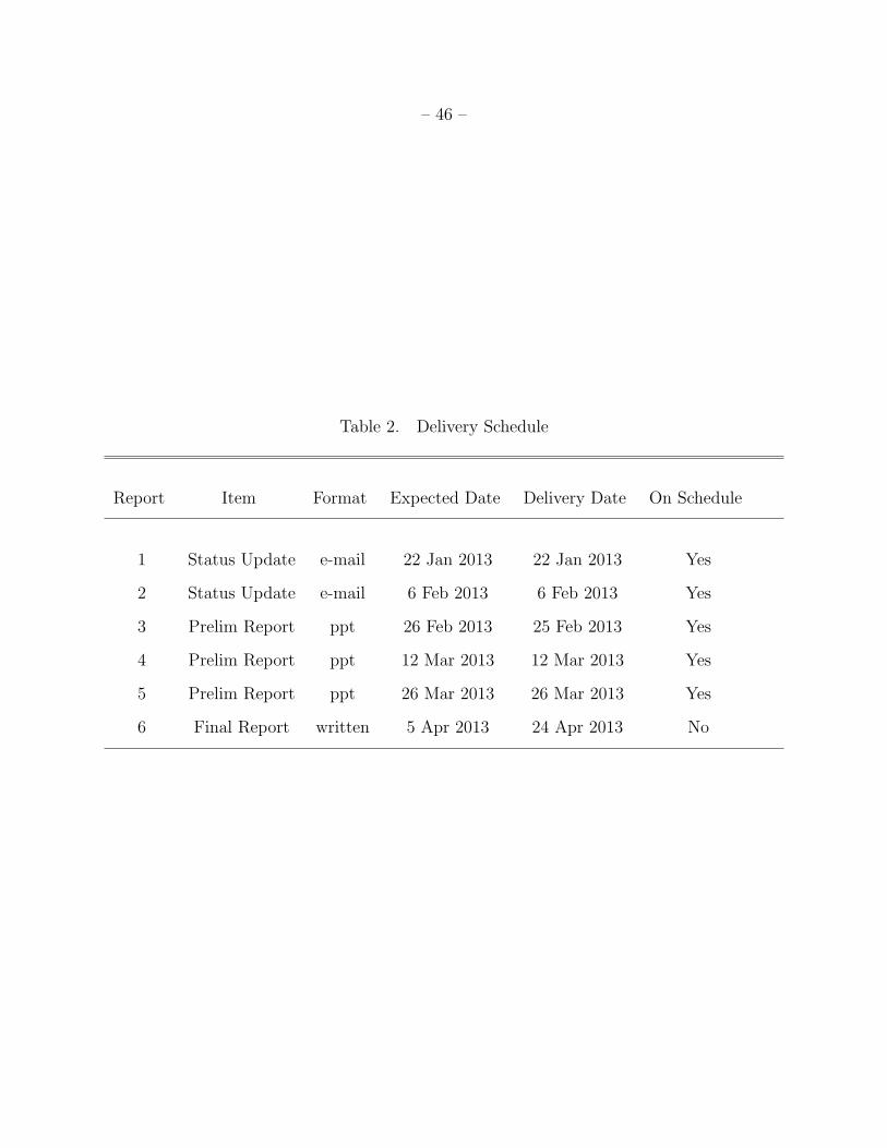
The agreed delivery schedule and actual delivery date are provided in table 2. The

only report that was delivered late is this final report. We were told that delivery by the

morning of 2013 April 24 would be acceptable. A trivial update of the final report was

– 38 –

provided the next day — 2013 April 25.

C. Delivered Package

All the results of this study are available at

http://www.ifa.hawaii.edu/users/jedicke/data/ARM analysis results.zip.

The zip file contains the following directories:

OUTPUT-TABLES

Figures-Atlas-North-V19.5

Figures-Atlas-North-V20.0

Figures-Atlas-North-V20.5

Figures-Atlas-South-V19.5

Figures-Atlas-South-V20.0

Figures-Atlas-South-V20.5

Figures-PS2-21.5

Figures-PS2-V22.0

Figures-PS2-V22.5

Jedicke-Schunova-ATLAS-PS2-ARM-study-2013-04-25.pdf

Jedicke-Schunova-ATLAS-PS2-ARM-study-2013-04-24.xlsx

generate-greenstreet-neos-v2.1.py

The top level directory contains this report, an excel spreadsheet

(Jedicke-Schunova-ATLAS-PS2-ARM-study-2013-04-25.xlsx)

containing most of the data and many of the figures in this report, and the python code

(generate-greenstreet-neos-v2.1.py) required to generate the smoothed pop1 NEOs

from the Greenstreet and Gladman (2012) NEO model. The python code usage can be

found by executing the command python generate-greenstreet-neos-v2.1.py -h.

– 39 –

The Figures* directories include figures showing the observability circumstances for

all the synthetic pop1 objects discovered with each survey simulation from the perspective

of followup with IRTF, Arecibo and Goldstone. We think the nomenclature for the 9 survey

simulation sub-directories is self-explanatory.

The OUTPUT-TABLES directory contains the following survey-simulation sub-directories:

ATLAS N 19.5 SMOOTH POP1/

ATLAS N 20.0 SMOOTH POP1/

ATLAS N 20.5 SMOOTH POP1/

ATLAS N+S/

ATLAS S 19.5 SMOOTH POP1/

ATLAS S 20.0 SMOOTH POP1/

ATLAS S 20.5 SMOOTH POP1/

PS2 21.5 SMOOTH POP1/

PS2 22.0 SMOOTH POP1/

PS2 22.5 SMOOTH POP1/

Each survey simulation directory contains 3 files. For instance, the

ATLAS N 19.5 SMOOTH POP1 directory contains:

POP1.ATLAS.195 complete table.dat

README.txt

pop1.atlas.195 complete table.dat.paw

The *.dat file is the output table for objects discovered in the simulation corresponding

to the current directory. The *.paw can be ignored. It is essentially the *.dat file with

all non-numeric characters removed. It could be useful for software that is not capable of

handling non-numeric values.

– 40 –

The README.txt file provides a short description of the current simulation and the

meaning of the 22 columns in the *.dat file. The columns are:

1. Name of object

2. Discovery date [MJD]

3. V at discovery [mag]

4. Topocentric Opposition-centered longitude at discovery [deg]

5. Topocentric Opposition-centered lattitude at discovery[deg]

6. Orbit epoch [MJD]

7. Semi-major axis [AU]

8. Eccentricity

9. Inclination [deg]

10. Argument of perihelion [deg]

11. Longitude of Ascending node [deg]

12. Main anomaly [deg]

13. Absolute magnitude [mag]

14. IRTF window - Beginning [MJD]

15. IRTF window - End [MJD]

16. IRTF window - Length [days]

17. Arecibo window - Beginning [MJD]

18. Arecibo window - End [MJD]

19. Arecibo window - Length [days]

20. Goldstone window - Beginning [MJD]

21. Goldstone window - End [MJD]

22. Goldstone window - Length [days]

– 41 –

Acknowledgments

We thank Richard Wainscoat, co-lead on the PS1 Inner Solar System Key Project, and

John Tonry, the ATLAS PI, both from the University of Hawaii’s Institute for Astronomy,

for their insights into operations envisioned for PS2 and ATLAS respectively. We thank

Scott Stuart, MIT Lincoln Laboratory, for helpful discussions on the pop1 size-frequency

distribution.

– 42 –

REFERENCES

Bottke, W. F., A. Morbidelli, R. Jedicke, J.-M. Petit, H. F. Levison, P. Michel, and

T. S. Metcalfe 2002. Debiased Orbital and Absolute Magnitude Distribution of the

Near-Earth Objects. Icarus 156, 399–433.

Bottke, W. F., Jr., A. Cellino, P. Paolicchi, and R. P. Binzel 2002. Asteroids III. Asteroids

III .

Brown, P., R. E. Spalding, D. O. ReVelle, E. Tagliaferri, and S. P. Worden 2002. The flux

of small near-Earth objects colliding with the Earth. Nature 420, 294–296.

Chambers, K. C. 2007. The PS1 System and Science Mission. In American Astronomical

Society Meeting Abstracts, Volume 39 of Bulletin of the American Astronomical

Society, pp. #142.06.

Chambers, K. C. 2012. Pan-STARRS1 Science Mission, Status and Results. In American

Astronomical Society Meeting Abstracts #220, Volume 220 of American Astronomical

Society Meeting Abstracts, pp. #107.04.

Denneau, L., R. Jedicke, T. Grav, M. Granvik, J. Kubica, A. Milani, P. Veres, R. Wainscoat,

D. Chang, F. Pierfederici, N. Kaiser, K. C. Chambers, J. N. Heasley, E. A. Magnier,

P. A. Price, J. Myers, J. Kleyna, H. Hsieh, D. Farnocchia, C. Waters, W. H.

Sweeney, D. Green, B. Bolin, W. S. Burgett, J. S. Morgan, J. L. Tonry, K. W.

Hodapp, S. Chastel, S. Chesley, A. Fitzsimmons, M. Holman, T. Spahr, D. Tholen,

G. V. Williams, S. Abe, J. D. Armstrong, T. H. Bressi, R. Holmes, T. Lister,

R. S. McMillan, M. Micheli, E. V. Ryan, W. H. Ryan, and J. V. Scotti 2013. The

Pan-STARRS Moving Object Processing System. ArXiv e-prints .

Granvik, M., J. Vaubaillon, and R. Jedicke 2012. The population of natural Earth satellites.

Icarus 218, 262–277.

– 43 –

Greenstreet, S., and B. Gladman 2012. High-inclination Atens ARE Rare. In AAS/Division

for Planetary Sciences Meeting Abstracts, Volume 44 of AAS/Division for Planetary

Sciences Meeting Abstracts, pp. 305.05.

Jedicke, R., A. Morbidelli, T. Spahr, J. M. Petit, and W. F. Bottke 2003. Earth and

space-based NEO survey simulations: prospects for achieving the spaceguard goal.

Icarus 161, 17–33.

Mainzer, A., T. Grav, J. Bauer, J. Masiero, R. S. McMillan, R. M. Cutri, R. Walker,

E. Wright, P. Eisenhardt, D. J. Tholen, T. Spahr, R. Jedicke, L. Denneau,

E. DeBaun, D. Elsbury, T. Gautier, S. Gomillion, E. Hand, W. Mo, J. Watkins,

A. Wilkins, G. L. Bryngelson, A. Del Pino Molina, S. Desai, M. Gomez Camus, S. L.

Hidalgo, I. Konstantopoulos, J. A. Larsen, C. Maleszewski, M. A. Malkan, J.-C.

Mauduit, B. L. Mullan, E. W. Olszewski, J. Pforr, A. Saro, J. V. Scotti, and L. H.

Wasserman 2011. NEOWISE Observations of Near-Earth Objects: Preliminary

Results. ApJ 743, 156.

Morgan, J. S., N. Kaiser, V. Moreau, D. Anderson, and W. Burgett 2012. Design differences

between the Pan-STARRS PS1 and PS2 telescopes. In Society of Photo-Optical

Instrumentation Engineers (SPIE) Conference Series, Volume 8444 of Society of

Photo-Optical Instrumentation Engineers (SPIE) Conference Series.

Shoemaker, E. M., and E. F. Helin 1978. Earth-approaching asteroids as targets for

exploration. In D. Morrison and W. C. Wells (Eds.), NASA Conference Publication,

Volume 2053 of NASA Conference Publication, pp. 245–256.

Stuart, J. S. 2001. A Near-Earth Asteroid Population Estimate from the LINEAR Survey.

Science 294, 1691–1693.

Tonry, J. L. 2011. An Early Warning System for Asteroid Impact. PASP 123, 58–73.

– 44 –

Tonry, J. L., C. W. Stubbs, K. R. Lykke, P. Doherty, I. S. Shivvers, W. S. Burgett, K. C.

Chambers, K. W. Hodapp, N. Kaiser, R.-P. Kudritzki, E. A. Magnier, J. S. Morgan,

P. A. Price, and R. J. Wainscoat 2012. The Pan-STARRS1 Photometric System.

ApJ 750, 99.

This manuscript was prepared with the AAS LATEX macros v5.2.

– 45 –

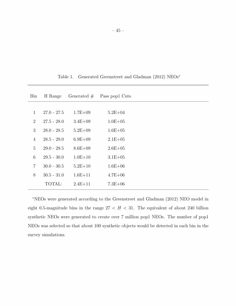
Table 1. Generated Greenstreet and Gladman (2012) NEOs∗

Bin H Range Generated # Pass pop1 Cuts

1 27.0 - 27.5 1.7E+09 5.2E+04

2 27.5 - 28.0 3.4E+09 1.0E+05

3 28.0 - 28.5 5.2E+09 1.6E+05

4 28.5 - 29.0 6.9E+09 2.1E+05

5 29.0 - 29.5 8.6E+09 2.6E+05

6 29.5 - 30.0 1.0E+10 3.1E+05

7 30.0 - 30.5 5.2E+10 1.6E+06

8 30.5 - 31.0 1.6E+11 4.7E+06

TOTAL: 2.4E+11 7.3E+06

∗NEOs were generated according to the Greenstreet and Gladman (2012) NEO model in

eight 0.5-magnitude bins in the range 27 < H < 31. The equivalent of about 240 billion

synthetic NEOs were generated to create over 7 million pop1 NEOs. The number of pop1

NEOs was selected so that about 100 synthetic objects would be detected in each bin in the

survey simulations.

– 46 –

Table 2. Delivery Schedule

Report Item Format Expected Date Delivery Date On Schedule

1 Status Update e-mail 22 Jan 2013 22 Jan 2013 Yes

2 Status Update e-mail 6 Feb 2013 6 Feb 2013 Yes

3 Prelim Report ppt 26 Feb 2013 25 Feb 2013 Yes

4 Prelim Report ppt 12 Mar 2013 12 Mar 2013 Yes

5 Prelim Report ppt 26 Mar 2013 26 Mar 2013 Yes

6 Final Report written 5 Apr 2013 24 Apr 2013 No

– 47 –

Fig. 1.— Process flow through our simulation system.

– 48 –

Fig. 2.— Semi-major axis, eccentricity and inclination distributions from the Greenstreet

and Gladman (2012) and Bottke et al. (2002) NEO models.

– 49 –

Fig. 3.— Eccentricity vs. semi-major axis distribution for 190, 499 NEOs generated from

the Greenstreet and Gladman (2012) model. The binning in the model is evident along the

right edge of the distribution where p = a(1 − e) = 1.3 AU. The five red dots are the only

mission accessible targets according to the 5 criteria provided in §3.

– 50 –

Fig. 4.— Eccentricity vs. semi-major axis, inclination vs. semi-major axis, and perihelion vs.

aphelion distance for a sample of pop1 objects selected from the Greenstreet and Gladman

(2012) model. Note that there is evidence of the binning in the model.

– 51 –

Fig. 5.— Semi-major axis, eccentricity and inclination distributions from the Greenstreet

and Gladman (2012) model in the range of pop1 objects. The semi-major axis distribution

is fit to a quartic function, eccentricity to a Gaussian, and the inclination to a linear function

(see §3.2).

– 52 –

Fig. 6.— Semi-major axis, eccentricity and inclination distributions from the smooth-pop1

sample for comparison with fig. 4. Note that there are no bin edge effects within the sample.

– 53 –

Fig. 7.— Fractional distribution of ∆v for the pop1-smooth sample (left) and NEOs from

the entire Greenstreet and Gladman (2012) model. ∆v was calculated using the algorithm

of Shoemaker and Helin (1978).

– 54 –

Fig. 8.— (courtesy of Scott Stuart, MIT Lincoln Laboratory) Cumulative absolute magni-

tude distribution according to several NEO models. See §3.3 for a detailed discussion.

– 55 –

Fig. 9.— Normalized fraction of objects in each H bin in the pop1 NEO sample showing

that within each H bin the objects are distributed according to the Brown et al. (2002) NEO

size-frequency distribution (∝ 100.54(H−24)) appropriate for objects with H > 18. i.e. within

a bin the ratio of the number of objects on the right and left sides of the 0.5 mag wide bin is

1.86 ∼ 100.54×0.5 and the total number of objects increases dramatically as H increases from

left to right.

– 56 –

Fig. 10.— ATLAS-North survey pattern on 4 nights. Each red square represents a single

boresite that is imaged 4 times with roughly a TTI between each image. The squares each

represent the central portion of the 40 deg2 image so that the sky between each red square is

fully imaged. The red line represents the ecliptic while the blue line represents the galactic

equator. The positions of the Sun, Moon and planets are represented by little images of

each near the ecliptic. The top 2 images are for the winter nights of 22 and 6 January 2015

respectively. The bottom 2 images are for the summer nights of 19 and 3 June respectively.

The left images are at new moon and the images on the right are at full moon. Note that

long winter nights allow the opportunity to cover most of the sky but on shorter summer

nights the survey coverage does not go as far north with the more southerly ecliptic.

– 57 –

Fig. 11.— (top left) Apparent V magnitude vs. rate of motion (ω) for asteroids detected with

the PS1 telescope. i.e. real asteroids detected by the actual PS1 system. Main belt asteroids

dominate the number statistics for ω . 0.5◦/day. The red line represents the empirical

trailing loss limit above which asteroids are too faint to be reliably detected. Trailing losses

begin at about 0.5◦/day. ALL THE REMAINING FIGURES CORRESPOND TO THE

SIMULATED NOMINAL+0.5 LIMITING MAGNITUDE SYSTEMS (top right). Apparent

V magnitude vs. rate of motion for synthetic pop1 NEOs detected by PS2 in this study.

(bottom left) Apparent V magnitude vs. rate of motion for synthetic pop1 NEOs detected

by ATLAS-North in this study. (bottom right) Apparent V magnitude vs. rate of motion

for synthetic pop1 NEOs detected by ATLAS-South in this study.

– 58 –

Fig. 12.— (top left) Rates of motion for asteroids detected with the actual PS1 telescope.

Note the logarithmic number scale. The spike at small rates is due to main belt asteroids

that dominate the number statistics. The NEOs extend to the highest rates of motion

though PS1 has not yet reported a NEO with a rate > 5◦/day (see footnote 4). ALL

THE REMAINING FIGURES CORRESPOND TO THE SIMULATED NOMINAL+0.5

LIMITING MAGNITUDE SYSTEMS INCLUDING THE EFFECTS OF WEATHER, FILL

FACTOR, AND TRAILING. (top right) Rates of motion for synthetic pop1 NEOs detected

by PS2 in this study. (bottom left) Rates of motion for synthetic pop1 NEOs detected

by ATLAS-North in this study. (bottom right) Rates of motion for synthetic pop1 NEOs

detected by ATLAS-South in this study. The distribution for ATLAS-South is essentially

identical to that for ATLAS-North as expected.

– 59 –

Fig. 13.— PS1 observing metric as a function of time (top) and a histogram of the average

observing metric in half-night intervals (bottom). The metric can be roughly interpreted as:

1.0 — photometric, 0.5 — acceptable, 0.0 — no observing.

– 60 –

Fig. 14.— Cumulative fractional observing metric in half-night intervals. More than 53% of

half-nights have an average observing metric of ≥ 0.07.

– 61 –

Fig. 15.— Survey pattern for the full moon night of 2015 Jan 6 for the ATLAS-South

survey. The figure is identical to the upper right panel in fig. 10 except for the survey being

performed from Cerro Tololo in Chile (observatory code 807). The southerly location of the

ATLAS-S site means that the Moon, located well above the equator, is not such a problem

for the ATLAS-South site on this night. More of the fields are close to the equator and the

survey is truncated close to the south celestial pole.

– 62 –

Fig. 16.— (top) PS2 survey pattern for an entire lunation. PS2 will image each boresite

4×/night and 2×/lunation. The entire visible night sky is imaged in the absence of losses

due to weather. (bottom) PS2 survey pattern for the full moon night of 6 January 2015 —

the same night as the upper right panel in fig. 10. The blue fields are imaged in the zP1

band due to their proximity to the moon while the white fields are imaged in wP1. The

‘patchiness’ compared to fig. 10 is due to PS2’s smaller FOV and the attempt to image the

entire sky each lunation.

– 63 –

Fig. 17.— The fraction of pop1 objects that become bright enough to be detectable by

ATLAS and PS2 based only on the objects’ MOID and absolute magnitude. i.e. about 40%

of pop1 objects with H ∼ 30.25 are detectable by the PS2+0.5 system.

– 64 –

Fig. 18.— Annual pop1 detection efficiency as a function of absolute magnitude for the

nominal (top) and nominal∓0.5 mag ATLAS-North, ATLAS-South and PS2 survey systems.

– 65 –

Fig. 19.— Raw number of synthetic pop1 discoveries in a 2 year simulation for the nomi-

nal+0.5 versions of the ATLAS-North, ATLAS-South and PS2 survey systems. Each column

represents the number of discoveries at the specified step in the pipeline. ‘Detected’ refers to

raw detections from the simulation — the object appeared in a field of view and was brighter

than the limiting magnitude. ‘w/ weather & system’ is the number of discoveries after ac-

counting for weather and system downtime. ‘w/ tracklet efficiency’ accounts for losses due

to tracklet detection efficiency. ‘w/trailing loss’ accounts for trailing losses due to the motion

of the object during an exposure.

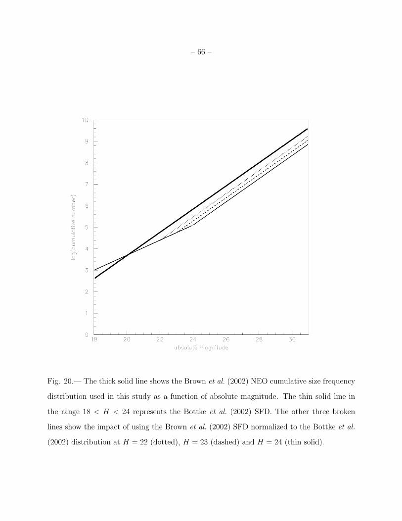
– 66 –

Fig. 20.— The thick solid line shows the Brown et al. (2002) NEO cumulative size frequency

distribution used in this study as a function of absolute magnitude. The thin solid line in

the range 18 < H < 24 represents the Bottke et al. (2002) SFD. The other three broken

lines show the impact of using the Brown et al. (2002) SFD normalized to the Bottke et al.

(2002) distribution at H = 22 (dotted), H = 23 (dashed) and H = 24 (thin solid).

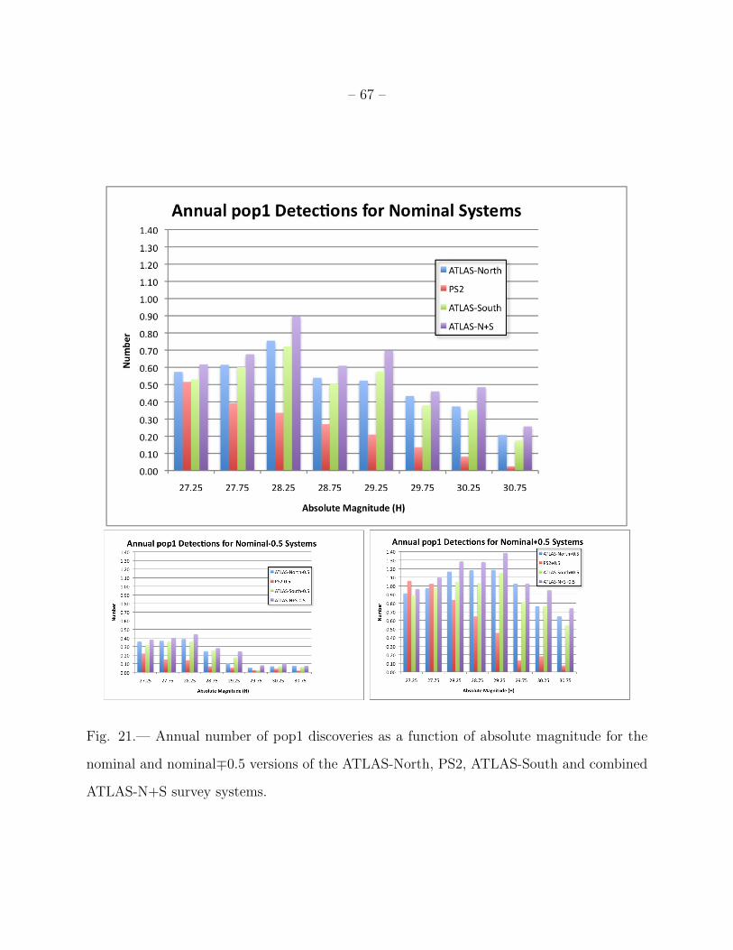
– 67 –

Fig. 21.— Annual number of pop1 discoveries as a function of absolute magnitude for the

nominal and nominal∓0.5 versions of the ATLAS-North, PS2, ATLAS-South and combined

ATLAS-N+S survey systems.

– 68 –

Fig. 22.— Annual number of pop1 discoveries for the nominal and nominal±0.5 versions of

the ATLAS-North, PS2, ATLAS-South and combined ATLAS-N+S survey systems

– 69 –

Fig. 23.— Normalized annual number of pop1 discoveries for the nominal and nominal±0.5

versions of the ATLAS-North, PS2, ATLAS-South and combined ATLAS-N+S survey sys-

tems. The PS2-0.5 system now discovers 6 objects to be consistent with the estimated

annualized 6 pop1 objects discovered by the PS1 system. NOTE: the scale on this figure is

4× the scale on fig. 22.

– 70 –

Fig. 24.— Normalized annual number of pop1 discoveries as a function of absolute magnitude

for the nominal and nominal±0.5 versions of the ATLAS-North, PS2, ATLAS-South and

combined ATLAS-N+S survey systems.

– 71 –

Fig. 25.— All these figures illustrate the fraction of detected pop1 objects that are unique

to a particular survey or identified by 2 of the surveys assuming that all the surveys were

operating at the same time. i.e. the top (nominal) pie chart assumes that the nominal

ATLAS-North, ATLAS-South and PS2 systems are all operational at the same time and in

this circumstance about 22% of all detected objects are uniquely detected by PS2. The 3

different pie charts represent the results for the nominal and nominal∓0.5 configurations.

About 11% of all objects are detected by all 3 surveys regardless of the configuration with

respect to nominal.

– 72 –

Fig. 26.— Normalized relative efficiency for detecting pop1 objects with the PS2+0.5 system

as a function of ∆v (Shoemaker and Helin 1978). i.e. this is not the absolute efficiency relative

to the pop1 objects.

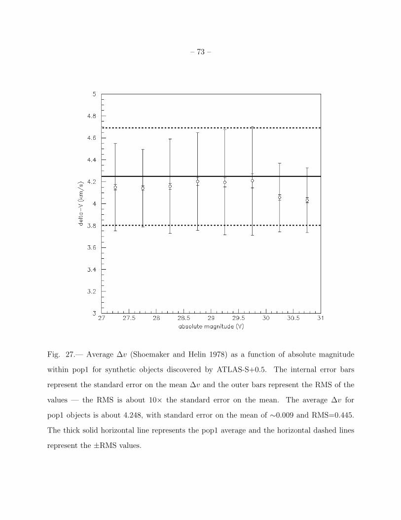
– 73 –

Fig. 27.— Average ∆v (Shoemaker and Helin 1978) as a function of absolute magnitude

within pop1 for synthetic objects discovered by ATLAS-S+0.5. The internal error bars

represent the standard error on the mean ∆v and the outer bars represent the RMS of the

values — the RMS is about 10× the standard error on the mean. The average ∆v for

pop1 objects is about 4.248, with standard error on the mean of ∼0.009 and RMS=0.445.

The thick solid horizontal line represents the pop1 average and the horizontal dashed lines

represent the ±RMS values.

– 74 –

Fig. 28.— The black dots (some times dense enough that they appear to be a line) in

each panel represent the properties of an individual NEO for 100 days after discovery by

the nominal ATLAS-North system. The red lines represent the detection threshold for that

property with the IRTF for spectroscopic followup and the gray regions represent when an

object is unobservable with IRTF. This object is observable with the IRTF for only 3 days

beginning a few days after discovery by the nominal ATLAS system. The red star and

triangles in the Dec. vs. R.A. and topocentric ecliptic latitude vs. topocentric ecliptic

longitude figures represent the location of the object on the day of discovery and on the

100th day after discovery respectively.

– 75 –

Fig. 29.— (left) The fraction of detected targets accessible for followup by IRTF by each of

the 3 surveys as a function of the offset from the nominal limiting magnitude. (right) The

annual number of detected targets accessible for followup by IRTF by each of the 3 surveys

as a function of the offset from the nominal limiting magnitude. To ease comparison with

the radar followup capability the number scale is identical to that in fig. 35.

– 76 –

Fig. 30.— (left) Average length in days of the followup window with IRTF for those followup

windows that are not zero by each of the 3 surveys as a function of the offset from the nominal

limiting magnitude. (right) Average time in days between discovery and the closing of the

followup window with IRTF for those followup windows that are not zero by each of the 3

surveys as a function of the offset from the nominal limiting magnitude.

– 77 –

Fig. 31.— (reproduced from http://echo.jpl.nasa.gov/ lance/snr/far asnr18.gif)

The SNR delivered by the Arecibo radar as a function of absolute magnitude for S-class

asteroids.

– 78 –

Fig. 32.— The black lines in each panel represent the properties of an individual NEO

for 100 days after discovery by the nominal ATLAS-North system (the same object as in

fig. 28). The red lines and gray regions represent when that property renders the object

undetectable at Arecibo for radar followup. This object is observable with Arecibo for 4 days

beginning about 10 days after discovery. The red star and triangles in the Dec. vs. R.A. and

topocentric ecliptic latitude vs. topocentric ecliptic longitude figures represent the location

of the object on the 1st and 100th day after discovery respectively.

– 79 –

Fig. 33.— The black lines in each panel represent the properties of an individual NEO

for 100 days after discovery by the nominal ATLAS-North system (the same object as in

fig. 28). The red lines and gray regions represent when that property renders the object

undetectable at Goldstone for radar followup. This object is observable with Goldstone for

17 days beginning about 10 days after discovery. The red star and triangles in the Dec. vs.

R.A. and topocentric ecliptic latitude vs. topocentric ecliptic longitude figures represent the

location of the object on the 1st and 100th day after discovery respectively.

– 80 –

Fig. 34.— (left) The fraction of targets accessible for followup by (top) Arecibo and (bottom)

Goldstone detected by each of the 3 surveys as a function of the offset from the nominal

limiting magnitude. (right) The annual number of detected targets accessible for followup

by (top) Arecibo and (bottom) Goldstone detected by each of the 3 surveys as a function of

the offset from the nominal limiting magnitude. To ease comparison with the radar followup

capability the number scale is identical to that in fig. 35.

– 81 –

Fig. 35.— (left) Average width in days of the followup window with (top) Arecibo and

(bottom) Goldstone for those followup windows that are not zero by each of the 3 surveys as

a function of the offset from the nominal limiting magnitude. (right) Average time in days

between discovery and the closing of the followup window with (top) Arecibo and (bottom)

Goldstone for those followup windows that are not zero by each of the 3 surveys as a function

of the offset from the nominal limiting magnitude.