atmospheric boundary layer - university of notre...

Summary Chapter 1-4 1

Wind Regimes

Atmospheric Boundary Layer

Table 1: Classes of surface roughness for atmospheric boundary layers.

Category Description ∼ δ (m) z0 (m)1 Exposed sites in windy areas, exposed

coast lines, deserts, etc.270 0.005

2 Exposed sites in less windy areas, open in-land country with hedges and buildings,less exposed coasts.

330 0.025-0.1

3 Well wooded inland country, built-up ar-eas.

425 1-2

• A model for the atmospheric boundary layer wind velocity with

elevation is

V (z) = V (10)ln (z/z0)

ln (10/z0)(1)

– where z = 10 m. is the reference height where the velocity

measurement was taken,

– and z0 is the roughness height at the location where the

velocity measurement was taken.

• If the roughness height at a proposed wind turbine site is different

than that where the wind profile data was compiled then

V (z) = V (10)ln (60/z01) ln (z/z02)

ln (60/z02) ln (10/z01)(2)

– where z01 is the roughness height at the first location,

– and z02 is the roughness height at the second location.

University of Notre Dame AME 40530


Temporal Statistics

• The lowest (first) order statistic is the time average (mean) that

is defined as

Vm =1

N

N∑i=1Vi where Vi = V1, V2, V3, · · · , Vn (3)

• Since the wind turbine power scales as V 3, the average power is

Pm ∼1

N

N∑i=1V 3i 6= V 3

m. (4)

• Therefore, we use a “power component” time-averaged wind

speed give as

Vmp =

1

N

N∑i=1V 3i

1/3

. (5)

• Where P ∼ V 3mp

.



Wind Speed Probability

• Important wind speeds:

Vcut−inVratedVcut−out

Figure 1: Hypothetical power curve for wind turbine with a rated power of 250 kW.



Statistical Models

• Weibull and Rayleigh (k=2) distributions can be used to describe

wind variations with acceptable accuracy.

• In the Weibull distribution the probability of a wind speed, V ≥Vp, where Vp is an arbitrary wind speed is given as

p(V ≥ Vp) = exp[−(Vp/c)

k]. (6)

• The number of hours in a year in which V ≥ Vp

H(V ≥ Vp) = (365)(24) exp[−(Vp/c)

k]. (7)

• In the Weibull distribution the probability of a wind speed being

between two values, V1 and (V2)

P(V1 < V < V2) = p(V2)− p(V1) (8)

= exp[−(V1/c)

k]− exp

[−(V2/c)

k]. (9)

• The statistical number of hours on a yearly basis that the wind

speed will be between V and (V + ∆V ) is then

H(V1 < V < V2) = (365)(24)(exp

[−(V1/c)

k]− exp

[−(V2/c)

k]).

(10)



• c and k are Weibull coefficients that depend on the elevation and

location.

Figure 2: Sample Weibull distributions for atmospheric boundary layer data at differentsites.

• Suggested corrections to Weibull coefficients k and c to account

for different altitudes, z, are

k = kref[1− 0.088 ln(zref/10)]

[1− 0.088 ln(z/10)](11)

c = cref

z

zref

n

(12)

n =[0.37− 0.088 ln(cref)]

[1− 0.088 ln(zref/10)]' 0.23 (13)



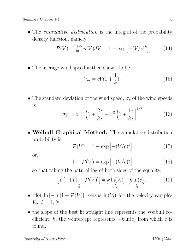
• The cumulative distribution is the integral of the probability

density function, namely

P(V ) =∫ ∞0p(V )dV = 1− exp

[−(V/c)k

](14)

• The average wind speed is then shown to be

Vm = cΓ(1 +1

k). (15)

• The standard deviation of the wind speed, σv of the wind speeds

is

σV = c

Γ1 +

2

k

− Γ21 +

1

k

1/2

(16)

•Weibull Graphical Method. The cumulative distribution

probability is

P(V ) = 1− exp[−(V/c)k

](17)

or,

1− P(V ) = exp[−(V/c)k

](18)

so that taking the natural log of both sides of the equality,

ln [− ln[1− P(V )]]︸︷︷︸y

= k ln(Vi)︸︷︷︸Ax

− k ln(c)︸︷︷︸B

. (19)

• Plot ln [− ln[1− P(V )]] versus ln(Vi) for the velocity samples

Vi, i = 1, N

• the slope of the best fit straight line represents the Weibull co-

efficient, k, the y-intercept represents −k ln(c) from which c is

found.



Rayleigh Distribution

• The Rayleigh distribution is a special case of the Weibull distri-

bution in which k = 2. Then

Vm = cΓ (3/2) (20)

or

c = 2Vm√π

(21)

• In terms of the probability functions, substituting c into the

Weibull expressions:

p(V ) =π

2

V

V 2m

exp

−π4

VVm

2 (22)

of which then

P(V ) = 1− exp

−π4

VVm

2 (23)

so that

P(V1 < V < V2) = exp

−π4

V1

Vm

2− exp

−π4

V2

Vm

2 (24)

and

P(V > Vx) = 1−1− exp

−π4

VxVm

2 = exp

−π4

VxVm

2

(25)



Energy Estimation of Wind Regimes

• The ultimate estimate to be made in selecting a site for a wind

turbine or wind farm is the energy that is available in the wind

at the site, namely wind energy density, ED.

• Other parameters of interest are the most frequent wind velocity,

VFmax, and the wind velocity contributing the maximum energy,

VEmax, at the site.

Weibull-based Energy Estimation

• In terms of the Gamma function, the energy density is

ED =ρac

3

2

3

kΓ

3

k

. (26)

• The energy that is available over a period of time, T (e.g. T=24 hrs)

ET = EDT =ρac

3T

2

3

kΓ

3

k

. (27)

• The most frequent wind speed

VFmax = c

k − 1

k

1/k

. (28)

• The wind speed that maximizes the energy

VEmax =c(k + 2)1/k

k1/k(29)



Rayleigh-based Energy Estimation

• Energy density

ED =3

πρaV

3m. (30)

• The energy over a period of time, T ,

ET = TED =3

πTρaV

3m. (31)

• The most frequent wind speed

VFmax =1√2K

=

√√√√√2

πVm. (32)

• The wind speed that maximizes the energy

VEmax =

√√√√√ 2

K= 2

√√√√√2

πVm. (33)



Aerodynamic Performance

Actuator Disk Momentum Theory

Figure 3: Flowfield of a Wind Turbine and Actuator disc.



Figure 4: Variation of the velocity and dynamic pressure through the stream-tube.

(AV )∞ = (AV )d = (AV )w (34)

• Inflow (axial) induction factor, a,

a =V∞ − VdV∞

(35)

• The velocity at the actuator disc, Vd

Vd = V∞ [1− a] . (36)

• The wake velocity, Vw

Vw = V∞ [1− 2a] . (37)



• The the thrust on the rotor

T = 2ρAdV2∞a [1− a] (38)

• The thrust coefficient

CT = T/

1

2ρAdV

2∞

= 4a [1− a] . (39)

• The power extracted from the wind by the actuator disc

P = TVd = 2ρAdV3∞a [1− a]2 . (40)

• The power coefficient, Cp, is defined as the ratio of the power

extracted from the wind, P , and the available power of wind, or

CP = P/

1

2ρAdV

3∞

= 4a [1− a]2 . (41)

• The maximum theoretical power coefficient, CPmax = 0.593, for

which a = 1/3. Called the Betz limit.



• The maximum theoretical power coefficient, CPmax = 0.593, for

which a = 1/3 also holds when wake rotation is included.

• The tangential flow is represented through an angular induction

factor, a′, where

a′ =ω

2Ω(42)

• Define λr as the local speed ratio

λr =Ωr

V∞. (43)

• Define λ is the tip speed ratio

λ =ΩR

V∞. (44)

• A useful relation

a(1− a) = a′λ2r. (45)



Blade Element (BEM) Theory

Figure 5: Example of a wind turbine blade divided into 10 sections for BEM analysis.

• The resultant velocity, VR, is made up of the vector sum of the

wind speed and the rotational speed of the blade section

VR =√

[V∞(1− a)]2 + [Ωr(1 + a′)]2 (46)

• The angle that the resultant velocity makes with respect to the

plane of rotation is the angle

φ = tan−1

V∞(1− a)

Ωr(1 + a′)

. (47)

• The local angle of attack at any radial location on the rotor is

α(r) = φ(r)− [θT (r) + θcp] . (48)



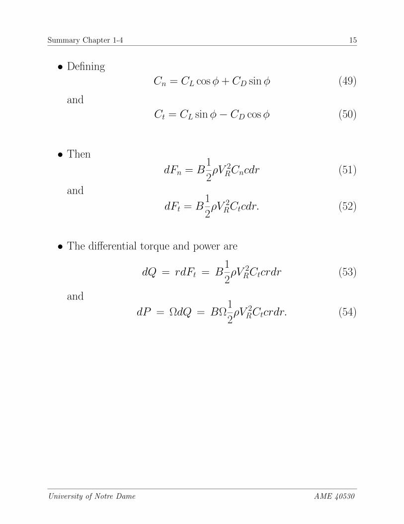
• Defining

Cn = CL cosφ + CD sinφ (49)

and

Ct = CL sinφ− CD cosφ (50)

• Then

dFn = B1

2ρV 2

RCncdr (51)

and

dFt = B1

2ρV 2

RCtcdr. (52)

• The differential torque and power are

dQ = rdFt = B1

2ρV 2

RCtcrdr (53)

and

dP = ΩdQ = BΩ1

2ρV 2

RCtcrdr. (54)



• Defining a new parameter

σr =Bc

2πr(55)

then

a =1

4 sin2 φσrCn

+ 1. (56)

and

a′ =1

4 sinφ cosφσrCt

− 1. (57)



BEM Theory Tip Loss

• Tip loss factor

F =2

πcos−1

(e−f

)(58)

where

f =B

2

R− rr sinφ

(59)

• The tip loss factor is introduced into the differential thrust as

dT = 2FρV 2∞a(1− a)2πrdr. (60)

and

dQ = 2Fa′(1− a)ρV∞Ωr2(2πrdr). (61)


atmospheric boundary layer - university of notre...

Documents