atmospheric radiative transfer - ua hydrology and ... · atmo 551a intro to optical depth fall 2010...

ATMO 551a Intro to Optical Depth Fall 2010

1 Kursinski 11/24/10

Atmospheric Radiative Transfer

We need to understand how energy is transferred via radiation within the atmosphere. We introduce the concept of optical depth. We will further show that the light moves approximately a distance equal to an optical depth of unity and we will use that to gain more insight into how to think about radiative transfer. We will also use the Earth as an example to show that optically thick atmospheres are convectively unstable. Note that this discussion is in terms of 1D radiative transfer in the vertical direction which is the direction of 1st order relevance to radiative transfer.

Suppose we are looking down at the atmosphere observing the IR radiation emerging from

the atmosphere. For now, we assume no scattering effects. We use Beer’s Law where

€

dI = −I α dz = −I dτ (0)

where I is intensity in watts/m2, α is the extinction coefficient in units of inverse length, z is path length and τ is known as optical depth. α‘s units of inverse length represent how much attenuation there is per unit length.

From Kirchhoff’s law, a good absorber is a good emitter and a poor absorber is a poor emitter (at the wavelengths where it is a poor absorber). We need the equation for emission to understand how the atmosphere cools itself by emitting IR radiation.

It can be shown that the radiation emission from a height interval with thickness, dz, is

dIv = α(v,z) B(v,T) dz (1)

where B(v,T) is the Planck function (the black body curve) and α is the absorption coefficient in units of inverse length.

This emitted radiation is then attenuated by absorption as it passes through the atmosphere. The radiance from that height interval that leaves the atmosphere is therefore

€

dIe υ,z( ) = α υ,z( )B υ,T( )e−τ υ ,z( )dz = dIυe−τ υ ,z( ) (2)

where τ is the optical thickness above altitude of emission, z, where

(3)

Note that τ is defined here such that τ = 0 at the top of the atmosphere. So the spectral intensity of the atmosphere is

€

Ba v( ) = α v,z( )0

∞

∫ B v,T(z)[ ]e−τ v,z( )dz (4)

There is also a contribution from the emission from the surface, Bs. So the total emission seen from above the Earth is

Βt(v) = Βa(v) + Bs

€

e−τm v,z( ) (5)

where τm is the total optical depth of the atmosphere from the surface to space:

(6)



There is a variable, X, called the transmission through the atmosphere that is equal to

€

e−τ v,z( ) . The vertical derivative of X is then

€

dXdz

=de−τ υ ,z( )

dz= −e−τ υ ,z( ) dτ

dz= α υ,z( ) e−τ υ ,z( ) (7)

The last sign change comes from the derivative of (3) w.r.t. z. This allows Ba in (4) to be written somewhat more compactly as

€

Ba v( ) = B v,T(z)[ ] dX v,z( )dz0

∞

∫ dz (8)

The peak altitude of emission

Now lets look at the vertical level where the most emission comes from. Assuming

€

B v,T(z)[ ] does not vary too dramatically with altitude, then the answer is the answer to the

question: at what altitude does

€

dX v,z( )dz

reach a maximum?

€

ddzdXdz

= 0 =ddz

α υ,z( ) e−τ υ ,z( )[ ] =ddzα υ,z( ) − α υ,z( ) d

dzτ υ,z( )

⎡

⎣ ⎢ ⎤

⎦ ⎥ e−τ υ ,z( )

€

0 =ddzα υ,z( ) + α 2 υ,z( )

⎡

⎣ ⎢ ⎤

⎦ ⎥ e−τ υ ,z( )

€

ddzα υ,z( ) = − α 2 υ,z( ) (9)

Now, we need to remember get an equation for α is to use an approximate form for it to understand the implications of (9). (In the Hygrometer notes: )

€

α = kv,υ = Sv,υ f υ −υ 0( ) (10)

where S is the line strength of the absorption line, f represents the shape of the absorption line,

€

υ is the frequency of the measurement and

€

υ 0 is the line center of the absorption line. The line shape is due to a combination of Doppler and pressure broadening. The line strength is given as

€

Sv,υ = nmgi exp −Ei kT( )

ZCij

c1− e−hυ ij / kT[ ] = n nm

ngi exp −Ei kT( )

ZCij

c1− e−hυ ij / kT[ ] (11)

where n is the total number density of the bulk gas = P/kBT and nm/n is the volume mixing ratio of constituent m of the gas, Ei is the energy of the transition between two energy levels (i and j) of the molecule,

€

υ 0=

€

υ ij , g is the number of states with Z is the partition function which is

€

gi exp −Ei kBT( )i∑ which is the sum of population of all of the available states at a particular

temperature, T, and Cij is an electromagnetic coupling factor for this particular energy transition.

The main point right now is that S is proportional to the number density of the absorber, n. This in general falls off exponentially with altitude.

So we plug a simple exponential form in for α(z) = α0 e-z/H into (9) which results in



€

−α0e

−zmax / H

H= − α0

2 e−2zmax / H

€

ezmax / H = α0 H

€

zmaxH

= ln α0 H[ ]

€

zmax = H ln α0 H[ ] (12)

Plug (12) into (3) we find the value of τ at zmax at which

€

dXdz

reaches a maximum value

€

τ v,zmax( ) = α0e−ξ / H

zmax

∞

∫ dζ = −α0He−ξ / H

zmax

∞= α0He

−zmax / H = α0H exp −H ln α0 H[ ]

H

⎛

⎝ ⎜ ⎜

⎞

⎠ ⎟ ⎟

€

τ v,zmax( ) = α0H exp −ln α0 H[ ]( ) = α0H1

α0 H=1 (13)

So indeed

€

dXdz

reaches a maximum value around τ = 1.

What is the (spectrally averaged) IR optical depth of Earth’s atmosphere?



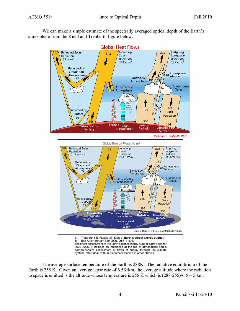
We can make a simple estimate of the spectrally averaged optical depth of the Earth’s atmosphere from the Kiehl and Trenberth figure below.

Author's personal copy

An imperative for climate change planning: tracking Earth’s global energy Trenberth 21

Figure 2

The global annual mean Earth’s energy budget for the March 2000–May 2004 period in W m!2. The broad arrows indicate the schematic flow of energyin proportion to their importance. From Trenberth et al. [6""].

Figure 3

Global sea level since August 1992. The TOPEX/Poseidon satellite mission provided observations of sea level change from 1992 until 2005. Jason-1,launched in late 2001 continues this record by providing an estimate of global mean sea level every 10 days with an uncertainty of 3–4 mm. Theseasonal cycle has been removed and an atmospheric pressure correction has been applied. http://sealevel.colorado.edu/ courtesy Steve Nerem(reproduced with permission).

www.sciencedirect.com Current Opinion in Environmental Sustainability 2009, 1:19–27

Author's personal copy

or La Nina events, and those that are intrinsically part ofclimate change, whether a slow adjustment or trend, suchas the warming of land surface temperatures relative tothe ocean and changes in precipitation characteristics.Regional climate change also depends greatly on patternsor modes of variability being sustained and thus relies oninertia in the climate system that resides mostly in theoceans and ice components of the climate system. Aclimate information system that firstly determines whatis taking place and then establishes why is better able toprovide a sound basis for predictions and which cananswer important questions such as ‘Has global warmingreally slowed or not?’ Decisions are being made thatdepend on improved information about how and whyour climate system is varying and changing, and theimplications.

AcknowledgementsThis research is partially sponsored by the NOAA CLIVAR and CCDDprograms under grants NA06OAR4310145 and NA07OAR4310051.

References and recommended readingPapers of particular interest, published within the annual period ofreview, have been highlighted as:

! of special interest!! of outstanding interest

1. Easterling DR, Wehner MF: Is the climate warming or cooling?Geophys Res Lett 2009, 36:L08706 doi: 10.1029/2009GL037810.

2.!

Solomon S, Qin , Manning M, Chen , Marquis M, Averyt KB, TignorM, Miller HL (Eds): IPCC: Climate Change 2007: The PhysicalScience Basis. Cambridge Univ Press; 2007:996 pp..

This is the Intergovernmental Panel on Climate Change Fourth Assess-ment Report (AR4) that provides a comprehensive review of climatechange up to about 2005.

3. Kopp G, Lawrence G, Rottman G: The total irradiance monitor(TIM): science results. Solar Phys 2005, 230:129-140.

4. Frohlich C: Solar irradiance variability since 1978—revision ofthe PMOD composite during solar cycle 21. Space Sci Rev2006, 125(1–4):53-65.

5. Duffy P, Santer B, Wigley T: Solar variability does not explainlate-20th-century warming. Phys Today (January)2009. 48-49,S-0031-9228-0901-230-7.

6.!!

Trenberth KE, Fasullo JT, Kiehl J: Earth’s global energy budget.Bull Amer Meteor Soc 2009, 90:311-323.

The latest assessment of the Earth’s global energy budget is provided for2000–2005. It includes an imbalance at the top of atmosphere and acomprehensive assessment of flows of energy through the climatesystem, often dealt with in piecemeal fashion in other studies.

7.!

Fasullo JT, Trenberth KE: The annual cycle of the energybudget: Pt I. Global mean and land-ocean exchanges. J Clim2008, 21:2297-2313.

This study provides the main basis for reference [6!!] at the top ofatmosphere, for the global oceans and global land, and provides thelatest estimates of global energy balance as a function of time of year.

8. Trenberth KE, Smith L, Qian T, Dai A, Fasullo J: Estimates of theglobal water budget and its annual cycle using observationaland model data. J Hydrometeor 2007, 8:758-769.

9. Kiehl J: On the observed near cancellation between longwaveand shortwave cloud forcing in tropical regions. J Clim 1994,7:559-565.

10. Walsh JE, Chapman WL, Portis DH: Arctic cloud fraction andradiative fluxes in atmospheric reanalyses. J Clim, 2009,22:2316–2324 doi:10.1175/2008JCLI2213.1.

11. Cazenave A, Dominh K, Guinehut S, Berthier E, Llovel W,Ramillien G, Ablain M, Larnicol G: Sea level budget over 2003–2008: a reevaluation from GRACE space gravimetry satellitealtimetry and Argo. Global Planet Change 2009, 65:83-88doi:10:1-16/j.gloplacha.2008.10.004.

12. Trenberth KE, Fasullo JT:Changes in the flow of energy throughthe climate system. Meteorologische Zeitschrift, 2009, in press.

13.!

Wouters B, Chambers D, Schrama EJO:GRACE observes small-scale mass loss in Greenland. Geophys Res Lett 2008,35:L20501 doi: 10.1029/2008GL034816.

This study is one of several detailing recent (2003–2007) acceleratedmelting of Greenland and is convincing in its use and reconciliation of botha model and gravity observations from space.

14. Kohl A, Stammer D: Decadal sea level changes in the 50-YearGECCO ocean synthesis. J Clim 2008, 21:1876-1890.

15. Loeb NG, Wielicki BA, Doelling DR, Smith GL, Keyes DF, Kato S,Manalo-Smith N,Wong T:Towardsoptimal closure of theEarth’sTop-of-Atmosphere radiation budget. J Clim 2009, 22:748-766.

16. Karl TR, Trenberth KE: Modern global climate change. Science2003, 302:1719-1723.

17. Flanner MG: Integrating anthropogenic heat flux with globalclimatemodels.Geophys Res Lett 2009, 36:L02801 doi: 10.1029/2008GL036465.

18. Trenberth KE, Stepaniak DP: The flow of energy through theEarth’s climate system. Quart J Roy Meteor Soc 2004,130:2677-2701.

19. Wylie D, Jackson DL, Menzel WP, Bates JJ: Trends in globalcloud cover in two decades of HIRS observations. J Clim 2005,18:3021-3031.

20. Kim D, Ramanathan V: Solar radiation and radiative forcing dueto aerosols. J Geophys Res 2008, 113:D02203 doi: 10.1029/2007JD008434.

21. Remer LA, Kleidman RG, Levy RC, Kaufman YJ, Tanre D,Mattoo S, Martins JV, Ichoku C, Koren I, Yu H, Holben BN: Globalaerosol climatology from the MODIS satellite sensors. JGeophys Res 2008, 113:D14S07 doi: 10.1029/2007JD009661.

22. Trenberth KE, Dai A: Effects of Mount Pinatubo volcaniceruption on the hydrological cycle as an analog ofgeoengineering. Geophys Res Lett 2007, 34:L15702 doi:10.1029/2007GL030524.

23. Beltrami H, Smerdon JE, Pollack HN, Huang S: Continental heatgain in the global climate system. Geophys Res Lett 2002,29(8):1167 doi: 10.1029/2001GL014310.

24.!

Rignot E, Bamber JL, van den Broeke MR, Davis C, Li Y, van deBerg WJ, van Meijgaard E: Recent Antarctic ice mass loss fromradar interferometry and regional climate modeling. NatGeosci 2008, 1:106-110 doi: 10.1038/ngeo102.

This study details the accelerated melt of Antarctica in recent years usinga comprehensive approach that builds confidence in the findings.

25. Kay JE, L’Ecuyer T, Gettelman A, Stephens G, O’Dell C: Thecontribution of cloud and radiation anomalies to the 2007Arctic sea ice extent minimum. Geophys Res Lett 2008,35:L08503 doi: 10.1029/2008GL033451.

26. Trenberth KE, Fasullo J: An observational estimate of oceanenergy divergence. J Phys Oceanogr 2008, 38:984-999.

27. Gouretski V, Koltermann KP: How much is the ocean reallywarming? Geophys Res Lett 2007, 34:L01610 doi: 10.1029/2006GL027834.

28. Wijffels SE, Willis J, Domingues CM, Barker P, White NJ, Gronell A,Ridgeway K, Church JA: Changing expendableBathythermograph fall-rates and their impact on estimates ofthermosteric sea level rise. J Clim 2008, 21:5657-5672.

29. Jevrejeva S, Moore JC, Grinsted A: Relative importance of massand volume changes to global sea level rise. J Geophys Res2008, 113:D08105 doi: 10.1029/2007JD009208.

30. Lyman JM, Johnson GC: Estimating annual global upper-oceanheat content anomalies despite irregular in situ oceansampling. J Clim 2008, 21:5629-5641.

26 Inaugural issues

Current Opinion in Environmental Sustainability 2009, 1:19–27 www.sciencedirect.com

The average surface temperature of the Earth is 288K. The radiative equilibrium of the Earth is 255 K. Given an average lapse rate of 6.5K/km, the average altitude where the radiation to space is emitted is the altitude whose temperature is 255 K which is (288-255)/6.5 = 5 km.



Since this is the average altitude where thermal emission from Earth is leaving into space, this must be the altitude where the spectrally averaged optical depth (measured from the top of the atmosphere) is about 1.

The downwelling IR into Earth’s surface is 324 W/m2. We set this equal to σT4 to find the temperature level in the atmosphere where this radiation is coming from. The answer is 275K. Again, using an average surface temperature of 288 K and an average lapse rate of 6.5 K/km, we see that the altitude of this downwelling radiation is 2 km. Now when measured from the surface, this altitude corresponds to an optical depth of 1.

So we know that from space to an altitude of 5 km is approximately a spectrally averaged IR optical depth of 1 and from the surface to an altitude of 2 km, the change in IR optical depth is about 1. What is the spectrally averaged optical depth change between 2 and 5 km?

The pressure at 5 km is about 550 mb. So the amount of atmospheric mass above 5 km is about 55% of the atmosphere. The pressure change between the surface and 2 km is about 200 mb (=1000mb - 800mb) or about 20% of the atmosphere. The pressure change between 2 and 5 km is about 800 mb - 550 mb = 250 mb. So, based on this relation between optical depth and mass, my guess is the spectrally averaged IR optical depth across this interval is slightly less than unity. So the spectrally averaged IR optical depth of the entire atmosphere is about 3.

The reason the gradient of optical depth w.r.t. to atmospheric mass increases at higher pressure and temperature is a combination of increased water vapor at warmer temperatures and the fact that at higher pressure the spectral interval between the absorption lines fills in as the lines broaden.

Comment on Venus, Earth and Mars: Venus has an enormous CO2 atmosphere. Bill Nye says because of the massive amount of CO2 Venus has an enormous greenhouse effect. Mars has more CO2 in the atmosphere than Earth. Does it have a big greenhouse effect? No. Why not? Simple layered radiative transfer model for optically thick atmospheres.

Consider an atmosphere divided into vertically stratified layers. The vertical thickness of each layer is defined to be such that the change in the spectrally averaged optical thickness across the depth of the layer is unity. We can then write the radiative transfer equilibrium solution in the following approximate way. Note that we are assuming convection and diffusional energy transfer are negligible.

Starting from the top, at optical depth 1 we have radiative equilibrium with no IR coming in from the top, radiation coming in and being absorbed from the layer below and the layer itself radiating both up and down. We can write this as

€

2σT14 =σT2

4



For the second layer, the energy into the layer is coming from the layers immediately above and below the 2nd layer. The layer itself again emits both up and down. So the radiative equilibrium condition is

€

2σT24 =σT1

4 +σT34

This generalizes to

€

2σTi4 =σTi−1

4 +σT1+14

At the surface we have

€

σTn+14 =σTn

4 + Fsol

Where Tn+1 is the surface temperature under n atmospheric layers and Fsol is the solar flux absorbed by the surface. Clearly the temperature fo the top layer must be the radiative equilibrium temperature. The temperature of the second layer is 21/4 Teq. The temperature of the third layer is

€

T3 = 2T24 −T1

4[ ]1/ 4 = 2*2T14 −T1

4[ ]1/ 4 = 3T14[ ]1/ 4 = 31/ 4T1

The general solution to the vertical temperature structure is Ti = i1/4 Teq.

Now we can compare this optically thick radiative-only atmospheric temperature structure with that of Earth. Temperature T1 is 255K. Temperature T2 is 303K and T3 =336. As the table shows, given the altitudes of the optical depths of 1, 2 and 3 levels in the atmosphere, we can determine the lapse rates when the vertical energy exchange is via radiative only. Optical Depth T (K) Altitude (km) dT/dz (K/km)

1 255 5 -16.1 2 303 2 -16.2 3 336 0

The issue is that the temperature gradients are larger than the dry adiabat. So when the atmosphere move to get hot enough to radiatively transfer the absorbed solar energy back out to space, it becomes convectively unstable and begins to transfer some of the energy upward via convection. This shows that a purely radiative atmosphere is convectively unstable and is never actually achieved for atmospheres where the (spectrally averaged) IR optical depth exceeds unity. So convection kicks in and transfers energy vertically and we have a radiative-convective troposphere. This is why the tropopause on planets and moons with major atmospheres is a bit above the τ =1 level in the atmosphere.

atmospheric radiative transfer - ua hydrology and ... · atmo 551a intro to optical depth fall 2010...

Documents