monte carlo simulation of radiative transfer in...
TRANSCRIPT

6
Monte Carlo Simulation of Radiative Transfer in Atmospheric Environments for Problems
Arising from Remote Sensing Measurements
Margherita Premuda Institute of Atmospheric Sciences and Climate, National Research Council (ISAC-CNR),
via Gobetti 101, 40129 Bologna, Italy
1. Introduction
The way in which solar radiation distributes itself in the atmosphere and on the ground is well known. It is beyond the scope of this book and the reader can refer to more specific references (Kondratyev, 1969; Goody & Yung, 1995; Liou, 1998) for more detail. Solar radiation, essentially in the visible-ultraviolet frequency range, and infrared radiation, emitted by the terrestrial surface, are the prevailing energy sources for general atmospheric circulation. They are thus particularly important for meteorological and climatic studies. It would therefore be of great interest, for instance, to be able to calculate the influence of the presence of ozone and trace gases, water vapour and clouds, and various aerosols on radiative transfer and global thermal energy in the atmosphere or in particular regions of it. These considerations naturally lead to the analysis of radiative transfer in the terrestrial atmosphere. This can be done using an atmospheric radiative transfer model (RTM) which also includes the possibility of single and multiple scattering events. Numerical and analytical methods can be used to solve a radiative transfer equation (Stamnes et al., 1988; Lenoble, 1977; Fouquart et al., 1980). A Monte Carlo approach is particularly suitable when multiple scattering significantly affects the results or where marked anisotropy of scattering and complex geometrical configurations are involved. The interest in such problems has increased through recently developed techniques related to remote sensing observations (satellite-based, ground-based or airborne) of the Earth's surface and atmosphere, involving the use of spectral radiation dispersion systems (mainly radiometers, spectrometers and interferometers) and active systems (principally RADAR, LIDAR and SODAR) Among these various techniques, DOAS (Differential Optical Absorption Spectroscopy) and LIDAR (Light Detection And Ranging) investigations on the presence of particular atmospheric constituents or of atmospheric phenomena such as clouds, fog, rain, etc., are of special interest. With reference to surface remote sensing observations, for instance, the effects of atmospheric absorption and scattering constitute a noise element, which has to be evaluated by calculations. Simulation of both LIDAR and DOAS systems deals with radiation in the UV/visible
spectral range. For simulation purposes, a LIDAR system can be schematized as a pulsed
www.intechopen.com
Applications of Monte Carlo Method in Science and Engineering
96
laser “disk” source of monochromatic radiation and a “disk” receiver (the “disk”
schematization will be explained later), respectively with small emitting and receiving
angles, i.e., with a narrow field of view (FOV). By means of Monte Carlo simulations, it is
possible to analyze the time and spatial distributions of the backscattering radiation due to
various atmospheric components. The equation for a LIDAR backscattering signal as well as
further considerations relating to Monte Carlo simulations has been published (Pace et al.,
2003; Coletti & Fiocco, 1980).
DOAS (Noxon, 1975; Platt et al., 1979; Platt & Perner, 1980; Roscoe et al., 1999) is an
established remote sensing technique which identifies and quantifies the trace gases in the
atmosphere taking advantage of their absorption structures in the near UV and visible
wavelengths of the solar spectrum (passive DOAS). For simulation purposes, DOAS systems
can be represented by a disk detector of solar radiation, with a relatively small diameter and
a narrow FOV.
For our purposes, the atmosphere can be considered to consist of two different kinds of
components: molecular (gases) and non-molecular (aerosol), which interact with radiation in
different ways. For both components, a knowledge of their interaction coefficients and of the
angular distributions of the scattered radiation (phase functions) is required. Appropriate
average values of interaction coefficients for suitable altitude subdivisions have to be
computed by taking into account the height variation of their density. Regarding molecular
components, both continuum and line absorption are considered. The former accounts for
reciprocal interactions between molecules of the same or other species whereas line
molecular absorption is connected to rotational and rotational-vibrational transition
frequencies, characteristic of each kind of molecule. Using theoretical models it is possible to
find analytical expressions for line absorption coefficients as functions of such frequencies
(Clough, et al., 1981; Kneizys et al., 1983a; Kneizys et al., 1984; Kondratyev, 1969). For
radiation scattering by molecular components, the well-known expression of scattering
coefficients and phase functions arising from Rayleigh theory can be adopted (Kondratyev,
1969). For non-molecular atmospheric components, scattering coefficients and phase
functions can be derived from the Mie theory (Kondratyev, 1969; Lenoble, 1977) for particles
whose dimensions are comparable to the radiation wavelength. Besides the exact Mie phase
functions, several approximate formulae are available, the most suitable being the Henyey-
Greenstein approximation (Kondratyev, 1969; Lenoble, 1977), based on a knowledge of the
asymmetry factor g (average cosine of the scattering angle). As can be seen in Figure 1
(Tomasi & Paccagnella, 1986), the Mie phase functions may show marked anisotropy.
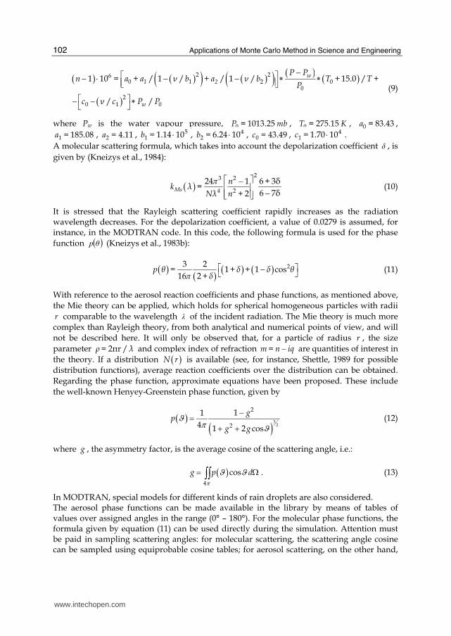
In the simulation of radiation transport through the atmosphere the phenomenon of
refraction has to be taken into account as a consequence of different refractive index values
between contiguous geometrical shells. This phenomenon can be remarkable, for instance,
in the case of vertical view detectors receiving solar radiation at solar zenith angles near to
or greater than 90° (horizon) as can be seen in Figure 2, where a plot of a sun ray, obtained
using the MOCRA (MOnte Carlo Radiance Analysis) code for a 93° solar zenith angle
(Premuda et al., 2009) is shown. This phenomenon is taken into account according to Snell’s
refraction law sin sini r r in n ϑ ϑ= , where in and rn are the average refractive indices of
the two contiguous regions involved and iϑ and rϑ are the incident and refracted angles
with respect to the normal to the boundary surface, respectively. It should be noted that
total reflection occurs for incident angles greater than a critical value.
www.intechopen.com

Monte Carlo Simulation of Radiative Transfer in Atmospheric Environments for Problems Arising from Remote Sensing Measurements
97
Fig. 1. Phase function for spherical particles. Reproduced by courtesy of SIF (Italian Physical Society) (Tomasi & Paccagnella, 1986).
-3,00E+01
-2,50E+01
-2,00E+01
-1,50E+01
-1,00E+01
-5,00E+00
0,00E+00
300,00 350,00 400,00 450,00 500,00 550,00 600,00 650,00 700,00 750,00 800,00
z (
Km
)
x (Km)
Z-Refr.
Z-Lin
EARTH
Fig. 2. Plot of refraction of a sun ray obtained using the MOCRA code for a 93° solar zenith angle. The refracted ray (dark blue) hits the Earth's surface (brown), whereas the linear ray, without refraction (magenta), would reach the vertical above the observer.
At ground level, the albedo phenomenon usually has to be taken into account according to appropriate surface albedo coefficients. Towards this end, the Lambert reflection law is frequently adopted, which assumes a cosine distribution law for the reflected radiation with
www.intechopen.com

Applications of Monte Carlo Method in Science and Engineering
98
respect to the normal to the ground surface. The values of the albedo coefficient may significantly depend upon the radiation wavelength and on the surface characteristics (snow cover, foliage, bare soil, etc.). Bidirectional reflectance distribution functions (BRDF), particularly useful for analyzing ground reflectance properties, may also be considered, as they take into account the solar zenith angle, the observer line of sight and the azimuth between the solar and observer directions. A theoretical model of the BRDF compared to experimental observations is available (Walthall et al., 1985). A Monte Carlo simulation has also been used (Richtsmeier & Sundberg, 2009). Very accurate molecular and non-molecular models are adopted in the radiance-transmittance MODTRAN codes (Berk et al., 1989; Kneizys et al., 1996; Acharya et al., 1998; Berk et al., 1999), where physical phenomena involving radiation in the infrared-ultraviolet spectral range are analyzed in detail. They are used widely by the remote-sensing community to model spectral absorption, transmission, emission and scattering characteristics of the atmosphere. Through a knowledge of interaction coefficients and phase functions, it is possible to set up sequences of discrete and continuous probability distribution functions (p.d.f.) which allow Monte Carlo photon-history tracking. Monte Carlo simulations related to LIDAR and DOAS systems will be described below, together with proper variance reducing techniques. A variety of Monte Carlo applications have been described (Marseguerra & Zio, 2002).
2. General features of Monte Carlo radiative transfer simulations in atmospheric environments
An appropriate description of a numerical or statistical simulation of radiation transport in an atmospheric environment requires a theoretical equation which governs the transport phenomenon to be stated and the physical and geometrical properties of the environment defined. To this end, in what follows, a simplified form of the integral transport equation will be given together with a possible environmental representation suitable for the simulation process, which will be subsequently described in its general fundamental lines.
2.1 Integral radiative transfer equation and Monte Carlo simulation
To analytically describe, in its photonic representation, radiation transport in atmospheric environments for time independent problems, the following integral form of the Radiative Transfer Equation (RTE) can be written for the specific intensity of radiation ( )I r,Ω defined as the photonic distribution function times ch┥ , where c is the velocity of light in a vacuum, h Planck’s constant and ν the radiation frequency
( ) ( ) ( )
( ) ( )0
0 0
, , exp
, exp
s
s
r r
s
r r s
I r r ds k r s
ds Q r s ds k r s
−
′−
⎡ ⎤′′ ′′Ω = Γ Ω − − Ω +⎢ ⎥⎣ ⎦⎡ ⎤′ ′ ′′ ′′+ − Ω Ω − − Ω⎢ ⎥⎣ ⎦
∫∫ ∫
(1)
where k is the total extinction coefficient, sum of the scattering sk and the absorption ak coefficients. Q is the source density for emission and scattering defined as
( ) ( ) ( ) ( )4
, , ,sQ r S r d k r I rπ ′ ′ ′Ω = + Ω Ω ⋅Ω Ω∫ . (2)
www.intechopen.com

Monte Carlo Simulation of Radiative Transfer in Atmospheric Environments for Problems Arising from Remote Sensing Measurements
99
where ( )sポ r ,Ω is the source radiation specific intensity. The ( )S r term in equation (2)
represents an internal radiation source.
As can be seen, the specific intensity of radiation in direction Ω at point r is determined by
the sum of two contributions: the first is the direct source contribution, due to the source
specific intensity of radiation starting at point rs and the second accounts for emission and
scattering of the beam radiation coming from each element 'ds of the path from sr to r
along the Ω direction. Both contributions at point r are exponentially attenuated as a
consequence of absorption and scattering collisions. It should be noted that in solar radiance
analysis the first contribution accounts for the irradiance and the second for single and
multiple scattering. The integral form of the transport equation is suitably solved by means of numerical or
Monte Carlo simulations (Marseguerra & Zio, 2002). It can be obtained directly from the
more general integro-differential radiative transfer equation (Spiga et al., 1992; Premuda &
Palestini, 1982; Premuda, 1994).
The attenuating exponentials are the same used to evaluate path lengths between collisions
in Monte Carlo simulations. The length relevant to exponential attenuation of both
contributions is the optical depth, defined as follows:
( ) ( )0
,sr r
sr r ds k r sτ − ′′ ′′= − Ω∫ . (3)
In the standard “forward” Monte Carlo simulation, histories of photons emitted from the radiation source are followed until they hit the detector or disappear from the system as a consequence of leakage or absorption. Problems in this simulation procedure inevitably arise when small detectors with narrow FOVs are considered in the presence of an external broad source, due to the very low probability of a photon reaching the detector. To overcome this kind of problem, a “backward” Monte Carlo simulation is usually performed, taking into account that the linearity of the transport Boltzmann equation and the reciprocity relationship between the Green function G(P → Pd) and its adjoint G*(Pd → P) make it possible to write for the flux Φ(Pd)::
( ) ( ) ( ) ( ) ( )dPPSPPGdPPSPPGP ddd →=→=Φ ∫∫ *
(4)
in which the source S(P) is always evaluated at the source point P (a detailed analysis of the Monte Carlo simulation of the adjoint transport Boltzmann equation is available (De Matteis & Simonini, 1978a; De Matteis & Simonini, 1978b)). In the case of solar sources, each photon history is therefore traced through the atmosphere as being generated by the detector according to its line of sight direction, taking into account the phase function for the angle which leads from a collision point Pc to the source point P on the external atmospheric boundary along the solar radiation direction. A backward simulation description for radiation transport in the atmosphere, where polarization effects are also taken into account, is available (Collins et al., 1972). In atmospheric radiative transfer simulations, the backward scheme is even more suitable, because in photon interactions with atmospheric constituents energy changes do not occur. A forward Monte Carlo radiative transfer simulation for photon tracing in three-dimensional cloudy atmospheres is foreseen in the Mystic code (Mayer & Kylling, 2000). Topography and an inhomogeneous surface albedo are considered.
www.intechopen.com

Applications of Monte Carlo Method in Science and Engineering
100
2.2 The atmospheric environment and photon history tracking
For a radiation of assigned wavelength, the photonic interpretation allows the application to
radiative transfer of simulation techniques usually adopted for particle transport in assigned
materials. Starting from the source, trajectories of individual photons are followed,
according to the physical and geometrical properties of the environment of interest and
taking into account the discrete and continuous probability distribution functions belonging
to possible events for the photon.
A synthetic description of the essential characteristics of the atmospheric environment
required for the simulation process and of the standard “forward” history tracking is given
below.
a) The atmospheric environment
Regarding the physical properties, as mentioned previously, reaction coefficients and phase
functions for both molecular and aerosol particles are required. A knowledge of these
parameters, together with refractive indices, which characterize each kind of atmosphere,
can be profitably used to build a library data set, then used as the source of the fundamental
physical and geometrical values needed for the Monte Carlo simulation. In analyzing
radiative transfer in atmospheric environments, it can be crucial to verify the effects on
radiation transport of perturbations in some atmospheric constituents (e.g. small variations
in ozone or carbon dioxide concentrations). In Monte Carlo simulations it is possible to
evaluate these effects by considering simultaneously reference and perturbed environments.
This can be done by tracing the photon histories in the reference environment, taking into
account the perturbations using appropriate weighting functions. This simulation tool
makes it possible to evaluate small effects which could be masked by statistical errors when
using separate calculations. This is possible, for instance, in the MOCRA code where several
perturbed environments can be considered simultaneously.
In radiation transport simulations in atmospheric environments, great advantage can be
gained by proper representation of general 3D spherical multi-region geometries. The
atmosphere can, for instance, be subdivided into cones, spherical shells and azimuthal half
planes, obtaining very detailed geometrical descriptions of the various surface and
atmospheric regions (Cupini et al., 2005). This allows one to take into account various
ground altitudes and atmospheric profiles for each region, thus allowing for soil orography
and latitudinal and longitudinal variations in the composition of the atmosphere. This is
also possible with MOCRA and has been used to simulate the presence of an obstacle in
horizontal passive DOAS measurements (Premuda et al., 2009).
When several kinds of atmosphere have to be simultaneously taken into account in the same
calculation, as may occur, for instance, in general 3-D geometries, the data belonging to each
of them must obviously be available in the library. The appropriate build-up and treatment
of the physical and geometrical library data can make it possible, for instance, to foresee
effects due to the injection of special aerosols (e.g., fumes) in a given atmospheric region
with already assigned aerosols.
In the following Km are the units of length and, consequently, Km-1 are reaction coefficient
units. As already pointed out, reaction coefficients, given by the product of the density and
the proper particle reaction “cross section”, will depend on the particle density behaviour
along the vertical z-axis starting from the ground altitude, so that average values are to be
computed in Monte Carlo simulations. To this end, the total assumed atmospheric height
www.intechopen.com

Monte Carlo Simulation of Radiative Transfer in Atmospheric Environments for Problems Arising from Remote Sensing Measurements
101
range (z0, zmax) can be subdivided into an assigned number NL of conveniently chosen
geometrical layers. With reference to molecular particles, if one assumes an exponential
behaviour of the density spatial distribution within each layer, depending upon the pressure
and temperature profiles, one obtains, for the j-th layer:
( ) ( ) ( ) ( ) ( )1 1/ln /exp / j j+ j j j+j j j H = z z ┩ ┩┩ z = ┩ z z z H ;⎡ ⎤ −− −⎣ ⎦ (5)
The average density value j
┩ within the layer will be given by:
( ) ( )1
1j
j
z
j jj zz dz z zρ ρ+ += −∫ (6)
i.e.:
( ) ( )1 1/ln /j j+ j j+j┩ = ┩ ┩ ┩ ┩− (7)
If, for numerical reasons, this relationship cannot be applied, the value j
┩ can be assumed
to be equal to the arithmetic mean of ┩j and ┩j+1. Similar relationships will hold,
consequently, for the average molecular scattering Ms jk and absorption Ma j
k
coefficients. It can be observed that, although a unique value is usually given for the
scattering coefficient, corresponding to that of air considered as a fictitious molecule with a
molecular weight MAir = 28.964, average absorption coefficients must be assigned for each
molecular species. The average coefficient Ma jk has to be interpreted as the sum over the
average coefficients belonging to each of them.
Analogous considerations can be made for the average aerosol coefficients As jk and
Aa jk for the same layers, and for the refraction indices. It can be seen that very different
kinds of aerosols can be found along the z-axis, from the boundary layer to the high
stratosphere, so that marked discontinuities can occur in the average reaction coefficients
between contiguous layers. For the j-th vertical layer, the following total coefficients can be considered:
M Ms Ma A As Aajj j j j jk = k + k ; k = k + k . (8)
According to eq. (3), the optical depth of the layer will be: j jj┬ = k h . This optical depth
characterizes the layer in the atmospheric environment and gives a measure of the
transparency of the layer to the incident radiation. For the sake of simplicity, in what follows
the brackets will be omitted.
In the photon diffusion process, an essential role is played by molecular Rayleigh scattering,
which affects the distance travelled and the motion direction following a collision. A
theoretical formula for the scattering coefficient Msk which takes into account the
dependence on wavelength ┣, refraction index n and molecular number density N is given
by Kondratyev (Kondratyev, 1969) together with phase function and refraction index
expressions. A refraction index formula for standard air, which takes into account the
wavenumber dependence, is available (Edlén, 1966). In the LOWTRAN-MODTRAN codes
the following formula is adopted (Kneizys et al., 1983b):
www.intechopen.com
Applications of Monte Carlo Method in Science and Engineering
102
( ) ( )( ) ( )( ) ( ) ( )
( )2 26
0 1 2 00
20 1 0
1 10 / 1 / / 1 / 15.0 /
/ /
w1 2
w
P Pn = a + a ┥ b + a ┥ b T + T +
P
c ┥ c P P
−⎡ ⎤− ⋅ − − ∗ ∗⎢ ⎥⎣ ⎦⎡ ⎤− − ∗⎣ ⎦
(9)
where Pw is the water vapour pressure, 0 1013.25P = mb , 0 275.15T = K , 0 83.43a = ,
1 185.08a = , 2 4.11a = , 51 1.14 10b = ⋅ , 4
2 6.24 10b = ⋅ , 0 43.49c = , 41 1.70 10c = ⋅ .
A molecular scattering formula, which takes into account the depolarization coefficient δ , is
given by (Kneizys et al., 1984):
( ) 23 2
2
24 1 6 3δ6 7δ2
Ms 4
┨ n +k ┣ =
N┣ n +
⎡ ⎤−⎢ ⎥ −⎢ ⎥⎣ ⎦ (10)
It is stressed that the Rayleigh scattering coefficient rapidly increases as the radiation wavelength decreases. For the depolarization coefficient, a value of 0.0279 is assumed, for instance, in the MODTRAN code. In this code, the following formula is used for the phase
function ( )θp (Kneizys et al., 1983b):
( ) ( ) ( ) ( ) 23 21 1 cos
16 2p θ = + ├ + ├ θ
┨ + ├⎡ ⎤−⎣ ⎦ (11)
With reference to the aerosol reaction coefficients and phase functions, as mentioned above,
the Mie theory can be applied, which holds for spherical homogeneous particles with radii
r comparable to the wavelength λ of the incident radiation. The Mie theory is much more
complex than Rayleigh theory, from both analytical and numerical points of view, and will
not be described here. It will only be observed that, for a particle of radius r , the size
parameter 2┨r /┩= ┣ and complex index of refraction m = n iq− are quantities of interest in
the theory. If a distribution ( )N r is available (see, for instance, Shettle, 1989 for possible
distribution functions), average reaction coefficients over the distribution can be obtained.
Regarding the phase function, approximate equations have been proposed. These include
the well-known Henyey-Greenstein phase function, given by
( ) ( )32
2
2
11
4 1 2 cos
gp
g gϑ π ϑ
−= + + (12)
where g , the asymmetry factor, is the average cosine of the scattering angle, i.e.:
( )4
cosg p dπ
ϑ ϑ= Ω∫∫ . (13)
In MODTRAN, special models for different kinds of rain droplets are also considered. The aerosol phase functions can be made available in the library by means of tables of values over assigned angles in the range (0° – 180°). For the molecular phase functions, the formula given by equation (11) can be used directly during the simulation. Attention must be paid in sampling scattering angles: for molecular scattering, the scattering angle cosine can be sampled using equiprobable cosine tables; for aerosol scattering, on the other hand,
www.intechopen.com

Monte Carlo Simulation of Radiative Transfer in Atmospheric Environments for Problems Arising from Remote Sensing Measurements
103
such tables are, as a rule, not possible to set up, due to the marked anisotropy in their phase functions (Premuda, 1994).
b) Photon history tracking
Once the physical and geometrical properties of the environments required for the
simulation process have been established, the history tracking can be carried out as usual,
taking into account the peculiarities of the problem to be solved. In this regard, it can be
observed that in the efficiency of the simulation aimed at the evaluation of a given quantity
a crucial role is played by the estimator chosen, which will assume a statistical value i┝ at
the end of i-th history. If N histories have been processed, its average value ┤ :
1
N
ii=
┝┤=
N
∑ (14)
will give the estimate of the quantity of interest. As for the statistical error, this can be
estimated by means of the standard deviation for both the estimator, εσ and the estimate,
┤┫ , through the well-known variance equations 2┝ ┝V = ┫ and 2
┤ ┤V = ┫ :
( )21 ,
1
N
ii V
V VN N
εε με μ
=−
= =−∑
(15)
A quantity used to evaluate the efficiency of the simulation process adopted is given by the so-called Figure of Merit (FOM):
1
2┤
FOM =t┫
(16)
where t is a measure of the computation time. As an example of the various possible
choices of the estimator in the simulation process, one can consider the problem of finding the absorption by a given molecule, for instance ozone, of the radiation at an assigned wavelength in a layer. Two kinds of estimators can be adopted: the first one could be derived from the probability of the radiation being absorbed in a collision within the layer (collision estimator); the second by multiplying the distance travelled by the photon within the layer by the absorption coefficient of the molecule (distance estimator). This latter estimator can be conveniently applied when very few collisions occur within a frequently crossed layer.
To take into account in the simulation process the analytical information available on the
physical events which may occur and to develop tools for enhancing the contribution of the
photon history to the final result, a statistical “weight” w is associated with the travelling
photon, taking an initial value 0w assigned at the beginning of the history. In the solar
radiance analysis, for instance, 0w could be assumed to be equal to the radiation intensity
0I of the solar source. Regarding the photon source, the spatial and angular distributions of
the emitted photons will make it possible to select for each history the starting parameters
needed for the subsequent realization of the chain of possible events undergone by the
photon in a given reference system. For this purpose, the importance must be stressed of the
www.intechopen.com

Applications of Monte Carlo Method in Science and Engineering
104
availability of a proper generator of random numbers uniformly distributed over the
interval (0, 1), usually an arithmetic congruence, which, as much as possible, avoid internal
correlations among the generated numbers (Knuth, 1981; De Matteis & Pagnutti, 1988). It is
well known that discrete ( 1 ...2 3p ,p ,p , ) probability distributions and continuous probability
density functions (p.d.f.), both normalized to 1, have to be handled in the history tracking.
In the first case, it is easy to select the kind of event from the distribution by means of proper
comparisons of a chosen random number r with cumulative probability values ( 1r < p ;
1 2r < p + p ; 1 2 3r < p + p + p ; …). In the second, if ( )f x is the p.d.f. normalized to 1 over the
interval ( )ba, , to obtain a value of x the following equation must be solved for the chosen
random number r :
( )x
a
r = f t dt∫ (17)
From this equation, for instance, a value τ of the optical path travelled by the photon is easily obtained from xe− attenuating exponential function, normalized to 1 over the interval ( )0,∞ . When a direct solution is not available or too expensive, special techniques (such as the so-called “rejection technique”) can be used to obtain values of the variable x obeying the p.d.f of interest. In any case, discrete cumulative probability distribution tables can be obtained by means of analytical or numerical integration for assigned values of the independent x variable:
( ) ( )1,2,...,ix
i aP f t dt i N= =∫ (18)
A value of x can be obtained from eq. (17), by means of proper linear interpolations for the chosen random number r. This is, for instance, the case of the Mie phase function, for which, as previously said, tables of values are assumed to be available for the diffusion angle or, more conveniently, its cosine. Taking into account, as already emphasized, the possible marked anisotropy of this distribution function, tabulating points are assumed to be accurately chosen to avoid improper choice of the scattered photon direction. Regarding the Rayleigh phase function, the same approach can be adopted. In this case, as already indicated, a given number (preferably a power of 2, e.g. 32) of cosine intervals can be derived, by means of interpolations, from the cumulative probability table, corresponding to equal probability intervals. In this way, a fast random access to the cosine table allows one to obtain the diffusion angle. On the basis of the previous considerations, to trace, in its fundamental lines, a photon history, an initial assigned weight 0w = w and a selected starting point and motion direction
must first be assigned, as stated previously. The optical path ( )ln┬ = r− , with r random
number ( r and r−1 have the same distribution) to be travelled is then chosen and the
corresponding distance kτ=d / is computed, being k the reaction coefficient of the starting
layer. If the distance d is exhausted within the layer, a collision takes place. A new weight
for the photon is computed by means of the relation: ( )As Msk + k
w = wk
. According to the
probabilities AsAs
As Ms
kp =
k + k and Ms
MsAs Ms
kp =
k + k the choice between the scattering by an
www.intechopen.com

Monte Carlo Simulation of Radiative Transfer in Atmospheric Environments for Problems Arising from Remote Sensing Measurements
105
aerosol or by a molecule is made. If a collision with an aerosol particle occurs and various kinds of aerosols exist within the layer, each with its proper phase function, with
probabilities: A1sA1s
As
kp =
k, A2s
A2sAs
kp =
k, …, the specific kind of aerosol involved will be
selected. On the basis of the proper diffusion cosine distribution function, a new motion
direction will be chosen and a new path started. If the distance d to be travelled is greater
than the distance from the starting point and the boundary of the layer along the motion direction and a leakage phenomenon from the geometrical system does not occur, the optical path exhausted within the layer will be computed, the remaining one being utilized for the next path in the new layer. If refraction is foreseen, according to the refraction indices
1n and 2n belonging to the two contiguous layers, the new refracted motion direction will
be computed. It must be taken into account that a total reflection will occur if 1 2n > n and,
moreover, the angle of the incident direction on the boundary between the two layers is
greater than the Lθ angle, being 2
1
arcsinL
nθ =n
. If the path to be traced hits the ground
surface and an albedo coefficient α is foreseen, a photon with a weight ww *α= will be
reflected with a motion direction chosen according to the diffusion law ( ) 2cos cos
2┨θ θ
f Ω = =┨
with respect to the normal direction to the ground surface (Lambert law). For termination of the history tracking, various criteria can be adopted in addition to that from the leakage of the photon from the geometrical system. Among them, the following
can be considered. 1) Assigning as input parameter a minimum weight fraction, minw , the
history will end if 0
min
w< w
w. The minimum weight fraction has to be carefully chosen to
avoid expensive calculations giving non-essential contributions to the estimator. A value of 10-5 could be, for instance, adopted in many cases. The sum over the histories of the unprocessed weights will give a measure of the bias introduced. 2) Having assigned a
cutting value cutw , if, after a collision, 0
cut
w< w
w, the photon weight will not change. When
a subsequent collision occurs, with a probability As Mss
k + kp =
k this decides whether
scattering occurs. If this is not the case, the history tracking will end. A cutw value equal to
0.2 could be, for instance, assigned. 3) Analogously to the previous point, if 0
cut
w< w
w a
“russian roulette” game is played: with a probability 0
r
wp =
w that the photon will survive
and the initial weight 0w = w will be restored; with a probability 1 rp− that the photon will
be killed and the photon weight lost. At the end of all the histories processed, the sum of the total weight gained should be statistically equal to the total weight lost. To avoid large
jumps in the weight, which can affect the variance, 0.5cutw = could be a reasonable value to
be assigned. In MOCRA, all three options are available. According to the quantities to be estimated through the simulation process, analytical contributions can conveniently be computed during the history tracking, so as to reduce as
www.intechopen.com

Applications of Monte Carlo Method in Science and Engineering
106
much as possible the variance of the calculation. Regarding, for instance, the molecular absorption in a layer, an example is given by the distance estimator previously described. A further estimate frequently required is given by the leakage from the geometrical system. At
each collision point the optical distance e┬ to the external boundary along the direction of
motion is computed. The escape weight ┬e
ew = w e−
will be the analytical contribution of the
collision point to the searched-for estimate. The total sum of the analytical contributions will give the estimator value for that history. In addition to analytical evaluations during the history tracking, variance reducing techniques can be devised which alter the natural sequence of the events undergone by the photon, locally or over the entire physical and geometrical system, giving rise to more efficient unbiased contributions to the required estimates. The most common is given by the well-known forced collision technique. If the direction of motion from a starting or a collision point does not cross a reflecting boundary, the leakage optical distance e┬ is
computed as previously described. The two possibilities for the photon escaping from the
system with a probability ┬ee
− or colliding within it with a probability 1
┬ee−− , are taken
into account separately. More precisely, a photon with a weight ┬e
ew = w e−
is assumed to
travel within the system and escaping from it, whereas a photon with a weight ( )1┬e
cw = w e−− is assumed to collide. It should be noted that both photons are to be
considered when a distance estimator for the absorption is envisaged. To choose the
collision point, the p.d.f. ( )1
x
┬e
ef x =
e
−−− , normalized to 1 over the interval ( )0, e┬ , will then
be adopted for a photon of weight cw = w . When this technique is applied, the first criterion
among those previously described to end the history tracking has to be used. In this case, as a precaution, a maximum number of collisions per history can be assigned. It must be observed that the forced collision technique is an expensive one and it may cause, moreover, considerable changes in the travelling photon weight which can affect the variance. It should be used when the collisions within a system of small optical thickness are of special interest. In any case, the FOM should be taken into account. Further special variance-reducing techniques will be described within the context of the following LIDAR and DOAS simulation analysis. As previously highlighted, to analyze the effect of environmental perturbations on the final result due to small changes in physical parameters which do not affect the phase functions, a simulation process which takes into account, simultaneously, the unperturbed (reference) environment and the perturbed one can be adopted. As an example of application, the Air Mass Factor calculation (described in section 3.2) according to its theoretical definition can be considered, where the solar radiances with and without the absorption of a particular molecule are required. In its basic lines, the procedure can be derived from the so-called “importance sampling”
technique: given an assigned p.d.f, ( )f x , normalized to 1 over ( )a,b to calculate the
average value of a function ( )h x over the distribution ( )f x , i.e.: ( ) ( ) ( )∫= b
adxxfxhxh , a more
suitable p.d.f. ( )g x can be adopted, by using the weighting factor ( )( )f x
g x to take into
www.intechopen.com

Monte Carlo Simulation of Radiative Transfer in Atmospheric Environments for Problems Arising from Remote Sensing Measurements
107
account the change in the distribution. If ( ) ( )( ) ( )' f xh x = h x
g x then: ( ) ( ) ( )∫ ′= b
adxxgxhxh .
According to this device, a photon weight will be associated with the perturbed environment. The tracking of the photon history will be carried out in the reference system, taking into account the perturbed one by updating its weight according to proper weighting factors. As an example, if, in the reference system, along its line of flight a photon crosses a
boundary, a weighting factor ├┬fw = e− , '├┬ = ┬ ┬− , has to be used, where ┬ and '┬ are the
optical paths from the starting point to the boundary for the reference environment and for the perturbed one, respectively. If a collision occurs, the weighting factor will be
'├┬
f
kw = e
k− , where k and 'k are the total reaction coefficients and '├┬ = ┬ ┬− the
perturbation in the optical path from the starting point to the collision. It should be noted
that, in both cases, for sufficiently small optical path perturbations δτδτ −≅−1e can be
assumed. Special care must be taken, in any case, over the treatment of the various events during the history tracking, such as, for instance, those connected with the forced collision technique. An estimator of the differential effects of the perturbation upon a given result can be directly set up by collecting, during the history tracking, the differences of interest between the perturbed and the unperturbed environments. The exponential dependence of the weighting fractions causes this instrument to be suitable for very small perturbations, difficult to evaluate using separate calculations.
Obviously, several perturbed environments can be envisaged in the same calculation, each of them being associated with a statistical weight. It must be remarked that, according to this technique, the leading photon history is governed by the reference system, so that the end of its history will cause the end of the histories in the perturbed ones, too. If the minw criterion is assumed to end the history tracking, it is convenient, for each perturbed environment, to sum the total unprocessed weighting. The perturbation technique is foreseen in MOCRA (see below for applications) and in the successive versions of the PREMAR code. A special perturbative technique is also available (Rief, 1984). To handle statistically significant estimators and to avoid too many contributions being collected, which can cause a loss of precision, batches of assigned numbers of histories can be envisaged. For each batch, the average of the quantity of interest over the processed histories will give the estimator value belonging to that batch. The average value over the number of batches will give the searched estimate. As an example, 100 batches each of 1000 histories could be run. To make it possible to reach a desired precision in the simulation, a restart option over the batches is envisaged, so as to optimize the calculation time. To facilitate the comparison between two different calculations characterized by small differences in the physical or geometrical parameters, a strategy on the random number generation can be devised for both batches and histories inside a batch, so that each history will begin with its proper initial random number. Unaltered corresponding histories in the two calculations will give in this way the same results for the same quantity. This device is envisaged both in MOCRA and in PREMAR (Premuda et al., 2009; Cupini et al., 2001).
3. Simulation of LIDAR and DOAS observations
In general “Remote Sensing” techniques analyze kinds of interactions between a wave and the examined medium. For minor gases in atmosphere electromagnetic radiation is certainly
www.intechopen.com

Applications of Monte Carlo Method in Science and Engineering
108
the most adequate and its interactions with the atmosphere are known as “spectroscopic”. Various spectroscopic techniques have been developed to measure concentrations of atmospheric pollutants. There are two main types of remote sensing systems: passive remote sensing and active
remote sensing. Passive sensors detect natural radiation emitted or reflected by the object or
surrounding area being observed. Reflected or scattered sunlight is the most common
source of radiation measured by passive sensors. Examples of passive remote sensors
include film photography, charge-coupled devices and radiometers. Active collection, on
the other hand, emits energy in order to scan objects and areas whereupon a sensor then
detects and measures the radiation that is reflected or backscattered from the target.
RADAR is an example of active remote sensing where the time delay between emission and
return is measured, establishing the location, height, speed and direction of an object.
Remote sensing makes it possible to collect data on dangerous or inaccessible areas. Its
applications include monitoring deforestation in areas such as the Amazon Basin, the effects
of climate change on glaciers and on Arctic and Antarctic regions, and depth sounding of
coastal and ocean depths. Remote sensing also replaces costly and slow data collection on
the ground, ensuring in the process that areas or objects are not altered.
Chemical remote sensing systems (radiometers, spectrometers, interferometers) are
mounted on many satellites, allowing mapping of pollutants or of minor atmospheric
components over large areas of the earth. Orbital platforms thus collect and transmit data
from different parts of the electromagnetic spectrum, which in conjunction with aerial or
ground-based sensing and analysis, provides researchers with enough information to
monitor trends such as El Niño and other natural long- and short-term phenomena. Doppler
radar is used, for instance, in enhanced meteorological collection such as wind speed and
direction within weather systems. Other types of active collection include plasmas in the
ionosphere. Interferometric synthetic aperture radar is used to produce precise digital
elevation models of large scale terrain (see RADARSAT, TerraSAR-X, Magellan).
Radiometers and photometers are the most common instruments in use, collecting reflected
and emitted radiation over a wide range of frequencies. The most common are visible and
infrared sensors, followed by microwave, gamma ray and rarely, ultraviolet. They may also
be used to detect the emission spectra of various chemicals, providing data on chemical
concentrations in the atmosphere.
Among the various remote sensing techniques, LIDAR (Light Detection And Ranging) and
DOAS (Differential Optical Absorption Spectroscopy), allowing the analysis of gas and
aerosol concentrations in the atmosphere. The applications of DOAS remote sensing systems are numerous on the ground, and in both airborne and satellite configurations. LIDAR ground systems are used to detect and measure the concentration of various
chemical compounds in the atmosphere, while airborne LIDAR can be used to analyze the
ground characteristics, such as the heights of objects and vegetation, more accurately than
with radar technology. Underwater LIDAR and LIDAR in a coupled air-ocean system allow
the analysis of marine environments in the seas and oceans, for oil spills and, phytoplankton
development. In water systems, fluorescence emission and Raman scattering can play a
fundamental role.
Below, the Monte Carlo simulation of LIDAR and DOAS observations is discussed, together
with proper variance-reducing techniques.
www.intechopen.com

Monte Carlo Simulation of Radiative Transfer in Atmospheric Environments for Problems Arising from Remote Sensing Measurements
109
3.1 LIDAR systems
A LIDAR system consists of a laser pulsed source at a given wavelength and a receiving telescope collecting the backscattered radiation. From the characteristics of the detected radiation (total intensity, time and spatial distributions) it is possible to obtain information about the nature and concentration of particles or about obstacles encountered along the path. Given an assigned reference system (Oxyz) with z-axis normal to the ground, for simulation purposes, the source S and the telescope T can be schematized as independent plane disks centered at given coordinate points in the geometric environment, each with its own diameter, axis and FOV. In Fig. 3 a graphical schematic 2-D representation is shown. Regarding the telescope, the disk representation can be adequate for atmospheric LIDAR systems, where collision points normally occur far from the telescope disk centre. More realistic descriptions of the telescope device are needed, for instance, in underwater LIDAR systems, as envisaged in PREMAR (Cupini et al., 2001).
Fig. 3. Schematic disk representation of LIDAR system for simulation purposes. S is the source disk, T is the telescope disk, P1 and P2 are collision points, θ1 and θ2 are angles between flight direction and direction connecting collision points to the telescope centre.
In Monte Carlo simulation an outgoing ray from the vertex of a fictitious source cone,
possibly located outside the atmospheric geometrical system, is uniformly generated, i.e., if
αS is the angle which characterizes the source aperture angle, an angle cosine with respect to
the cone axis is uniformly chosen in (cosαS, 1) with a corresponding azimuth angle
uniformly chosen in (0, 2┨). The ray intersection with the source disk identifies the initial
coordinates of the source photon, whose motion direction coincides with that of the ray. If
the source aperture angle is equal to zero, the photon starting point is sampled uniformly on
the disk with its motion direction orthogonal to it. For photons whose collision point falls
into the telescope FOV the distance R between such a point and the centre of the telescope
disk is evaluated (see Fig. 3). The expected collision contribution to the intensity TI of the
radiation collected by the telescope can be written as:
www.intechopen.com

Applications of Monte Carlo Method in Science and Engineering
110
( ) ( )( ) ┬T as a ms mI = w P Θ ⦆Ω+ w P Θ ⦆Ω e− (19)
where asw is the product of the current photon weighting and the probability of scattering
by aerosol particles, msw the analogous quantity for a molecular component, ( )aP Θ and ( )mP Θ the corresponding phase functions for the angle Θ between the flight direction
before scattering and the direction from the collision point to the centre of the telescope disk,
normalized to 1 over the whole solid angle, ┬ is the optical distance between collision point
and the centre of telescope disk. The solid angle element ⦆Ω is given by the expression
2
cosTA Φ⦆Ω=R
(20)
where TA is the area of the telescope disk and Φ the angle between the telescope axis and the disk centre-collision point direction. To avoid infinite variances the calculation can be performed only for R values greater than a certain threshold. For this purpose, if small distances between the collision point and the telescope disk are of interest, as could happen, for instance, in underwater LIDAR systems, the following ⦆Ω formula can be used, where
nr is the radius of the disk normal to the direction of the photon-to-telescope-disk centre:
( ) ( )( )2
12┨ 1 cos 2┨ 1
1 /n
⦆Ω= θ =+ r R
⎛ ⎞⎜ ⎟− −⎜ ⎟⎜ ⎟⎝ ⎠ (21)
which is reduced to eq. (20) when / 0nr R → . In Fig. 4 a comparison between the
approximate and the correct formulae is given.
Fig. 4. Comparison between exact and approximated solid angle expressions.
The aerosol AI and molecular MI contributions to the intensity TI of radiation in eq. (19)
can be considered separately in the calculation. According to assigned time intervals, the
time elapsed distribution from the emission at the source to detection at the telescope can be
www.intechopen.com

Monte Carlo Simulation of Radiative Transfer in Atmospheric Environments for Problems Arising from Remote Sensing Measurements
111
obtained. Along the axis of the telescope disk, starting from its surface plane, spatial
intervals can be considered. Spatial distributions of the radiation intensities on the telescope
can thus be obtained by projecting onto its axis the collision points within the FOV. Within
this context, a possibly interesting quantity is the spatial distribution of the so-called
backscattering ratio between the total and molecular radiation intensities. A comparison between the Monte Carlo results for the backscattering ratio obtained with
PREMAR and experimental ones obtained at the ENEA centre at Brasimone lake (Bologna),
located at an altitude of 0.91 Km, is given in Fig. 5. The scheme of the vertical Lidar system
is given in Fig. 6 (not to scale), the disk source having a diameter d1 = 2.8 cm with a FOV of
α1 = 0.12 mrad and a telescope disk diameter d2 = 80 cm with a FOV = 0.35 mrad, with a
distance of 80 cm between the two disk centers. A wavelength of 0.532 ┤m was considered.
The measurements were carried out over two periods: the first in September 1993, to verify
the presence of volcanic aerosols following the eruption of Pinatubo, which occurred in June
1991; the second in February 1995. As can be seen, a satisfactory agreement is obtained when
using the high volcanic profile foreseen by MODTRAN for the fall-winter season (on the
left) and background stratospheric aerosol profile, again predicted by MODTRAN for fall-
winter (on the right).
(a) (b)
Fig. 5. Backscattering ratio R: comparison between PREMAR simulation and measurements
carried out with LIDAR at the Brasimone ENEA centre in September 1993, after the eruption
of Pinatubo, which occurred in June 1991, and in February 1995. The simulation was
performed using: a) a high volcanic MODTRAN profile for fall-winter ; b) a background
stratospheric aerosol MODTRAN profile for fall-winter (Cupini et al. 1997).
To reduce the variance of the calculation, besides the forced collision technique previously
described, the local forced collision and the splitting techniques can be used when the
contribution to the backscattered radiation of particular layers with small optical depths is
of special interest.
www.intechopen.com

Applications of Monte Carlo Method in Science and Engineering
112
According to the local forced collision technique, when a photon particle crosses a boundary
of the layer of interest, the photon coordinates of the crossing point are memorized and a
virtual collision is forced to occur in the layer with the proper statistical weight for the
photon. The foreseen statistics related to this collision point are performed and the
memorized coordinates of the photon redefined. A path is then chosen in the usual way,
without further statistics if a collision occurs within the layer. In this latter case, the device
can be repeated as in the case of the crossing of the layer boundary (see Fig. 7). The
advantage of such a technique resides in the fact that efforts are concentrated only upon the
layers of interest and, moreover, the photon travelling weight, unlike the general forced
collision technique, remains unchanged.
Fig. 6. Schematic representation of the vertical LIDAR system at the Brasimone ENEA Centre: α1 = 0.12 mrad, α2 = 0.35 mrad
Fig. 7. Local forced collision: the photon undergoes two virtual collisions and one actual collision within the layer of interest. Only the virtual collisions give rise to contributions to the signal collected by the detector.
Regarding the splitting technique, when a photon crosses a boundary of the layer of interest
with an assigned splitting index m, analogously to a local forced collision, the photon
coordinates of the crossing point are memorized. From this point a number m of photons are
generated, each with a weight wi = w/m (i=1,…,m). All the photons are processed within
the layer, selecting their starting path according to the exponential distribution, ending their
history, except for the last one, if they leave it. If the last photon emerges from the layer, its
www.intechopen.com

Monte Carlo Simulation of Radiative Transfer in Atmospheric Environments for Problems Arising from Remote Sensing Measurements
113
weight is multiplied by the splitting index m and its history tracking continues (see Fig. 8). If
more adjacent layers with the same splitting index m are simultaneously considered, the
processing of the generated photon can continue into the new layer with the same splitting
index. Adjacent layers with different splitting indices can be considered, as foreseen in
PREMAR but, for simplicity, are not described here. Excessively high values of m should be
avoided: a value of between 2 and 10 should be adequate. For special treatment of the
splitting technique, see, for instance, Burn (Burn, 1995; Burn 1997). It is of interest to
underline that the local forced collision and the splitting technique can be adopted within
the same calculation for the same or different layers.
Fig. 8. Splitting technique for a layer with splitting index m=4. The first photon undergoes a collision and its history ends when it hits the layer boundary. The second and the third photon would leave the layer without colliding but their histories end. Only the history of the last generated photon continues, as it emerges from the layer after a collision.
3.2 DOAS systems
DOAS is a remote sensing method which identifies and quantifies the trace gases in the
atmosphere taking advantage of their absorption structures in the near UV and visible
wavelength range. The molecular absorption is analyzed to obtain the concentration of the
trace gases integrated along the optical path between the source and the receiver (Slant
Column Density, SCD). After being introduced by Noxon (1975) during stratospheric trace
gas studies at Fritz Peak observatory in Colorado, DOAS quickly became one of the most
promising methods for determining the role of minor gases affecting ozone depletion in the
lower stratosphere. In the late 1970s, Platt and Perner carried out DOAS measurements of
CHOH, O3, and NO2 in maritime and rural areas of Northern Europe (Platt et al., 1979; Platt
& Perner, 1980). During the following decades DOAS techniques have been applied to urban
pollution analysis and monitoring as well as in the climatic and environmental fields
following two different methodological and instrumental approaches: 1) the active mode
which can, by using an artificial source of radiation, perform measurements of atmospheric
minor gas concentrations, integrated along the optical path between the lamp and the
receiving telescope of the instrument (Perner et al., 1976; Evangelisti et al., 1995; Stutz &
Platt, 1997a,b). 2) The passive mode, using diffuse solar radiation as the radiation source,
carries out measurements of the examined gas column content along both the vertical
(zenith-sky) and oblique (also called Off-Axis or MAX-DOAS (Wagner et al. 2007a))
directions. The zenith-sky configuration is especially used for observations in the lower
stratosphere region for research mainly related to climate studies; the Off-Axis mode is
www.intechopen.com

Applications of Monte Carlo Method in Science and Engineering
114
mainly applied in environmental monitoring (Petritoli et al., 2002; Hönninger et al., 2004;
Bortoli et al. 2005, Giovanelli et al., 2006).
Particularly in the passive mode, both in vertical and oblique configurations, an Air Mass
Factor (AMF) is calculated as a fundamental part of the interpretation of DOAS data in
atmospheric observations using a Radiative Transmission Model (RTM) which also requires
the use of a multiple-scattering configuration to describe the radiation passage through the
atmosphere.
The AMF concept can be generalized to the recently developed “off-axis” configuration
(Hönninger et al., 2004) and appropriate RTMs have to be used for data interpretation.
Another recent application of this type of remote sensing system is the so-called ToTaL-
DOAS (Topographic Target Light scattering DOAS) which is a novel experimental
procedure to retrieve trace gas concentrations present in the lower atmosphere. Scattered
sunlight reflected from natural or artificial targets located at different distances are analyzed
to retrieve the spatial distribution of the concentration of different trace gases such as NO2,
SO2 and others (Frins et al., 2006; Frins et al., 2008; Louban et al., 2008). In this case RTMs are
required to compute the Equivalent Path Length (EPL), i.e. the distance of a fictitious
radiation source giving the same signal collected by the detector (Premuda et al., 2009).
For the simulation of radiometer or DOAS devices, a reference system O(x,y,z) can be
assumed with its origin at the Earth's centre and the z-axis normal to ground surface.
Direction cosines us, vs, ws will define the solar source radiation direction. An external
atmospheric boundary surface is considered, over which the starting points of the solar
radiation are projected. Two kinds of detectors can be taken into account: the first being
schematized as a point detector located on the ground, looking upward, and the second as a
disk detector of a given radius, with its central point geometrical co-ordinates (x0,y0,z0) and
normal viewing direction (u0,v0,w0). In the latter case, the FOV is assumed. The disk receiver
can be reduced to a point with an assigned line-of-sight (u0,v0,w0).
In the first case, if ( )zI is the radiance intensity due to a solar ray reaching the detector from
a height z, the total intensity TI can be obtained by integrating the contributions from all
values of z from the ground to the upper boundary of the atmosphere:
( )TI = I z dz∫ . (22)
If the entire vertical range is subdivided into N intervals of thickness i⦆z (i=1,…,N) it can
equivalently be written as
( )( )i
T i ii zI z I z dz zΔ= Δ Δ∑ ∫ . (23)
In the Monte Carlo simulation, a stratified sampling procedure can be performed, as in
MOCRA, which consists of randomly choosing a set of z points uniformly distributed
within each height interval i⦆z , and estimating the corresponding ( )I z value. The average
intensity value over the points belonging to the i-th interval times the vertical layer
thickness i⦆z gives the contribution of that interval to the total intensity. The single
scattering radiance SI is calculated using a forward Monte Carlo simulation of the photon
path from the solar source coordinate on the external geometrical boundary, computed on
the basis of the z altitude of each selected point and of the assigned solar zenith angle,
www.intechopen.com

Monte Carlo Simulation of Radiative Transfer in Atmospheric Environments for Problems Arising from Remote Sensing Measurements
115
taking into account the refraction when the photon path crosses a boundary between
geometrical regions with different refractive indices, until the z-axis is reached. The different
arrival points on the z-axis will be utilized to compute the contribution to SI of the
appropriate intervals. The average geometrical and optical slant and vertical paths can be
evaluated. The multiple scattering radiance MI is calculated using a backward Monte Carlo
simulation from the selected vertical points to the sun, as previously described. The
contribution of each interval to MI is computed and the total scattering radiance
T S MI = I + I evaluated. In the MI calculation, albedo and refraction phenomena can be
envisaged, possibly excluding, as in MOCRA, refraction along the path from the last
scattering point to the sun. Perliski and Soloman (Perliski & Solomon, 1993) carried out a
backward Monte Carlo simulation in a spherical shell model atmosphere to calculate the air
mass factor for a vertical upward-looking detector. In case of disk detectors with assigned diameter, FOV, position and orientation, let Pd=(xd,
yd, zd) be the centre of the disk, D (≥ 0) its diameter and (ud, vd, wd) the direction cosines of
the outgoing direction normal to the disk. Moreover, let α (> 0) be the field of view of the
detector.
By assuming D > 0, a fictitious cone with a semi-amplitude α and the disk as its base can
thus be generated. The vertex point Pv ≡ (xv, yv, zv) (possibly located outside the
atmospheric geometrical system as previously mentioned for the LIDAR source) can be
considered as the virtual source point in a backward Monte Carlo simulation, with initial
motion directions uniformly distributed within the cone. For each Ω direction, the crossing
point with the detector disk will give the true starting point for the particle. Let ⦆Ω be the
solid angle amplitude and ( )I Ω the radiance intensity on the receiver from the Ω direction.
The total intensity TI over all possible directions is assumed to be:
( )
( )TI I d
I d
ΔΩΔΩ
= Ω Ω= ΔΩ Ω Ω ΔΩ∫∫ (24)
Eq. (24) can be simulated through a standard backward Monte Carlo estimating procedure
for TI . If D = 0, analogous considerations can be made, with the true starting point coinciding with
the virtual one. If α=0, the starting point is chosen uniformly on the disk and the initial
direction is that of the detector axis.
The PROMSAR (PROcessing of Multi - Scattered Atmospheric Radiation) code (Palazzi et al.
2005) was developed to perform backward Monte Carlo simulations of DOAS observations
for vertical and off-axis looking detectors. In MOCRA, through a 3D multi-region geometry,
optionally selectable by the user, the possibility of defining different topographic and
atmospheric scenarios for a set of user-defined regions is included. This allows simulating,
for instance, a horizontal point detector with a line of sight perpendicular to a vertical
obstacle 100 m high and 50 m wide, at a distance of 1 Km from the detector. The solar
direction cosines were obtained by means of the astronomical parameters. Fig. 9 shows a
comparison of the simulation results with measurements obtained from the DOAS
spectrometer TropoGAS (Tropospheric Gas Analyzer Spectrometer) working, in this case, in
a horizontal-view configuration at a distance of 1 Km from a house (Premuda et al., 2009).
www.intechopen.com

Applications of Monte Carlo Method in Science and Engineering
116
9 12 15 18
0.00E+000
5.00E+010
1.00E+011
1.50E+011
2.00E+011
2.50E+011C
on
ce
ntr
atio
n (
mo
l/cm
3)
Solar time
NO2 lamp
NO2 alb=0.0
Sun-lamp comparison
Fig. 9. Passive-active measurements comparison at S. Pietro Capofiume (11.6226° E, 44.6538° N), Bologna, Italy. Measurements were performed almost simultaneously by the same instrument in active (Xenon lamp) and passive modes. The lamp was placed in front of a house at 1 Km from the spectrometer. A passive measurement towards the house was inserted in the measurement table. Only data with errors of less than 30% are plotted. The axis covers the time interval 7-19 (hours) with a linear scale.
Data obtained from passive measurements by means of the simulation show a very good
agreement with the simultaneous active measurements used as a reference for the
comparison.
As for the AMF calculation, let I and I∗ be the radiance (single or total scattering) detected
by the receiver with and without the trace gas of interest, respectively. The AMF of the
species is defined as (Sarkissian et al., 1995):
( )*ln
a
IIAMF δ= − (25)
where a├ is the vertical absorption optical depth of the molecular species of interest. In the
case of weak absorption, an approximate formula for AMF is given by :
OPT
aAMF
δ δ= (26)
where δOPT is the intensity-weighted absorption optical path over all the collisions or
reflections which contribute to the total intensity I∗ . If I I∗≈ can be assumed, the
calculation can be performed directly within the reference system containing the trace gas
(Sarkissian et al., 1995). In MOCRA, when calculating OPT├ , perturbed radiance values are
used if perturbative calculations are performed, whereas unperturbed radiance values are
www.intechopen.com

Monte Carlo Simulation of Radiative Transfer in Atmospheric Environments for Problems Arising from Remote Sensing Measurements
117
used if this is not the case. Due to the possibility of perturbative calculations, an estimation
of the correct air mass factor can be carried out considering a perturbed environment
without the absorption contribution of the molecular particle of interest. Fig. 10 shows plots
of exact and approximate AMFs for single-scattering radiance, computed by MOCRA for O3
(Fig. 10.a) and NO2 (Fig. 10.b) at wavelength of 310 nm for a mid-latitude summer
atmospheric environment with urban extinction. It can be seen that for ozone there is a
significant difference between the exact and approximate value at higher solar zenith angles,
due to its marked absorption at the given wavelength enhanced by the greater path length,
whereas the values for NO2, which is a weak absorber, are almost identical to each other.
30 40 50 60 70 80 90
0
2
4
6
SZA (deg)
AOD
true
AM
F
O3 single scattering AMF
a)
30 40 50 60 70 80 90
0
2
4
6
NO2 single scattering AMF
AOD
true
SZA (deg)
b)
Fig. 10. AMF formula comparison for a mid-latitude summer atmosphere, ┣=310 nm, urban extinction vis.=35 Km: a) O3 single-scattering radiance AMF; b) NO2 single-scattering radiance AMF.
To generate the gas profiles, starting from the gas SCDs via an inversion method, the “box
air mass factors” which describe the sensitivity of the measurements as a function of
atmospheric layer altitude have to be computed. They are defined as (Pukıte et al., 2006):
ln ln1 1g g g
bb b b b b b
dSCD d I d IAMF = = =
dVCD h ┫ dn h dβ− . (27)
where bn is the number density of the gas in the box, bh is the box height and bβ is the
absorption coefficient, VCDb (Vertical Column Density) is the integral of concentration
along the vertical direction within the box. This is computed, for instance in the TRACY
(Trace gas RAdiative Transfer Monte Carlo Y(I)implementation) series models (Pukıte et
al.,2006; Kühl et al., 2008), simulating radiative transfer, using a backward Monte Carlo
scheme.
A Monte Carlo evaluation of the box AMF can be performed as previously described for the
AMF over the entire atmospheric environment, by considering the box with and without the
trace gas of interest and assuming the optical box height as a├ in eq. (25) and eq. (26). In eq.
(26) the absorption optical distances which effectively contribute to the box AMF will be
those belonging to the box. In MOCRA several boxes can be considered simultaneously,
each consisting of one or more vertical layers.
www.intechopen.com

Applications of Monte Carlo Method in Science and Engineering
118
PROMSAR Box Air Mass Factors and radiances were validated through comparison with a
series of state-of-the-art UV/visible RTMs (Wagner et al., 2007b).
To optimize the type of calculation which involve single- and multiple-scattering radiances
being computed together with, where envisaged, the reflected radiance, simulation
techniques can be adopted which force the path starting from the source to undergo the
desired event. In the case of single- and multiple-scattering radiances, for the photon, born
at the source with an initial weight 0w = w , the probability cp of collision within the system
is computed. According to this probability, a photon with a starting weight 0 cw = w p is
forced to collide, thus giving its contribution to the desired radiances. If the reflected
contribution from the ground to the detector is not required, the simulation can stop and a
new source photon can be chosen. Otherwise, if the initially selected motion direction
crosses the ground, a new photon, with the same characteristics of the previous one, starts
from the source with a weight ( )1.00 cw = w p− , which will be reflected according to the
envisaged albedo coefficient. In the case where only the reflected contribution is of interest,
this last simulation is the only one performed. It should be noted that, if scattered and
reflected contributions are both required, each history is split into two sub-histories for a
given source-starting photon. Such a technique can efficiently be applied when there are low
probabilities that the starting photon will collide or be reflected. In MOCRA the standard
simulation procedures together with those described here are envisaged. It should be
stressed that this technique is independent from the general, previously described forced
collision technique, which can not be applied when the direction of motion crosses the
ground. The forced collision technique can in any case be applied for collisions following the
first one or reflection. Clearly, such a device could also be adopted for Lidar system simulations, such as when
ground characteristics are to be examined using airborne or satellite Lidar systems.
4. Possible future developments
The simulation methods presented here are essentially devoted to the solution of RTE in the
UV-visible spectral regions, where the internal source term ( )S r in Eq. (2) can be neglected.
But remote sensing problems, such as MIPAS (Michelson Interferometer for Passive
Atmospheric Sounding) data analysis, dealing with the infrared spectral region, requires a
consideration of the presence of sources at the Earth's surface and within the atmospheric
system, so that ( )S r cannot be neglected. In fact, the atmosphere presents a wide
absorption window in the visible frequencies, whereas it is a strong absorber in the infrared,
and, according to Kirchoff’s law, the emission and absorption coefficients for each
wavelength are the same. The principal problem to be solved is thus how to represent these
two kinds of sources.
To a first approximation, the external source at the Earth's surface should be set equal to
Planck’s blackbody function ( )B ┥,T
( ) 3
2
2h┥ 1
1
B ┥,T =h┥cKTe −
. (28)
www.intechopen.com

Monte Carlo Simulation of Radiative Transfer in Atmospheric Environments for Problems Arising from Remote Sensing Measurements
119
In general, the internal source and the scattering and absorption macroscopic cross-sections
depend upon the description of atoms and molecules which constitute matter and their
energetic status and there is no simple relationship between them.
One frequently advanced hypothesis is that of Local Thermodynamic Equilibrium (LTE)
(Pomraning, 1982). This assumes that medium properties are dominated by atomic
collisions and at each time at each point the system is in thermodynamic equilibrium and
the radiation field, even though very different from ( )B ┥,T , does not influence
thermodynamic equilibrium. If this hypothesis holds, at each point of the system and at each
time t , only two variables (besides the system composition) are required to calculate the
internal source S and the absorption and scattering cross-sections a┫ and s┫ . Thus, with
the usual meaning of the symbols,
( ) ( )1 exp /'a ak = k ┥ h┥ KT⎡ − − ⎤⎣ ⎦ (29)
and the internal source can be defined as
( ) ( )'aS r = k ┥ B . (30)
On the basis of these considerations a further development of the work done within this
framework could be the extension of MOCRA to the infrared spectral range introducing a
source at the Earth's surface defined by Eq. (28) and an internal radiation source defined by
Eq. (30) according to surface or air temperature and radiation frequency. Blackbody internal
sources are foreseen in MODTRAN codes.
More detailed studies should be devoted to molecular scattering simulation, taking into
account, besides the Rayleigh scattering, Raman scattering and their mutual connections
(Young, 1981). In PREMAR, Rayleigh and Raman scattering are considered separately for
water environments.
5. References
Acharya, P., Adler-Golden, S. M., Anderson, G. P., Berk, A., Bernstein, L. S., Chetwynd, J.
H., et al., (1998). Modtran version 3.7/4.0 user’s manual, Air Force Research
Laboratory, Space Vehicles Directorate, Air Force MATERIEL Command, Hanscom
AFB, MA.
Berk, A., Bernstein, L. S. & Robertson, D. C. (1989). MODTRAN: a moderate resolution model
for LOWTRAN7, Geophysics Laboratory, Air Force Systems Command, United
States Air Force, Hanscom AFB, MA
Berk, A., Anderson, G. P., Acharya, P. K., Chetwynd, J. H., Bernstein, L., Shettle, E. P. et al.,
(1999). MODTRAN4 user’s manual, Air Force Research Laboratory, Space Vehicles
Directorate, Air Force Materiel Command, Hanscom AFB, MA
Bortoli, D., Giovanelli, G., Ravegnani, F., Kostadinov, I. & Petritoli, A., (2005). Stratospheric
Nitrogen Dioxide in the Antarctic, Int J. Of Remote Sensing, Vol. 26, 16, 3395–3412.
Burn, K. W., (1995). Extending the Direct Statistical Approach to Include Particle Bifurcation
between the Splitting Surfaces, Nucl. Sci. Eng., 119, 24.
Burn, K. W., (1997). A New Weight Depending Statistical Approach Model, Nucl. Sci. Eng.,
125,128.
www.intechopen.com

Applications of Monte Carlo Method in Science and Engineering
120
Clough, S. A., Kneizys, F. X., Rothman, L. S., Gallery, W. O. (1981). Atmospheric Spectral
Transmittance and Radiance: FASCOD1B, Proceedings of SPIE Vol. 277 Atmospheric
Transmission
Coletti, A. & Fiocco, G. (1980). Monte Carlo Simulation of a Pulsed Laser Beam Diffusing
through Fog : Spatial and Temporal Structure of the Echoes, Il Nuovo Cimento, Vol.
3C, No. 6.
Collins, D. G., Blättner, W. G., Wells, M. B. & Horak, H. G. (1972). Backward Monte Carlo
calculations of the polarization characteristics of the radiation emerging from
spherical-shell atmospheres, Appl. Opt., Vol. 11, 2684-2696.
Cupini, E., Borgia, M. G., & Premuda, M. (1997), Il codice PREMAR per la simulazione
Montecarlo del trasporto della radiazione nell’atmosfera. (RT/INN/97/5).
Cupini, E., Ferro, G. & Ferrari, N., (2001) Monte Carlo Analysis of Radiative Transport in
Oceanographic Lidar Measurements. (ENEA/RT/INN/2001/7).
Cupini, E., Ferro, G. & Sukhanov, A. (2005). Introduction of 3-dimensional atmospheric
radiative transport in the PREMAR Monte Carlo code, Proceedings of XII-th Joint
International Symposium "Atmospheric and Ocean Optics, Atmospheric physics", Tomsk
(2005)
De Matteis, A. & Simonini, R. (1978a). A New Monte Carlo Approach to the Adjoint
Boltzmann Equation, Nuclear Science and Engineering, Vol. 65, 93-105
De Matteis, A. & Simonini, R. (1978b). A Monte Carlo Biasing Scheme for the Adjoint Photon
Transport, Nuclear Science and Engineering, Vol. 67, 309-316
De Matteis, A. & Pagnutti, S. (1988). Parallelization of Random Number Generators and
Long-range Correlations, Numer. Math, 53, 595-608.
Edlén, B., (1966). The Refractive Index of Air, Metrologia, Vol. 2, No. 2, 71-80.
Evangelisti, F., Baroncelli, A., Bonasoni, P., Giovanelli, G., & Ravegnani, F., (1995).
Differential optical absorption spectrometer for measurement of tropospheric
pollutants, Applied optics, Vol. 34, No. 15, 2737-2744.
Frins, E., Bobrowski, N., Platt, U. & Wagner, T., (2006). Tomographic multiaxis-differential
optical absorption spectroscopy observations of Sun-illuminated targets: a
technique providing well-defined absorption paths in the boundary layer, Applied
Optics, Vol. 45, N. 24, 6227-6240,
Frins, E., Platt, U. & Wagner, T., (2008). High spatial resolution measurements of NO2
applying Topographic Target Light scattering-Differential Optical Absorption
Spectroscopy (ToTaL-DOAS), Atmos. Chem. Phys., 8, 7595–7601.
Giovanelli, G., Palazzi, E., Petritoli, A., Bortoli, D., Kostadinov, I., Margelli, F., Pagnutti, S.,
Premuda, M., Ravegnani, F., & Trivellone, G., (2006). Perspectives of 2D and 3D
mapping of atmospheric pollutants over urban areas by means of airborne DOAS
spectrometers. Annals of Geophysics, Vol. 49, N.1, 133-142.
Goody, R. M. & Yung, Y. L. (1995). Atmospheric Radiation: Theoretical Basis, Oxford University
Press, ISBN 0 19 510291 6, New York.
Hönninger, G., Friedeburg, C.V., & Platt, U., (2004). Multi axis differential absorption
spectroscopy (MAX-DOAS). Atmos. Chem. Phys., Vol. 4, 231–254
Kneizys, F. X., Clough, S. A., Shettle, E. P. (1983a). Atmospheric Attenuation of Laser
Radiation, Proceedings of SPIE, Vol. 410 Atmospheric Transmission
www.intechopen.com

Monte Carlo Simulation of Radiative Transfer in Atmospheric Environments for Problems Arising from Remote Sensing Measurements
121
Kneizys, F. X., Shettle, E. P., Gallery, W. O., Chetwynd, J. H. Jr, Abreu, L. W., Selby, J. E. A.,
Clough, S. A. & Fenn, R. W., (1983b). Atmospheric Transmittance/Radiance : Computer
Code LOWTRAN 6, AFGL-TR-83-0187.
Kneizys, F. X., Clough, S. A., Shettle, E. P., Rothman, L. S., Fenn, R. W. (1984). Linear
Absorption and Scattering of Laser Beams, Air Force Geophysical Laboratory, AFGL-
TR-84 0265.
Kneizys, F., Shettle, E. P., Abreu, L. W., Chetwynd, J. H., Anderson, G. P., Gallery, W. O.,
Selby, J. E. A. & Clough, S. A., (1998). User Guide to LOWTRAN-7, Air Force
Geophysics Lab., Hanscom AFB, AFGL-TR 880177.
Kneizys, F., Robertson, D., Abreu, L. W., Acharya, P., Anderson, G. P., Rothman, L. S. et al.
(1996)., The MODTRAN 2/3 Report and LOWTRAN7 MODEL, Phillips Laboratory,
Geophysics Directorate, Hanscom AFB, MA
Knuth, D. E. (1981). The Art of Computer Programming, Vol.2: Seminumerical Algorithms, 2nd
ed., Addison-Wesley, Reading, MA.
Kondratyev, K. Ya. (1969). Radiation in the Atmosphere, Academic Press, New York San
Francisco London
Kühl, S., Puķīte, J., Deutschmann, T., Platt, U., & Wagner, T., (2008). SCIAMACHY Limb
Measurements of NO2, BrO and OClO, Retrieval of vertical profiles: Algorithm,
first results, sensitivity and comparison studies, Adv. Sp. Res., Vol. 42 (10), 1747-
1764.
Lenoble, J. (Editor) (1977). Standard Procedures to Compute Atmospheric Radiative Transfer in a
Scattering Atmosphere - Volume I, International Association of Meteorology and
Atmospheric Physics (IAMAP), Boulder, Colorado, USA
Liboff, R. L. (1989). Kinetic Theory: Classical, Quantum and Relativistic Descriptions, Prentice
Hall, Englewood Cliffs New Jersey
Liou, K. N., (1998). Radiation and Cloud Processes in the Atmosphere: Theory, Observation and
Modeling, Oxford University Press, ISBN 9780195049107, New York
Louban, I., Píriz, G., Platt, U. & Frins, E., (2008). Measurement of SO2 and NO2 applying
ToTaL-DOAS from a remote site, J. Opt. A: Pure Appl. Opt., 10 104017,
doi:10.1088/1464-4258/10/10/104017.
Marseguerra, M. & Zio, E. (2002). Basics of the Monte Carlo Method with Application to System
Reliability, LiLoLe-Verlag GmbH (Publ. Co. Ltd.), ISBN 3-934447-06-6, Hagen,
Germany.
Mayer, B. & A. Kylling (2000). Three-dimensional radiative transfer calculations with the
MYSTIC model. Poster presentation at IRS 2000, St. Petersburg, Russia, 24 - 29 July
2000.
Noxon, J. F. (1975). Nitrogen dioxide in the stratosphere and troposphere measured by
ground-based absorption spectroscopy, Science, 189, 547-549.
Pace, G., Cacciani, M., Di Sarra, A., Fiocco, G. & Fua`, D. (2003). Lidar observations of
equatorial cirrus clouds at Mahe´ Seychelles, J. Geophys. Res., Vol. 108, N. D8, 4236
Palazzi, E., Petritoli, A., Giovanelli, G., Kostadinov, I., Bortoli, D., Ravegnani, F., Sackey, S.
S., (2005). PROMSAR: A backward Monte Carlo spherical RTM for the analysis of
DOAS remote sensing measurements, Adv. Space Res., Vol. 36, N.5, 1007-1014.
Palazzi, E. (2008). Retrieval of trace gases vertical profile in the lower atmosphere combining
Differential Optical Absorption Spectroscopy with radiative transfer models,
www.intechopen.com

Applications of Monte Carlo Method in Science and Engineering
122
Bologna University, Italy, PhD thesis, available at:
http://amsdottorato.cib.unibo.it/983/1/Tesi_Palazzi_Elisa.pdf
Perliski, L. M., & Solomon, S, (1993). On the Evaluation of Air Mass Factors for Atmospheric
Near-Ultraviolet and Visible Absorptiion Spectroscopy, J. Geophys. Res., 10363-
10374
Perner, D., Ehhalt, D. H., Patz, H. W., Platt, U., Roth, E. P., & Volz, A., (1976). OH-radicals in
the lower troposphere, Geophys. Res. Lett., Vol 3, 466–468
Petritoli, A., Giovanelli, G., Ravegnani, F., Kostadinov, Iv., Bortoli, D., & Oulanovsky, A.,
(2002). Off-axis measurements of atmospheric trace gases from airborne UV/Vis
spectrometer, Applied Optics, Vol. 41, 5593-5599.
Platt, U., Perner, D. & Patz, H. W., (1979). Simultaneous measurement of atmospheric
CH2O, O3 e NO2 by differential optical absorption, J. Geophys. Res., Vol. 84, 6329-
6335.
Platt, U. & Perner, D., (1980). Direct measurement of atmospheric CH2O, HNO2, O3, NO2,
and SO2 by differential optical absorption in the near UV, J. Geophys. Res., Vol. 85,
7453-7458
Platt, U., Stutz, J., (2008). Differential Optical Absorption Spectroscopy. Principles and
applications, Springer-Verlag Berlin Heidelberg.
Pomraning, G. C. (1982). Radiation Hydrodynamics, Los Alamos National Laboratory
Radiation Hydrodynamics Short Course Attendees, available at:
http://www.osti.gov/energycitations/servlets/purl/656708-
zO5SF0/webviewable/656708.pdf
Premuda, F. & Palestini, A. (1982). Diffusive Formulations Arising from Kinetics of
Charged Test Particles in a Uniform Field, Jour. Appl. Math. And Phys. (ZAMP),
Vol. 33, 783.
Premuda, M. (1994). Modellistica fisica e matematica del trasporto radiativo nell’atmosfera e
simulazione Montecarlo, Degree Thesis, in italian.
Premuda, M., Masieri, S., Bortoli, D., Margelli, F., Ravegnani, F., Petritoli, A., Kostadinov, I.,
Giovanelli, G. & Cupini, E. (2009). A Monte Carlo simulation of radiative transfer in
the atmosphere applied to ToTaL-DOAS, In: Remote Sensing of Clouds and the
Atmosphere XIV, Richard H. Picard, Klaus Schäfer, Adolfo Comerón, Evgueni I.
Kassianov, Christopher J. Mertens (Eds.), Proceedings of SPIE Vol. 7475 (SPIE,
Bellingham, WA 2009) 74751A.
Puķīte, J., Kühl, S., Deutschmann, T., Wilms-Grabe, W., Friedeburg, C., Platt, U., & Wagner,
T., (2006). Retrieval of stratospheric trace gases from SCIAMACHY limb
measurements, Proceedings of the First Atmospheric Science Conference, 8-12 May,
ESA/ESRIN, Frascati, Italy, ESA SP-628.
Puķīte, J., Kühl, S., Deutschmann, T., Platt, U., & Wagner, T., (2008). Accounting for the
effect of horizontal gradients in limb measurements of scattered sunlight, Atmos.
Chem. Phys., Vol. 8, 3045-3060.
Richtsmeier S. & Sundberg, R. (2009). Full Spectrum Broken Cloud Scene Simulation, In
Remote Sensing of Clouds and the Atmosphere XIV, Richard H. Picard, Klaus Schäfer,
Adolfo Comerón, Evgueni I. Kassianov, Christopher J. Mertens (Eds.), Proceedings of
SPIE Vol. 7475 (SPIE, Bellingham, WA 2009) 7475-19.
www.intechopen.com

Monte Carlo Simulation of Radiative Transfer in Atmospheric Environments for Problems Arising from Remote Sensing Measurements
123
Rief, H. (1984). Generalized Monte Carlo Perturbation Algorithms for Correlated Sampling
and a Second-Order Taylor Series Approach, Ann. Nucl. Energy, Vol. 11, No 9, 455
Roscoe, H. K., Johnston, P. V., Van Roozendal, M., Richter, A., Roscoe, J., Lambert, J-C.,
Hermans, C., DeCuyper, W., Dzienus, S., Winterrath, T., Barrows, J., Sarkissian, A.,
Goutail, F., Pommereau, J-P., D'Almeida, E., Hottier, J., Coureul, C., Didier, R.,
Pound, I., Barlet, L. M., McElroy, C. T., Kerr, J. E., Elokhov, A., Giovanelli, G.,
Ravegnani, F., Premuda, M., Kostadinov, I., Erle, F., Wagner, T., Pfeisticker, K.,
Kenntner, M., Marquard, L. C., Gil, M., Puentedura, O., Arlener, W., Kastad
Hoiskar, B. A., Tellefsen, C. W., Heese, B., Jones, R. L., Aliwell, S. R. & Freshwater,
R. A. (1999). Slant column measurements of O3 and NO2 during NDSC
intercomparison of zenith-sky UV-visible spectrometer in June 1996, J. Atmos.
Chem., 32, 281-314
Sarkissian, A., Roscoe, H. K., & Fish, D. J. (1995). Ozone Measurement by Zenith-Sky
Spectrometers: an Evaluation of Errors in Air-Mass Factors calculated by Radiative
Transfer Models, J. Quant. Spectrosc. Radiat. Transfer , Vol. 54(3), 471 – 480.
Shettle, E. P., (1989). Models of Aerosols, Clouds and Precipitation for Atmospheric
Propagation Studies, Proceedings of the Electromagnetic Wave Propagation Panel
Specialists' Meeting, pp. 15.1-15.13, ISBN 92-835-0548-4, Copenhagen, Denmark, 9-13
October 1989.
Solomon, S., Schmeltekopf, A., & Sanders, R. W., (1987). On the interpretation of zenith sky
absorption measurements, J. Geophys. Res., Vol. 92, 8311-8319.
Spiga, G., Boffi, V. C. & Magnavacca, A. (1992). Density Profiles of Charged Test Particles
Diffusing in a Slab of Finite Thickness, Transport Theory and Statistical Physics, Vol.
21 (4-6), 667-711.
Stutz, J. & Platt, U., (1997a). Improving long-path differential optical absorption
spectroscopy (DOAS) with a quartz-fiber mode-mixer, Appl. Opt. Vol. 36, 1105–
1115
Stutz, J. & Platt, U., (1997b). A new generation of DOAS instruments. In: Bösenberg, J.,
Brassington, D. J., Simon, P. C. (eds.) EUROTRAC Final Report Vol 8: Instrument
Development for Atmospheric Research and Monitoring, pp. 370–378
Takeuchi, K. (1982). Fundamental Theory of the Direct Integration Method for Solving the
Steady-state Integral Transport Equation for Radiation Shielding Calculation, Nucl.
Sc. Eng., Vol. 80, 536.
Taylor, J. R. (1982). An introduction to error analysis : the study of uncertainties in physical
measurements, Oxford university press, Oxford.
Tomasi, C. & Paccagnella, T. (1986). L’influenza dell’Uomo sul clima del nostro pianeta, II.-
Gli effetti delle particelle di aerosol, Giornale di Fisica, Vol. XXVII, N.2, (April-June
1986).
Wagner, T., Ibrahim, O., Sinreich, R., Friess, U., von Glasow, R., & Platt, U., (2007a).
Enhanced tropospheric BrO over Antarctic sea ice in mid winter observed by MAX-
DOAS on board the research vessel Polarstern, Atmospheric Chemistry and Physics
Vol.7, 12, 3129-3142.
Wagner, T., Burrows, J. P., Deutschmann, T., Dix, B., von Friedeburg, C., Frieß, U., Hendrick,
F., Heue, K.-P., Irie, H., Iwabuchi, H., Kanaya, Y., Keller, J., McLinden, C. A.,
Oetjen, H., Palazzi, E., Petritoli, A., Platt, U., Postylyakov, O., Pukite, J., Richter, A.,
www.intechopen.com

Applications of Monte Carlo Method in Science and Engineering
124
van Roozendael, M., Rozanov, A., Rozanov, V., Sinreich, R., Sanghavi, S., &
Wittrock, F., (2007). Comparison of box-air-mass-factors and radiances for
Multiple-Axis Differential Optical Absorption Spectroscopy (MAX-DOAS)
geometries calculated from different UV/visible radiative transfer models, Atmos.
Chem. Phys. 7, 1809-1833.
Walthall, C. L., Norman, J. M., Wes, J. M., Campbell, G. & Blad, B. L. (1985). Simple Equation
to Approximate the Bidirectional Reflectance from Vegetation Canopies and Bare
Soil Surfaces, Appl. Optics 24:383-387
Young, A. T. (1981). Rayleigh scattering, Appl. Optics Vol. 20, 4, 533-534.
www.intechopen.com

Applications of Monte Carlo Method in Science and EngineeringEdited by Prof. Shaul Mordechai
ISBN 978-953-307-691-1Hard cover, 950 pagesPublisher InTechPublished online 28, February, 2011Published in print edition February, 2011
InTech EuropeUniversity Campus STeP Ri Slavka Krautzeka 83/A 51000 Rijeka, Croatia Phone: +385 (51) 770 447 Fax: +385 (51) 686 166www.intechopen.com
InTech ChinaUnit 405, Office Block, Hotel Equatorial Shanghai No.65, Yan An Road (West), Shanghai, 200040, China
Phone: +86-21-62489820 Fax: +86-21-62489821
In this book, Applications of Monte Carlo Method in Science and Engineering, we further expose the broadrange of applications of Monte Carlo simulation in the fields of Quantum Physics, Statistical Physics, Reliability,Medical Physics, Polycrystalline Materials, Ising Model, Chemistry, Agriculture, Food Processing, X-rayImaging, Electron Dynamics in Doped Semiconductors, Metallurgy, Remote Sensing and much more diversetopics. The book chapters included in this volume clearly reflect the current scientific importance of MonteCarlo techniques in various fields of research.
How to referenceIn order to correctly reference this scholarly work, feel free to copy and paste the following:
Margherita Premuda (2011). Monte Carlo Simulation of Radiative Transfer in Atmospheric Environments forProblems Arising from Remote Sensing Measurements, Applications of Monte Carlo Method in Science andEngineering, Prof. Shaul Mordechai (Ed.), ISBN: 978-953-307-691-1, InTech, Available from:http://www.intechopen.com/books/applications-of-monte-carlo-method-in-science-and-engineering/monte-carlo-simulation-of-radiative-transfer-in-atmospheric-environments-for-problems-arising-from-r

© 2011 The Author(s). Licensee IntechOpen. This chapter is distributedunder the terms of the Creative Commons Attribution-NonCommercial-ShareAlike-3.0 License, which permits use, distribution and reproduction fornon-commercial purposes, provided the original is properly cited andderivative works building on this content are distributed under the samelicense.