atomic clocks with cold atoms - phlam

Atomic clocks with cold atomsAtomic clocks with cold atomsAtomic clocks with cold atoms

Pierre LemondeBureau National de Métrologie – SYRTE (UMR CNRS 8630)

Observatoire de Paris, France

LASER COOLING and APPLICATIONSSeptember 2004

Les Houches, France

Accuracy of atomic clocksAccuracyAccuracy of of atomicatomic clocksclocks

SYRTE

• Metrology– Time scales– Most of the units in turn rely on the SI

second…

• Fundamental physics– Measurements of fundamental

constants – Test QED– Test equivalence principle…

• High Tech– Navigation– Telecom networks

• Atomic physics– Spectroscopy– Cold collisions– Funding…

Why atomic clocks ?Why atomic clocks ?Why atomic clocks ?

Definition linked to SI seconds

Practical realisation with atomic clocks

Attempts to redefine

• Next generation of atomic clocks– Space projects– Optical clocks

• Example of applications–

OverviewOverviewOverview

• Introduction– Principle of operation of atomic

clocks

• Basics of signal analysis and metrology

– Phase/frequency– Different types of noise– Stability– Accuracy

• Atomic fountains– Principle of operation– Lineshape computation– Sources of noise in a

fountain/stability– Accuracy overview, collisions

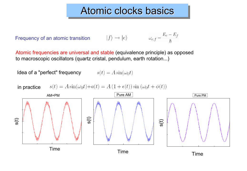
Atomic clocks basicsAtomic clocks basicsAtomic clocks basics

Frequency of an atomic transition

Atomic frequencies are universal and stable (equivalence principle) as opposedto macroscopic oscillators (quartz cristal, pendulum, earth rotation...)

Idea of a "perfect" frequency

in practices(

t)

Time

Pure AM

s(t)

Time

Pure PMAM+PM

s(t)

Time

Signal analysisSignal analysisSignal analysis

Instantaneous frequency

Frequency stability: "magnitude" of relative frequency fluctuations

Frequency Stability is characterized with the Allan variance

typical frequency fluctuations averaged over

with ,

Experimentally

converges for most of the types of noise met experimentally

- 3

0

3

White frequency noiseWhite frequency noiseWhite frequency noise

- 3

0

3

- 3

0

3

- 3

0

3

- 2

0

2

Flicker frequency noiseFlicker frequency noiseFlicker frequency noise

- 2

0

2

- 2

0

2

- 2

0

2

Frequency accuracyFrequency accuracyFrequency accuracy

The signal average frequency differs from the atomic frequency

is the sum of all possible frequency shifts (Zeeman, Stark, Collisions, Doppler...) which are evaluated from frequency measurements

Noise of the measurements (stability) ultimately determines the accuracye.g. 10-15 is reached after 104 seconds (3 hours)

10-16 after 106 seconds (10 days)

Accuracy: uncertainty on

Conversely, a good control ofthe frequency shifts is necessary toavoid long term degradation of thefrequency stability (flicker floor, frequency drift)

Accuracy and stability are strongly linked

An accuracy evaluation below 10-16 is impossible

Tjoelker et al. 1996

Atomic clock principleAtomic clock principleAtomic clock principle

0

1

atomic resonancemacroscopic oscillator

atoms

interrogation

correction

-low natural width (Cs: 10-13 Hz, Hg+: 2 Hz)-Fourier limit, long interaction time (Cs: 1 Hz, Hg+: 6 Hz)-low oscillator spectral width (Cs: 10-5 Hz, Hg+: 0.1 Hz)

-Large atom number (Cs: 107, Hg+: 1) -low noise detection scheme-low noise oscillator

-as high as possible (Cs: 10 GHz, Hg+: 1 PHz)

Cs fountain (SYRTE): 10-14 τ -1/2, accuracy 7 10-16

Optical Hg+ (NIST): 4 10-15 τ -1/2, accuracy 10-14

+ transition should be insensitive to external perturbations

atomic quality factor

Atomic FountainsAtomic FountainsAtomic Fountains

BNM-SYRTE (F) PTB (D) NIST (USA)

10 fountains in operation (SYRTE, PTB, NIST, USNO, PENN state, ON, IEN, NPL) with an accuracy of ~10-15. Several projects (NIJM, NIM, KRIISS, VNIIFTRI...)

See e.g. Proc. 6th Symp. Freq. Standards and Metrology (World Scientific 2002)

Energy levels CsEnergy levels CsEnergy levels Cs133Cs

133Cs hyperfine splitting is the basis for the definition of the SI second.

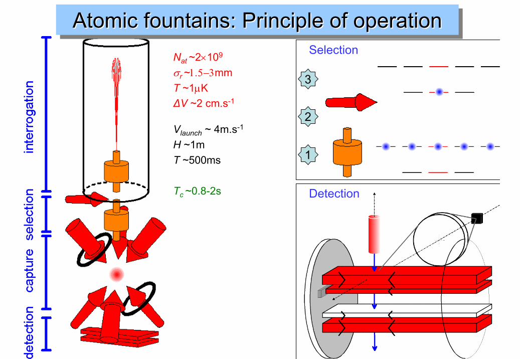
Detection

Nat ~2×109

σr ~1.5−3mmT ~1µK∆V ~2 cm.s-1

Vlaunch ~ 4m.s-1

H ~1mT ~500ms

Tc ~0.8-2s

Selection

3

2

1

Atomic fountains: Principle of operationAtomic fountains: Principle of operationAtomic fountains: Principle of operation

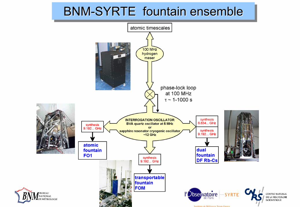
BNM-SYRTE fountain ensembleBNMBNM--SYRTE fountain ensembleSYRTE fountain ensemble

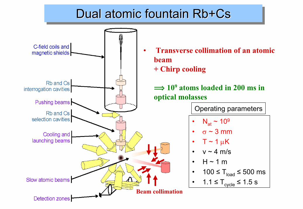
Beam collimation

• Nat ~ 109

• σ ~ 3 mm• T ~ 1 µK• v ~ 4 m/s• H ~ 1 m• 100 ≤ Tload ≤ 500 ms• 1.1 ≤ Tcycle ≤ 1.5 s

Operating parameters

Dual atomic fountain Rb+CsDual atomic fountain Dual atomic fountain Rb+CsRb+Cs

• Transverse collimation of an atomic beam+ Chirp cooling

î 109 atoms loaded in 200 ms in optical molasses

Due to the first order Doppler effect, the frequency of the upper and lower laser beam is the same in the frame moving upwards at

A key technique: The moving molassesA key technique: The moving molassesA key technique: The moving molasses

For Cs:

The area Ae and Af of the time of flight signals in calculated. The transition probability is given by

Response of the detection: area per atom

time spent in laser beam (s)

gain amp. (V.A-1)

photodiode response (A.W-1)

collection efficiency

radiated power (W)

Measurement of the transition probabilityMeasurement of the transition probabilityMeasurement of the transition probability

Technical noise ~ 400 atoms

Interrogation region with magnetic and thermal shields

Compensation coils

Optical molasses

Collimator for molasses beams

The 2 outermost shields are removed

vacuum chamber and cavityvacuum chamber and cavityvacuum chamber and cavity

optical benchoptical benchoptical benchLaser diode based system, can be made compact and reliable

Optical fibers

External cavity diode laser

Injection locked diode laser

Cs vapor cell

Acousto-optic modulator

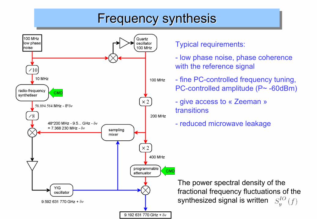
Frequency synthesisFrequency synthesisFrequency synthesis

Typical requirements:

- low phase noise, phase coherence with the reference signal

- fine PC-controlled frequency tuning, PC-controlled amplitude (P~ -60dBm)

- give access to « Zeeman » transitions

- reduced microwave leakage

The power spectral density of the fractional frequency fluctuations of the synthesized signal is written

lineshape calculationlineshapelineshape calculationcalculationInitial hypothesis: - external motion is described by a classical trajectory r(t)

- the two clock levels are spectrally resolved => 2 level atom- any process causing relaxation is neglected

Hamiltonian:

(magnetic dipole interaction, gI, ge-2 neglected)(purely stationary field)

We neglect non-resonant terms (rotating wave approximation)

We then rewrite the Hamiltonian in a new representation

Atomic observables are also transformed to the same representation

Atomic evolution using the Bloch vectorAtomic evolution using the Bloch vectorAtomic evolution using the Bloch vectorHamiltonian in the new representation

The Hamiltonian can be written as

We define the Bloch vector (or fictitious spin) as

detuning

Equation of evolution for the Bloch vector

Atomic observables

Pauli matrices

We used Heisenberg’s equations for sigma

and

Rabi oscillationsRabi oscillationsRabi oscillations

Example: Rabi oscillation on resonance (δ=0)

The Bloch vector evolves according to

The motion is an instantaneous rotation around

π/2 pulses:

Final state

3π/2 pulses:

Ramsey interrogationRamsey interrogationRamsey interrogation

The final state depends mostly on the accumulated phase during the free flight between the microwave field (ω) and oscillating atomic coherence (ωef):

1st interaction free flight

As long as δ<<Ω0:

Time

One big advantage: most of the time, atoms evolve without being coupled to the exciting field

2nd interaction

Ramsey fringes

-100 -50 0 50 1000.0

0.2

0.4

0.6

0.8

1.0

-1.0 -0.5 0.0 0.5 1.00.0

0.2

0.4

0.6

0.8

1.0

detuning (Hz)

0.94 Hz

trans

ition

pro

babi

lity

P

NO AVERAGING

ONE POINT = ONE MEASUREMENT OF P

Ramsey fringes in atomic fountainRamsey fringes in atomic fountainRamsey fringes in atomic fountain

Fluctuations of the transition probability:

We alternate measurements on bothe sides of the central fringe to generate an error signal, whichis used to servo-control the microwave source

Sensitivity functionSensitivity functionSensitivity functionGoal: to calculate the effect of temporal frequency fluctuations of the interrogation oscillator (to first order)

The sensitivity function can be used (with care) to calculate the effect of a perturbation of the atomic frequency

Definition of the sensitivity function

Important remark: In true life, the sensitivity function is not exactly the same for all atomic trajectories. In some cases, this must be accounted for.

It can be computed (and measured) by looking at the effect of a phase step during the interaction

The sensitivity function depends on the interaction scheme. It gives simple way to estimatefrequency shifts or the effect of the noise of the interrogation even for complex cases (timedependent frequency shifts, non-square pulses...).

Shape of the sensitivity functionShape of the sensitivity functionShape of the sensitivity functionFor a single centered trajectory and in the limit δ<<Ω0, this is possible to derive an analytical expression. For an optimized Ramsey interrogation, we have:

Sensitivity function in atomic fountains for two different field amplitudes Ω0

In a fountain : TE011 mode

The sensitivity function and frequency shiftsThe sensitivity function and frequency shiftsThe sensitivity function and frequency shiftsThe equilibrium condition of the loop

is developed to first order using g(t)

The fractional frequency shift is then given by

Slightly modified if we account foractual individual atomic trajectories

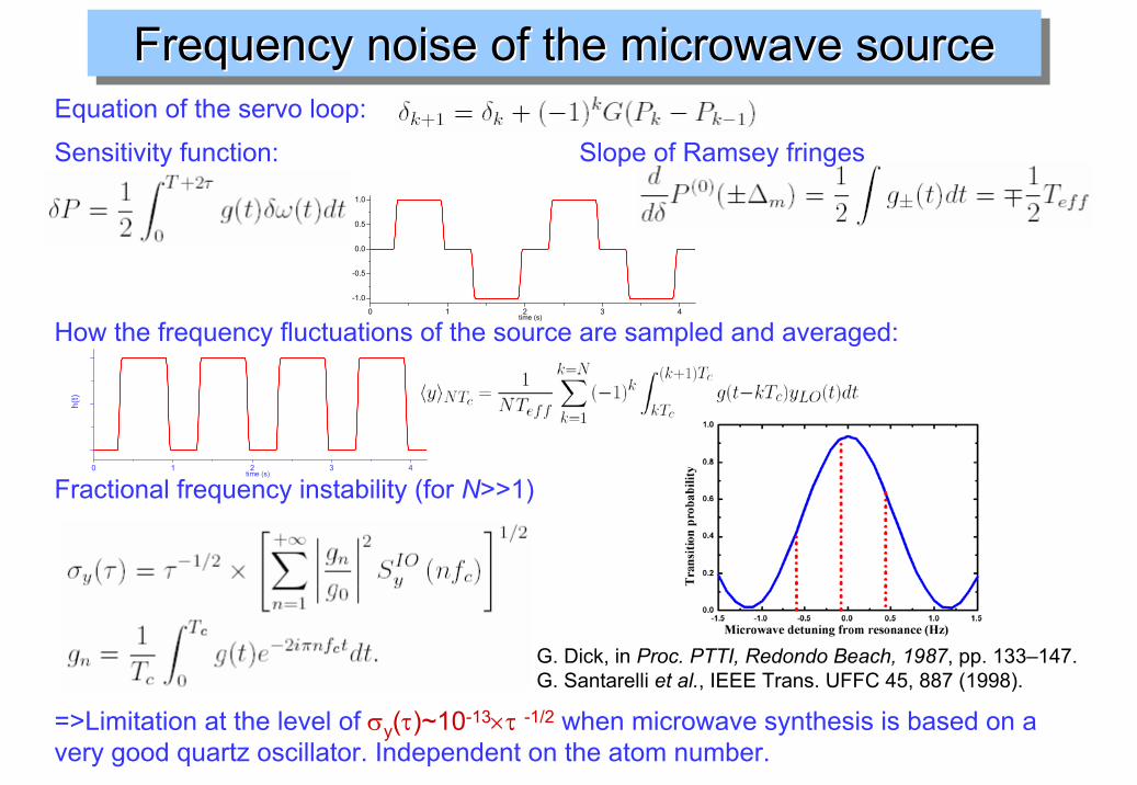
Frequency noise of the microwave sourceFrequency noise of the microwave sourceFrequency noise of the microwave sourceEquation of the servo loop:

How the frequency fluctuations of the source are sampled and averaged:

Fractional frequency instability (for N>>1)

=>Limitation at the level of σy(τ)~10-13×τ -1/2 when microwave synthesis is based on a very good quartz oscillator. Independent on the atom number.

Sensitivity function: Slope of Ramsey fringes

G. Dick, in Proc. PTTI, Redondo Beach, 1987, pp. 133–147. G. Santarelli et al., IEEE Trans. UFFC 45, 887 (1998).

Typically, when using a very good quartz oscillator:

Frequency stability: Fountain vs H-maserFrequency stability: Fountain Frequency stability: Fountain vsvs HH--masermaser

maser autotuning

integration time τ(s)

fract

iona

l fre

quen

cy in

stab

ility

Limiting term: phase noise of the quartz oscillator

Rb fountain vs. H-maser

Frequency stability: Fountain vs FountainFrequency stability: Fountain Frequency stability: Fountain vsvs FountainFountain« Loose synchronization » (within a few seconds to a few minutes)

Cycle by cycle synchronization with matched sensitivity functions: cancellation of the high frequency noise of the interrogation oscillator

Cryogenic oscillatorCryogenic oscillatorCryogenic oscillator

Sapphire cryogenic oscillator from the University of Western Australia

High quality factor sapphire resonator (Q ~ 4×109) at 12 GHzTurning point of temperature sensibility: dν/dT = 0 near T=6K

SCO has extremely good short term stability (measured at UWA against a second SCO)

SCO signal is converted to 9.2 GHz

A. Luiten, M. Tobar et al.

For a single atom: - transition probability P:

- Variance of quantum fluctuations of P:

Quantum projection noiseQuantum projection noiseQuantum projection noise

Contribution of the photon shot noise (an other quantum noise):

For an ensemble of Ndet uncorrelated atoms:

Contribution of the quantum projection noise to the frequency instability:

nph : number of detected photons per atom

Practically, nph ~ 100 and this contribution is a small (negligible) fraction of the quantum projection noise

Itano et al. PRA 47, 3554 (1993)Spin squeezing: Itano, Polzik, Mölmer…

104 105 106

10-3

10-2

0.91 Nat-1/2

σ y(τ) Q

atπ(

τ/T c)1/

2

Nat

Quantum LimitedOperation of a Cs Fountain up to Nat∼ 6 105

For Nat∼ 6 105 atoms, the frequency stability isσy(τ) ~ 4 10-14 τ-1/2

G.Santarelli et al. PRL,82,4619 (1999)

Quantum projection noiseQuantum projection noiseQuantum projection noise

FO2 frequency stability

This stability is close to the quantum limit. A resolution of 10-16 is obtained after 6 hours of integration. With Cs the frequency shift is then close to 10-13!

With a cryogenic sapphire oscillator, low noise microwave synthesis

(~ 3×10-15 @ 1s)

Frequency stability with a cryogenic Oscillator Frequency stability with a cryogenic Oscillator Frequency stability with a cryogenic Oscillator

100 1000 10000

1E-16

1E-15

1E-14

2.83 10-14

4.13 10-14

stab

ilité

de

fréqu

ence

temps (s)

FO1 FO2 Difference

5.01 10-14

Frequency comparisons between fountainsFrequency comparisons between fountainsFrequency comparisons between fountains

Fountain AccuracyFountainFountain AccuracyAccuracyFO1FO2(Rb)FO2(Cs)Fountain (BNM-SYRTE)

0.0(3.0)0.0(3.0)0.0(3.0)Residual Doppler effect

-3.3(3.3)0.0(2.0)-4.3(3.3)Microwave leaks, spectral purity, synchronous perturbations.

0.0(1.0)0.0(1.0)0.0(1.0)Collisions with residual gaz.

0.0(1.4)0.0(1.4)0.0(1.4)Recoil0.0(1.0)0.0(1.0)0.0(1.0)Neighbouring transitions.

7.5

-197.9(2.4)

-162.8(2.5)1199.7(4.5)

7

0.0(1.0)

-127.0(2.1)3207.0(4.7)

-357.5(2)Collisions + cavity pulling

-168.2(2.5)Blackbody radiation1927.3(.3)second order Zeeman

6.5Total

Effect Shift and uncertainty (10-16)

Frequency difference between FO1 and FO2: 3 10-16

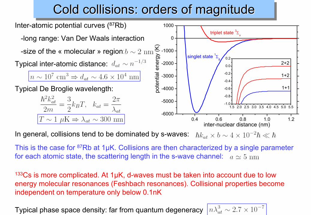
Cold collisions: orders of magnitudeCold collisions: orders of magnitudeCold collisions: orders of magnitudeInter-atomic potential curves (87Rb)

-long range: Van Der Waals interaction

-size of the « molecular » region:

Typical inter-atomic distance:

Typical phase space density: far from quantum degeneracy

Typical De Broglie wavelength:

In general, collisions tend to be dominated by s-waves:

133Cs is more complicated. At 1µK, d-waves must be taken into account due to low energy molecular resonances (Feshbach resonances). Collisional properties become independent on temperature only below 0.1nK

This is the case for 87Rb at 1µK. Collisions are then characterized by a single parameter for each atomic state, the scattering length in the s-wave channel:

0.4 0.6 0.8 1.0 1.2-6000

-5000

-4000

-3000

-2000

-1000

0

1000

1.5 2.0 2.5 3.0 3.5 4.0 4.5 5.0 5.5-1.0

-0.8

-0.6

-0.4

-0.2

0.0

0.2

pote

ntia

l ene

rgy

(K)

inter-nuclear distance (nm)

singlet state 1Σg

triplet state 3Σu

1+1

1+2

2+2

Total mean-field interaction energy as a function of scattering length aff, atomic density n, atom number Nat and atomic mass m:

Energy conservation before/after the interaction (with only the clock states populated and assuming 100% transfer efficiency)

Resulting clock shift:

In general (other states populated), the instantaneous frequency shift of the atomic resonance is given by:

In the fountain, the time variation of the atomic density must be taken into account with the sensitivity function

Mean-field energy and collisional shiftMeanMean--field energy and field energy and collisionalcollisional shiftshift

Collisional shift : 87Rb vs 133CsCollisionalCollisional shift : 87Rb shift : 87Rb vsvs 133Cs133Cs

SYRTE

YALE

Th.

The shift in 87Rb is much (~50 to 100 times) smaller than in 133Cs

Atomic density changed by changing the trapping light intensity (40% uncertainty)

Differential measurements (interrogation oscillator H-maser)

In a MOT

Cavity pulling is taken into account and subtracted

SYRTE Y. Sortais et al. , PRL, 85, 3117 (2000)Th.1 = -11.7×10-23/ (at.cm-3) (S. Kokkelmans et. al., PRA 56, R4389 (1997))Th.2 = -7.2×10-23/ (at.cm-3) (C.Williams et al.)YALE -5.6 ( ± 3.3)×10-23/ (at.cm-3); (C.Fertig and K.Gibble, PRL, 85, 1622 (2000))

Collisional shift measurementCollisionalCollisional shift measurementshift measurement

By performing the internal state selection with adiabatic passage, we vary the atomic density by a factor of 2 without changing velocity and position distribution

Cold collisions then only depend on the atomic number

To measure the cold collision shift in quasi real time

We alternate measurements with full or interrupted adiabatic passage (produces n or n/2)

Launching

Sweeping

Pushing

F. Pereira Dos Santos et al., PRL 89,233004 (2002)

|->

|+> |3,n>

|4,n-1>

|4,n-1>

|3,n>

δ

0 1 2 3 4

-5

0

5

Det

unin

g (k

Hz)

Time (ms)0 1 2 3 4

0

2

4

6

Rab

i Fre

quen

cy (k

Hz)

Time (ms)100% 50%

The “adiabatic passage method”: ExperimentsThe “adiabatic passage method”: ExperimentsThe “adiabatic passage method”: Experiments

We have a practical realization of two atomic samples with a density ratio precisely equal to 1/2

Extrapolation of the collisionalshift:

MEASURED

The value and the stability of the ratio between 50% and 100% configurations is monitored during each measurement. We find:

Adiabatic passage method limitationAdiabatic passage method limitationAdiabatic passage method limitationOne of the possible limitation of the adiabatic passage method: off-resonant optical pumping due to the pushing beam

Measured atom number ratios with adiabatic passage

The effect of spurious mF states is studied by populating them purposely and selectively

With adiabatic passage and differential measurement, the measured quantity is the ratio between contributions of mF=0 states and the other mF state

⇒the atomic density cancels out

⇒possibility of precise comparison with theory

Ratio between the shift per atom due to the 0 states (ν00) and to the mF state (νmFmF)

The contribution of m F ≠ 0 states are at most 1/3 of the contribution of the clock states

In the usual clock configuration: 3×10-3 residual populations in mFstates contributes to less than 1×10-3

The cold collisional shift can be controlled at 10-3 of its value

Effect of the mF≠0 statesEffect of the mEffect of the mFF≠≠0 states0 statesDifferential method with 3 different configurations (period 60 cycles):

1. Full density on (0-0) 2. half density on (0-0)

3. Full density on (0-0) and on (mF - mF), (additional synthesizer for m F ≠ 0)

Clock shifts due to |mF| = 3 are not equal …

Feshbach resonances at low magnetic field (Cs)Feshbach resonances at low magnetic field (Cs)Feshbach resonances at low magnetic field (Cs)

Ratio of frequency shift due to |mF| = 1; 2; 3 over clock states frequency shift plotted as functions of the magnetic field.

Observation of the amplitude (all mF) and the width (|mF| = 3) of Feshbach resonances.

Calibration of the relative contribution of the remaining mF ≠ 0 atoms on the clock shift with respect to the B fieldH. Marion et al. to be published

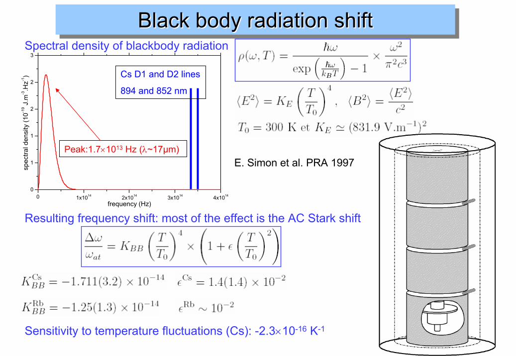
Black body radiation shiftBlack body radiation shiftBlack body radiation shiftSpectral density of blackbody radiation

Cs D1 and D2 lines

894 and 852 nm

Peak:1.7×1013 Hz (λ~17µm)

Resulting frequency shift: most of the effect is the AC Stark shift

Sensitivity to temperature fluctuations (Cs): -2.3×10-16 K-1

E. Simon et al. PRA 1997

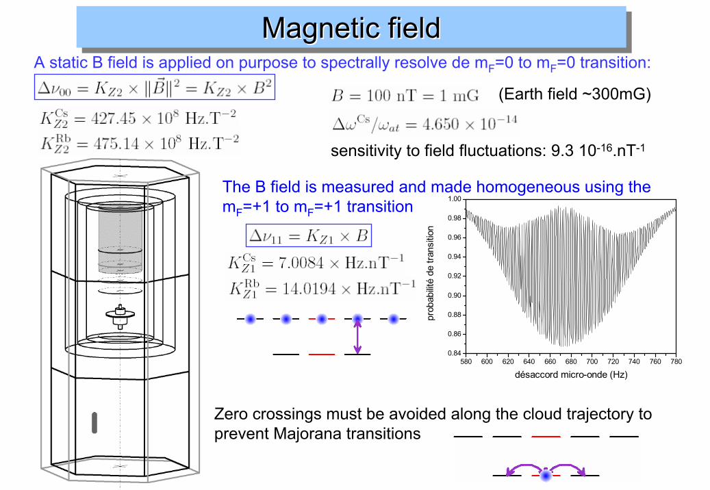
Magnetic fieldMagnetic fieldMagnetic fieldA static B field is applied on purpose to spectrally resolve de mF=0 to mF=0 transition:

(Earth field ~300mG)

sensitivity to field fluctuations: 9.3 10-16.nT-1

The B field is measured and made homogeneous using the mF=+1 to mF=+1 transition

Zero crossings must be avoided along the cloud trajectory to prevent Majorana transitions

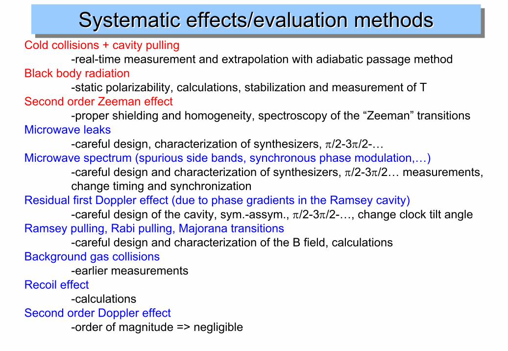
Cold collisions + cavity pulling-real-time measurement and extrapolation with adiabatic passage method

Black body radiation-static polarizability, calculations, stabilization and measurement of T

Second order Zeeman effect-proper shielding and homogeneity, spectroscopy of the “Zeeman” transitions

Microwave leaks-careful design, characterization of synthesizers, π/2-3π/2-…

Microwave spectrum (spurious side bands, synchronous phase modulation,…)-careful design and characterization of synthesizers, π/2-3π/2… measurements, change timing and synchronization

Residual first Doppler effect (due to phase gradients in the Ramsey cavity)-careful design of the cavity, sym.-assym., π/2-3π/2-…, change clock tilt angle

Ramsey pulling, Rabi pulling, Majorana transitions-careful design and characterization of the B field, calculations

Background gas collisions-earlier measurements

Recoil effect-calculations

Second order Doppler effect-order of magnitude => negligible

Systematic effects/evaluation methodsSystematic effects/evaluation methodsSystematic effects/evaluation methods

PHARAO: a Transportable FountainPHARAO: a Transportable PHARAO: a Transportable FountainFountain

vacuum chamber

atomic hydrogenFaraday cage

time resolvedphoton counting

2S detector

cryostat

chopper

dye laser486 nm

microwaveinteraction

cold atomsource

detection70 fs Ti:sapphiremode locked laser

1/2 x f dye

λ

I

9.2 GHz

4/7 x f dye

f dye

243 nm

x1/2x4/7

x 2 ν1S-2S = 2 466 061 413 187 103 (46) HzAccuracy : 1.8 10-14

Measurement of 1S-2S transition of Hydrogen at Max Planck Institut fürQuantenoptik in Garching

M. Niering et al, PRL 845, 5496 (2000)

Measurement of the Ry, test of QED,fundamental constants stability.

Frequency Comparison NIST F1 - CSF1

(period of overlap, date of measurement)

Number of Measurement0 1 2 3 4

1015

x y(F

1 - C

SF1)

-6

-4

-2

0

2

4

(15 days, August 2000)

(10 days, July 2001) (20 days, November 2001)

Long distance comparison between PTB and NIST Cesium Fountains

Long distance Long distance comparisoncomparison betweenbetween PTB PTB andand NIST NIST CesiumCesium FountainsFountains

BIPM circular Tdata base ofclock comparisonsusing GPS or TWSTFT

PTB: A. Bauch, S. WeyersNIST: S. Jefferts

Microwave frequencies• Cs 9.192 631 770 GHz• 87Rb 6.834 682 610… GHz

Magneto-optical trap or molasses.

108 atomes, T ~1µK

Resonance width ~1Hz

Frequency stability: 1 10-14 τ -1/2

Frequency accuracy : 7 10 -16

Atomic fountains: summaryAtomicAtomic fountainsfountains: : summarysummary

Ultimate accuracy~10-16

Can we go further ?

Two possible waysTwo possible waysTwo possible ways

0

1

atomic resonancemacroscopic oscillator

atoms

interrogation

correction

-low natural width-Fourier limit, long interaction time-low oscillator spectral width

-Large atom number-low noise detection scheme-low noise oscillator

-as high as possible + transition should be insensitive to external perturbations

atomic quality factor

Atomic transition in the optical domain

A clock in space

Optical frequency standards ?Optical frequency standards ?Optical frequency standards ?

Frequency stability :

Increase (x 105)

Frequency accuracy: most of the shifts (expressed in absolute values) don't dependon the frequency of the transition (Collisions, Zeeman...).

Three major difficulties

-Ability to compare frequencies (no fast enough electronics )

-Recoil and first order Doppler effect

-Interrogation oscillator noise conversion (Dick effect).

Optical fountain at the quantum limit !!!!!!!!!

The best optical clocks so far exhibit frequency stabilities in the 10-15 τ -1/2 range togetherwith an accuracy around 10-14.

Optical frequency measurementsOptical frequency measurementsOptical frequency measurements

Harmonic frequency chains: -A set (about 13) of non linear stages, each of them performing a basic operation(frequency multiplication by 2 or3, addition, difference).-Uncomfortable regions of the spectrum (THz, MIR): alcohol lasers…-1 apparatus for one particular transition (to within a few 10's GHz).-very heavy and complex systems (need for secondary standards).

No electronics is fast enough to measure the phase of signals @ frequencies > ~100 GHz

Only a few systems have been fully operated (JILA, PTB, SYRTE, NRC).

divide by 3 system

Schnatz H. et al. PRL 76 18 (1996)Only one achieved phase coherent comparison visible-RF

• temporal domain

• frequency domain

0

I(f)

f

2∆φ

τr.t = 1/fr

t

E(t) ∆φ

Femto-second frequency chainFemtoFemto--second frequency chainsecond frequency chain

x2

x

All optical frequencies of the comb are known in terms of RF frequencies

J. Reichert et al. PRL 84, 3232 (2000), S. Diddams et al. PRL 84,5102 (2000)

Femtosecond Laser FemtosecondFemtosecond Laser Laser

Kerr effect mode lockedTi-Sa laser (25fs)450 mW outputSpectral broadeningusing a photonic crystalfiber (up to 270 mwoutput)Self referencedfrequency comb

40µm

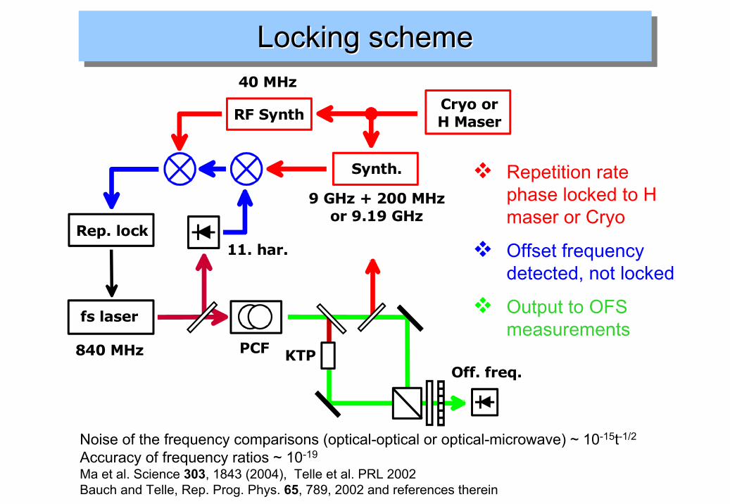
Locking schemeLockingLocking schemescheme

Repetition rate phase locked to H maser or Cryo

Offset frequencydetected, not locked

Output to OFS measurements

Synth.

RF Synth

Rep. lock

fs laser

PCF

Off. freq.

Cryo orH Maser

KTP840 MHz

9 GHz + 200 MHzor 9.19 GHz

40 MHz

11. har.

Noise of the frequency comparisons (optical-optical or optical-microwave) ~ 10-15t-1/2

Accuracy of frequency ratios ~ 10-19

Ma et al. Science 303, 1843 (2004), Telle et al. PRL 2002Bauch and Telle, Rep. Prog. Phys. 65, 789, 2002 and references therein

Recoil effectRecoil effectRecoil effect

Overlap of the wave packets after 1s offree flight would imply temperatures ~ 1 fK

Ramsey-Bordé interferometer

Experimental realisation: PTB, NIST (Ca atoms) G. Wilpers et al., PRL 89 230801 (2002)C. W. Oates et al. Opt. Lett. 25, 1603 (2000).

C. Bordé et al. PRA 30 1836 (1984)

Ca optical clockCa optical clockCa optical clock

Ca Vs Maser

Ca Vs cavity

Ca Vs Hg+

First order Doppler effect (wavefront curvature,beam misalignement).

Dick effect (very low duty cycle)

Trapped particles (Lamb-Dicke regime)Trapped particles (LambTrapped particles (Lamb--DickeDicke regime)regime)

classical picture

To first order, no effect of the atomic motion

quantum pictureMomentum conservation

if the atom is confined to well below λ, is a broad function of p

The atomic transition is not shifted or broadened (Recoil, Doppler)

Very detailed calculations in Wineland, Itano PRA 20, 1521 (1979)

For atoms, however, conservative traps require large trapping fields inducing large shifts of the levelsions can be trapped with much lower fields, but with only a few ions in the trap for a clock

Single ion clockSingle ion clockSingle ion clock

Other experiments: NPL : Yb+, Sr+, NRC : Sr+, MPQ : In+…

Yb+, PTB (Tamm, Peik...)Hg+, NIST (Bergquist et al.)

R. Rafac, B. Young, J. Beall, W. Itano, D. Wineland and J. Bergquist, PRL 85, 2462 (2000)

Width

40 Hz

10 Hz

20 Hz

6 Hz

Quality factor: Q = ν/∆ν=1.6 1014

Highest Q ever achievedCurrent accuracy: 10-14

NIST Hg+ ClockNIST Hg+ ClockNIST Hg+ Clock

NIST Hg+ Clock accuracyNIST HgNIST Hg++ Clock accuracyClock accuracy

Effect Correction UncertaintySecond order Zeeman effect @ B=2.7 G

+1 386 2.6

Black Body radiation shift @ T=300K

+0.079 <0.08

Black Body radiation shift @ T=4K

0 0

Second order Doppler secular motion

<0.003 0.003

Second order Doppler micromotion

<0.1 0.1

Background collisions (4He) 0 <1 Quadrupole shift @ ∇E=10 V.mm-2

0 10

Quadratic sum 10 Hz

At PTB sub Hz comparison of Yb+ single ion clocks (Tamm et al. Proc. ICOLS 2003, arXiv 0403120)

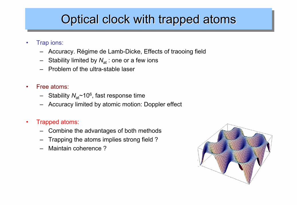
Optical clock with trapped atomsOpticalOptical clockclock withwith trappedtrapped atomsatoms

• Trap ions: – Accuracy. Régime de Lamb-Dicke, Effects of traooing field– Stability limited by Nat : one or a few ions– Problem of the ultra-stable laser

• Free atoms:– Stability Nat~106, fast response time– Accuracy limited by atomic motion: Doppler effect

• Trapped atoms:– Combine the advantages of both methods– Trapping the atoms implies strong field ?– Maintain coherence ?

A future optical standard withtrapped Atoms

A future A future opticaloptical standard standard withwithtrappedtrapped AtomsAtoms

3P01

461 nm

689 nm

698 nm(87Sr: 1 mHz)

1S0

1P1

3S1688 nm

679 nm

λtrap

λtrap

Katori, Proc. 6th Symp. Freq. Standards and Metrology (2002)Pal’chikov, Domnin and Novoselov J. Opt. B. 5 (2003) S131Katori et al. PRL 91, 173005 (2003)

Clock transition 1S0-3P0 transition (Γ =1mHz)

Combine advantages of single trapped ion andFree fall neutral atoms optical standards

Sr 1S0-3P0 transitionSrSr 11SS00--33PP00 transitiontransition

ν1S0-3P0=429 228 004 235 (20) kHz

-4 -3 -2 -1 0 1 2 3 499.0

99.2

99.4

99.6

99.8

100.0

MO

T flu

ores

cenc

e (%

)

698 nm laser detuning from resonance (MHz)

Courtillot et al., PRA 68, 030501 (2003).

Free Falling atoms

Trapped atomsTakamoto et al. PRL 91, 223001 (2003)

Magic wavelength measurement (813 nm)Very recently linewidth 50 Hz (Katori ICAP 2004)

Other experiements (JILA, PTB, LENS, NIST…)Other atoms: Yb, Hg…

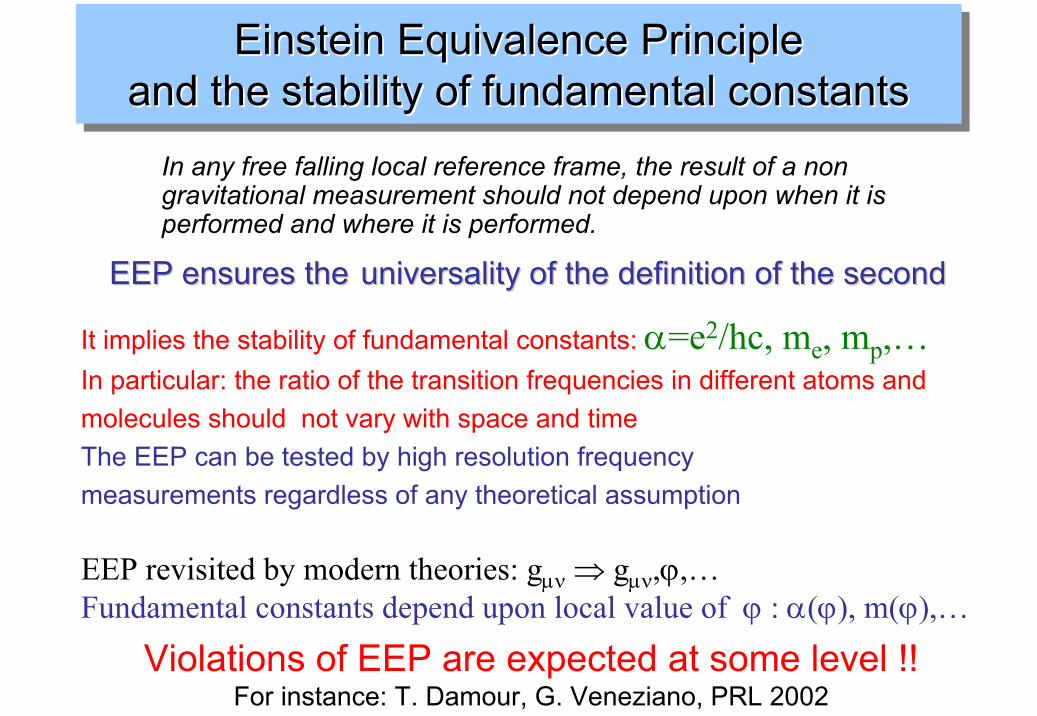
Einstein Equivalence Principleand the stability of fundamental constants

Einstein Equivalence Einstein Equivalence PrinciplePrincipleandand thethe stabilitystability ofof fundamentalfundamental constantsconstants

It implies the stability of fundamental constants: α=e2/hc, me, mp,…In particular: the ratio of the transition frequencies in different atoms andmolecules should not vary with space and timeThe EEP can be tested by high resolution frequencymeasurements regardless of any theoretical assumption

EEP revisited by modern theories: gµν ⇒ gµν,ϕ,…Fundamental constants depend upon local value of ϕ : α(ϕ), m(ϕ),…

EEP EEP ensuresensures thethe universalityuniversality of of thethe definitiondefinition of of thethe secondsecond

Violations of EEP are expected at some level !!For instance: T. Damour, G. Veneziano, PRL 2002

In any free falling local reference frame, the result of a non gravitational measurement should not depend upon when it isperformed and where it is performed.

Does the fine structure constant α varies ? DoesDoes thethe fine structure constant fine structure constant αα varies ? varies ?

Because of large relativistic corrections, the hyperfine energy of an alkali atomdepends upon Z and α=e2/ħc

Search method for α drift:

Compare hyperfine energy of rubidium and cesium as function of time

– Oklo test : geochemical analysis of the natural fossil fission reactor in Oklo (Gabon, 1.8×109 yr ago) :

Damour, Poliakov, Nucl. Phys. B 480, 37 (1996)– Absorption spectroscopy from quasars:

J. Webb et al., PRL 87, 091301 (2001)

( ) )5.35.0(1018.072.0 5 <<×±−=∆ − zαα

7101 −×≤− Oklonow αα 117105 −−×≤ yrαα&

Present tests of cosmologicalVariations of α

PresentPresent tests tests ofof cosmologicalcosmologicalVariations Variations ofof αα

• A priori loss of factor 1010 in sensitivity !!• ~ 1 year versus 1010 years• But: • ultra-stable and accurate clocks:• 10-15 10-16 -10-17

• repeatable measurements• independent checks in various labs• choice of hyperfine, fine and optical transitions

Laboratory tests versus cosmological testsLaboratoryLaboratory tests versus tests versus cosmologicalcosmological teststests

See S. Karshenboim, Can. J. Phys 78 639, (2000), J.P. Uzan Rev. Mod. Phys., 75, 403 (2002)

Test of Local Position InvarianceStability of fundamental constants (1)

Test of Local Position InvarianceTest of Local Position InvarianceStability of fundamental constants (1)Stability of fundamental constants (1)

Frequency of hyperfine transitions as a function of fundamental constants (at lowest order):

atomic unit of frequency nuclear g-factor

electron to proton mass ratiopurely numerical factor

relativistic « correction » factor, function of the fine structure constant α

Frequency of electronic transitions as a function of fundamental constants (at lowest order):

Ratio between atomic frequencies:

Sensitivity to variation of fundamental constants:

[Following the work of Prestage et al., PRL 74, 3511 (1995)]



g(i) and mp are not “fundamental” constants but they can be linked (at least in principle) to 2 fundamental parameters:

Any clock comparison can be seen as testing the stability of 3 fundamental parameters:

The K(i) are sensitivity coefficients:

With 4 well chosen atomic clocks, we constrain the stability of 3 independent frequency ratios => independent constraint to the variation of

mass scale of QCD: quark mass:

[Following the work of V.V. Flambaum, ArXiv:physics/0302015 (2003)]

hfs:

elec:

molecular vibration:

With more than 4 well chosen atomic clocks, redundancy is achieved



Comparisons between 87Rb and 133Cs hyperfine frequencies in atomic fountains over 5 years: one data point on this graph corresponds to

~2 months of measurements, with many checks on systematic shifts

early measurement with a fractional uncertainty 1.3×10-14. Improvement by 104 at the time.

latest measurements with a fractional uncertainty 1.3×10-15:

Stability of fundamental constants:

Other recent comparison 199Hg+(elec) vs. 133Cs(hfs) at NIST:

Marion et al. PRL 90, 150801 (2003)

Bize et al. PRL 90, 150802 (2003)



Other Measurements with comparable accuracy (H, Yb+)

Bize et al. PRL 90, 150802 (2003)Fischer et al. arXiv:physics 0311128 and 0312086, PRL 2004 Peik et al., arXiv:physics 0402132 (2004)

A FEW REFERENCESA FEW REFERENCESA FEW REFERENCES

Vannier, Audoin, "the quantum physics of atomic frequency standards" Adam Hilger (1989)

A. Bauch, H. Telle,"frequency standards and frequency measurements" Rep. Prog. Phys. 65, 789, (2002)

S. Cundiff and J. Ye "femtosecond optical frequency combs", Rev. Mod. Phys. 75, 325 (2003)

Proc. 6th Symp. Freq. Standards and Metrology, World scientific, (2002)

www.bipm.fr

www.nist.gov

www.ptb.de

www.obspm.fr

….

atomic clocks with cold atoms - phlam

Documents