AECL-6829

ATOMIC ENERGY £ F ^ ^ L'ENERGIE ATOMIQUEOF CANADA LIMITED ^ « S j 7 DU CANADA, LIMITEE

A COMPUTER-AIDED SURFACE ROUGHNESS MEASUREMENT SYSTEM

SYSTEME DE MESURE DE LA RUGOSiTE

DE SURFACES ASSISTE PAR ORDINATEUR

F. J. Hughes, M. H. Schankula

Whiteshell Nuclear Research Etablissement derecherchesEstablishment nucleaires de Whiteshell

Pinawa, Manitoba ROE 1 LONovember 1983 novembre

\

Copyright C Atomic Energy of Canada Limited, 1983

\

ATOMIC ENERGY OF CANADA LIMITED

A COMPUTER-AIDED SURFACE ROUGHNESS

MEASUREMENT SYSTEM

by

F.J. Hughes and M.H. Schankula

Whiteshell Nuclear Research EstablishmentPinawa, Manitoba ROE 1L0

1983 NovemberAECL-6829

\

SYSTEME DE MESURE DE LA RUGOSITE

DE SURFACES ASSISTÉ PAR ORDINATEUR

par

F.J. Hughes et M.H. Schankula

RESUME

On se sert d'un profilomètre à style diamant assisté par un systè-

me d'acquisition/d'analyse de données sur ordinateur pour caractériser les

surfaces d'éléments et de matériaux de réacteurs et examiner les effets de

topographie des surfaces sur la conductance thermique de contact.

On décrit le système actuel; on examine les problèmes de mesure et

le développement du système dans l'ensemble et on décrit les améliorations

futures possibles.

L'Énergie Atomique du Canada, LimitéeÉtablissement de recherches nucléaires de Whiteshell

Pinawa, Manitoba ROE 1L01983 novembre

AECL-6829

A COMPUTER-AIDED SURFACE ROUGHNESS

MEASUREMENT SYSTEM

by

F.J. Hughes and M.H. Schankula

ABSTRACT

A diamond stylus profilometer with computer-based data acquisi-

tion/analysis system is being used to characterize surfaces of reactor

components and materials, and to examine the effects of surface topography

on thermal contact conductance.

The current system is described; measurement problems and system

development are discussed in general terms and possible future improvements

are outlined.

Atomic Energy of Canada LimitedWhiteshell Nuclear Research Establishment

Pinawa, Manitoba ROE 1L01983 November

AECL-6829

\

CONTENTS

Page

1. INTRODUCTION 1

2. SURFACE PARAMETERS AND THE STATISTICAL PROPERTIES OF SURFACES 1

2.1 SURFACE TEXTURE PARAMETERS 12.2 BEARING AREA CURVE AND HIGH SPOT COUNT 22.3 STATISTICAL PROPERTIES 2

3. THE BASIC TALYSURF 4 SURFACE MEASUREMENT SYSTEM '3

4. SYSTEM LIMITATIONS AND MODIFICATIONS 3

4.1 DATUM 34.2 NOISE 44.3 RELOCATION 4

4.4 SURFACE DAMAGE 5

5. DATA ACQUISITION SYSTEM 5

6. DATA REDUCTION 5

7. ACCURACY AND REPRODUCIBILITY 9

8. TYPICAL RESULTS 10

9. FURTHER DEVELOPMENT , 11

10. CONCLUSIONS 11

ACKNOWLEDGEMENTS 12

REFERENCES 12

TABLES 13

FIGURES 15

\

1. INTRODUCTION

The nature of surfaces and their mechanics of contact are impor-tant in many areas of reactor technology, e.g. the performance of staticseals, friction and wear in fuelling machine components and a variety ofapplications involving thermal contacts. In particular, the demands ofnuclear fuel development and reactor safety analyses have prompted aninterest in thermal contact conductance at interfaces between variousreactor components, such as fuel-to-sheath and pressure tube-to-calandriatube. For safety analysis we need to model the resistance to heat flowacross these various interfaces.

The resistance or conductance of an interface between two solidsurfaces depends on the number of individual contacts and on their size dis-tribution, i.e. the surface microgeometry. If a fluid is present, addi-tional heat transfer may occur by conduction across the interfacial gap, theeffective thickness of which is a function of the surface microgeometry.Real surfaces also exhibit waviness, and the microcontacts tend to clusterin groups; this can affect the rate at which contact conductance changeswith load.

The measurement and characterization of surface features istherefore indispensable in the study of surface contact phenomena, providinga valuable analysis of the size and distribution of asperities and the in-terstices between them. There are many methods for measuring the micro- ormacrogeometrical features of surfaces, including optical methods and mechan-ical methods such as oblique sectioning and profilometry. Optical methodsmay be well suited to production and quality control, but are very tediousand time-consuming for quantitative scientific work, for which methods thatdirectly measure the surface profile are preferred. The best known profi-lometry method uses a fine diamond stylus, the vertical movements of whichare amplified and recorded electrically during a surface traverse.

This report describes a surface profilometry system developed atthe Whiteshell Nuclear Research Establishment. This system is based on theTalysurf 4* stylus instrument, modified to increase its capacity for scien-tific applications. Data collection and analysis have also been automated,using a Tektronix 4C51 computer with specially developed software.

2. SURFACE PARAMETERS AND THE STATISTICAL PROPERTIES OF SURFACES

2.1 SURFACE TEXTURE PARAMETERS

The most common parameters for describing surface texture are:

Centre-line-average (C.L.A.) roughness value (sometimes referredto as R ), defined as the arithmetic average of the vertical

Trade name of Rank Taylor Hobson, Leicester, England.

- 2 -

deviation of the profile from the centre line (see Figures 1and 2).

Root-mean-square (R.M.S.) roughness value, defined as the squareroot of the arithmetic mean square of the vertical deviation fromthe centre line.

The centre line is the line that divides the profile such that thesums of the enclosed areas above and below it are equal (Figure 2). Thiscentre or mean line varies in level from one profile to another and Is lo-cated at a level that is dependent on the shape and width of the surface Ir-regularities, as illustrated in Figure 3. Only in a perfectly symmetricalprofile (Figure 3D) Is the mean line coincident with the mid-height linethrough the profile. Surface texture cannot be adequately defined in termsof C.L.A. or R.M.S. roughness values, however, as these parameters can besimilar for profiles of very different types and shapes.

2.2 BEARING AREA CURVE AND HIGH SPOT COUNT

The inadequacy of single numerical parameters to define surfacetexture was recognized by Abbott and Firestone [1], who developed a methodfor deriving a bearing area (B.A.) curve for a surface profile more than45 years ago. The B.A. is the ratio of the length of material intersectingthe profile at a selected slice level through the surface, to the total mea-sured length, usually expressed as a percentage (Figure 4). The high spotcount (H.S.C.) is a measure of the number of high spots occurring in a tra-verse length at a selected slice level. The derivation of B.A. and H.S.C.curves is shown in Figure 5, which also shows how these two curves differ-entiate between profiles of different shape, but with similar C.L.A. andR.M.S. roughness values. For example, if the measured profile were in-verted, the H.S.C. curve would also be inverted and the bearing area curvewould change accordingly.

2.3 STATISTICAL PROPERTIES

A random surface profile can be defined statistically, where theprobability of finding an ordinate at a value between y and y + dy is givenby t(y)dy. The height distribution of many engineering surfaces is assumedto be Gaussian, or normal, with the density function *(y) given by

= - ~ exp(-y2/2a2) (1)

In statistical terms, the R.M.S. roughness, a, is the standard de-viation of the height distribution, and the B.A. curve can be regarded as agraph of cumulative height distribution. Other parameters of interest insurface contact phenomena are the average slope of the asperities and theaverage curvature of the peaks and valleys. Determination of these parame-ters is described later in this report.

- 3 -

3. THE BASIC TALYSURF 4 SURFACE MEASUREMENT SYSTEM

The basic Talysurf 4 profilometer system (see Figures 6 and 7)comprises a stand (A) (base, column, and V-block), gearbox (B), standardpick-up (C), electronic unit with averaging meter (D) and a rectilinearelectrograph recorder (E). The Talysurf modulated carrier instrument hasbeen described, along with other instruments and surface measurementtechniques, by R.E. Reason [2].

The pick-up has a diamond stylus tip width of 0.0025 mm that isapplied with a force of about 0.1 g. The pick-up will follow accurately thebottom of valleys >_ 0.005 mm wide, and provides a fair representation ofnarrower valleys. The traverse length is 11 mm at speeds of 3.6, 18.3 or91.4 mm'rnin . The averaging meter (for R measurements) is a non-fluctuating, integrating type with cut-off values of 0.25, 0.8 and 2.5 mm,complying with both British and American standards (BS1134:1961 andB46-1965, respectively). Vertical magnification can be as high as100 000 X. The recorder plots the amplified, demodulated, but unfilteredsignal from the pick-up (the signal to the R meter is filtered). TheH.S.C. and B.A. meter (F) provides the number of high spots in the traversedlength and the percentage bearing area. Its level control allows selectionof up to 201 different levels through the surface profile.

4. SYSTEM LIMITATIONS AND MODIFICATIONS

4.1 DATUM

Initial measurements were carried out using the basic Talysurf 4instrument with a skid nose piece on the standard pick-up. The range of Rvalues observed for zirconium alloy specimens was extremely wide and the a

values were not reproducible when multiple measurements were taken withoutdisturbing the specimen. The surface profile changes observed during suc-cessive measurements indicated that the stylus and/or skid were causingsurface deformation. Subsequent examination (see Figure 8) of selectedspecimens under a scanning electron microscope confirmed deformation by boththe skid and stylus, principally the former, depending on the amount ofcontact during set-up and the number of passes. Surface deformation by theskid was found on all zirconium alloy materials examined; it was not uniformalong the trace length and we felt that it may be compounding the erroralready introduced by using the skid nose piece itself. Since the skid isthe measurement datum and traverses the same surface as the stylus, thedatum is therefore constantly changing and consequently a small degree oferror is introduced, the extent of which is dependent on the nature of thesurface.

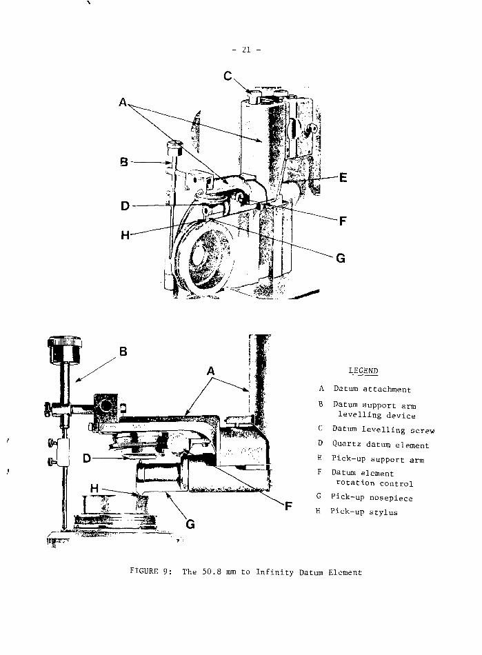
To circumvent this problem, a 50.8 mm to infinity datum element(Figure 9) was added to the Talysurf 4 to provide an independent datum, withthe stylus being the only point of contact with the surface being measured.In setting up the instrument for each measurement, the tilt and angle of thedatum can be adjusted to make it parallel to the surface. When making theadjustment, care is taken to contact the specimen only at the start, centre

- 4 -

and end of the traverse, to avoid tracking the stylus over the entiretraverse length. Using this procedure, only two traverses were required foreach measurement, one at low horizontal magnification to obtain R valuesfrom the averaging meter, and one at high horizontal magnification toprovide a recorder graph for manual analysis. The skid war therebyeliminated and surface deformation by the stylus minimized.

4.2 NOISE

Output signal noise can result from background vibration, mechani-cal noise in the pick-up and gearbox, and electrical noise in the electronicsystem.

Background vibration was measured with the stylus stationary.Figure 10(a) (100 000 X magnification) and Table 1 (line a) show the re-sults. Experience has shown that fuel sheathing and pressure tubing have Rvalues as low as 0.10 ym, of which this background vibration would represent31%.

To dampen these vibrations, an air-supported granite table mount-ing was developed. Using aircraft tire tubes in metal rings and inflatingthese with a regulated air supply, the granite block could be "floated" fromits supports (Figure 11). Repeating the vibration measurements provided thedata in Figure 10(b) and Table 1 (line b). It is seen that the R value hasdropped by a factor of 5.74, to 0.0054 jim (5.4% of that for a smooth fuel-sheath surface and an acceptable level for our work). These measurementsalso included electrical noise, but no mechanical noise.

Electrical noise was measured with a freely suspended stylus. Thedata are shown in Table 1 (line c). The electrical contribution to thetotal noise is extremely small.

A total system noise measurement enables us to determine themechanical contribution. These measurements were made by traversing thestylus across an optical flat. The R value (which includes the roughnessof the optical flat) was 0.0082 um, or 8.2% of that for a smooth fuel sheath(see Table 1 (line d)). Since the measurements were made with the tablefloating, subtraction indicates that the mechanical contribution (includingthat due to the roughness of the optical flat) is 0.0028 um. This isacceptable for our work. Further refinement of the mechanical system wouldbe extremely difficult and costly.

4.3 RELOCATION

Many surface roughness measurements are made to determine changesin a surface as the result of some secondary treatment or during the courseof an experiment. Because of variations in surface topography, we mustmeasure along the same trace as accurately as possible to determine any realchanges in characteristics. To permit this, an accurate relocation turn-table (Figure 12) was developed [3], which enables a number of reproducibleindividual traces of a surface to be made before and after secondary treat-ment, by relocation of specimens to within 0.05 |im of the original position.The surface can also be rotated to reveal directional characteristics and toprovide data for topographical maps.

\

- 5 -

4.4 SURFACE DAMAGE

Because surface texture Is so important to thermal contact conduc-tance, manual extraction of B.A. and H.S.C. curves from recorder graphs isinadequate. At best, a limited number of data points are obtained with lim-ited accuracy, by an extremely tedious and time-consuming process* Measure-ments using the H.S.C. and B.A. meter involved some 40 to 60 passes over thesame stylus trace for a through-surface analysis. Examination of zirconiumalloy specimens in a scanning electron microscope cfter such a series ofmeasurements revealed deformation by the stylus regardless of the type ofpick-up. A large error was therefore being introduced with each subsequenttraverse of the stylus. Measurements on harder U0~ fuel pellet surfacesproved to be more reproducible. The only problem experienced was bouncingof the stylus at the highest traversing speed on some of the roughersurfaces.

For our applications, we decided that the only accurate means ofmeasurement using the Talysurf 4 would be to record th& data from a singletraverse of the stylus over the surface at the lowest traversing speed.Consequently, a microcomputer-based data acquisition system was adapted toprovide single-trace analysis. This system is described in the twofollowing sections.

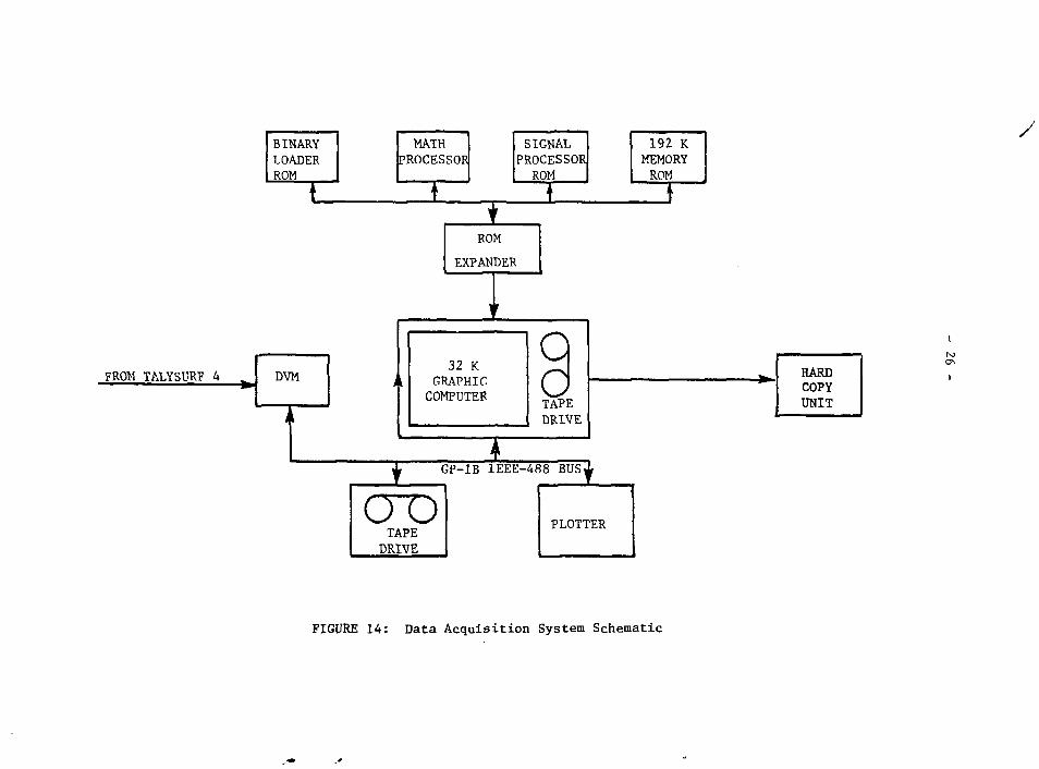
5. DATA ACQUISITION SYSTEM

The data-acquisition system (Figure 13) consists of a Tektronix4051 graphic computer (A) with built-in tape drive and storage CRT. Anexternal auxiliary tape drive (B) provides independent data transfer undermanual or program control. The electronic signals from the stylus are fedto an 8500A digital voltmeter (D.V.M.) (C) which is microprocessor-controlled. A hard-copy unit (D) and an X-Y plotter (E) provide on-linedata display.

For data acquisition (see Figure 14) the unfiltered signal inputto the Talysurf 4 recorder is also input to the D.V.M., digitized, andstored on tape at the external tape drive, from which It is transferred tothe computer. There, it is reduced to provide the required parameters, andgraphs of H.S.C. and B.A. at the plotter. At the highest horizontal magni-fication (100 X) the stylus traverse speed is 0.06 nrnvs , with a data pointtaken every 1.204 pm.

6. DATA REDUCTION

The parameters derived by the data reduction program are:

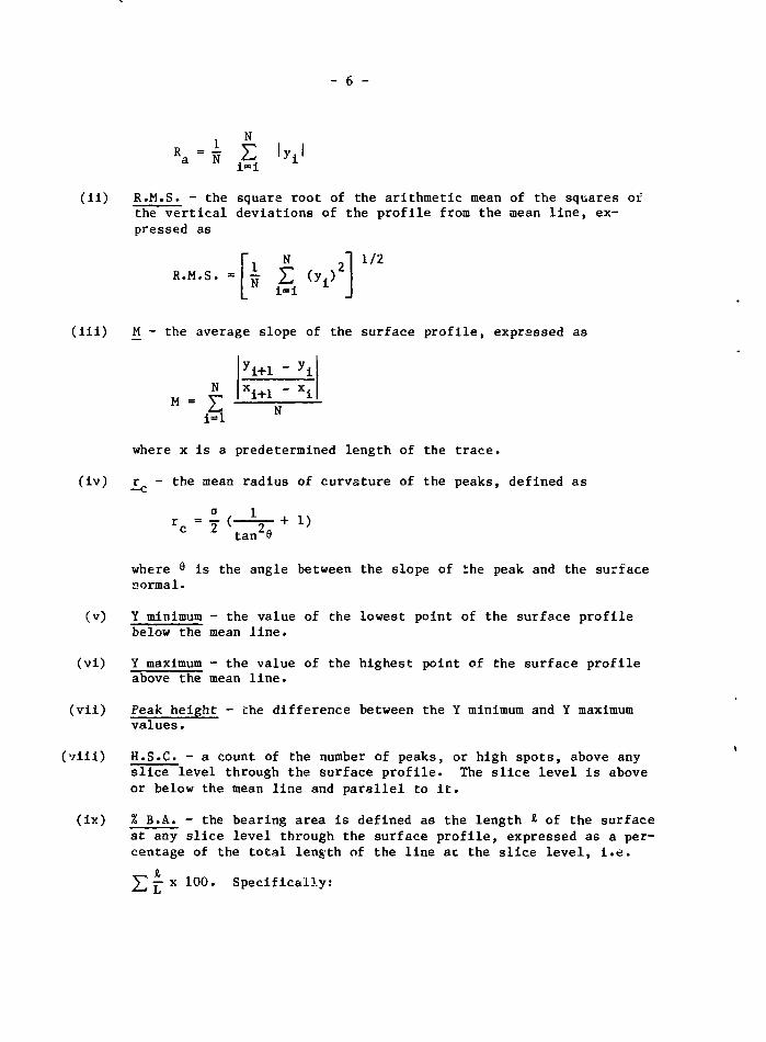
(i) R (also known as C.L.A. and AA) - the arithmetic average depar-ture of the surface profile above and below the mean line,expressed as

- 6 -

(ii) R.M.S. - the square root of the arithmetic mean of the squares ofthe vertical deviations of the profile from the mean line, ex-pressed as

(iii) tf - the average slope of the surface profile, expressed as

NM = T - iT4 Ki

itl N

where x is a predetermined length of the trace,

(iv) r - the mean radius of curvature of the peaks, defined as

arc = i 4

tan 9

where e is the angle between the slope of the peak and the surfacenormal.

(v) Y minimum - the value of the lowest point of the surface profilebelow the mean line.

(vi) Y maximum - the value of the highest point of the surface profileabove the mean line.

(vii) Peak height - the difference between the Y minimum and Y maximumvalues.

(viii) H.S.C. - a count of the number of peaks, or high spots, above anyslice level through the surface profile. The slice level is aboveor below the mean line and parallel to it.

(ix) % B.A. - the bearing area is defined as the length * of the surfaceat any slice level through the surface profile, expressed as a per-centage of the total length of the line at the slice level, i.e.

^ Specifically:

- 7 -

(x_ - x ) + (x, - x~) + (x - x )

% B.A. = - r ~ 2 L i -

where in this case the x values are the points where the slicelevel intersects the surface profile.

The data processing program is shown schematically in Figure 15.It consists of five separate routines or sub-programs:

1. Data collection.2. Data analysis initialization.3. Polynomial regression (to determine mean line through the data).4. Through-surface analysis.5. H.S.C. and B.A. curve plot.

The polynomial regression sub-program [4-8] determines the slopeand intercept coefficients of the mean line through each cut-off length datasample. The cut-off length is a fraction of the trace length selected toeliminate waviness from the analysis. The minimum and maximum Y values ofthe original data are then calculated, for verification purposes. The dataare stored on tape in array form for use in the through-surface analysis.

A polynomial of the form

Y = a + a. x , + + a x

is fitted to the X, Y data. Normal equations are formed and reduced by thesquare-root (Cholesky) method [4-8]. The profile is then normc.lized to amean line at 0 by

Yl = [Y - (mx + b)] sine

where m = slope;b = intercept;6 = arc tan (1/m) .

The effectiveness of the polynomial least-squares fit program isillustrated in Figure 16, where Figure 16(a) is a plot of the original dataand Figure 16(b) is a plot of the same profile normalized to a mean line at0. Note the magnification change.

The through-surface analysis continues by determining the Ymin.and Ymax. values for the normalized data and storing these in memory as anarray. The surface profile data are then converted to absolute values,integration is performed and the result assigned to a variable for accumu-lation for later determination of the R values. The absolute values of theprofile data are then squared, integration is performed and the result as-signed to a variable for accumulation for later determination of the R.M.S.value. Integration is performed using the trapezoidal rule:

- 8 -

Yo(l) = 0Yo(t) <= Yo(tfor t = 2, 3,

- 1)4 ..

+ 0 •5(Yl(t -N

where N is the number of elements in the array and Yl is the measuredheight.

When the data for all the cut-off samples have been processed, thearray containing the Ymin. and Ymax. values is scanned to find the minimumand maximum values for the entire profile. The C.L.A. and R.M.S. values forthe entire profile are then calculated and printed out for reference (seeTable 2).

To derive the H.S.C. and B.A. values, the slice level increment iscalculated by

Y9 lYlmin.j + |Ylmax.|N - 2

This ensures that the first and last H.S.C. values will be 0 and that theB.A. will range from 0 to 100% - the lowest and highest slice levels beingbelow and above the minimum and maximum values, respectively, by one slicelevel increment. A slice level at the mean line is assured by appropriatelysetting the first slice level as follows:

Y3 = [(integer (|Y"*n>l ) + 1) Y2]Y2

A threshold is set above which a peak or high spot must rise to becounted. We decided to set the threshold level at 0.0125 pn, half the totalbackground error range, as the majority of the background data were distrib-uted within that range. The threshold value is added to the first slicelevel. Data for the first cut-off sample are read, normalized to a meanline at 0, and stored in an array. The array is searched for the first ele-ment that crosses the threshold value. If the array values increase consec-utively, the crossing location is the first value that is equal to orgreater than the threshold value. If the values decrease consecutively, thecrossing location is the first value that is less than or equal to thethreshold value. If there is no crossing at a slice level below the meanline, the B.A. is set at 100%. If there is no crossing at a slice levelabove the mean line the B.A. is set at 0%. If the threshold is crossedbetween array values, the routine interpolates and returns a more precisevalue.

Both the rising and falling crossings are counted in accumulatingthe H.S.C. data. B.A. data are accumulated by subtracting the value of thelocation of the rising crossing from the value of the location of the fal-ling crossing and adding the results for each peak. If the first crossingis falling, the value is added to the B.A. count; if the last crossing isrising, the value is subtracted from the total number of data values and theresult added to the B.A. count. This process is carried out at each slicelevel on each sample and the data accumulated.

- 9 -

When the last cut-off sample has been processed, the crossingcounts for each slice are halved to provide the H.S.C. data, the % B.A.value for each slice is derived, and both are stored as the X-axis valuesfor the graph. The slice level values are stored as the Y-axis, values.Tan e and r values are calculated and stored, along with the otherparameters derived, for print-out from the plotting sub-program.

7. ACCURACY AND REPRODUCIBILITY

Calibration was carried out using the roughness standard suppliedby the manufacturer of the Talysurf 4 and a step of known height on a tung-sten carbide block. During the calibration procedure the R value was read,and a series of readings of H.S.C. and % B.A. were taken from the meter atthe mean line and at 10 slice levels above and below the mean line to con-struct a graph for comparison with the data system output.

Factors for magnification and voltage-to-height conversion for thesoftware program were arrived at by measuring the voltage difference forfull-scale deflection on the recorder graph at each magnification level anddividing the results into the representative full scale height. The voltagedifference at all magnification levels was 5.6005 V + 0.5 mV(+ 0.00928%).

To check overall accuracy, the measurement procedure was repeatedat magnifications of 500, 1000, 2500, 5000 and 20 000 using the 2.49 vmstep, and at 10 000, 20 000 and 50 000 using the 0.33 ym step. In the firstcase, the profile height values ranged from 2.4090 (in to 2.5031 \im, with anaverage of 2.4967 jim. Assuming 2.497 jim to be the correct height, the stepcan be measured to within! 0.006 pn (± 0.244%). In the latter case, theprofile height values ranged from 0.3251 to 0.3373 pm, with an average of0.3312 pm. Again, assuming 0.3312 ym to be the correct height, this stepcan also be measured to within ± 0.006 yni (± 1.842%).

To examine the reproducibility, a series of five consecutive mea-surements were taken on each of the Talysurf calibration standard steps andon the tungsten carbide calibration step. For the step measurements, 50values of the digitized data were averaged at each side of the step.

A profile was taken of the magnification calibration steps on theTalysurf standard and a plot of the profile output from the computer wascompared to the electrographic recorder output. A profile was taken of theC.L.A. roughness standard at a horizontal magnification of 100 and a plot ofthe profile output from the computer was compared to the recorder graph.The data were then processed to provide the surface parameters and a graphof H.S.C. and % B.A. These were compared to the original surface profilegraphs from the computer and recorder.

Comparing the results of five measurements on each of the calibra-tion steps, the greatest difference was 0.003 738 4 ^m. Reproducibility andaccuracy of measurement of the 0.33 ym step were therefore better than± 1.129% (± 0.374% of full scale) at the most sensitive range of 50 000magnification. The C.L.A. values for the five measurements on the standard

\

- 10 -

ranged from 0.8773 vm to 0.8879 urn, with an average value of 0.8821 urn,giving a reproducibility of 1.202% and an accuracy of + 0.544% (+ 0.096% offull scale) at 10 000 magnification.

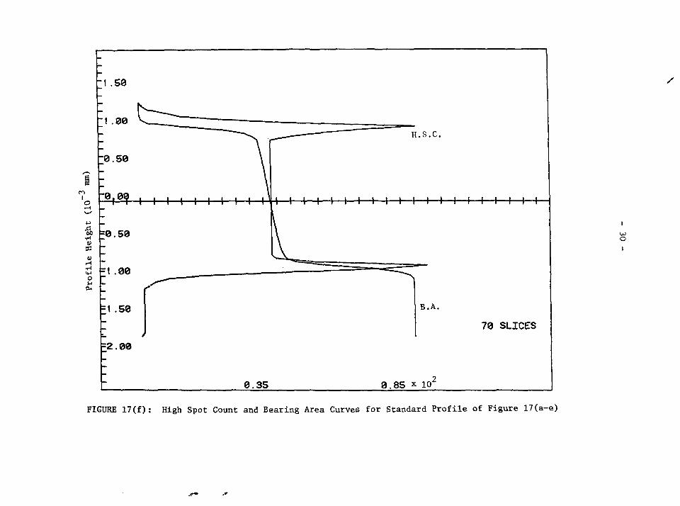
Figure 17 (a-f) shows five cut-off lengths of the roughness stan-dard profile plus the H.S.C. and B.A. curves. The surface parameters arelisted in Table 3. With the exception of one valley in the second cut-offlength (Figure 17(b)) the entire surface profile falls within the range- 1.13 jitn to + l.?G5 jim, giving a peak height of 2.415 jiin. Because that onevalley falls 0.64 ym below the next lowest valley, the peak height value of3.052 (in changes the H.S.C. and B.A. graphs significantly. This valleyprovides a distinctive focal point in the profile, illustrating how theH.S.C. and B.A. curves relate to the profile shape. These curves verify thethrough-surface analysis method. The almost ideal H.S.C. and B.A. curves inFigure 18 are the result of smoothing the surface at the peaks and valleys,and removing the deep valley from the second cut-off sample. The surfaceprofile, as shown in Figure 17, was repeated twice with no measurablechanges being observed, thus verifying that spikes on the peaks and valleyswere real and not the result of the stylus bouncing, a hardware problem or asoftware defect.

Comparison of surface profiles, as, for example, Figures 17(a),17(b) and 19, provides verification of the data reading frequency, verticaland horizontal magnification, cut-off length, H.S.C., % B.A. and the func-tion of the entire hardware and software system. The graphs show that thesurface profile is the same in all cases, i.e. that the height and width arethe same for each cut-off length of 0.75 mm.

TYPICAL RESULTS

We have applied the results of surface roughness measurements toseveral projects involving surfaces and their contact behaviour. Our maininterest is in its application to heat transfer at interfaces betweencontacting solids. The surface parameters are used in models that predictthe value of thermal contact conductance. These predictions are comparedwith experimental results to check the validity of the models.

This capability proved very useful in analyzing the results froman instrumented irradiation designed to measure the thermal contact conduc-tance between fuel pellets and cladding during irradiation [9]. Surface pa-rameters for both smooth and rough pellet surfaces are shown in Figures 20and 21, respectively, aloug with the H.S.C. and % B.A.

Parameters, such as the root mean square roughness, R.M.S., andthe mean surface slope, tan 8, were used in thermal conductance correlationsto predict the effects of surface texture on fuel-to-sheath heat transfer inthis experiment. The importance of accurate and reliable values for theseparameters is illustrated in Figure 22, which indicates that an increase insurface roughness has led to a significant increase in fuel temperature.

Use of surface roughness measurements has not been restricted toheat-transfer problems. It has proved useful, for example, in discerning

\

- l i -

the effects of electrochemical machining on the surface finish of Zr-2.5% Nbpressure tubes [10]. The profile measurements of Figures 23 and 24 indicatethat, in general, the electrochemlcally machined surfaces were rougher andwavier than surfaces prepared by the conventional fabrication methods.

9. FURTHER DEVELOPMENT

Additions to the system are planned to increase the resolution todetect very small changes in surface characteristics during an experiment.For example, the ability to measure small surface texture changes on theinner and outer surfaces of tubing is important to studies in reactorsafety. The additions planned are:

A high-resolution pick-up with a diamond stylus tip width of0.0012 mm and a stylus force of 50 mg, capable of resolving veryfine detail. This will be of great value in the examination ofcoated and uncoated specimens in thermal contact conductance ex-periments. The pick-up should be able to resolve the differencein characteristics of surfaces before and after coating and - withdevelopment of the right technique - provide a good approximationof coating layer thickness.

A 500 X horizontal magnification drive unit, which will enable thebest possible recording of the fine detail provided by the highresolution pick-up and permit the measurement of rougher surfacesusing the standard pick-up.

A reversible stylus, primarily for use in checking parallelism andwhich is also reversible to provide profiles of upper and lowersurfaces of a bore.

- A mass data storage device and extended memory to enable theprocessing of data from surface profiles at the resolution andmagnification of the high-resolution stylus and 500 X horizontalmagnification drive unit.

10. CONCLUSIONS

The surface measurement system described here provides measurementdata according to the standards set up for the Talysurf 4 profilometer, de-termines other significant surface parameters and produces a graph of H.S.C.and % B.A. with a high degree of accuracy.

The resolution and accuracy of the system are mainly dependentupon the total system noise, most of which is contributed by background vib-ration. Under prevailing operating conditions, the system is capable ofmeasuring a 0.10 \im step with an accuracy of better than ± 2.7%.

Single-trace measurements at a low traversing speed, together withan independent datum, minimize surface deformation and greatly improve the

\

- 12 -

accuracy of through-surface analysis. Relocation profilometry can be carriedout within 0.05 ym.

ACKNOWLEDGEMENTS

Thanks are due to Rank Taylor Hobson for drawings and specialtechnical data for the Talysurf 4; to Ray Thomas of Tektronix Canada Ltd. forhis continuing support and invaluable technical advice for the improvement ofsystem performance; to Ian Peggs, who initiated the surface measurementstudies and defined the project requirements; and to Mike Wfigbt for hisencouragement and contribution to this report.

REFERENCES

1. E.J. Abbot and F.A. Firestone, "Specifying Surface Quality", Mech.Eng. 55_, 569 (1933).

2. R.E. Reason, "The Measurement of Surface Texture", in Modern Work-shop Technology, Part II, Macmillan and Co. Ltd., London, 1970.

3. F.J. Hughes and I.D. Peggs, "An Exact Relocation Turntable for theTalysurf 4", Unpublished Whiteshell Nuclear Research EstablishmentReport, WNRE-213 (1981).

4. F.A. Graybill, An Introduction to Linear Statistical Models,Vol. 1, McGraw-Hill, New York, 1961.

5. R.W. Kopitzke, T.J. Boardman and F.A. Graybill, "Least SquaresPrograms - A Look at the Square Root Procedure", Amer. Statist.2£, 64 (1975).

6. S.H. Wilkinson, The Algebraic Eigenvalue Problem, Oxford Press,London, 1965.

7. Tektronix Inc., Plot 50: Statistics, Vol. 3, Beaverton, Oregon,1975.

8. F.A. Graybill, An Introduction to Matrices with Applications inStatistics, Wadsworth Publishing Co., Belmont, California, 1969.

9. M.H. Schankula and R.W. Mills, "In-Reactor Measurements ofFuel/Sheath Heat Transfer", Trans. Amer. Nuc. Soc. 27, 689 (1977).

10. D.W. Patterson, personal communication.

\

- 13 -

TABLE 1

SYSTEM NOISE MEASUREMENTS

a

b

c

d

Ymln.

(mm x 10~4)

-1.204

-0.2137

-0.0258

-0.3215

Ymax.

(mm x 10~4)

1.403

0.2009

0.0229

0.4229

PeakHeight

-4(mm x 10 )

2.635

0.4146

0.0487

0.7444

Ra

(um)

0.03134

0.0054

0.0003

0.0082

R«M • S •

(pm)

0.03918

0.0066

0.0005

0.0102

M

(tan 6)

0.0638

0.0109

0.0008

0.0146

c(ym)

4.0587

0.7897

0.01197

0.7817

a - background vibration, no flotation

b - background vibration, table floating

c - electrical noise, stylus suspended

d - total system noise, pick-up traversing optical flat

\

TABLE 2

PARAMETER LIST OUTPUT

Surface Characterization

REF:A038-SYS-VER/0-1/5/80:4:17.

SAMPLE DESCRIPTION: CLA STANDARD - TABLE FLOATING.

TRACE = 3.75 mm CUT-OFF K = 0.75 mm.

R value = 0.877832175227 m R.M.S. value - 0.8950400905113.

tan 6 = 0.145479210142

rc value - 1.63392081021 ym

DefinitionsR = centre line average roughnessR.M.S. = Root Mean Square average roughnessThese are defined as follows:

N

R = •£• R.M.S. =[*where y is measured from the mean line,tan 9 = average slope of the surface profile,r = mean peak radius of curvature.

TABLE 3

SURFACE PARAMETERS FOR Talysurf 4 STANDARD

Ymin. -

Ymax. -

Peak Height -

R -a

R.M.S. -

m(tan6) -

rc ~

-1

1

3

0

0

0

1

.767

.285

.052

.8778

.8950

.1460

.650

pm

nn

ym

um

\

- 15 -

Over a length of surface L, the centre line is a line drawn such thatthe sum of the areas embraced by the surface profile above the line isequal to the sum of those below the line.

Areas A+C+E+G+I = areas B+D+F+H+J+K

FIGURE 1: Definition of Centre Line

Y2Y3Y<

ij

!

>Y«

Ity

1

\y r

The C.L.A. value of the surface is the average height of the profileabove and below the centre line.

C.L.A.Y1+Y 2+--+Yi+—+Yn

where Yi is the height of the profile above or below the centre line atn equally spaced points along the surface. L is the sampling length.

FIGURE 2: Derivation of C.L.A.

\

- 16 -

AV

Mean Line

B Mean Line

Mid-height Line

C - —• Mid-height Line

Mean Line

D Mid-height andMean Line

FIGURE 3: Examples of Surface Profiles Showing Various Positions of the Mean Line

\

- 17 -

1 count no count 1 count I count 2 counts Total = 5 counts

SI ice Level

— — — Mean Line

traverse D , (A+B+C+D+E)Percentage bearing area = ^ x 100

start otraverseend

FIGURE 4: Measurement of Bearing Area and High Spot Count

Fi1teredProfile

AbbottF i restoneCurve

High SpotCurve

i—i—i n i iPercentage Counts perBearing Area Millimetre

FIGURE 5: Derivation of Abbott-Firestone Curve

OSCILLATOR MAGSWITCH

ELECTRONIC UNITMETER CUT-OFF SWITCH

AMPLIFIERAND

DEMODULATORFILTER

AVERAGEMETERDRIVE

TO DATA SYSTEM

PICK UP GEARBOX

RECORDER

STYLUS

00

I

FIGURE 6: Schematic Arrangement of Talysurf A Profilometer

\

- 19 -

o

u

\

- 20 -

FIGURE 8: Skid and Stylus Marks on Zircaloy-4 Specimens

- 21 -

LEGEND

A Datum attachment

B Datum support armlevelling device

C Datum levelling screw

D Quartz datum element

E Pick-up support arm

F Datum element

rotation control

G Pick-up noseplece

H Pick-up stylus

FIGURE 9: The 50.8 mm to Infinity Datum Element

- 22 -

43OS

ffi

Length (10 mm)

C6 , I 3.00 . 15.00

FIGURE 10(a>: Profile of Background Vibration with Table Resting

J3

cm

33

-_2.20

:2.50

'. .eeLength (10"1 mm)

1 3. ee , 5. © 7 . C8 E- 1 mm

FIGURE 10(b): Profile of Background Vibration with Table Floating

FIGURE 11: Air-Supported Granite Table

/

FIGURE 12: Exact Relocation Turntable

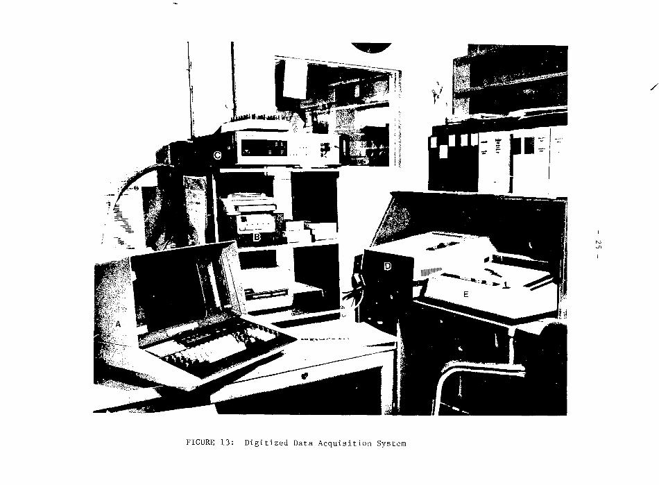
FIGURE 13: Digitized Data Acquisition System

BINARYLOADERROM

MATHPROCESSOR

SIGNALPROCESSOR]ROM

192 KMEMORYROM

FROM TALYSURF k DVM

ROM

EXPANDER

32 KGRAPHICCOMPUTER

QcTAPEDRIVE

GP-1B 1EEE-488 BUS

i

ho

FIGURE 14: Data Acquisition System Schematic

\

- 27 -

DETERMINE SLOPE AND INTERCEPT OF MEANLINE THROUGH DATA

NORMALISE PROFILE TO MEAN LINE AT 0.FIND Ymin AND Yraax VALUES. INTEGRATE |Y| VALUESFOR Ra AND IY2 I VALUES FOR RMS AVERAGES.

FIND Ymin AND Ymax AND CALCULATE Ra AND RMS FORFULL PROFILE. CALCULATE FIRST SLICE LEVEL.

SET FIRST SLICE LEVEL.

COUNT CROSSINGS AND NUMBER OF VALUES BELOW PROFILEFOR HSC AND BA GRAPH.

STORE SLICE LEVEL, HSC AND BA VALUES AND CALCULATETAN 6 AND T FOR ENTIRE PROFILE.

ICALL PLOT SUB-FROGRAK

FIGURE 15: Simplified Flow-Chart of Through-SurfaceAnalysis Sub-Program

\

O

00•H01X

- 28 -

FIGURE 16(a): Surface Profile - Original Data

01

Length (10 mm)

3.00 , 5.00

FIGURE 16(b): Surface Profile - Normalized Data

\

- 29 -

J..8B

je.sa

[e.se

ii-50

- - - -

1

L

1cng3- a

10

i

1

i

I 5 .

1

1*

7

CUT-OFF LENGTH

80 ,

J..09

¥l0Pl i )

13.50

^..58

2 00

1 | 00

I"

"B3

h do"68 , Is ee

' I I • 1 •' 1

80

(a) (b)

3 r d CUT-OFF i_CNGTl

-1

I I -BO • 1 3 8 9 • I 5.60 , I 7 . B8 ,

! i 0 O

|§.50

Li-se

| a

- i

-

-

L i - st3.

t

Ba

1-

o-

- 1

)1

1

5

-j

1

-

7

•

1 1 j 1 1 1 1 1 1 M [

* CUT-OFF LENGTH

(c) (d)

FIGURE 17(a-e): Talysurf Standard Profile (First Five Cut-off Lengths)

•"8,0

ID35

1 .58

1 .08

8.58

H.S.C.

r 0 ? i i i i

=8.58

= 1 .08

= 1 .58

=2.88

\—I—I—I—1 ) I—I—I—I—I—I—I—I—h-l-H-

B.A.

78 SLICES

0.35 8.85 x 10

oI

FIGURE 17(f): High Spot Count and Bearing Area Curves for Standard Profile of Figure 17(a-e)

•a

t .50

1 .00

0.50

H.S.C.

I I I I I I I I I I

=0.50

= 1 .00

= 1 .50

70 SLICES

0.35 0.85 x 10

FIGURE 18: Talysurf Standard High Spot Count and Bearing Area Curves - Smoothed Profile

25

20

15

JO

5

1st CUT-OFF SAMPLE 2nd CUT-OFF SAMPLE1.0 ym

0.1 ram

unu

n

IS5

-I 1 1 I I L j j I I

FIGURE 19: Recorder Graph of Two Sample Lengths, 0.75-mm Cut-Off

3.001

CO

O

4J

•a01SB

14-1

ou

2.00 —

1.00

0.00

-1.00

-2.00

-3,00

"4.00

/

-5.00'

R.M.S. Value = 0.66 ymTan 6 " 0.19

High Spot Count and Bearing AreaI

H—I I I

B.A.

SO Slices

0.00 0.50 i.oo xi a 2

FIGURE 20: Surface Parameters for Smooth Fuel Pellet

\

- 34 -

4.00

00•H

oM

2.00

0.00

-2.00

-4.00

R.M.S. Value = 1.64Tan 9 = 0.23

80 Slices

High Spot Count and Bearing Area I0.00 0.50 1.00 x 102

FIGURE 21: Surface Parameters for Rough Fuel Pellet

\

- 35 -

lOOOr

L. 900u3a1-v

| 800

3[X.

700

1 600

•is 400ij

- 200

±0

O 1.0 urn R.M.S.

O C.'JLUB

A 1 . 6 um R . M . S .

Element Internal Pressure (MPa)

10-5 10" 10-3 10-2 10-I 1.0 10

FIGURE 22: Effect of Gas Pressure on Fuel Temperature and Sheath Strain

- 36 -

2.00

1.00

0.00

-1.00

COIo

r -2.oo60

(1)

UPL,

-3.00

-4.00

-5.00

R.MTan

• S . Va lue = 0 .74 pm6 = 0 . 2 4

1 II I I I I I I I I I

I \) T \

I I0 5 10 15 20 25

High Spot Count and Bearing Area

0.00 0.50 1.00 xlO2

FIGURE 23: Surface Parameters for Pressure TubeWith As-Fabricated Surface

4.00 t

CM

OrH

Heig

ht

1P

rofi

le

3.

2

1

00

.00

.00

0.00

-1 .00

-2.00

"3.00

R.M.S. Value = 6.17 ymTan 6 = 0.43

60 Slices

High Spot Count and Bearing Area1

0.00 0.50 1.00 x 102

FIGURE 24: Surface Parameters for Pressure Tube With Electrochemically Machined Surface

ISSN 0067-0.36"' ISSN 0067-0367

I'n idemih individual di>cumenls in Ihe scries

we ha\e assigned an AHC'L- number to each.

Please refer to the AECL- number when

requesting additional copies of this document

from

Scientific Document Distribution Office

Atomic Energv of Canada Limited

Chalk River, Ontario. Canada

KOJ UO

Pnur identifier les rapports individuals faisam panic de cette

seric nous avons assigns' un numero AECL- a chacun.

Veuille/ faire mention du numero AECL -si vous

demande/ d'autres exemplaires de ce rapport

au

Service de Distribution des Documents Officiels

L'Energie Atomique du Canada Limitee

Chalk River. Ontario, Canada

KOJ 1JO

l'rue: S-4.(K) per copv nn\ : S-L00 par exemplaire