attachment c3-1.1: sediment distribution supporting...
TRANSCRIPT
Coastal Protection and Restoration Authority 450 Laurel Street, Baton Rouge, LA 70804 | [email protected] | www.coastal.la.gov
2017 Coastal Master Plan
Attachment C3-1.1: Sediment Distribution Supporting Information Report: Version II Date: May 2016 Prepared By: Alex McCorquodale (University of New Orleans), Gregg Snedden (USGS National Wetlands Research Center), Hongqing Wang (USGS National Wetlands Research Center), Brady Couvillion (USGS National Wetlands Research Center), Holly Beck (USGS National Wetlands Research Center), Ben Roth (Water Institute of the Gulf), and Eric White (Water Institute of the Gulf)
2017 Coastal Master Plan: Sediment Distribution Supporting Information
Page | ii
Coastal Protection and Restoration Authority
This document was prepared in support of the 2017 Coastal Master Plan being prepared by the Coastal Protection and Restoration Authority (CPRA). CPRA was established by the Louisiana Legislature in response to Hurricanes Katrina and Rita through Act 8 of the First Extraordinary Session of 2005. Act 8 of the First Extraordinary Session of 2005 expanded the membership, duties, and responsibilities of CPRA and charged the new authority to develop and implement a comprehensive coastal protection plan, consisting of a master plan (revised every five years) and annual plans. CPRA’s mandate is to develop, implement, and enforce a comprehensive coastal protection and restoration master plan. Suggested Citation: McCorquodale, J. A., Snedden, G., Wang, H., Couvillion, B., Beck, H., Roth, B. & White, E. (2016). 2017 Coastal Master Plan: Attachment C3-1.1 - Sediment Distribution Supporting Information. Version II. (pp. 1-102). Baton Rouge, Louisiana: Coastal Protection and Restoration Authority.

2017 Coastal Master Plan: Sediment Distribution Supporting Information
Page | iii
Table of Contents Coastal Protection and Restoration Authority ............................................................................................ ii 1.0 Introduction ............................................................................................................................................... 4 2.0 Sediment Processes in the Open Water Areas .................................................................................. 4 3.0 Sediment Deposition within Marsh Areas .......................................................................................... 26 4.0 Hurricane/storm-induced Sedimentation ......................................................................................... 46 5.0 Utilization of Remote Sensors and Techniques to Quantify Suspended Sediment ................... 72 5.1 Landsat .................................................................................................................................................... 72 5.2 Neural Network....................................................................................................................................... 80 5.3 MODIS, AVHRR, SeaWifs and Other Coarse Spatial, High Temporal Resolution Sensors ......... 81 6.0 Calibration/Validation of Suspended Sediment Using Remote Sensing .................................... 92 6.1 Potential Uses .......................................................................................................................................... 93 7.0 Simulating Spatial Patterns of Storm Sedimentation ....................................................................... 95 7.1 Spatial Patterns ....................................................................................................................................... 95 S .......................................................................................................................................................................... 95 7.2 Total Sediment Load ............................................................................................................................. 98 7.3 Spatial Distribution of Sediment .......................................................................................................... 99 8.0 Additional Literature Cited ................................................................................................................ 100

2017 Coastal Master Plan: Sediment Distribution Supporting Information
Page | 4
1.0 Introduction
The fate of mineral sediment in the coastal area involves: sediment sources, sediment transport within the coastal area, sediment transfer to and from the marsh areas and sedimentation processes within the marsh areas.
The purpose of this document is twofold: 1) to summarize the findings of the literature search on coastal sediment distribution to provide guidance for the development of conceptual integrated coastal model, and 2) to document several approaches to modeling which were considered by the sediment distribution team but not implemented in the final hydrology subroutine.
The literature survey was developed using the following topics:
• Sediment processes in the open water areas • Sediment processes in the marsh areas • The effects of hurricanes on the sedimentation processes • The use of remote sensing to indicate coast wide sediment responses to wind events
The specific approaches considered but not implemented were:
• Calibration/validation of suspended sediment using remote sensing • Assessing spatial patterns of sediment distribution by hurricanes
Citations considered during the literature review aspect of the work are listed within those sections. A list of additional references cited is provided at the end of this document.
2.0 Sediment Processes in the Open Water Areas
The open water areas of the Louisiana Coastal Area are generally shallow (depths in the range of 0.5 m to 5 m) and vary from freshwater to brackish and highly saline water. The 2012 Coastla Master Plan eco-hydrology model for the open water was based on the processes used in the ECOMSED (HydroQual 2002).
The literature herein will address the water column processes and the horizontal transport in the storage and channelized components of the coastal area.
The following summary provides a literature review of papers that discuss sediment distribution processes and formulae applicable to open water areas. Specific attention was given to the following items:
• Wind and wave induced processes • Sedimentation of silt and clay: flocculation • Sand transport
1. Booth, J. G., Miller, R. L., McKee, B. A., & Leathers, R. A. (2000). Wind-induced bottom
sediment resuspension in a microtidal coastal environment. Continental Shelf Research, 20(7), 785-806.
2017 Coastal Master Plan: Sediment Distribution Supporting Information
Page | 5
Summary
• Surface gravity waves are the primary mechanism for resuspension in shallow micro-tidal environments.
• Wind-induced wave equations are combined with wave theory.
o Wave equations developed for the formation and propagation of wind-induced waves developed by the USACE Coastal Engineering Research Center (CERC) were incorporated into this analysis.
o Variables include water depth, wind speed, and wind direction to predict resuspension.
• Study area is the Barataria Basin. • Satellite imagery is used to verify model results.
o Synoptic coverage of basin processes. o In this instance saturation radiance is the parameter that directly affects the study
of turbid waters via satellite.
• Material transport within the basin.
o Maximum transport times occur in fall and winter with the passage of cold front systems (southerly winds that precede the system push water into the basin, the subsequent northern winds drain the basin).
o Fluvial inputs are cut off by the existing levee system along the Mississippi River. o Freshwater input to the system is via precipitation. o Storm passages are the predominant mechanism that induces marsh sediment
deposition.
• 75% occurs as a result of winter storms (excluding tropical events in the Gulf of Mexico).
• The sediment source is largely from lakes and bays. • Equations
o When waves with wavelength (L) occur in a depth of water (d) such that d<L/2, wave motion can induce resuspension; therefore the critical wavelength is defined as Lc = 2d. Above this Lc value resuspension can be expected.
o Wavelength is related to wave period (T):
𝐿 = 𝑔𝑇2/2𝜋 where g is gravitational acceleration.
o The wave period can be predicted using wind velocity (U), wave fetch (F), wind
stress factor (UA), and 24-hour average resultant wind vectors such that:
𝑔𝑇/𝑈𝐴 = 0.2857(𝑔𝑔/𝑈𝐴2)1/3
o The wind stress factor is given by

2017 Coastal Master Plan: Sediment Distribution Supporting Information
Page | 6
𝑈𝐴 = 0.71�𝑈/𝑅𝑇 �
1.23
where RT is a boundary layer correction factor that is a function of the temperature difference between the air and water.1
• For a particular location:
o Dominant wind direction determines the fetch. o Water depth determines the critical wavelength. o Therefore substituting in the critical wavelength parameters provides a critical
wave period (Tc).
𝑇𝐶 = (4𝜋𝜋/𝑔)1/2
• By substitution the critical wind speed (Uc) is given
𝑈𝑐 = (1.2{4127(𝑇𝑐3/𝑔)}0.813)
• For the calculations performed, hourly wind data from National Data Buoy Center (NDBC) stations adjusted for the measurement height (10m).
• Summary of results provides an assessment of wind and resuspension seasonality.
2. Cózar, A., Gálvez, J. A., Hull, V., García, C. M., & Loiselle, S. A. (2005). Sediment resuspension by wind in a shallow lake of Esteros del Iberá (Argentina): a model based on turbidimetry. Ecological Modelling, 186(1), 63-76.
Summary
• Using wave theory, a daily spatial model of resuspension was built from simultaneous time series of hourly measurements of infrared nephelometric turbidity, wind speed and wind direction.
• The model was used to predict total suspended solids in another lake of the wetland. • The ecological effects of the resuspension could be summarized at three fundamental
levels.
o Resuspension works directly on the nutrients and pollutants dynamics. o Resuspension events modify significantly both attenuation and temporal
fluctuation of light in the water column.
• Hellestrom (1991) calculated that this effect would be sufficient to reduce primary productivity in a shallow Swedish lake by about 85%.
o Wind is considered one of the strongest factors influencing the zonation of aquatic vegetation. Even moderate wave heights (0.1–0.15 m) may cause
1 A value of 1.1 is suggested in the event that data are not available.
2017 Coastal Master Plan: Sediment Distribution Supporting Information
Page | 7
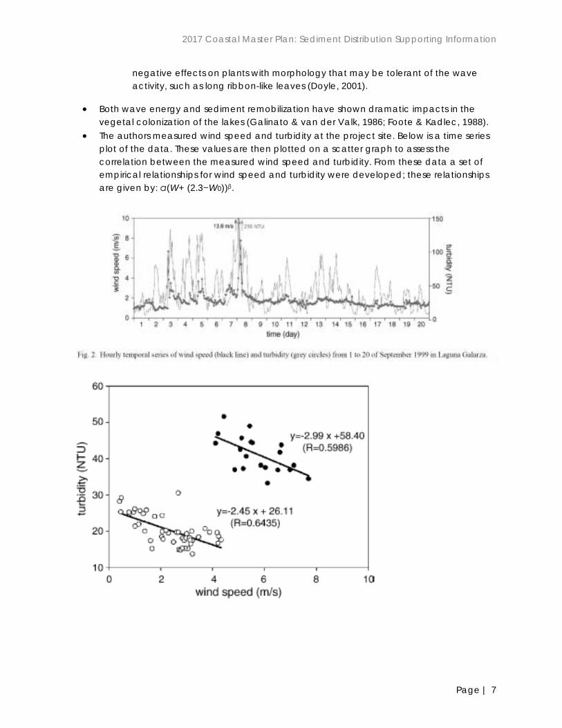
negative effects on plants with morphology that may be tolerant of the wave activity, such as long ribbon-like leaves (Doyle, 2001).
• Both wave energy and sediment remobilization have shown dramatic impacts in the vegetal colonization of the lakes (Galinato & van der Valk, 1986; Foote & Kadlec, 1988).
• The authors measured wind speed and turbidity at the project site. Below is a time series plot of the data. These values are then plotted on a scatter graph to assess the correlation between the measured wind speed and turbidity. From these data a set of empirical relationships for wind speed and turbidity were developed; these relationships are given by: α(W+ (2.3−W0))β.

2017 Coastal Master Plan: Sediment Distribution Supporting Information
Page | 8
• Model formulation
where: Lw = wavelength F = fetch W = wind speed
• Resuspension is induced for conditions where Lw ≥ 2D.

2017 Coastal Master Plan: Sediment Distribution Supporting Information
Page | 9
• A site-specific value for the critical wind velocity (W0) was determined based on the depth at the monitoring station. For this study W0 = 2.3 m/s
where: α(W+ (2.3−W0))β determines the turbidity from the actual wind speed, W (m/s), and the resuspension curve referred to the each value of W0; δ(W, W0) is a step-function that determines when the wind-induced wave begins to resuspend sediment,
δ=0 if W<W0 and δ=1 if W≥W0; 2.2 factor indicates the depth (m) where the wind-turbidity relation was originally determined. D is the depth (m) of the new site where it is applied. D is in the denominator because resuspended solids become more diluted when the water is deeper than 2.2 m depth.
3. Jin, K., & Ji, Z. (2004). Case Study: Modeling of Sediment Transport and Wind-Wave Impact in Lake Okeechobee. Journal of Hydraulic Engineering, 130(11), 1055-1067. doi:10.1061/(ASCE)0733-9429(2004)130:11(1055).
Summary
• Authors focus on cohesive sediments. • Wind-wave action induces sediment transport in the Lake Okeechobee system. • Development of the Lake Okeechobee environmental model (LOEM).
o Environmental Fluid Dynamics Code (EFDC). o 3-dimensional (2,126 cells 5 layers). o Modeled water column-sediment bed exchange per Ziegler and Nisbet (1994,
1995). o Similar approach to resuspension of cohesive sediments in ECOMSED: HydroQual
(2002); and Gailani et al. (1991).
• Cohesive Bed Equations (Jin and Ji 2004.)
o Deposition Flux.
𝐽𝑑 = �−𝑤𝑠𝑆𝑑
𝜏𝑐𝑑 − 𝜏𝑏𝜏𝑐𝑑
𝜏𝑏 ≤ 𝜏𝑐𝑑
0 𝜏𝑏 ≥ 𝜏𝑐𝑑
ws = Vertical Settling Velocity Sd = Sediment Concentration τb = Bed stress τcd = Critical stress for deposition2
2 Dependent on sediment and floc properties
2017 Coastal Master Plan: Sediment Distribution Supporting Information
Page | 10
o Erosion Flux
𝐽𝑟 = �𝜋𝑚𝑒
𝜋𝑑�𝜏𝑏 − 𝜏𝑐𝑒𝜏𝑐𝑒
�𝛼
𝜏𝑏 ≥ 𝜏𝑐𝑒
0 𝜏𝑏 < 𝜏𝑐𝑒
dme/dt = Surface erosion rate per unit bed surface area α = Site-specific parameter τce = Critical stress for surface erosion or resuspension
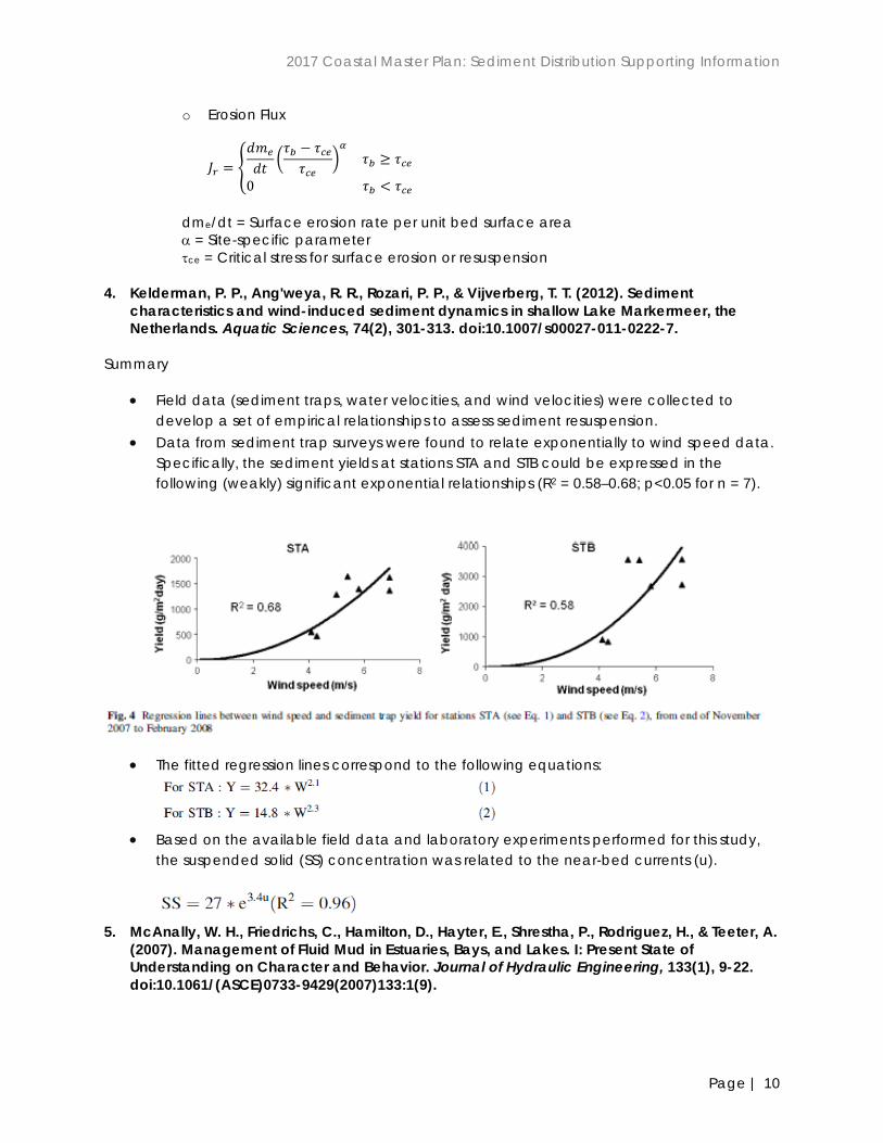
4. Kelderman, P. P., Ang'weya, R. R., Rozari, P. P., & Vijverberg, T. T. (2012). Sediment
characteristics and wind-induced sediment dynamics in shallow Lake Markermeer, the Netherlands. Aquatic Sciences, 74(2), 301-313. doi:10.1007/s00027-011-0222-7.
Summary
• Field data (sediment traps, water velocities, and wind velocities) were collected to develop a set of empirical relationships to assess sediment resuspension.
• Data from sediment trap surveys were found to relate exponentially to wind speed data. Specifically, the sediment yields at stations STA and STB could be expressed in the following (weakly) significant exponential relationships (R2 = 0.58–0.68; p<0.05 for n = 7).
• The fitted regression lines correspond to the following equations:
• Based on the available field data and laboratory experiments performed for this study,
the suspended solid (SS) concentration was related to the near-bed currents (u).
5. McAnally, W. H., Friedrichs, C., Hamilton, D., Hayter, E., Shrestha, P., Rodriguez, H., & Teeter, A.
(2007). Management of Fluid Mud in Estuaries, Bays, and Lakes. I: Present State of Understanding on Character and Behavior. Journal of Hydraulic Engineering, 133(1), 9-22. doi:10.1061/(ASCE)0733-9429(2007)133:1(9).

2017 Coastal Master Plan: Sediment Distribution Supporting Information
Page | 11
6. McAnally, W. H., Teeter, A., Schoellhamer, D., Friedrichs, C., Hamilton, D., Hayter, E., & Kirby, R. (2007). Management of Fluid Mud in Estuaries, Bays, and Lakes. II: Measurement, Modeling, and Management. Journal of Hydraulic Engineering, 133(1), 23-38. doi:10.1061/(ASCE)0733-9429(2007)133:1(23).
Summary
• Identifies properties of fluid mud.
o Typical bulk densities range from 1080 to 1200 kg/m3. o Silt and clay-sized particles less than 62.5 microns. o Considers the disaggregated particulate fraction not the floc (loosely bound
aggregate).
• Fluid mud formation and movement
o Settling zones: free settling, flocculation, hindered, and negligible
C = total fine sediment concentration Ws50 = free settling velocity aw, nw, bw, mw,= empirical settling coefficients C1 = 0.1 to 0.3 kg/m3 C3 = 2 to 5 kg/m3 C = depth-mean sediment concentration (mass/volume)
o In-text discussion regarding wave-induced fluid mud formation and transport.
Also discussed are gravity flows, shear flows, and vertical transport by entrainment.
• Cites research correlating salinity to fluid mud formation
o Kineke et al. (1996) study of the Amazon shelf found salinity stratification favors fluid mud formation.
• Advection of salinity at the bottom of the water column influences suspended sediment spatial distribution.
• The processes for forming the salinity front and fluid mud are interrelated.
o Both salinity and temperature within fluid mud layers are typically different from the remainder of the water column.
7. Mikeš, D., & Manning, A. (2010). Assessment of Flocculation Kinetics of Cohesive Sediments from the Seine and Gironde Estuaries, France, through Laboratory and Field Studies. Journal of Waterway, Port, Coastal and Ocean Engineering, 136(6), 306-318. doi:10.1061/(ASCE)WW.1943-5460.0000053

2017 Coastal Master Plan: Sediment Distribution Supporting Information
Page | 12
Summary
• Floc size and settling velocity are key parameters for modeling sediment in estuaries.
o Floc settling and porosity increases with growth (Stoke’s Law), whereas density decreases.
o Parameters assessed
• Salinity, Suspended Particulate Matter (SPM) concentration, turbulence length scale, material composition, and time
• Micro- and macroflocs.
o Microflocs form in the river system and macroflocs form within the estuarine system.
o Macroflocs are important to sediment fate in the estuary due to the difference in settling rates.
o Microfloc mean size ranges from 25 to 50 µm and the settling velocity ranges from 0.001 to 1 mm/s.
o Macroflocs are typically larger than 160 µm in diameter and the settling velocity is generally between 1 and 5 mm/s but can reach 15 mm/s.
• Salinity and Sediment Concentration are key factors.
o Macrofloc formation occurs at a specific point in the estuary near the threshold salinity concentration.
o Threshold salinities vary widely 0.1 to 20 Practical Salinity Unit (PSU). o Macrofloc diameter size increases with sediment concentration up to an
optimum value, which ranges from 50 to 20,000 mg/L.
• Time and turbulence also affect mean floc diameter.
o R2 = 0.77 for correlation between turbulence and mean diameter. o Floc size also tends to increase with extended residence time (e.g., time between
tidal cycles).
• Site specific values for Seine and Gironde estuaries are included.
8. Pandoe, W. W., & Edge, B. L. (2008). Case Study for a Cohesive Sediment Transport Model for Matagorda Bay, Texas, with Coupled ADCIRC 2D-Transport and SWAN Wave Models. Journal of Hydraulic Engineering, 134(3), 303-314. doi:10.1061/(ASCE)0733-9429(2008)134:3(303).
Summary
• Study used a coupled version of ADCIRC and SWAN for the hydrodynamics and waves, respectively.
• Depositional flux rate follows van Rijn (1993):

2017 Coastal Master Plan: Sediment Distribution Supporting Information
Page | 13
with: ws=sediment settling velocity (m/s); τcd=critical bed shear stress for deposition and is estimated from laboratory tests to be between 0.05 and 0.15 N/m2 (van Ledden, 2003).
• The model used to estimate the erosion flux rate (E) expressed as dry mass of material
eroded per unit area per unit time (kg m−2 s−1) as a function of shear stress.
o Erosion flux formulation follows Partheniades (1990).
where: me=experimental/site-specific erosion constant for which Whitehouse et al. (2000) suggested a value of between me=0.0002 and 0.002 kN−1 s−1; τb=bed shear stress; and τce=critical bed shear stress for erosion around 0.1–0.6 N/m2, but it should not exceed 1.0 N/m2. No sediment interactions are considered in the model.
• The bed shear stresses under combined waves and currents are determined from an
addition of the wave-alone and current-alone stresses, which Whitehouse et al. (2000) formulate as follows:
in which: τb is given by a vector addition of τmean and τw; and φ=angle between wind and current vectors measured counter clockwise from current vector axis. τc and τw=bottom shear stresses, which would occur due to the current-alone and to the wave-alone, respectively.
• ADCIRC model setup allows for adjustment of critical erosion and deposition. This study
found the following values for the adjustable model parameters: ws =0.1 mm/s, me=0.0007 kN−1 s−1, τcd=0.10 N/m2, and τce =0.40 N/m2.

2017 Coastal Master Plan: Sediment Distribution Supporting Information
Page | 14
9. Teeter, A. M. (2002). Sediment transport in wind-exposed shallow, vegetated aquatic systems (Doctoral dissertation, Oregon State University).
Summary
• Presents evaluation of two model formulations: single and multiple grain classes.
o Single grain class models with simultaneous erosion and deposition are found to represent resuspension better than mutually exclusive models (i.e., steady state experiments do not show equivalence between these processes).
• Model calculates vertical gradients only.
o Sediment/water interface. o Erosion and deposition fluxes are calculated and mass conservation is solved for
each grain class. o Mass conservation equation:
H = water depth C = depth-mean sediment concentration (mass/volume) t = time E = erosion flux F = depositional flux gs = grain size class
o Near bed concentration Cb (used to calculate F).
Pe = Peclet number = HWs/Kz Ws = settling velocity Kz = 0.067U*H U* = friction velocity P =-depositional probability C = depth-mean sediment concentration (mass/volume)
o Erosion flux depends on: 1) erosion threshold of cohesive fraction and 2) erosion
threshold of silt fraction.
gs = 1 = cohesive fraction τ = bed shear stress τce = erosion threshold
2017 Coastal Master Plan: Sediment Distribution Supporting Information
Page | 15
** τ< τce no sediments are eroded ** ** critical shear stress for erosion is estimated by a power law depending on cohesive fraction concentration in the bed layer exposed to flow** ** erosion rate parameter M is based on Lee and Mehta (1994)**
o Additional equations are provided for
• Proportionality of erosion for silt to clay fraction. • Bed layer consolidation, thickness, hindered settling rate, and
concentration. Ribberink, J. S., van der Werf, J. J., O'Donoghue, T., Buijsrogge, R. H., & Kranenburg, W. M. (2013). Practical sand transport formula for non-breaking waves and currents. Coastal Engineering, 7626-42. doi:10.1016/j.coastaleng.2013.01.007.
Summary
• Semi-unsteady approach following “half-cycle” concept from Dibajnia & Watanabe (1992).
• Valid application for rippled bed and sheet-flow conditions; oscillatory flow and surface wave conditions.
• Phase lag and flow acceleration accounted for in formula. • Parameterization based on lab experiments. • Additional model required for sediment in suspension above bed/sheet-flow layer. • Non-Dimensional Net Transport Rate.
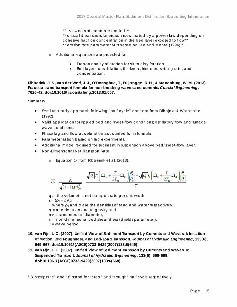
o Equation 13 from Ribberink et al. (2013).
qs = the volumetric net transport rate per unit width s = (ρs – ρ)/ρ
where ρs and ρ are the densities of sand and water respectively, g = acceleration due to gravity and d50 = sand median diameter; Ө = non-dimensional bed shear stress (Shields parameter), T = wave period
10. van Rijn, L. C. (2007). Unified View of Sediment Transport by Currents and Waves. I: Initiation
of Motion, Bed Roughness, and Bed-Load Transport. Journal of Hydraulic Engineering, 133(6), 649-667. doi:10.1061/(ASCE)0733-9429(2007)133:6(649).
11. van Rijn, L. C. (2007). Unified View of Sediment Transport by Currents and Waves. II: Suspended Transport. Journal of Hydraulic Engineering, 133(6), 668-689. doi:10.1061/(ASCE)0733-9429(2007)133:6(668).
3 Subscripts “c” and “t” stand for “crest” and “trough” half cycle respectively.

2017 Coastal Master Plan: Sediment Distribution Supporting Information
Page | 16
12. van Rijn, L.C. (2013). Simple General Formulae for Sand Transport in Rivers, Estuaries and Coastal Waters. Website: www.leovanrijn-sediment.com.
Summary
• Includes formulae and discussion regarding transport induced by currents in river and coastal areas.
• Describes the recalibration of the suspended transport model TR2004. • Suspended sand transport in river and tidal flow conditions.
o Size classes 60-100, 100-200, 200-400, and 400-600 µm o Depth 1-15m
𝑞𝑠 = �𝜋𝑟𝑒𝑟 𝜋50⁄ �2(𝑢 − 𝑢𝑐𝑟)3 o qs = suspended transport (kg/s/m) o d50 = median grain size (m) o dref = reference grain size (0.0003m) o u = depth averaged velocity (m/s) o ucr = critical depth averaged velocity (0.25 m/s)
• Coastal suspended sand transport current and wave conditions.
o Transport is dependent on relative wave height (Hs/h); especially for velocities ranging 0.1-0.6 m/s.
o Waves effectively stir sand into water column; however, this effect is lessened with increased currents.
• Mixing coefficient for combined steady and oscillatory flow (see van Rijn [2007] for full parameter descriptions).
𝜀𝑠,𝑐𝑐 = ��𝜀𝑠,𝑐�2 + �𝜀𝑠,𝑐�
2�0.5
o εs,w = wave-related mixing coefficient (m2/s). o εs,c = φdβcεf,c = current-related mixing coefficient due to main current (m2/s).
• Near bed concentration calculation is a function of particle size and flow (see van Rijn [2007] for full parameter descriptions); “specifies the sediment concentration at a small height above the bed (or fluid mud bed)”.
o ca = reference volume concentration o pclay = percent clay o fsilt = silt factor = dsand/d50
2017 Coastal Master Plan: Sediment Distribution Supporting Information
Page | 17
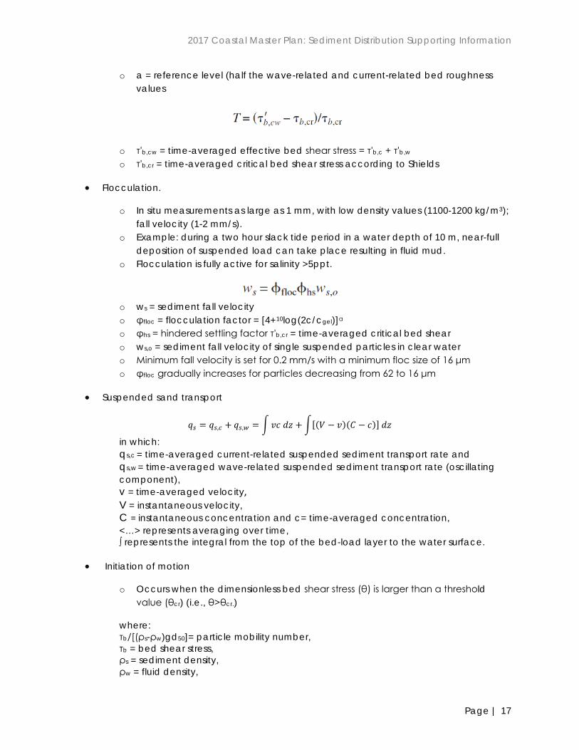
o a = reference level (half the wave-related and current-related bed roughness values
o τ'b,cw = time-averaged effective bed shear stress = τ'b,c + τ'b,w o τ'b,cr = time-averaged critical bed shear stress according to Shields
• Flocculation.
o In situ measurements as large as 1 mm, with low density values (1100-1200 kg/m3); fall velocity (1-2 mm/s).
o Example: during a two hour slack tide period in a water depth of 10 m, near-full deposition of suspended load can take place resulting in fluid mud.
o Flocculation is fully active for salinity >5ppt.
o ws = sediment fall velocity o φfloc = flocculation factor = [4+10log(2c/cgel)]α o φhs = hindered settling factor τ'b,cr = time-averaged critical bed shear o ws,o = sediment fall velocity of single suspended particles in clear water o Minimum fall velocity is set for 0.2 mm/s with a minimum floc size of 16 μm o φfloc gradually increases for particles decreasing from 62 to 16 μm
• Suspended sand transport
𝑞𝑠 = 𝑞𝑠,𝑐 + 𝑞𝑠,𝑐 = �𝑣𝑣 𝜋𝑑 + �[(𝑉 − 𝑣)(𝐶 − 𝑣)] 𝜋𝑑
in which: qs,c = time-averaged current-related suspended sediment transport rate and qs,w = time-averaged wave-related suspended sediment transport rate (oscillating component), v = time-averaged velocity, V = instantaneous velocity, C = instantaneous concentration and c= time-averaged concentration, <…> represents averaging over time, ∫ represents the integral from the top of the bed-load layer to the water surface.
• Initiation of motion
o Occurs when the dimensionless bed shear stress (θ) is larger than a threshold value (θcr) (i.e., θ>θcr.)
where: τb/[(ρs-ρw)gd50]= particle mobility number, τb = bed shear stress, ρs = sediment density, ρw = fluid density,

2017 Coastal Master Plan: Sediment Distribution Supporting Information
Page | 18
d50 = median sediment diameter. o θcr depends on conditions near the bed; hydraulic conditions can be described
using the Reynolds number Re* = u*d/ν. o Shield’s relationship is given in the following figure using θcr and the Reynolds
number.
• Effects of salinity.
o High-density salt wedge near the bed creates a significant density gradient o This stratification serves to dampen turbulent flows. o Modeling this dampening effect can be accomplished by applying a factor
related to the Richardson-number (Ri).
𝜀𝑟 = 𝜙𝜀𝑟,𝑜 where εf,o is the fluid mixing coefficient in fresh water φ is a function of Ri and is equal to the damping factor (<1) after Munk-Anderson (1948)
𝜙 = (1 + 3.3Ri)−1.5 o Ri is the local Richardson number o This relationship does not provide realistic results for the cases where damping
effects are high.
• Effects of mud.
o Sand-mud mixtures can display different behavior depending on the dominant particle size.
2017 Coastal Master Plan: Sediment Distribution Supporting Information
Page | 19
• If the mud fraction (sediment < 0.05 mm) is >0.3 the mixture behaves with cohesive properties.
• If the sand fraction is >0.7 the mixture behaves with non-cohesive properties.
• Cohesive and non-cohesive mixtures can be related by the critical mud content, pmud,cr.
• Clay fraction (<0.005 mm) is important in this relationship. o Cohesive properties dominate when clay fraction is 5-10%.
• For a clay-mud ratio of ½ to ¼ (natural mud beds) critical mud content will range from 0.2 to 0.4.
• If mud content is less than the critical value then the mixture can be assumed to be homogeneous and non-cohesive where sand erosion is the dominant mechanism.
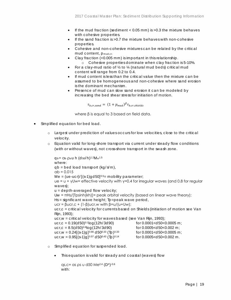
• Presence of mud can slow sand erosion it can be modeled by increasing the bed shear stress for initiation of motion.
𝜏𝑏,𝑐𝑟,𝑠𝑠𝑠𝑑 = (1 + 𝑝𝑚𝑚𝑑)𝛽𝜏𝑏,𝑐𝑟,𝑠ℎ𝑖𝑒𝑖𝑑𝑠
where β is equal to 3 based on field data.
• Simplified equation for bed load.
o Largest under prediction of values occurs for low velocities, close to the critical velocity.
o Equation valid for long-shore transport via current under steady flow conditions (with or without waves), not cross-shore transport in the swash zone.
qb= αb ρs u h (d50/h)1.2Me1.5 where: qb = bed load transport (kg/s/m), αb = 0.015 Me = (ue-ucr)/[(s-1)gd50]0.5= mobility parameter; ue = u + γUw= effective velocity with γ=0.4 for irregular waves (and 0.8 for regular waves); u = depth-averaged flow velocity; Uw = πHs/[Tpsinh(kh)]= peak orbital velocity (based on linear wave theory); Hs = significant wave height; Tp=peak wave period, ucr = βucr,c + (1-β)ucr,w with β=u/(u+Uw); ucr,c = critical velocity for currents based on Shields (initiation of motion see Van Rijn, 1993); ucr,w = critical velocity for waves based (see Van Rijn, 1993); ucr,c = 0.19(d50)0.1log(12h/3d90) for 0.0001<d50<0.0005 m; ucr,c = 8.5(d50)0.6log(12h/3d90) for 0.0005<d50<0.002 m; ucr,w = 0.24[(s-1)g]0.66 d500.33 (Tp)0.33 for 0.0001<d50<0.0005 m; ucr,w = 0.95[(s-1)g]0.57 d500.43 (Tp)0.14 for 0.0005<d50<0.002 m.
o Simplified equation for suspended load.
• This equation is valid for steady and coastal (waves) flow
qs,c= αs ρs u d50 Me2.4 (D*)-0.6 with:

2017 Coastal Master Plan: Sediment Distribution Supporting Information
Page | 20
qs,c = suspended load transport (kg/s/m); h = water depth, d50 = particle size (m), D* = d50[(s-1)g/ν2]= dimensionless particle size, αs = 0.012 (coefficient)4, s = ρs/ρw=relative density, ν = kinematic viscosity, Me = (ue-ucr)/[(s-1)gd50]0.5= mobility parameter (see bed load equation above), ue = effective velocity (see bed load equation above), ucr = critical depth-averaged velocity for initiation of motion (see bed load equation above).
• Application of the simplified equations.
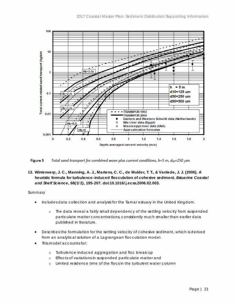
o The detailed TR2004 model (Van Rijn 2007) was used to compute the total sand transport rates (bed load plus suspended load transport) for a depth of 5 m and a median size of d50= 250 μm (d10= 125 μm, d90= 500 μm).
o The wave height was varied in the range of 0 to 3 m and wave periods in the range of 5 to 8 s. The wave direction is assumed to be normal to the coast, whereas the current is assumed to be parallel to the coast (ϕ=90o). The temperature is 15 degC and the salinity is 0 (fluid density= 1000 kg/m3).
o The total load transport (bed load + suspended load) results of the TR2004 model are shown in the figure below together with earlier results of the TR1993 model (Van Rijn, 1993) for the same parameter range. Some measured data of rivers and estuaries are also shown.
4 The original αs coefficient is αs = 0.012 (Van Rijn 1984). The most realistic variation range is αs =0.008 to 0.012. The best value matching the results of the detailed TR2004 results is αs =0.008 (see Figure in text).
2017 Coastal Master Plan: Sediment Distribution Supporting Information
Page | 21
13. Winterwerp, J. C., Manning, A. J., Martens, C. C., de Mulder, T. T., & Vanlede, J. J. (2006). A
heuristic formula for turbulence-induced flocculation of cohesive sediment. Estuarine Coastal and Shelf Science, 68(1/2), 195-207. doi:10.1016/j.ecss.2006.02.003.
Summary
• Includes data collection and analysis for the Tamar estuary in the United Kingdom.
o The data reveal a fairly small dependency of the settling velocity from suspended particulate matter concentrations, consistently much smaller than earlier data published in literature.
• Describes the formulation for the settling velocity of cohesive sediment, which is derived from an analytical solution of a Lagrangean flocculation model.
• This model accounts for:
o Turbulence-induced aggregation and floc break-up o Effects of variations in suspended particulate matter and o Limited residence time of the flocs in the turbulent water column

2017 Coastal Master Plan: Sediment Distribution Supporting Information
Page | 22
• Full description of variables is given in the text; this method, as presented, is highly parameterized. However the formulation and the authors’ findings may provide some insight.
• Resuspension by tidal currents and wind waves contribute to suspended matter.
o Observed that fine grained sediments were being resuspended from the shallow portions of San Francisco Bay and transported to deeper areas during the windier summer months. This process is sometimes referred to as focusing.
o Observed that wind wave resuspension is an important agent during high wind and rough seas, however, he also noted that high storm concentrations of suspended sediment were dissipated within a few days.
o Felt that wave resuspension of estuarine sediments could cause significant variation in the observed daily cycle of particulate matter flowing through estuaries.
o Study implies that although shallow water resuspension occurs with low amplitude waves, the sediments usually settle out very rapidly unless the water is rising upward and landward as it does on a flooding tide.
o In the case of the ebb tide, the water column is settling down and off the tidal flat. This may act to quickly redeposit more of the coarse sediment and weaken the relationship between wave height and resuspension.
o Indicates less resuspension at deeper waters with a given wave height. o Suspended sediment concentrations appear to be linearly predictable on the
flooding tide for shallow waters and low amplitude waves. o In less than 24 hours after wave resuspension most sediment appears to have
settled out or have been transported elsewhere.
14. Erm, A., Alari, V., & Kask, J. (2011, March). Resuspension of sediment in a semi-sheltered bay due to wind waves and fast ferry wakes. Boreal Environmental Research, 16, Suppl A, pp. 149-163.
Summary
• Anthropogenic resuspension plays a key role in the western part of Tallinn Bat during relatively calm spring and summer seasons.
• The near bottom orbital velocities generated daily by fast ferries’ wakes are equivalent to those induced by wind waves excited by at least 18 m/s southwestern winds and 12 m/s northwestern winds.
• About 400 kg of sediment is resuspended and carried away from each meter of coastline annually.
• Sediment resuspension events alter the concentration of dissolved phosphorus, with suspended solids acting either as its sink or source.
2017 Coastal Master Plan: Sediment Distribution Supporting Information
Page | 23
• Light attenuation also changes with the variations of the concentrations of suspended solids.
• Alterations in the sediment resuspension regime may also cause changes in the bottom topography.
• It may be concluded that resuspension of sediment at the measurement site is due to fast ferry wakes rather than wind waves.
• Concerning sediment flux, on the average, the seaward flux was 1.3 times as large as the shoreward one.
• The absolute majority of resuspension events were caused by ship wakes which induced resuspension higher as induced wind waves about 50 times at the .2 m level and about 200 times at the .5m level from the sea bed.
15. Kelderman, P., De Rozari, P., Mukhopadhyay, S., & Ang'weya, R. O. (2012). Sediment dynamics in shallow Lake Markermeer, The Netherlands: field/laboratory surveys and first results for a 3-D suspended solids model. Water Science and Technology, 66 (9), 1984-1990.
Summary
• This study took place on the shallow Lake Markermeer in the Netherlands (680 km2 , 90% depth between 2 and 5 m).
• Resuspension rates for the lake were very high, 1,000 g/m2 day as an annual average, leading to high suspended solids contents, due to the large lake area and its shallowness (high Dynamic Ratio).
• A 3-D model was set up using Delft 3-D. • Sediment characteristics, water depth, and fetch are main determinants for sediment
distribution patterns. • The research took place over 4 months and comprised of the following: taking an
inventory of major sediment characteristics at 50 stations; sediment traps field survey at two permanent stations; preliminary laboratory sediment resuspension experiments; set-up and first results of the 3-D lake water quality SS model.
• Taken into account were two different layers of bottom sediments: a thin, very “fluffy” layer prone to resuspension under already moderate wind conditions, and a more compact sediment layer.
• Sediment yield of 995 g/m2 day was derived. • Sediment resuspension started off at 0.5-0.7 cm/s. • For higher near-bed currents, an exponential increase could be observed with values up
to 500-3,500 mg SS/L for a velocity of 1.3 cm/s. • An exponential relationship between SS content (mg/L) and near-bed velocity C (cm/s)
was estimated: SS=27 x e3.4*C (with an R2=.96). • Using the 3-D model, a reduction of more than 80% of SS contents, and 30-50% reduction
of near bed currents was found in the case of placing artificial wetlands near the center of the lake. This reduced wind fetches by a factor of 2.
• Another possible measure for SS reduction would be the construction of large deep pits in the lake serving as final sedimentation basis for resuspended sediment material.

2017 Coastal Master Plan: Sediment Distribution Supporting Information
Page | 24
• Conclusion: a substantial reduction in lake water turbidities can only be brought about by reducing effecting wind fetches, thus reducing near-bed currents.
16. Blom, G., & Aalderink, R. H. (1998). Calibration of three resuspension/sedimentation models. Water Science Tech, 37 (3), 41-49.
Summary
• Three resuspension and sedimentation models from Blom, Lick & Partheniades & Krone, are calibrated and evaluated on data from flume experiments with sediments from Lake Ketal and in situ suspended solids measurements.
• Phosphorous has a strong tendency to associate with particulate material and large pools tend to accumulate in lake bottoms.
• Wind induced waves usually are the dominant driving force for sediment resuspension • Many models for resuspension and sedimentation are empirical but this study focuses on
models which are largely theoretically based. In these models, the resuspension flux is directly related to the forces at the water-sediment interface, caused by wind-induced waves.
• The sedimentation flux is equal or proportional to the fall velocity of the particles and the suspended solids concentration.
• Resuspension can be related to the orbital velocity at some distance near the sediment-water interface or the shear stress at the bottom surface.
• Sedimentation is described as a function of the bottom shear stress or related to the concentration and fall velocity only.
• Parameter values in resuspension and sedimentation models are related to particle size and density (distribution), sediment characteristics (cohesiveness).
• When horizontal transport by advection and dispersion can be neglected and vertical gradients in the suspended solids concentration are absent, the suspended solids dynamics can be described with:
• 𝛿𝐶𝛿𝛿
= ℎ−1(Φ𝑟 −Φ𝑠); in which C is the depth averaged suspended solids concentration (gm-
3), h is the depth (m), Φr is the resuspension flux (gm-2s-1) and Φs is the sedimentation flux (gm-2s-1).
Three models are discussed and presented: • Blom: in this model the resuspension flux is a function of the orbital velocity:
o Φ𝑟 = 𝐾𝐵�𝑢𝑏 − 𝑢𝑏,𝑐𝑟�; 𝑖𝑖 𝑢𝑏 > 𝑢𝑏,𝑐𝑟 o Φ𝑟 = 0; 𝑖𝑖 𝑢𝑏 ≤ 𝑢𝑏,𝑐𝑟 o 𝐾𝐵 is a resuspension constant (gm-3), 𝑢𝑏 is the maximal orbital velocity induced by
waves (ms-1) directly above the sediment surface and 𝑢𝑏,𝑐𝑟 is the minimal (critical) orbital velocity required for resuspension (ms-1).
• Lick (a): Φ𝑠 = 𝑤𝑠(𝐶 − 𝐶𝑏)

2017 Coastal Master Plan: Sediment Distribution Supporting Information
Page | 25
o in which 𝑤𝑠 is the fall velocity (ms-1) and 𝐶𝑏 is a “background” concentration of non0settling suspended material (gm-3). The fall velocity of particles is a function of their size and density.
• Lick (b): Φ𝑟 = 𝐾𝐿�𝜏𝑏−𝜏𝑏,𝑐𝑐�𝜏𝑏,𝑐𝑐
; 𝑖𝑖 𝜏𝑏 > 𝜏𝑏,𝑐𝑟
o Φ𝑟 = 0; 𝑖𝑖 𝜏𝑏 ≤ 𝜏𝑏,𝑐𝑟 o in which 𝐾𝐿 is the resuspension constant (gm-2s-1), 𝜏𝑏 is the maximal bottom shear
stress induced by the orbital velocity (Pa), and 𝜏𝑏,𝑐𝑟 is the minimal (critical) bottom shear stress.
Partheniades and Krone: in this model the sedimentation flux is a function of the bottom shear stress. It is constrained by a maximal (critical) bottom shear stress, which is by definition, lower than the critical shear stress for resuspension of sediments. Thus resuspension and sedimentation cannot occur simultaneously:
• Φ𝑠 = 𝑤𝑠�1 − 𝜏𝑏/𝜏𝑐𝑟,𝑠� ∗ (𝐶 − 𝐶𝑏) ; 𝑖𝑖 𝜏𝑏 ≤ 𝜏𝑐𝑟,𝑠 • Φ𝑠 = 0 ; 𝑖𝑖 𝜏𝑏 > 𝜏𝑐𝑟,𝑠 • in which 𝜏𝑐𝑟,𝑠 is the maximal (critical) shear stress for sedimentation (Pa) • The maximal orbital velocity near the bottom was obtained from (Phillips, 1966)
calculated from the bottom shear stress formula: • 𝜏𝑏 = 0.5𝜌𝑐𝐶𝑟𝑢𝑏2 • in which 𝐶𝑟 is a dimensionless friction factor, taken here as .004 used in (Sheng & Lick,
1979). 𝜌𝑐 is the density of water (kgm-3)
All three models produce, after calibration, a good reconstruction of the data set from the flume experiment. Although the differences in the model fit are not significant, Lick’s model resulted in the best fit.
17. Lee, C., Schwab, D. J., & Hawley, N. (2005). Sensitivity analysis of sediment resuspension parameters in coastal area of southern Lake Michigan. Geophysical Research, 110.
Summary
• Model sensitivity analysis was performed to identify and compare quantitatively the important resuspension parameters in the coastal area of southern Lake Michigan.
• A one-dimensional resuspension and bed model capable of dealing with the type of mixed sediments (fine-grained+sand) common in the coastal area was developed and utilized to compare with measured suspended sediment concentration.
• Results show the most sensitive parameters in the model are the fraction of fine-grained materials and sediment availability.
• Other resuspension parameters such as settling velocity, critical shear stress, and erosion rate constant are also found to be important. Among these, the absolute magnitude of settling velocity is most crucial in controlling the first order prediction.
• A one-dimensional resuspension model capable of dealing with mixed sediments was developed to simulate time series of suspended sediment concentrations locally resuspended by waves and currents.

2017 Coastal Master Plan: Sediment Distribution Supporting Information
Page | 26
• The model consisted of two parts: sediment dynamics model and bed model. • The sediment dynamics model includes entrainment, deposition, and flocculated and
non-flocculated settling of mixed sediments. • The depth-averaged sediment dynamics model is described as:
ℎ �𝜋𝐶𝜋𝑑� = 𝑔𝑅 − 𝑔𝐷 + 𝑔𝐴 + 𝑔𝐿
Where h is the water depth, C is the depth-averaged suspended sediment concentration, Fr is the resuspension flux, Fd is the deposition flux, Fa is the net advection flux, and Fl is the lateral flux from the bluff erosion and tributaries.
• Therefore, C is totally controlled by the difference of Fr, Fd, Fa, and Fl, by assuming small horizontal diffusion.
• The effect of Fa is not included in the numerical model. • The combined wave and current bed shear stress is calculated simply by the sum of a
wave and current bed shear stress since the consideration of nonlinear interaction does not improve results in the present study: 𝜏𝑐𝑐 = [𝜏𝑐𝑚2 + 𝜏𝑐2](1/2) Where 𝜏𝑐𝑐 is the combined shear stress, 𝜏𝑐𝑚 is the maximum wave shear stress, and 𝜏𝑐 is the current shear stress.
• 𝜏𝑐𝑚 = (12)𝜌𝑖𝑐𝑢𝑚𝑏2 , where 𝑖𝑐 is the wave friction factor and 𝑢𝑐𝑏 is the maximum near-bottom
wave velocity. • 𝜏𝑐 = (1
2)𝜌𝐶𝑑𝑈2 ; Where 𝐶𝑑 is the drag coefficient, taken to be .005, and U is the depth-
averaged current velocity. • In many modeling studies, the fraction of fine-grained sediment estimated from a
regression curve (𝑖𝑐𝑠) is set to a constant over the study area and the critical shear stress is used as a calibration parameter to control the resuspension rate, which often results in unrealistic critical shear stress (𝜏𝑐) values and incorrect prediction.
• Fortunately, 𝑖𝑐𝑠 is much easier to measure than𝜏𝑐, therefore it is important to use the measured 𝑖𝑐𝑠 as model input data.
• The spectrum of settling velocity has a less significant effect, except for the prediction of the lingering small particles right after a large event.
3.0 Sediment Deposition within Marsh Areas
The 2012 Coastal Master Plan eco-hydrology model assumed that the sediment transfer from the open water to the marshes occurred due to resuspension of sediment in the open water areas with subsequent conveyance by inundation flow to the adjacent marshes. It was assumed that the deposition in the marsh occurred at the settling velocity of the sediment in the water column and that once deposited, resuspension did not occur. This review focuses on factors influencing sediment deposition on the marsh surface. 1. Christiansen, T., Wiberg, P. L., & Milligan, T. G. (2000). Flow and sediment transport on a tidal
salt marsh surface. Estuarine, Coastal and Shelf Science, 50(3), 315-331.

2017 Coastal Master Plan: Sediment Distribution Supporting Information
Page | 27
Summary
• Measurements of sediment concentration, flow velocity, turbulence, water surface elevation, marsh topography, and particle size distributions of deposited sediments were made in a Virginia salt marsh.
• Deposition occurred primarily during rising tides and sediment was not remobilized by tidal flows after initial deposition. Deposition occurred largely through the flocculation of fines, and up to 80% of sediments were deposited in flocculated form.
• Particles larger than 20 microns were generally deposited as individual particles. In the marsh interior (25 m from tidal creek), single grain dominated.
• The vegetation canopy reduced turbulence in the flow and promoted particle settling. • Sediment concentrations near the tidal creek increased with increasing tidal amplitude,
and promoted higher rates of deposition. • Rouse numbers, defined as the ratio of particle settling velocity to shear velocities in the
flow, were calculated to determine under what conditions sites could be classified as depositional.
• Typically, at the creek bank site during rising tides flocs >50 μm and individual particles > 10μm could theoretically fall out of suspension, while in the marsh interior, the flow could only maintain individual particles with particles less than 6 μm.
2017 Coastal Master Plan: Sediment Distribution Supporting Information
Page | 28
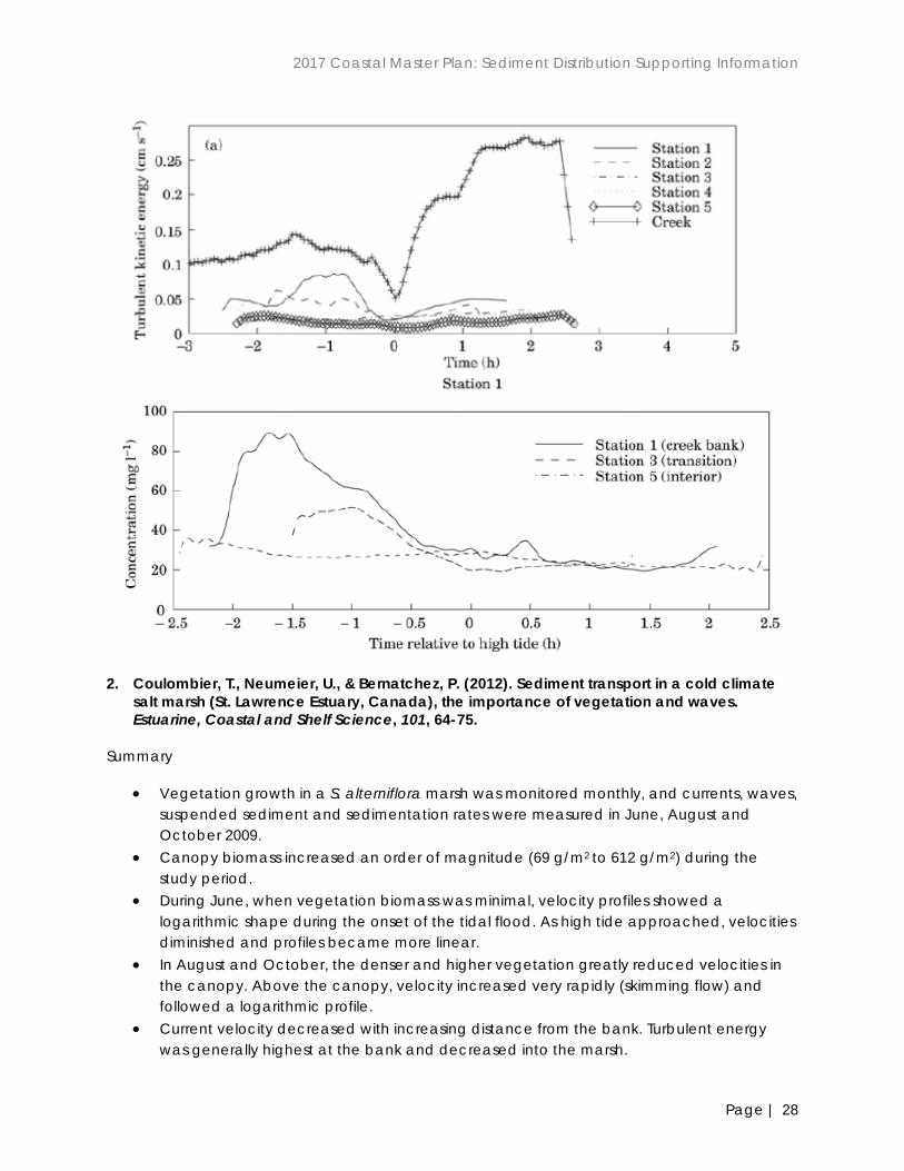
2. Coulombier, T., Neumeier, U., & Bernatchez, P. (2012). Sediment transport in a cold climate
salt marsh (St. Lawrence Estuary, Canada), the importance of vegetation and waves. Estuarine, Coastal and Shelf Science, 101, 64-75.
Summary
• Vegetation growth in a S. alterniflora marsh was monitored monthly, and currents, waves, suspended sediment and sedimentation rates were measured in June, August and October 2009.
• Canopy biomass increased an order of magnitude (69 g/m2 to 612 g/m2) during the study period.
• During June, when vegetation biomass was minimal, velocity profiles showed a logarithmic shape during the onset of the tidal flood. As high tide approached, velocities diminished and profiles became more linear.
• In August and October, the denser and higher vegetation greatly reduced velocities in the canopy. Above the canopy, velocity increased very rapidly (skimming flow) and followed a logarithmic profile.
• Current velocity decreased with increasing distance from the bank. Turbulent energy was generally highest at the bank and decreased into the marsh.

2017 Coastal Master Plan: Sediment Distribution Supporting Information
Page | 29
3. Graham, G. W., & Manning, A. J. (2007). Floc size and settling velocity within a Spartina anglica canopy. Continental Shelf Research, 27(8), 1060-1079.
Summary
• An experimental annular flume and floc imaging technology were used to produce a data set of the settling characteristics of particulates suspended within shallow vegetated flows.
• Turbid mud suspensions with concentrations of 100, 250 and 500 mg L-1 were injected through S. anglica (stem densities 200, 400 and 800 stems m-2) at current speeds of 0.1, 0.2 and 0.3 m s-1.
• Mean velocities exhibited inverse exponential relations with vegetation density. • TSS concentrations were 1-2 orders of magnitude lower than experienced in open-water
environments. • Floc settling velocities were inversely proportional to floc diameter.
4. Huang, Y. H., Saiers, J. E., Harvey, J. W., Noe, G. B., & Mylon, S. (2008). Advection, dispersion, and filtration of fine particles within emergent vegetation of the Florida Everglades. Water Resources Research, 44(4).
Summary
• Line source injections of 1 μm latex microspheres were made into 5 m long field flumes. • Advection, dispersion, and filtration of micrometer-sized particles varied between settings
that could be distinguished on the basis of flow regime and aquatic vegetation composition.
• This sensitivity of particle mobility to changes in flow and vegetation presents a challenge to scientists and engineers seeking to predict the transport of particles in wetland systems.
5. Lee, J. K., Roig, L. C., Jenter, H. L., & Visser, H. M. (2004). Drag coefficients for modeling flow through emergent vegetation in the Florida Everglades. Ecological Engineering, 22(4), 237-248.
Summary
• Vegetation parameters such as stem density and stem diameter were measured in the field, and related to flow velocities to obtain a functional form for the vegetation drag coefficient through linear regression of the logarithmic transforms of measured resistance force and Reynolds number.
• Field data in the Everglades marshes show that stem spacing and the Reynolds number are important parameters for the determination of vegetation drag coefficient.

2017 Coastal Master Plan: Sediment Distribution Supporting Information
Page | 30
6. Leonard, L. A., & Croft, A. L. (2006). The effect of standing biomass on flow velocity and
turbulence in Spartina alterniflora canopies. Estuarine, Coastal and Shelf Science, 69(3), 325-336.
Summary
• Flow velocity, turbulence intensity, and turbulent kinetic energy (TKE) are significantly reduced in vegetated marsh canopies and the reduction is inversely related to vegetation biomass present in the water column.
• Velocities and TKE were reduced roughly 50% within the first 5 m of overland flow (relative to levels in open-channel flow).
• These reductions in TKE have the potential to augment particle deposition and diminish TSS concentrations, and depositional fluxes likely increase as canopy density increases.
7. Leonard, L. A., Hine, A. C., & Luther, M. E. (1995). Surficial sediment transport and deposition processes in a Juncus roemerianus marsh, west-central Florida. Journal of Coastal Research, 322-336.
Summary
• Flow velocity, water level, TSS concentrations and sediment deposition were monitored in a Juncus marsh in Florida.
• Flow speeds were inversely related to distance from creek edge and also to stem density.

2017 Coastal Master Plan: Sediment Distribution Supporting Information
Page | 31
• TSS concentrations near the bank were reflective of those in the tidal creek source. However with increasing distance from the creek, current velocities decreased and a corresponding decrease in TSS concentration was observed.
• Rates of total deposition per tidal cycle, estimated with sediment traps, decreased from 24 g/m2/cycle at the bank to 9.5 g/m2/cycle 10 m into the marsh.
• Though winter storms tended to increase deposition rates, rates for both locations (bank and 10 m into the marsh) were higher during summer than winter.
8. Leonard, L. A., & Luther, M. E. (1995). Flow hydrodynamics in tidal marsh canopies. Limnology and Oceanography, 40(8), 1474-1484.
Summary
• High-frequency (5 Hz) in situ measurements of flow speed were collected in Spartina alterniflora, Juncus roemerianus, and Distichlis spicata canopies.
• Mean flow speed and turbulence intensity were inversely related to stem density and distance from creek edge.
• Flow energies decreased by roughly an order of magnitude when flows first encountered marsh vegetation, and continued to decrease with increasing vegetation density.
• Reductions in flow speed coupled with decaying energy provide the hydraulic mechanism for sediment deposition patterns commonly observed in marsh system.
9. Leonard, L. A., Wren, P. A., & Beavers, R. L. (2002). Flow dynamics and sedimentation in Spartina alterniflora and Phragmites australis marshes of the Chesapeake Bay. Wetlands, 22(2), 415-424.
Summary
• This study examined sediment deposition, sediment mobility and flow characteristics in Phragmites and S. alterniflora marshes to determine if variations in plant morphology affected flow properties and particle dispersion patterns.
• No differences were found between the marsh types with regard to mean velocities, turbulence reduction, TSS reduction, or deposition.
• In both marshes, maximum deposition occurred closer to open water, and the organic content of deposited sediments increased with distance into the marsh interior.
• These results suggest that differences in vegetation type do not significantly alter flow regime, sediment transport, or deposition patterns.
• However, other vegetation types with different morphological characteristics should be examined.
10. Moskalski, S. M., & Sommerfield, C. K. (2012). Suspended sediment deposition and trapping efficiency in a Delaware salt marsh. Geomorphology, 139, 195-204.
Summary
• Sediment deposition, TSS, particle size and trapping efficiency were measured along 5 parallel 100 m transects perpendicular to the stream bank in a vegetated marsh (S. patens/S. alterniflora mix; 640-1237 stems/m2).
2017 Coastal Master Plan: Sediment Distribution Supporting Information
Page | 32
• Suspended sediment concentration was highest at stations nearest the bank (1000 mg/L), and decreased 2 orders of magnitude (to 10 mg/L) within the first 10 m into the vegetated marsh.
• Deposition rates reflected the concentration patterns, with highest rates occurring near the bank (100g/m2/tidal cycle), diminishing to around 10 g/m2/tidal cycle at backmarsh sites.
• The in situ grain size distribution was much coarser than the disaggregated distribution, indicating the presence of floccules in the suspended sediment.
• Decreasing floc size from the levee to the back marsh, and a corresponding decrease in settling velocity, is necessary to explain observed sediment deposition patterns.
11. Mudd, S. M., D'Alpaos, A., & Morris, J. T. (2010). How does vegetation affect sedimentation on tidal marshes? Investigating particle capture and hydrodynamic controls on biologically mediated sedimentation. Journal of Geophysical Research: Earth Surface (2003–2012), 115(F3).
Summary
• Previously reported laboratory studies are combined with an 18-year record of salt marsh vegetation characteristics to quantify the relative importance of direct organic sedimentation, particle capture by plant stems, and enhanced settling due to turbulence reductions on vertical accretion in North Inlet, South Carolina.
• In dense vegetation (stem density > 10 m-1), and rapid flows (>0.4 m s-1), particle capture by plant stems accounted for greater than 70% of the sediment delivered to the marsh from tidally induced flood waters.
• Where velocities are slower (<0.1 m s-1), particle capture accounted for less than 10% of the delivery.
• Fertilization experiments resulted in increased biomass and ensuing turbulence reductions in the water column, and increased effective particle settling velocity and vertical accretion.
12. Neumeier, U. (2007). Velocity and turbulence variations at the edge of saltmarshes. Continental Shelf Research, 27(8), 1046-1059.
Summary
• Detailed profiles of velocity and turbulence were measured in a laboratory flume planted with Spartina angelica.
• A logarithmic velocity profile, present in the flume in front of the vegetation, was gradually altered to a skimming-flow profile, typical for submerged saltmarsh vegetation.
• The roughness length of the vegetation depended only on the vegetation canopy characteristics, and was not sensitive to current velocity or water depth.
• The reduced turbulence in the canopy and the high turbulence in the skimming flow above the canopy should both increase sediment deposition.
2017 Coastal Master Plan: Sediment Distribution Supporting Information
Page | 33
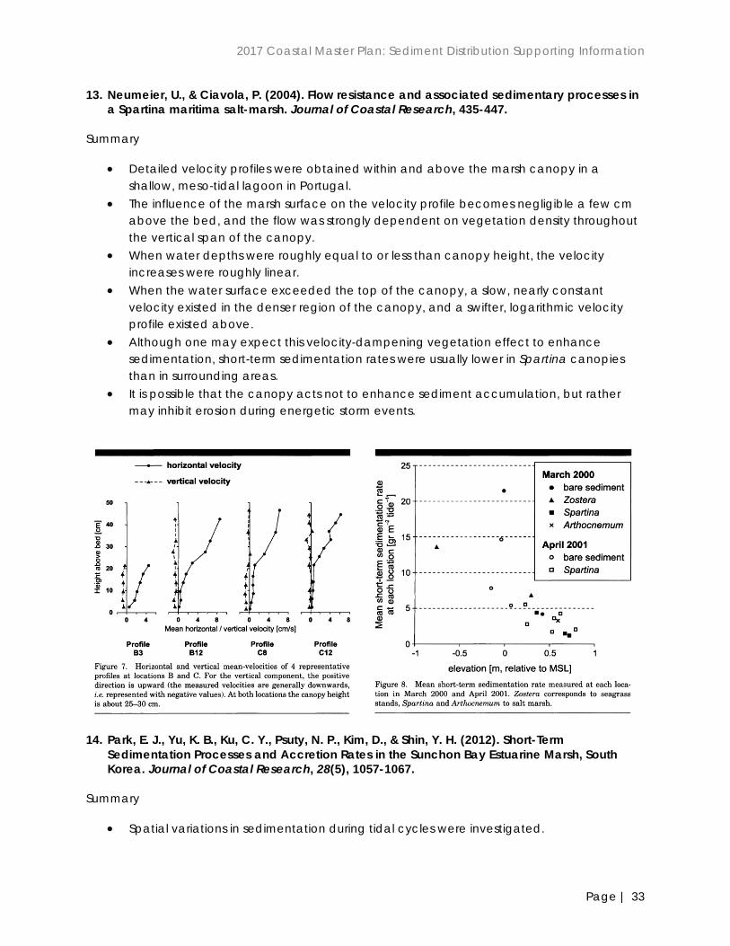
13. Neumeier, U., & Ciavola, P. (2004). Flow resistance and associated sedimentary processes in a Spartina maritima salt-marsh. Journal of Coastal Research, 435-447.
Summary
• Detailed velocity profiles were obtained within and above the marsh canopy in a shallow, meso-tidal lagoon in Portugal.
• The influence of the marsh surface on the velocity profile becomes negligible a few cm above the bed, and the flow was strongly dependent on vegetation density throughout the vertical span of the canopy.
• When water depths were roughly equal to or less than canopy height, the velocity increases were roughly linear.
• When the water surface exceeded the top of the canopy, a slow, nearly constant velocity existed in the denser region of the canopy, and a swifter, logarithmic velocity profile existed above.
• Although one may expect this velocity-dampening vegetation effect to enhance sedimentation, short-term sedimentation rates were usually lower in Spartina canopies than in surrounding areas.
• It is possible that the canopy acts not to enhance sediment accumulation, but rather may inhibit erosion during energetic storm events.
14. Park, E. J., Yu, K. B., Ku, C. Y., Psuty, N. P., Kim, D., & Shin, Y. H. (2012). Short-Term
Sedimentation Processes and Accretion Rates in the Sunchon Bay Estuarine Marsh, South Korea. Journal of Coastal Research, 28(5), 1057-1067.
Summary
• Spatial variations in sedimentation during tidal cycles were investigated.

2017 Coastal Master Plan: Sediment Distribution Supporting Information
Page | 34
• Deposition was higher at the creek bank than at the inner marsh, and decreased with distance from the estuary head.
• TSS concentrations in water exported from the marsh on the ebb tide were greatly reduced compared to those delivered on the flood.
• Accretion rates were strongly correlated with suspended loads.
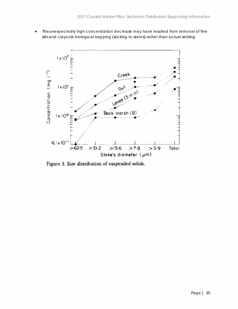
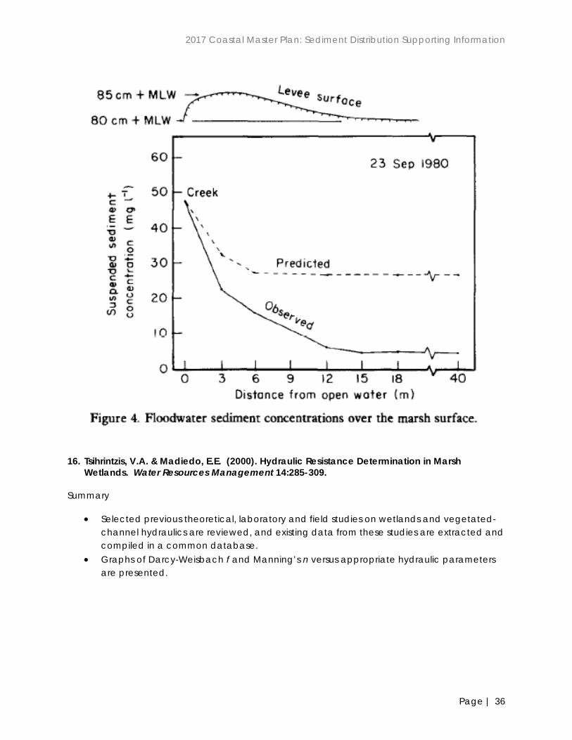
15. Stumpf, R.P. (1983). The process of sedimentation on the surface of a salt marsh. Estuarine,
Coastal and Shelf Science 17:495-508.
Summary
• This study investigates the movement of suspended sediment in tidal creek and marsh surface waters and compared settling rates of suspended sediment with the amount of deposited sediments.
• The quantity of suspended sediment reaching the back marsh during normal tides was inadequate to offset local sea level rise.
• Suspended sediments were much finer than deposited sediments, suggesting the water column was too energetic for deposition of fine particles.
• Normal tidal flooding did not appear to produce the bulk of sedimentation; rather, marsh elevations were maintained through very large depositional events associated with very severe storms that recur once each year.
• The decrease of concentration as a function of distance from flooding source decreased much more rapidly than was predicted by particle settling alone.
2017 Coastal Master Plan: Sediment Distribution Supporting Information
Page | 35
• This unexpectedly high concentration decrease may have resulted from removal of fine silts and clays via biological trapping (sticking to stems) rather than actual settling.
2017 Coastal Master Plan: Sediment Distribution Supporting Information
Page | 36
16. Tsihrintzis, V.A. & Madiedo, E.E. (2000). Hydraulic Resistance Determination in Marsh
Wetlands. Water Resources Management 14:285-309. Summary
• Selected previous theoretical, laboratory and field studies on wetlands and vegetated-channel hydraulics are reviewed, and existing data from these studies are extracted and compiled in a common database.
• Graphs of Darcy-Weisbach f and Manning’s n versus appropriate hydraulic parameters are presented.

2017 Coastal Master Plan: Sediment Distribution Supporting Information
Page | 37

2017 Coastal Master Plan: Sediment Distribution Supporting Information
Page | 38
17. Wang, H., Steyer, G.D., Piazza, S.C., Holm, G.O., Stagg, C.L., Rybczyk, J.M., Fischenich, C.J.,
Couvillion, B.C., Boustany, R.G., Fischer, M.R. & Sharp, L.A. (2012). Horizontal and vertical variability in soil bulk density and organic matter across coastal Louisiana wetlands detected by the Coastwide Reference Monitoring System (CRMS)-Wetlands. Presented at the 2012 State of the Coast Conference, New Orleans, LA.
Summary
• Profiles of organic matter and bulk densities in the upper 25 cm of marsh soils were collected 2006-2007.
• Bulk density increases with depth for active deltaic marsh, swamp, intermediate, and brackish marshes; BD decreases with depth for saline marshes.
• In contrast, organic matter decreases with depth for swamp, active deltaic marsh, intermediate and brackish sites and decreases with depth for saline marshes.

2017 Coastal Master Plan: Sediment Distribution Supporting Information
Page | 39
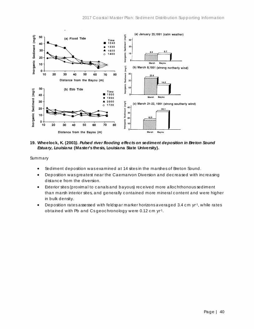
18. Wang, F.C., Lu, T. & Sikora, W.B. (1993). Intertidal marsh suspended sediment transport
processes, Terrebonne Bay, Louisiana, U.S.A. Journal of Coastal Research 9:209-220.
Summary
• Transport processes of suspended sediment from a tidal creek into its adjacent salt marsh were examined.
• Water samples were collected at multiple stations along a transect from the creek bank into the marsh.
• Sediment concentrations decreased from bayou bank to marsh interior during flood tides.
• During ebb tides, concentrations were reduced, and this spatial trend was absent. • Together these results indicate that sediment deposition occurred over the course of
tidal inundation events. Southerly winds, concentrations in the creek were much higher than those on the marsh; the opposite was true during northerly winds, suggesting that recently deposited sediments on the marsh may be re-suspended and exported.
• Estimates of bottom boundary shear stress during tidal inundations indicate that tidal events alone were insufficient to re-suspend sediments; storm events are more likely causes of erosion and export.
2017 Coastal Master Plan: Sediment Distribution Supporting Information
Page | 40
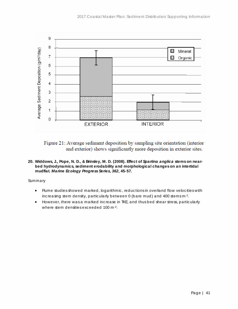
19. Wheelock, K. (2003). Pulsed river flooding effects on sediment deposition in Breton Sound
Estuary, Louisiana (Master’s thesis, Louisiana State University). Summary
• Sediment deposition was examined at 14 sites in the marshes of Breton Sound. • Deposition was greatest near the Caernarvon Diversion and decreased with increasing
distance from the diversion. • Exterior sites (proximal to canals and bayous) received more allochthonous sediment
than marsh interior sites, and generally contained more mineral content and were higher in bulk density.
• Deposition rates assessed with feldspar marker horizons averaged 3.4 cm yr-1, while rates obtained with Pb and Cs geochronology were 0.12 cm yr-1.
2017 Coastal Master Plan: Sediment Distribution Supporting Information
Page | 41
20. Widdows, J., Pope, N. D., & Brinsley, M. D. (2008). Effect of Spartina anglica stems on near-
bed hydrodynamics, sediment erodability and morphological changes on an intertidal mudflat. Marine Ecology Progress Series, 362, 45-57.
Summary
• Flume studies showed marked, logarithmic, reductions in overland flow velocities with increasing stem density, particularly between 0 (bare mud) and 400 stems m-2.
• However, there was a marked increase in TKE, and thus bed shear stress, particularly where stem densities exceeded 100 m-2:

2017 Coastal Master Plan: Sediment Distribution Supporting Information
Page | 42

2017 Coastal Master Plan: Sediment Distribution Supporting Information
Page | 43
• At the marsh edge under calm conditions, the near-bed flows were very low (<0.04 m s-1), with low bed shear stresses ((τ0<critical bed shear stress of 0.012 Pa). However, with intense wave activity, flow velocities doubled and bed shear stresses increased to 1.01 Pa, with τo>τcrit at velcoties > 0.03 m s-1:

2017 Coastal Master Plan: Sediment Distribution Supporting Information
Page | 44
• Morphological patterns existed at the marsh edge and subtidal mudflat that were consistent with these observations; a shallow depression was observed at the marsh edge and a raised shoulder of mud existed immediately seaward on the mudflat.
• Hydrodynamic data collected in the study suggest that most of the erosion occurred at the end of the ebb tide, with part of the resuspended sediment then being deposited in front of the salt marsh. This explanation is corroborated by the observations of higher TKE

2017 Coastal Master Plan: Sediment Distribution Supporting Information
Page | 45
in the marsh edge where the depression formed and greatly reduced TKE on the subtidal mudflat where the raised shoulder formed.
21. Yang, S.L., Li, H., Ysebaert, T., Bouma, T.J., Zhang, W.X., Wang, Y.Y., Li, P., Li, M. & Ding, P.X. (2008). Spatial and temporal variations in sediment grain size in tidal wetlands, Yangtze Delta: On the role of physical an abiotic controls. Estuarine, Coastal and Shelf Science 77:657-671.
Summary
• Measurements of surficial sediment grain size, canopy hydrodynamics, accretion and erosion rates, and vegetation characteristics were made in the Yangtze delta.
• High temporal variability in grain size was observed at a fixed site on an un-vegetated intertidal flat, which was attributed to seasonal and storm forcing.
• Coarser grain size distributions were found on the flat after storm events. • This temporal variability was greatly reduced in the vegetated, Spartina alterniflora marsh
site, owing to a combination of sediment adherence onto plants, and enhanced settling and reduced resuspension due to diminished turbulence.

2017 Coastal Master Plan: Sediment Distribution Supporting Information
Page | 46
4.0 Hurricane/storm-induced Sedimentation
1. Baumann, R.H., Day, J.W., Jr., & Miller, C.A. (1984). Mississippi deltaic wetland survival: sedimentation versus coastal submergence. Science, 224, 1093-1095.
Summary
• Study sites: 8 sites in Barataria Bay (BB) and 14 sites in Fourleague Bay (FB) (streamside and inland locations) between July 1975 and 1982.
• Method: feldspar marker horizon. • Source: reworked Barataria Bay bottom and marsh soils. • A hurricane (Hurricane Bob) and a tropical storm (TS Claudette) near Barataria Bay in
July 1979.

2017 Coastal Master Plan: Sediment Distribution Supporting Information
Page | 47
• Indicated that hurricane and tropical storm events in BB marsh deposited 36% of streamside and 40% of inland total sediment accumulation (less or no sediment from spring flooding). In contrast, the annual flood cycle during 1981 and 1982 contributed 91% and 69% of streamside and inland sediments to FB marshes.
• Found that hurricanes/storms resulted in wave-induced lateral erosion at 3 BB sites and one FB site and vertical erosion at 8 FB sites.
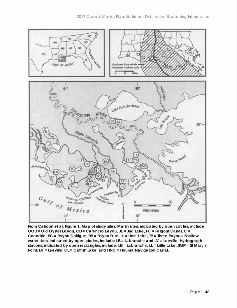
2. Cahoon, D. R., Reed, D. J., Day Jr, J. W., Steyer, G. D., Boumans, R. M., Lynch, J. C., & Latif, N. (1995). The influence of Hurricane Andrew on sediment distribution in Louisiana coastal marshes. Journal of Coastal Research, 280-294.
Summary
• Study area: salt marshes at Terrebonne, Barataria, and Pontchartrain basins. • Sampling sites: 11 (see their Figure 1). • Methods: sediment traps to calculate hurricane sediment deposition or accumulation
(g/m^2/d). • Sediment source: unconsolidated sediments within marsh channels and ponds. • Found that higher sediment deposition from Hurricane Andrew at sites closer to the storm
track (see their Figure 4). • Found indication of hurricane deposition was an increase in bulk density in the 2-3 cm soil
layer. • Indicated that interior marsh sites tended to have a lower BD than marsh sites near-shore
(Jug Lake site vs. Old Oyster Bayou, 0.15 vs. 0.8 g/cm^3), indicating different sources of hurricane sediments (sediments from lakes or ponds near marshes vs. offshore origin).
• Indicated that a storm can simultaneously influence both surface and subsurface soil processes with the net outcome on soil elevation not always predictable solely from the observed effects of sediment deposition and erosion. This influence on subsurface processes appears to be the single most important difference between high frequency, low magnitude and low frequency, high magnitude events.
2017 Coastal Master Plan: Sediment Distribution Supporting Information
Page | 48
From Cahoon et al. Figure 1: Map of study sites. Marsh sites, indicated by open circles, include: OOB = Old Oyster Bayou, CB = Carencro Bayou, JL = Jug Lake, FC = Falgout Canal, C = Cocodrie, BC = Bayou Chitigue, BB = Bayou Blue, LL = Little Lake, TB = Three Bayous. Shallow water sites, indicated by open circles, include: LB = Labranche and LV = Leeville. Hydrograph stations, indicated by open rectangles, include: LB = Labranche; LL = Little Lake; SMP = St Mary's Point; LV = Leeville; CL = Catfish Lake; and HNC = Houma Navigation Canal.
2017 Coastal Master Plan: Sediment Distribution Supporting Information
Page | 49
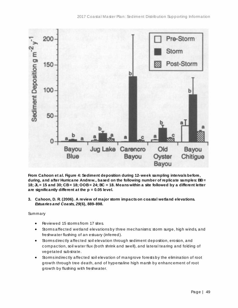
From Cahoon et al. Figure 4: Sediment deposition during 12-week sampling intervals before, during, and after Hurricane Andrew., based on the following number of replicate samples: BB = 18; JL = 15 and 30; CB = 18; OOB = 24; BC = 18. Means within a site followed by a different letter are significantly different at the p = 0.05 level. 3. Cahoon, D. R. (2006). A review of major storm impacts on coastal wetland elevations.
Estuaries and Coasts, 29(6), 889-898. Summary
• Reviewed 15 storms from 17 sites. • Storms affected wetland elevations by three mechanisms: storm surge, high winds, and
freshwater flushing of an estuary (inferred). • Storms directly affected soil elevation through sediment deposition, erosion, and
compaction, soil water flux (both shrink and swell), and lateral tearing and folding of vegetated substrate.
• Storms indirectly affected soil elevation of mangrove forests by the elimination of root growth through tree death, and of hypersaline high marsh by enhancement of root growth by flushing with freshwater.

2017 Coastal Master Plan: Sediment Distribution Supporting Information
Page | 50
• Storms can cause both sediment deposition and erosion in coastal wetlands (see his Table 1).
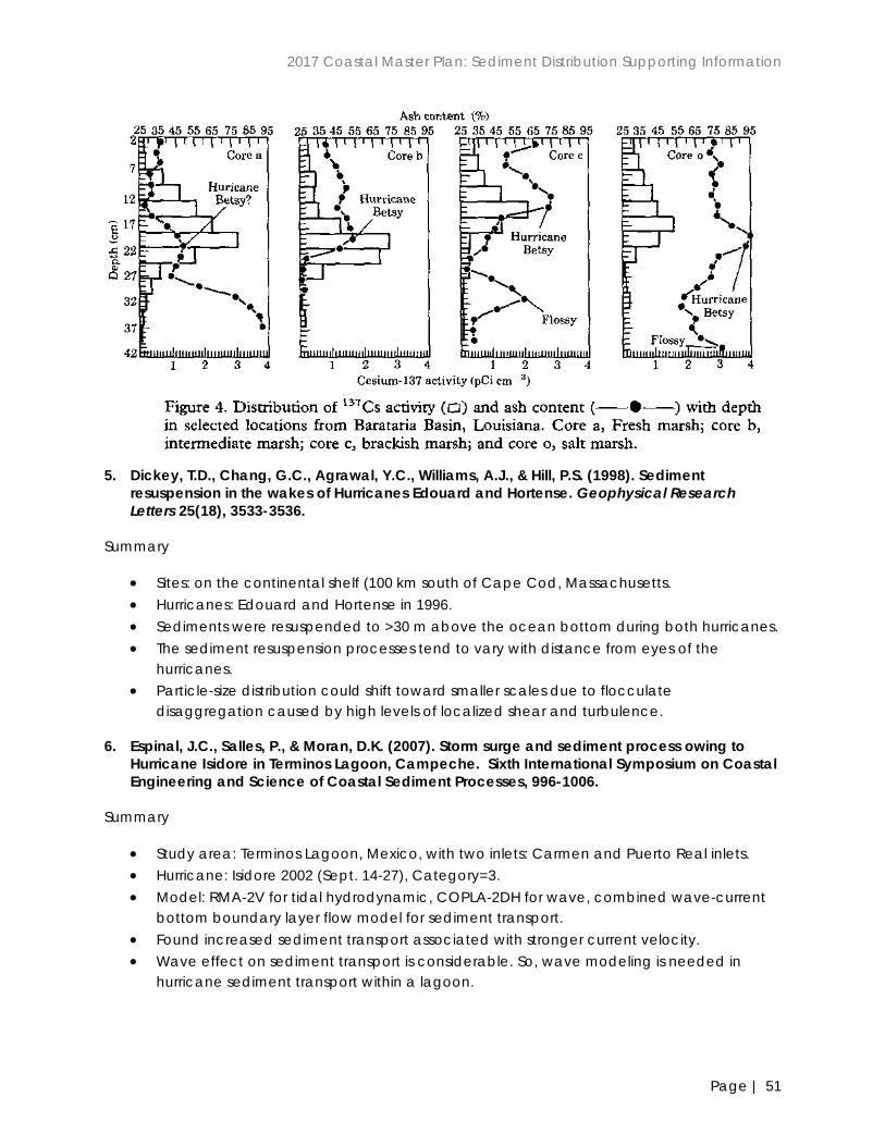
4. Chmura, G. L., & Kosters, E. C. (1994). Storm deposition and 137 Cs accumulation in fine-grained marsh sediments of the Mississippi Delta plain. Estuarine, Coastal and Shelf Science, 39(1), 33-44.
Summary
• Study sites: 15 sites from back marsh locations (>10 m from streamside) within fresh (6), intermediate (3), brackish (3) and salt (3) marshes of Barataria Basin during fall of 1985.
• Hurricanes: 20 of them during 1950-1985. • Method: 137Cs dating and ash (mineral matter) content analysis. • Indicated that impact of major hurricanes (e.g., Betsy 1969) on sediment accumulation
can be detected via identifying the coincidence of 137Cs activity peaks with mineral peaks.
• Indicated that location and occurrence of storm deposition is variable along a coast and can be localized within a bay since it is critically dependent on orientation of winds and tides.
• Found greatest impact on erosion and deposition would be by hurricane-force winds (>=74 mph), not by passage of winter fronts.
2017 Coastal Master Plan: Sediment Distribution Supporting Information
Page | 51
5. Dickey, T.D., Chang, G.C., Agrawal, Y.C., Williams, A.J., & Hill, P.S. (1998). Sediment
resuspension in the wakes of Hurricanes Edouard and Hortense. Geophysical Research Letters 25(18), 3533-3536.
Summary
• Sites: on the continental shelf (100 km south of Cape Cod, Massachusetts. • Hurricanes: Edouard and Hortense in 1996. • Sediments were resuspended to >30 m above the ocean bottom during both hurricanes. • The sediment resuspension processes tend to vary with distance from eyes of the
hurricanes. • Particle-size distribution could shift toward smaller scales due to flocculate
disaggregation caused by high levels of localized shear and turbulence.
6. Espinal, J.C., Salles, P., & Moran, D.K. (2007). Storm surge and sediment process owing to Hurricane Isidore in Terminos Lagoon, Campeche. Sixth International Symposium on Coastal Engineering and Science of Coastal Sediment Processes, 996-1006.
Summary
• Study area: Terminos Lagoon, Mexico, with two inlets: Carmen and Puerto Real inlets. • Hurricane: Isidore 2002 (Sept. 14-27), Category=3. • Model: RMA-2V for tidal hydrodynamic, COPLA-2DH for wave, combined wave-current
bottom boundary layer flow model for sediment transport. • Found increased sediment transport associated with stronger current velocity. • Wave effect on sediment transport is considerable. So, wave modeling is needed in
hurricane sediment transport within a lagoon.

2017 Coastal Master Plan: Sediment Distribution Supporting Information
Page | 52
7. Fagherazzi, S., Biberg, P.L., Temmerman, S., Struyf, E., Zhao, Y., & Raymond, P.A. (2013). Fluxes of water, sediments, and biogeochemical compounds in salt marshes. Ecological Processes 2: 3.
8. Fagherazzi, S., & Priestas, A.M. (2010). Sediments and water fluxes in a muddy coastline: interplay between waves and tidal channel hydrodynamics. Earth Surface Processes and Landforms 25, 284-293.
Summary
• Most sediment enters the marsh through tidal channels. • Suspended sediment in low marsh environments can be the product of wave-driven
resuspension in adjacent bays or tidally driven resuspension in tidal creeks. • The sediment input in a marsh is a function of SSC in water column and water discharge.
• SSC entering a marsh channel in muddy Louisiana coastline is proportional to the significant wave height in the bay.

2017 Coastal Master Plan: Sediment Distribution Supporting Information
Page | 53
• Storm surges represent ideal events for both sediment input and export in a marsh:
Sediment input processes: the strong wind associated with the storm produces waves that resuspend fine sediments in front of marshes, and the wind and wave setup increases the maximum tide level and thereby the water discharge during flood in the channels (by increasing the tidal prism; see their Equations 1, 2). Therefore during a storm surge both discharge and sediment concentrations of the entering water are magnified, augmenting the total volume of sediment imported in the marsh (Equation 4).
Sediment export processes: sediments are exiting the marsh through the channels during the subsequent ebb flow. The same physics governs the export of sediments, and Equation 4 is still valid but now the integral is evaluated from thigh to tlow.
o The sediment concentration of the exiting flow is now independent of the hydrodynamic conditions in the adjacent bays and tidal flats but is governed by physical processes mobilizing sediments within the salt marsh.
o Wind waves are negligible on marsh platforms, given the shallow water depths and the damping effect of vegetation (Möller et al. 1999). Therefore only tidal currents triggering high velocities are potentially responsible for sediment mobilization on the marsh surface during ebb, although field evidence seems to indicate that this effect is limited.
o Most of the sediment is therefore eroded and resuspended from the channels bottom and banks, where the velocities are high and vegetation does not protect the substrate. Data from Louisiana confirm that sediment concentration in the water exiting a marsh during ebb is proportional to the tidal velocity in the channel (see Figure below) (Fagherazzi and Priestas 2010). Moreover, given the low settling velocity of the fine material typical of marshlands, some of the sediment that was imported during flood might remain in suspension and exit the system during the following ebb.

2017 Coastal Master Plan: Sediment Distribution Supporting Information
Page | 54
o Storm surges, by increasing flow velocities, decrease the likelihood of particle
settling during high tide, reducing the potential accumulation of sediments on the marsh platform.
o Best conditions for sediment accumulation are moderate storms that increase sediment resuspension near salt marshes, but do not trigger fast flows in the channels (Fagherazzi and Priestas 2010).
o Proposed a simple model: The model can be obtained by considering an advection-dispersion equation governing the dynamics of suspended sediments over the marsh platform and by neglecting the advective and dispersive terms so that the variation in time of the concentration equals the settling rate.
o Wind-enhanced tidal and wave-generated bed shear stresses result in higher
concentrations of suspended sediment in the water flooding the marsh (Christiansen et al. 2000; Lawson et al. 2007; Fagherazzi & Priestas, 2010) and longer inundation times. As a result, deposition rates are higher and deposition extends further into the marsh during storm tides (e.g., Cahoon, 2006; Reed, 1989; Turner et al., 2006).
9. Gellis, A. (1993). The effects of hurricane hugo on suspended‐sediment loads, Lago loíza Basin, Puerto Rico. Earth Surface Processes and Landforms, 18(6), 505-517.
Summary
• Hurricane force winds seem to be the most important factor contributing to the lower than expected suspended sediment loads in the Lago Loiza basin.
• The high winds caused vegetation and debris to be dislodged and displaced. Debris accumulated on hill slopes and in small channels, blocked bridges and formed debris dams. These dams caused local backwater effects that reduced stream velocities and decreased suspended-sediment loads.

2017 Coastal Master Plan: Sediment Distribution Supporting Information
Page | 55
10. Goodbred, S. L., & Hine, A. C. (1995). Coastal storm deposition: salt-marsh response to a severe extratropical storm, March 1993, west-central Florida. Geology, 23(8), 679-682.
Summary
• Study area: Waccasassa Bay coastal ecosystem, FL. • Ten sampling sites. • Found absence of shoreline erosion along the marsh coast in contrast with sandy coast.
This might because the storm surge flooded the shore edge during storm and prevented wave cutting along the marsh shoreface.
• Found that along the shore edge, stabilization was enhanced through sediment binding by root mats of well-established Spartina alterniflora and Juncus roemerinus marsh plants. The thick Juncus canopy also inhibited surface erosion by baffling near-bed flow velocity. And erosion was further limited by the high critical shear stress of the cohesive, fine-grained marsh muds.
• Indicated that large-scale storm events may be an important component in sediment transport processes and marsh surface accumulation especially for coasts under sediment-poor, sand-starved and low energy conditions.
• Showed that hurricane sediment deposition thickness on marsh surface can reach several hundred meters from creek banks and shore edge, and decrease with distance into the marsh.
• Indicated that grain-size distribution varies in space: coarser near bay and finer with distance from water’s edge.
11. Guntenspergen, G. R., Cahoon, D. R., Grace, J., Steyer, G. D., Fournet, S., Townson, M. A., & Foote, A. L. (1995). Disturbance and recovery of the Louisiana coastal marsh landscape from the impacts of Hurricane Andrew. Journal of Coastal Research, 324-339.
Summary
• Study sites: 6 sites in western Terrebonne Basin. • Hurricane: Andrew 1992. • Hurricane impacted area classification: 1) compressed area, 2) thick sediment area, 3)
wrack area, 4) least impacted area, 5) scour area, and 6) salt burn area. • Source: sediment in the bottom of Atchafalaya Bay, by Atchafalaya River. At some sites
sediment was introduced from off shore areas while at other sites marsh sediments were redistributed.
• Found that the thickest sediments ranged from 9.8 to 16 cm and were deposited east of Atchafalaya and Four League Bays in the northeast quadrant of the track of the storm as it neared landfall. The sediments deposited by the storm averaged 10 x to 20 x greater than pre-storm deposition rates.
• Indicated that the input of this sediment onto coastal wetlands represents significant inputs relative to cold front passages and riverine inputs and represent another important source for their stability and survival.
• Found that Otter Bayou was far removed from off-shore sediment sources but the unstable and deteriorating marsh was eroded and re-deposited onto the remaining

2017 Coastal Master Plan: Sediment Distribution Supporting Information
Page | 56
marsh surfaces. Ripped, and eroded marsh was more prevalent in the Otter Bayou region because of the pre-storm condition of the marsh.
12. Horton, B. P., Rossi, V., & Hawkes, A. D. (2009). The sedimentary record of the 2005 hurricane season from the Mississippi and Alabama coastlines. Quaternary International, 195(1), 15-30.
Summary
• Three study sites: Ocean Springs, St. Andrews, MS, and Dauphine Island, AL.
o Ocean Springs, MS: 9.5 cm thick layer of medium to coarse grain sand was deposited by Hurricane Katrina.
o St. Andrews, MS: 9 and 7 cm thick by Katrina and Rita. o Dauphine Island, AL: 13 and 7 cm thick by Katrina and Rita.
• 2005 hurricane season from Mississippi and Alabama coastline: difference between the pre-storm surge and storm surge sediment: there is a sharp or erosional boundary between the two sedimentary units.
• The overlying storm surge sediment was coarser than the pre-storm surge sediment with a lower organic content. The boundary can be readily identified in the field and through grain size analysis.
13. Keen, T.R., & Glenn, S.M. (1997). Resuspension and advection of sediment during Hurricane Andrew on the Louisiana continental shelf. In Estuarine and Coastal Modeling pp. 481-494.
Summary
• Applied a coupled bottom boundary layer-sedimentation model for predicting sediment resuspension and transport on continental shelves.
• Revealed that sediment resuspension is mainly a result of wave action and operates at the time scale of wave period.
• Found that mass and elevation changes in the bed are associated with steady currents at long time scales (e.g., 1 hour) compared to storm wave periods (e.g., on the order of 10 seconds).
• Indicated that the strongest winds and highest waves were located east of the storm track.
14. Kirwan, M. L., & Murray, A. B. (2007). A coupled geomorphic and ecological model of tidal marsh evolution. Proceedings of the National Academy of Sciences, 104(15), 6118-6122.
Summary
• A spatial model for development of tidal marsh platform and channel network. • Spatial resolution: 5x5 m, time step = 0.5 day (one tidal cycle assumed semi-diurnal0.
Spatial extent: 3 km x 3 km. • The model can simulate volume of water that flows through a given cell (related to high-
tide level, and bed elevation); erosion rate (depending on bed shear stress); deposition rate (a function of vegetation biomass, SSC, and high-tide water depth.

2017 Coastal Master Plan: Sediment Distribution Supporting Information
Page | 57
• Slope-driven sediment transport is included.
15. Liu K., & Fearn, M.L., (2000). Holocene history of catastrophic hurricane landfalls along the Gulf of Mexico coast reconstructed from coastal lake and marsh sediments. In: Ning, Z., Abdollahi, K.K., (eds). Current Stresses and Potential Vulnerabilities: Implications of Global Change for the Gulf Coast Region of the United States. Franklin Press, Inc. and GCRCC.
Summary
• Study sites: Pearl River marsh, Atchafalaya marsh. • Hurricanes: Camille1969 (category 5, surge 6 m, a layer of clay) for Pearl River marsh,
Andrew 1992 (category 3, 5-16 cm thick sand or silt layer) for Atchafalaya salt marsh. • Methods: long cores (8.5 m at Pearl River marsh, 2.85 m and 7.9 m for Atchafalaya
marsh). • Indicated that the sedimentological and stratigraphic signatures of paleo-hurricanes can
be identified from coastal marshes in the form of distinct clastic (clay, silt, or sand, depending on sediment source) or inorganic layers embedded in peat deposits.
• Found that because of the topographic and hydrographic complexity of the marsh surface in relation to the source and direction of sediment supply during and after a storm surge event, this storm deposit may be uneven in thickness or spatially discontinuous.

2017 Coastal Master Plan: Sediment Distribution Supporting Information
Page | 58
16. McKee, K. L., & Cherry, J. A. (2009). Hurricane Katrina sediment slowed elevation loss in
subsiding brackish marshes of the Mississippi River delta. Wetlands, 29(1), 2-15. Summary
• Two sites at Pontchartrain Basin after Hurricane Katrina: Big Branch Marsh NWF and Pearl River Wildlife Management Area.
• Sediment source: Either organic soils in the interior marsh and nearby shallow pond areas, or offshore sediments.
• At Pearl River marsh: BD 1.36 g/cm3, mineral content 98%, TOC 0.5%, Sandy texture: sand 84%, silt 13%, clay 2%, significant differ from pre-storm layers. At Big Branch marsh: sand 31%, silt 36%, clay 5%, BD 0.2 g/cm3, OM32%, TOC 17.2%. Not significant from pre-storm layers.
• Found that the counterclockwise winds tend to bring more offshore sediment to Pearl River marsh on the east side and less sediment to Big Brach marsh on the west side of the Katrina track.
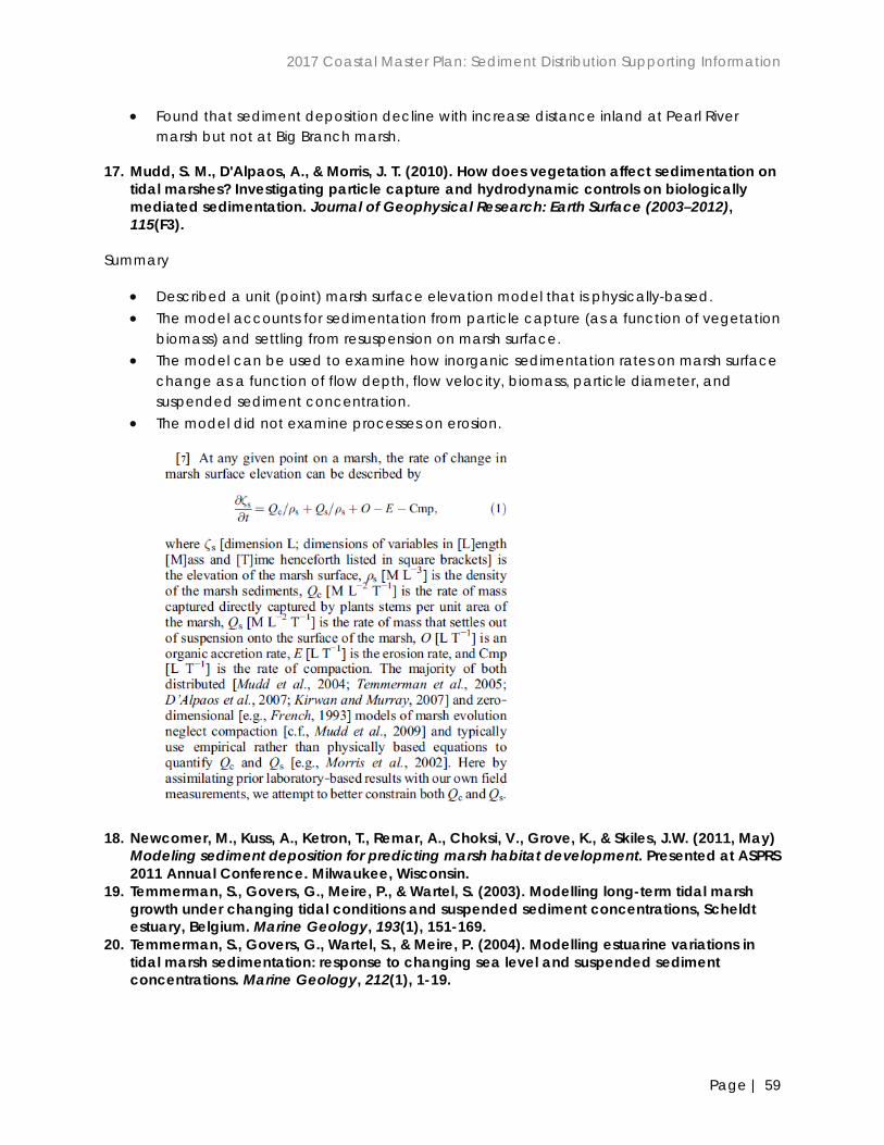
2017 Coastal Master Plan: Sediment Distribution Supporting Information
Page | 59
• Found that sediment deposition decline with increase distance inland at Pearl River marsh but not at Big Branch marsh.
17. Mudd, S. M., D'Alpaos, A., & Morris, J. T. (2010). How does vegetation affect sedimentation on tidal marshes? Investigating particle capture and hydrodynamic controls on biologically mediated sedimentation. Journal of Geophysical Research: Earth Surface (2003–2012), 115(F3).
Summary
• Described a unit (point) marsh surface elevation model that is physically-based. • The model accounts for sedimentation from particle capture (as a function of vegetation
biomass) and settling from resuspension on marsh surface. • The model can be used to examine how inorganic sedimentation rates on marsh surface
change as a function of flow depth, flow velocity, biomass, particle diameter, and suspended sediment concentration.
• The model did not examine processes on erosion.
18. Newcomer, M., Kuss, A., Ketron, T., Remar, A., Choksi, V., Grove, K., & Skiles, J.W. (2011, May) Modeling sediment deposition for predicting marsh habitat development. Presented at ASPRS 2011 Annual Conference. Milwaukee, Wisconsin.
19. Temmerman, S., Govers, G., Meire, P., & Wartel, S. (2003). Modelling long-term tidal marsh growth under changing tidal conditions and suspended sediment concentrations, Scheldt estuary, Belgium. Marine Geology, 193(1), 151-169.
20. Temmerman, S., Govers, G., Wartel, S., & Meire, P. (2004). Modelling estuarine variations in tidal marsh sedimentation: response to changing sea level and suspended sediment concentrations. Marine Geology, 212(1), 1-19.
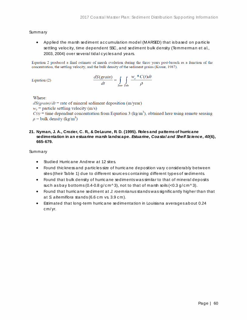
2017 Coastal Master Plan: Sediment Distribution Supporting Information
Page | 60
Summary
• Applied the marsh sediment accumulation model (MARSED) that is based on particle settling velocity, time dependent SSC, and sediment bulk density (Temmerman et al., 2003, 2004) over several tidal cycles and years.
21. Nyman, J. A., Crozier, C. R., & DeLaune, R. D. (1995). Roles and patterns of hurricane
sedimentation in an estuarine marsh landscape. Estuarine, Coastal and Shelf Science, 40(6), 665-679.
Summary
• Studied Hurricane Andrew at 12 sites. • Found thickness and particles size of hurricane deposition vary considerably between
sites (their Table 1) due to different sources containing different types of sediments. • Found that bulk density of hurricane sediments was similar to that of mineral deposits
such as bay bottoms (0.4-0.8 g/cm^3), not to that of marsh soils (<0.3 g/cm^3). • Found that hurricane sediment at J. roemrianus stands was significantly higher than that
at S. alterniflora stands (6.6 cm vs. 3.9 cm). • Estimated that long-term hurricane sedimentation in Louisiana averages about 0.24
cm/yr.

2017 Coastal Master Plan: Sediment Distribution Supporting Information
Page | 61

2017 Coastal Master Plan: Sediment Distribution Supporting Information
Page | 62
22. Parsons, M.L., (1998). Salt marsh sedimentary record of the landfall of Hurricane Andrew on
the Louisiana Coast: Diatoms and other paleoindicators. Journal of Coastal Research 14(3), 939-950.
23. Jackson, L. L., Foote, A. L., & Balistrieri, L. S. (1995). Hydrological, geomorphological, and chemical effects of hurricane Andrew on coastal marshes of Louisiana. Journal of Coastal Research, 306-323.
Summary
• Jackson et al. (1995): Hurricane Andrew caused erosion in intermediate/brackish marsh (losing 10-20 cm of sediment), resulting in converting to open water while a freshwater site was not affected. Therefore, effects of storm-induced sediment reworking within coast can results in sediment loss in some areas, but net sediment gain in others.
• Described hurricane sediment processes: As the storm approaches land, tides rise, and wind velocities and wave heights increase, leading to the development of a storm surge. A long-shore current generally develops moving from right to left (relative to the movement of the storm). Upon landfall, water currents move with direct influence from wind direction (counter-clockwise). Water and sediment are pumped out of the bays on the left side of the storm, and into bays on the right side. When the storm begins to wane, winds blow either offshore, or left to right, coupled with an offshore transport of sediment and water. Longshore currents reverse direction (left to right relative to the storm's path). After the storm has passed, mud settles out of suspension, and exposed fine-grained sediments are reworked.

2017 Coastal Master Plan: Sediment Distribution Supporting Information
Page | 63
• Indicated that Paleoindicators to distinguish hurricane sediment: 1) increased abundance of diatom species; 2) presence of marine species (also indicating a nearshore origin of the hurricane sediment); 3) elevated bulk density and decrease in OM indicating increased amounts of sand.
24. Reed, D. J. (1989). Patterns of sediment deposition in subsiding coastal salt marshes, Terrebonne Bay, Louisiana: the role of winter storms. Estuaries, 12(4), 222-227.
Summary
• Study sites: 2 sites (three filter papers at each site) near LUMCON, Terrebonne Bay. • Source for suspended sediment: not the two bayous, but the Terrebonne Bay. • Revealed that marsh sedimentation is not a continuous process (can only occur when
the marsh is flooded under flooding during high astronomical tide or under flooding during periods of strong winds and wave action (meteorological forcing) as well as passages of cold fronts.
• Found that southerly winds caused high waters, mobilizing sediments that are available for transport to marsh by flooding, northerly winds will reduce water level and suppress high tides, conditions that are not ideal for sediment transport onto marsh surface, but good for newly deposited sediment onto the marsh surface to drain and begin consolidation.
25. Rejmanek, M., Sasser, C. E., & Peterson, G. W. (1988). Hurricane-induced sediment deposition in a Gulf coast marsh. Estuarine, Coastal and Shelf Science, 27(2), 217-222.
Summary
• Study sites: near Willow Bayou (close to Atchafalaya Bay) in Terrebonne basin, representing four marsh communities, fresh, brackish or mixture of fresh and brackish marshes.
• Hurricanes: Danny on August 15-16, 1985; Juan Oct. 29-31, 1985. • Hurricane-induced sedimentation rate was measured by feldspar marker horizon
method. • Indicated that normal river flooding contributes little to marsh accretion rates in the area
compared to hurricane-induced sedimentation. • Indicated that there is a positive correlation between biomass and the amount of
hurricane-deposited sediments. • Showed the impact of hurricanes on sediment deposition at a small scale, the variability
in sedimentation is attributed to differences in plant community and local geomorphology.
• Found negligible sediment deposition after Hurricane Juan in their sites, but Chmura and Kosters (1994) observed ~7 cm of mud deposited locally at their site (also in BB) after Hurricane Juan.

2017 Coastal Master Plan: Sediment Distribution Supporting Information
Page | 64
26. Stumpf, R. P. (1983). The process of sedimentation on the surface of a salt marsh. Estuarine,
Coastal and Shelf Science, 17(5), 495-508. Summary
• Study area: Holland Glade Marsh (salt marsh) near Lewes, Delaware, with semi-diurnal tide, tidal range: 80 cm (tide-dominated marsh).
• Sampling from 5 neap and 8 spring tides between April 1980 and February 1981. • Hurricanes/storms: Oct. 25, 1980, a 25-year storm; on March 5-6, a small northeaster (not
hurricane). • During normal, storm-free conditions, tidal creek carries negligible amounts of sand and
coarse silt to marsh surface. Therefore, marsh has inadequate sedimentation for marsh vertical accretion to keep pace with SLR.
• Storms of a frequency of once per year can deposit sufficient sediment to maintain the marsh.
• The actual deposition of fine-grained sediment (fine silt and clay) appears to result primarily from biological trapping (veg and filter feeders) rather than from settling.
27. Teeter, A. M., Johnson, B. H., Berger, C., Stelling, G., Scheffner, N. W., Garcia, M. H., & Parchure, T. M. (2001). Hydrodynamic and sediment transport modeling with emphasis on shallow-water, vegetated areas (lakes, reservoirs, estuaries and lagoons). Hydrobiologia, 444(1-3), 1-23.
2017 Coastal Master Plan: Sediment Distribution Supporting Information
Page | 65
Summary
• A review paper on hydrodynamics, wind and wave, submersed plant friction, and sediment transport.
• Wind-generated waves (producing shear stresses) are important to sediment resuspension. In shallow water areas, waves ‘feel’ the bottom when wave length exceeds twice the depth, and the resulting bottom stress can resuspend sediments and dissipate the waves.
• Described three types of sediment transport models; governing equation is the advection-diffusion equation.
• Type-I: resuspension model; Type-II and III models: single- and multiple-grain-class model. • Erosion and deposition are simultaneously considered.
28. Temmerman, S., Bouma, T. J., Govers, G., Wang, Z. B., De Vries, M. B., & Herman, P. M. J. (2005). Impact of vegetation on flow routing and sedimentation patterns: Three‐dimensional modeling for a tidal marsh. Journal of Geophysical Research: Earth Surface (2003–2012), 110(F4).
Summary
• Used Delft3D model studying flow and sediment transport in a salt marsh in Scheldt estuary, SW Netherlands.
• Focused on the impacts of 1) vegetation, 2) micro-topography, and 3) water level fluctuations on spatial flow and sedimentation patterns in the tidal marsh landscape.
• Only considered the deposition of cohesive suspended sediment from the flooding water while bed erosion is ignored.
• Not considered tidal channel evolution or morphodynamics over longer time periods and from storms (need to include channel erosion).
• Resolutions: horizontal: 2 m x 2 m, vertical: 8 layers in sigma co-ordinate system; Time step = 3 seconds; the model was run for single tidal cycles.
• Data needed: Topography; Vegetation (stem diameter, density, height); boundary conditions (water level, and suspended sediment concentration (SSC).
29. Tweel, A.W., & Turner, R.E. (2012). Landscape-scale analysis of wetland sediment deposition from four tropical cyclone events. PlOS ONE 7(11), e50528.
Summary
• Generated maps of hurricane-induced sediment deposition from Hurricanes Katrina, Rita, Gustav, and Ike using the inverse distance weighting (IDW) on field sedimentation data (see their Figure 2).
• Indicated that storm-induced sediment depositions vary with distance from storm path and distance from coast (see their Figure 3): the majority of sedimentation (80%) occurred within the first 20 km inland, and declined exponentially. With distance from the storm track, about half (48%) of the total occurred within the first 50 km, but the distribution was more variable.

2017 Coastal Master Plan: Sediment Distribution Supporting Information
Page | 66
• Indicated that bulk density, mineral content, and grain size of hurricane sediment samples generally decrease inland, but vary substantially due to the impacts of finer scale factors (e.g., vegetation, local geomorphology).
• Discussed that the areas of high deposition generally coincided with the highest storm surges in previously reported models (Dietrich et al., 2011).

2017 Coastal Master Plan: Sediment Distribution Supporting Information
Page | 67
Tweel & Turner Figure 2. Wetland sediment deposition following four recent hurricanes. Mineral sediment deposition (g cm22) from Hurricanes Katrina (A), Rita (B), Gustav (C), and the Louisiana portion of Ike (D) interpolated using inverse distance weighting at 1 km2 resolution.

2017 Coastal Master Plan: Sediment Distribution Supporting Information
Page | 68
Tweel & Turner Figure 3. Distribution of mineral sediment with respect to distance from storm path and distance from coastline. 30. Turner, R. E., Baustian, J. J., Swenson, E. M., & Spicer, J. S. (2006). Wetland sedimentation from
hurricanes Katrina and Rita. Science, 314(5798), 449-452. Summary
• First study on coast wide (198 field sample sites) wetland sedimentation from hurricanes (Katrina and Rita).
• Reported coast wide hurricane sedimentation (thickness, accumulation, and bulk density) (see their Figure 2).
• Indicated that annualized average sediment accumulation from one hurricane could be 89% of the average accumulation in healthy salt marsh wetlands in the deltaic plain (0.166 g/cm^2/yr).

2017 Coastal Master Plan: Sediment Distribution Supporting Information
Page | 69
• Indicated that hurricane sediment deposition was greatest near the center of the storm track.
• Found that the deposits were generally thicker nearer landfall and also thicker on the margins of inlets such as Sabine Pass, probably because of reduced resistance to the passage of the storm surge (Williams, 2009).
31. Turner, R.E., Swenson, E.M., Milan, C.S., Lee, J.M. (2007). Hurricane signals in salt marsh
sediments: inorganic sources and soil volume. Limnology and Oceanography 52: 1231–1238. Summary

2017 Coastal Master Plan: Sediment Distribution Supporting Information
Page | 70
• Study sites (40 sites with 51 sediment cores) are located in salt marshes at St. Bernard Basin, Barataria Basin, and Terrebonne Basin.
• Linked inorganic density to 14 hurricanes between 1879 and 1990 (ranked as Category 3 storm and with a tidal surge >3 m).
• Found that peaks in bulk density were associated with each of these hurricanes. These peaks persist for 100 year, indicating that mixing is not sufficiently large to completely obliterate a signal arising from a storm of this size (Category 3).
• Indicated that the majority of sediments deposited on the marshes during hurricanes is from the Mississippi River.
32. Wang, F.C., Lu, T., & Sikora, W.B. (1993). Intertidal marsh suspended sediment transport processes, Terrebonne Bay, Louisiana, U.S.A. Journal of Coastal Research 9(1), 209-220.
Summary
• Tidal water movement and prevailing winds play a major role in the transport of suspended sediment in microtidal coastal Louisiana with negligible freshwater inflow.
• The transport processes of suspended sediment from a tidal creek/bayou onto its adjacent salt marsh during short-term periods over few tidal cycles, and processes of resuspension of cohesive sediment in coastal marshes in Louisiana are not fully understood.
• During flood tide, sediments were gradually deposited on marsh surface. • When northerly winds were strong (spring), sediment concentration in marsh surface
water were significantly much higher than that in the channel (tidal bayou/creek). • During the strong northerly winds, it is likely that some previously deposited sediments on
marsh surface can be resuspended and transported to bay by ebb-tide current. Indicating potential export of sediment from marsh (loss/erosion) during storm events. In contrast, strong southerly winds can mobilize sediment in the bay, then flood-tide current can transport sediment from the bay onto its adjacent marsh.
• Sediment deposited on the marsh surface were unlikely to be resuspended by tidal currents alone due to the smaller bottom shear stress (0.67 dyne/cm^2) than the value of critical shear stress (1 dyne/cm^2) for erosion (need strong winds, waves, e.g., from hurricanes).
• Suspended sediments in coastal bays can be transported both in and out of the bayou by tidal currents.
• Over-marsh surface flow (sheet flow) velocity increases with water depth on the marsh. • SSC were high near the mid-water level and were low at high-water level, implying
sediments are gradually deposited in marshes as the water floods over the marsh.
33. Williams, H. F. L., & Flanagan, W. M. (2009). Contribution of Hurricane Rita storm surge deposition to long-term sedimentation in Louisiana coastal woodlands and marshes. Journal of Coastal Research, 1671-1675.
Summary
• Study sites: woodland and marsh in Chenier Plain. • Hurricane: Rita 2005, data collected in Nov. 2005 and repeated in April 2007.

2017 Coastal Master Plan: Sediment Distribution Supporting Information
Page | 71
• Indicated that storm surge deposits are well-preserved in coastal woodland and marsh environments. Preserved storm sediment thickness ranged from 6.2 to 25 cm. These storm sedimentation data were compared with long-term sediment rates determined by 137Cs (0.24-0.71 cm/yr), indicating a single hurricane deposit may be the equivalent of over a century of non-storm-surge sedimentation.
• Issue: the long-term rates may include sedimentation from historical hurricanes/storms, not completely non-storm-surge sedimentation.
• The storm sedimentation at the two marsh sites (24.5 and 20 cm) may reflect the ability of the marshland surface to act as a sediment trap (due to wetter conditions, dense vegetation cover and generally lower elevations).
• Estimated that storm surge deposits may account for between one third and two thirds (27-66%) of long-term sedimentation based on the estimated recurrence interval of large hurricanes in the study area.
• Indicated that there are many factors that determine whether or not a hurricane generates a storm surge of sufficient height and energy to transport sediment into a particular site on the coast. These factors include distance from the eye of the storm, position in the left or right quadrant at landfall, magnitude of the hurricane, areal extent of the hurricane, forward speed of the storm, local tide levels, wave set up, wave run up, an available source of sediment, the height of topographic barriers to inundation and local topographic and/or bathymetric factors that either enhance or diminish storm surge height. Therefore, there is not a simple correlation between hurricane magnitude and storm surge sedimentation.
• Found that the beach and immediate offshore zone were the likely sources of washover sediments and no evidence was found of erosion and re-deposition of sediment from woodland and marsh surfaces.
34. Williams, H. F. (2012). Magnitude of Hurricane Ike storm surge sedimentation: implications for coastal marsh aggradation. Earth Surface Processes and Landforms, 37(8), 901-906.
Summary
• Hurricane Ike transported large amounts of offshore and littoral sediments into near-shore coastal marshes, forming a sandy to muddy sediment deposit extending hundreds to thousands of meters inland. So, the sources are beach and shallow offshore.
• Although riverine sediment inputs may be the ultimate source of sediment entering marshes in Chenier Plain, but reworked or remobilized by hurricanes.
• Hurricane sediments are readily distinguished from marsh sediments by their coarser texture, lower organic content and the presence of offshore foraminifera microfossils.
• Long-term impact of hurricane sedimentation depends not only on the magnitude of sediment input and retention, but also on the frequency of input into the marsh area.
• Observed marsh erosion around Sabine Pass with signs of shallow scouring caused by Hurricane Ike due to the explosion of the marsh edge to eave erosion during the storm surge.
• The thicknesses of hurricane sediment deposit generally decline with distance inland.

2017 Coastal Master Plan: Sediment Distribution Supporting Information
Page | 72
5.0 Utilization of Remote Sensors and Techniques to Quantify Suspended Sediment
Reflectance data from MODIS imagery has been used to track the plumes from the Bonnet Carré Spillway opening in 1997 (Haralampides 2000). Miller et al (2005) used MODIS reflectance to derive a resuspension potential for Lake Pontchartrain. Georgiou et al (2007) calibrated an ECOMSED model for Lake Pontchartrain using MODIS imagery. The circulation and the wave generated sediment processes were included in this ECOMSED model; the dominant forcing was found to be wind rather than tide. Since the open water areas of the Louisiana Coastal Area are generally shallow, the impact of wind wave induced resuspension is a major factor in the sediment distribution in open waters. 5.1 Landsat
1. Aranuvachapun, S., & Walling, D. E. (1988). Landsat-MSS radiance as a measure of suspended sediment in the Lower Yellow River (Hwang Ho). Remote Sensing of Environment, 25(2), 145-165.
This study in the Lower Yellow River, China used radiance measurements from the Landsat MSS satellite (60 m) to estimate suspended sediment concentrations in water. The authors used Munday and Alfoldi’s (1979) empirical algorithm calculated from their field experiment in the Bay of Fundy, Canada. Where R’ = radiance from the satellite and S = sediment data.
The previous author’s calculated a logarithmic relationship of u = 0.16 and v = 0.03 for band 5 of Landsat MSS. The above relationship was calculated in waters of a lower sediment concentration. Aranuvachapun, however, found it could be extended to also account for values in the hyperconcentration range of the Yellow River. The authors note that s sediment grain size plays a large part in reflectances seen in various water bodies and may account for differences between two different waters of similar sediment concentration but with varying spectral reflectances. The authors found this algorithm to be useful in estimating sediment concentrations and hope with further testing the algorithm could be proven universal. 2. Carpenter, D. J., & Carpenter, S. M. (1983). Modeling inland water quality using Landsat data.
Remote Sensing of Environment, 13(4), 345-352. Summary:
• Researchers completed multiple linear regression analysis between MSS reflectances and water quality parameters for multiple lakes in Australia which range from highly turbid to mostly clear some of which are prone to algal blooms.
• Turbidity (NTU) and algal pigment concentrations (chlorophyll a and pheopigments) were the water quality parameters identified.
• Landsat MSS was acquired for 7 dates in 1978 and 1979. • Relationships built between the two were limited to the date and data range of each
observation so data from multiple dates were pooled into one large dataset and sun

2017 Coastal Master Plan: Sediment Distribution Supporting Information
Page | 73
elevation was taken into account within the model in an attempt to compensate for differences in overall brightness between scenes.
• Predictive abilities of models were tested against separate datasets from this same lake and two other outside lakes.
• Sampling models fitted the data well with R2 values ranging from 0.59-0.95 for turbidity. • The best performing model was:
(B4= band 4, B5= band 5, B6= band 6, and SUN = sine of the sun elevation at the time of satellite overpass).
• Results suggest MSS satellite data can be a useful tool in monitoring water quality after completing relatively limited ground-based data.
3. Dekker, A. G., Vos, R. J., & Peters, S. W. M. (2002). Analytical algorithms for lake water TSM estimation for retrospective analyses of TM and SPOT sensor data. International Journal of Remote Sensing, 23(1), 15-35.
Summary
• Dekker’s method allows for a retrospective modeling of remote sensing data to compare to suspended matter concentrations independent of in situ measurements.
• Analytical optical modeling (bio-optical model) is instead used to study the backscattering and reflectance properties of the waters in question. These lead to reliable multi-temporal algorithms for estimating suspended matter concentrations in lakes from Landsat TM sensors.
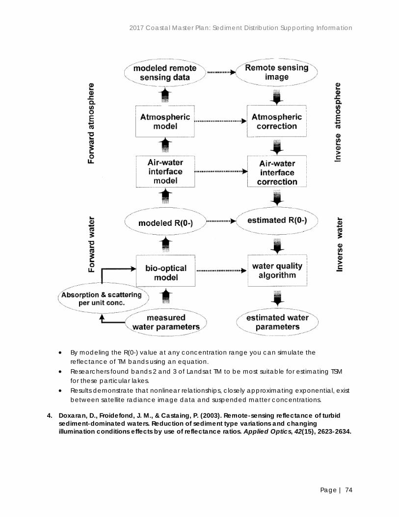
2017 Coastal Master Plan: Sediment Distribution Supporting Information
Page | 74
• By modeling the R(0-) value at any concentration range you can simulate the reflectance of TM bands using an equation.
• Researchers found bands 2 and 3 of Landsat TM to be most suitable for estimating TSM for these particular lakes.
• Results demonstrate that nonlinear relationships, closely approximating exponential, exist between satellite radiance image data and suspended matter concentrations.
4. Doxaran, D., Froidefond, J. M., & Castaing, P. (2003). Remote-sensing reflectance of turbid sediment-dominated waters. Reduction of sediment type variations and changing illumination conditions effects by use of reflectance ratios. Applied Optics, 42(15), 2623-2634.

2017 Coastal Master Plan: Sediment Distribution Supporting Information
Page | 75
Summary
• The aim of this study is to develop such an efficient and invariant inversion algorithm in estuarine sediment-dominated waters, which could permit the accurate estimation of the suspended particulate matter (SPM) distributions from satellite remotely sensed data, without carrying out field measurements for validation at the moment of the image acquisition.
• Mean SPM concentrations vary from 150 to approximately 3000 mg/l in surface waters of the estuary.
• The physical parameter usually considered in ocean color analyses is the irradiance reflectance, R(0-) defined as the ratio of the upwelling to downwelling irradiances just beneath the surface, R(0-) can be written as a function of the inherent optical properties (IOPs) of the water body, namely, the absorption and backscattering coefficients.
• The satellite reflectance signal can be retrieved from satellite measurements corrected for atmospheric effects. Reflectance can be related to the IOPs if the geometrical parameters that take into account the air–water interface transfer and bidirectional aspects are considered.
• The obtained R signals are then converted into SPM concentrations, according to an empirical relationship adapted to the study area. This empirical relationship is established from numerous in situ spectroradiometric measurements (400–1100 nm) carried out simultaneously with SPM concentration measurements within the surface water 0–1 m depth. Spectroradiometric data are weighted by sensitivity to obtain the equivalent R signal in spectral band of satellite sensors (Landsat).
• Finally, empirical relationships are established between the R signal and SPM, and the best ones are selected to quantify the SPM concentrations. Numerous in situ measurements are needed to improve the validity of the obtained relationship and to determine its limits.
• Optical properties of sediments (absorption and backscattering coefficients) are approximately proportional to the sediment concentration. Consequently, results demonstrated that empirical relationships between R in the near infrared and SPM concentration can be established. However, variations of particles’ grain size and refractive index modify their optical properties, and, consequently, the established empirical relationships. The variations of the particles’ grain size occur in estuaries during the tidal cycle.
• As the obtained relationships include all measurements carried out in the estuary from 1996 to 2001, they can be used to quantify the SPM from SPOT and Landsat satellite data independently of their date of acquisition, at least during this 6-yr period.
5. Fraser, R. N. (1998). Multispectral remote sensing of turbidity among Nebraska Sand Hills lakes. International Journal of Remote Sensing, 19(15), 3011-3016.
Summary
• Researchers studied correlations between field measured turbidity and multispectral reflectance data from Landsat TM in 21 different Nebraska lakes.
• Turbidity ranged from 2.7-82.3 NTU.

2017 Coastal Master Plan: Sediment Distribution Supporting Information
Page | 76
• Linear models yielded significant correlations between TM reflectances and turbidity field data which was collected in situ (while satellite was overpassing).
• Landsat TM bands 1 and 3 were strongly related with turbidity values after linear regression.
6. Hadjimitsis, D. G., Hadjimitsis, M. G., Clayton, C., & Clarke, B. A. (2006). Determination of turbidity in Kourris Dam in Cyprus utilizing Landsat TM remotely sensed data. Water Resources Management, 20(3), 449-465.
Summary
• Landsat 5- TM and Landsat-7 (ETM+) were compared for use in measuring turbidity within a dam in Cyprus.
• Linear regression analysis was used to compare these satellite reflectances to field derived turbidity values.
• Study lead to two regression predictive equations for determining turbidity (p = reflectance):
7. Harrington, J. A., Schiebe, F. R., & Nix, J. F. (1992). Remote sensing of Lake Chicot, Arkansas:
monitoring suspended sediments, turbidity, and secchi depth with Landsat MSS data. Remote Sensing of Environment, 39(1), 15-27.
Summary
• Landsat MSS satellite data was used in an Arkansas lake to monitor suspended sediment concentrations, turbidity, and secchi depth.
• Different models were tested ranging from simple linear regressions, simple linear regressions using log transformations, and optimized curve fitting.
• Researchers found that Landsat MSS band 3 provided the greatest ability to monitor the range of suspended sediment levels that are of most concern in lake resource management (0-500 mg/L).
• Researchers also found that Landsat MSS band 3 was most useful in estimating turbidity. • Turbidity resulted in the highest coefficients of determination and optimized curve fitting
was the best model.
8. Islam, M. R., Yamaguchi, Y., & Ogawa, K. (2001). Suspended sediment in the Ganges and Brahmaputra Rivers in Bangladesh: observation from TM and AVHRR data. Hydrological Processes, 15(3), 493-509.
Summary
• Suspended sediment in the Ganges and Brahmaputra Rivers in Bangladesh was studied using Landsat TM (band 3) for two discharge periods (both high and low).
• SSCs in these rivers are very high (1000-1300 mg/L).
2017 Coastal Master Plan: Sediment Distribution Supporting Information
Page | 77
• Reflectances were concerted to SSC by using a regression model. • It was observed that distribution patterns of reflectance matches well with the distribution
of SSC along the rivers. • The regression model used for estimating SSC was affected by the lack of sufficient in situ
data.
9. Keiner, L. E., & Yan, X. H. (1998). A neural network model for estimating sea surface chlorophyll and sediments from thematic mapper imagery. Remote sensing of environment, 66(2), 153-165.
Summary
• A neural network was used to model the relationship between sediment concentrations and satellite radiances from the Landsat TM for the Delaware Bay.
• A neural network with two hidden nodes using three visible Landsat TM bands were able to model the relationship better than a traditional regression analysis.
• In coastal waters, sediments and dissolved organic matter strongly affect water body’s spectral characteristics. Because of this in situ data must be collected at the time of satellite overpass and sometimes this must be done for separate seasons to account for variations. Surface chlorophyll-a, suspended sediment concentrations were measured throughout the bay. Suspended sediment concentrations ranged from 3.55-27.78 mg/L.
• Regression analysis is the typical method for modeling relationships between a field measured water quality and satellite reflectances. Various combinations of bands or band ratios are used to model these relationships. The best combination for sediment was the log-linear equation using only band 3.
• Neural networks have the ability to model nonlinear behavior. These models are trained and use weights, and biases in order to best model the data.
• Neural networks outperformed regression analysis. • The researchers recommend that future studies include more in situ samples for training
of the neural network which should include multi-date analysis. At least 30 samples should be obtained with a wide range of values. Neural networks are excellent interpolators but not great at extrapolating in ranges outside the training set.
10. Lathrop, R. G., Lillesand, T. M., & Yandell, B. S. (1991). Testing the utility of simple multi-date Thematic Mapper calibration algorithms for monitoring turbid inland waters. Remote Sensing, 12(10), 2045-2063.
Summary
• In situ water quality data (including surface measurements of total suspended solids, secchi disk depth, chlorophyll-a, turbidity, absorbance, and temperature) were collected in Green Bay, Lake Michigan.
• Linear regression analysis was used to quantify the relationship between field measured water quality data (SDD and TSS) and Landsat TM reflectances. An exponential model was found to typify the data best. It accounted for most of the nonlinearity in the satellite/ground data relationship.
• Band ratios generally improved accuracies of fit. (Band 3/Band 1) worked the best.
2017 Coastal Master Plan: Sediment Distribution Supporting Information
Page | 78
11. Mertes, L. A., Smith, M. O., & Adams, J. B. (1993). Estimating suspended sediment concentrations in surface waters of the Amazon River wetlands from Landsat images. Remote Sensing of Environment, 43(3), 281-301.
Summary
• Landsat TM and MSS data were used to determine suspended sediment in Amazon River waters.
• Reference spectra were measured in the laboratory using various water-sediment mixtures with a range of suspended sediment concentrations.
• The wavelengths of 400nm to 1000nm are most useful in determining sediment concentration values from satellite reflectances due to the low rates of absorption by the water and high rates of scattering.
• A linear mixture analysis was used to estimate sediment concentrations based on a nonlinear calibration curve between lab sediment concentrations and lab reflectances.
• Spectral mixture analysis has been used in the past to analyze vegetation, soils at subpixel scales. Here it was used to estimate sediment concentrations from Landsat images and lab derived spectra.
• Results are believed to be within +/- 20 mg/L.
12. Ritchie, J.C., & Cooper, C.M. (1991). An algorithm for estimating surface suspended sediment concentrations with Landsat MSS digital data. Water Resources Bulletin, 27:3, 373-379.
Summary
• Landsat MSS data was used in conjunction with in situ surface suspended sediment measurements to study a reservoir in Mississippi.
• Field measurements found suspended sediment concentrations ranging from 2 to 168 mg/L.
• Linear and polynomial regression techniques were used to better understand the relationship between suspended sediment concentrations and Landsat reflectances.
• It was found that Landsat MSS band 2 and 3 were most useful. • The equation below provided the best fit to the data and is very similar to the algorithm
used by Topliss et al (1990) for estimating surface suspended sediment concentrations.
• Studies in two other lakes found band 3 of Landsat MSS to be most useful in determining relationships between reflectances and suspended sediment concentrations. The authors believe this may be due to their higher surface suspended sediment concentrations (average of 110-183 mg/L). Band 2 is better in lakes with lower suspended sediment concentrations.
• In this study band ratios did not provide a better single equation.

2017 Coastal Master Plan: Sediment Distribution Supporting Information
Page | 79
13. Rouse, L. J., & Coleman, J. M. (1976). Circulation observations in the Louisiana Bight using LANDSAT imagery. Remote Sensing of Environment, 5, 55-66.
Summary
• Turbidity contours were estimated for waters around the Mississippi River Delta (sediment plume) using Landsat MSS satellite imagery and laboratory measured radiometer reflectances.
• Laboratory measured reflectances were calculated for concentrations ranging from 0 to 1500 mg/L.
• Radiance values from the satellite data were associated with suspended sediment loads and resulting data was contoured to give a map distribution of suspended sediment loads.
14. Song, K., Wang, Z., Blackwell, J., Zhang, B., Li, F., Zhang, Y., & Jiang, G. (2011). Water quality monitoring using Landsat Themate Mapper data with empirical algorithms in Chagan Lake, China. Journal of Applied Remote Sensing, 5(1), 053506-053506.
Summary
• Landsat thematic mapper (TM) data and in situ water samples collected concurrently with satellite overpass were used for the analysis, in which four important water quality parameters are considered: chlorophyll-a, turbidity, total dissolved organic matter, and total phosphorus in surface water.
• Empirical regressions and neural networks were established to analyze the relationship between the concentrations of these four water parameters and the satellite radiance signals. Neural network model out performed empirical regressions with TM visible and near-infrared bands as spectral variables.
• A bulk of studies indicated that Landsat-TM band 2 (525 to 605 nm) can be used to measure phytoplankton concentrations; band 3 (630 to 690 nm) can provide valuable information when large sediment loads occur and pigment as well; and band 4 (750 to 900 nm) is the spectral region where strong water absorption occurs, but the band reflectance is dominated by suspended matter.
• Investigations also demonstrated that band ratios or band combinations are more valuable for water quality monitoring because atmospheric effects and illumination variation can be reduced somehow in band ratios process.
• There are two main methods to estimate surface water quality parameters. One is the use of empirical algorithms derived from remotely sensed reflectance data. They can provide site specific predictions of water quality parameters with reasonable accuracy, but with no universal application.
• The other approach is the use of analytic inversion models that require the solution of radiative transfer equations for deriving absorption and scattering coefficients. The latter approach allows remote sensing measurements to be understood in terms of the inherent optical properties, and provides insight into the characteristics of the differences in algorithm coefficients for various regions.

2017 Coastal Master Plan: Sediment Distribution Supporting Information
Page | 80
5.2 Neural Network
• A neural network can model a large number of nonlinear behaviors without prior knowledge on the nature of nonlinearity and has the advantage over the standard linear regression with which nonlinearity cannot be modeled properly.
• It is preferred over a nonlinear regression because the latter requires a priori knowledge of the nature of the nonlinear behavior. A neural network is often suitable for situations where nonlinearity or chaotic is in datasets to be analyzed, or when the signal is deeply hidden within noise or other signals.
• For this study, a three layer neural network algorithm was used: an input layer, a hidden layer, and an output layer. The first layer distributes the input parameters of extracted data at different TM bands or band combinations to the second layer. The second layer (hidden layer) has a varying number of neurons, where each input parameter is multiplied by its connection’s weights and all the inputs to the neurons are summed and passed through a nonlinear sigmoid function (we choose tansig in this study). The third layer receives the output of the second layer in which it is processed through neurons again.
• The neural network method should be expanded to evaluate multidate imagery data for operational applications.
• Increased training samples will help the neural network perform better. Samples covering the entire range of water parameters in the study area should be obtained for the training purpose.
• Phytoplankton species and different suspended sediment types could be present in the water through different seasons and affect reflectances. These variations in phytoplankton species, inducing the variation in water spectral signatures, may change the inversion model parameters; even in some of the sensitive spectral bands.
15. Sudheer, K. P., Chaubey, I., & Garg, V. (2006). Lake water quality assessment from Landsat thematic mapper data using neural network: an approach to optimal band combination selection. Journal of the American Water Resources Association, 42(6), 1683-1695.
Summary
• This study aimed to better understand which satellite bands should be used in artificial neural network (ANN) studies of water quality (sediment concentration) in an Arkansas reservoir.
• Generally in most ANN studies of water quality, researchers develop their inputs either through time consuming trial and error or arbitrary decisions.
• These researchers note that an overabundance of input data causes an ANN model to significantly increase the learning complexity and hence lead to a reduced performance of the model.
• It was found that an ANN model that included Bands 1, 2, 3, and 4 outperformed all other band combinations tested.
2017 Coastal Master Plan: Sediment Distribution Supporting Information
Page | 81
16. Topliss, B. J., Almos, C. L., & Hill, P. R. (1990). Algorithms for remote sensing of high concentration, inorganic suspended sediment. International Journal of Remote Sensing, 11(6), 947-966.
Summary
• If algorithms change with their location and season then their utility is reduced, and extensive ground truth studies are inevitable.
• In situ suspended sediment data are not available for this papers study are of the Bay of Fundy. Instead, aircraft reflectance data from a previous study were used to estimate sediment reflectances and create an algorithm that will predict suspended sediment concentrations.
• Ratio and logarithmic algorithms gave the best results but ultimately equations with a pair of ratios gave the best results. Band 4/5 ratios were used for concentrations of 5-100 mg/L and band 5/6 were used for concentrations of between 100 to 1000 mg/L.
• Errors were found to be between 5-100 mg/L. Concentrations were under-estimated at very high concentrations.
17. Volpe, V., Silvestri, S., & Marani, M. (2011). Remote sensing retrieval of suspended sediment concentration in shallow waters. Remote Sensing of Environment, 115(1), 44-54.
Summary
• This paper aimed to estimate suspended sediment concentrations in the Venice lagoon using turbidity field data and multiple satellite sensors including Landsat TM. Shallow waters make estimation of suspended sediment particularly difficult because of bottom sediment signatures.
• This study used a radiative transfer model (like the above Dekker, 2002) to relate satellite reflectances and in situ turbidity observations.
• A bootstrap and cross-validation procedure was used to analyze the data. • A new suspended sediment concentration retrieval algorithm was developed based on
the radiative transfer model. • Several multispectral sensors were tested (including Landsat) and results between all of
them were consistent.
5.3 MODIS, AVHRR, SeaWifs and Other Coarse Spatial, High Temporal Resolution Sensors
1. Chen, Z., Hu, C., & Muller-Karger, F. (2007). Monitoring turbidity in Tampa Bay using MODIS/Aqua 250-m imagery. Remote Sensing of Environment, 109(2), 207–220. http://dx.doi.org/10.1016/j.rse.2006.12.019.
Summary
• Approach to map turbidity in estuaries using a time series. • 250 m resolution images from the Moderate Resolution Imaging Spectroradiometer
(MODIS) were used.

2017 Coastal Master Plan: Sediment Distribution Supporting Information
Page | 82
• Field data consisted of Turbidity data collected by the Tampa Bay water quality monitoring program which conducts monthly surveys that span 3 weeks with each week covering approximately one segment of the Bay.
• Noted that the relationship between turbidity and sediment concentration varies depending on sediment properties, and as such, field data was needed for calibration.
• In situ hyperspectral data were integrated over the relative spectral response (RSR) function of MODIS band 1 to obtain Rrs(645) for MODIS validations.
• MODIS Rrs(645) ranging from 0.001 to 0.008 sr−1 is closely correlated with in situ turbidity values from 0.9 to 8.0 NTU (turbidity=1203.9×Rrs(645)1.087, r2 =0.73, n=43).
• More importantly, this relationship appeared to be stable over 2004 and 2005, indicating that the regression is time independent.
• Noted likely artifacts due to the interference by CDOM. “Therefore, high CDOM absorption will reduce Rrs(645) and yield low, unrealistic turbidity retrievals."
• Concluded that "repeated, frequent, and synoptic coverage of estuarine regions provided by MODIS satellite data across the globe, and because these data are robust, low cost, and simple to use, satellite data from sensors such MODIS are important complements of traditional in situ water quality surveys".
2. Doxaran, D., Froidefond, J. -M., Castaing, P., & Babin, M. (2009). Dynamics of the turbidity maximum zone in a macrotidal estuary (the Gironde, France): Observations from field and MODIS satellite data. Estuarine, Coastal and Shelf Science, 81(3), 321–332. http://dx.doi.org/10.1016/j.ecss.2008.11.013.

2017 Coastal Master Plan: Sediment Distribution Supporting Information
Page | 83
Summary
• Over a 1-year period, field and satellite measurements of surface water turbidity were combined in order to study the dynamics of the turbidity maximum zone (TM) in a macrotidal estuary (the Gironde, France).
• Field data were used to validate a recently developed SPM quantification algorithm applied to the MODIS ‘surface reflectance’ product.
• SPM was estimated by:
• Field measurements were used to establish the relationship between the SPM concentration in the Gironde estuary and the MODIS B2 to B1 water reflectance ratio (R21 ¼ R(B2)/R(B1)):
• The relative uncertainty of the algorithm applied to these sensors was found to vary
between 22% and 18%.
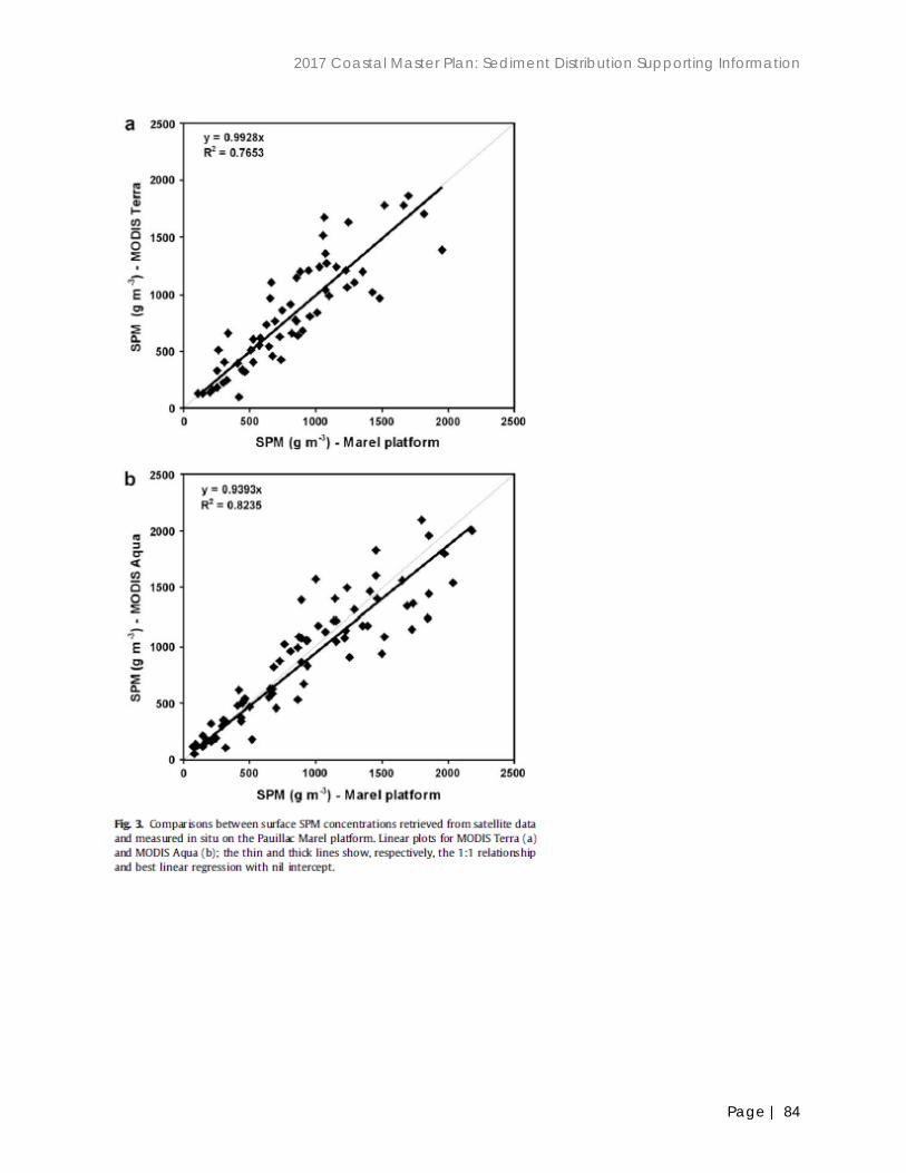
2017 Coastal Master Plan: Sediment Distribution Supporting Information
Page | 84
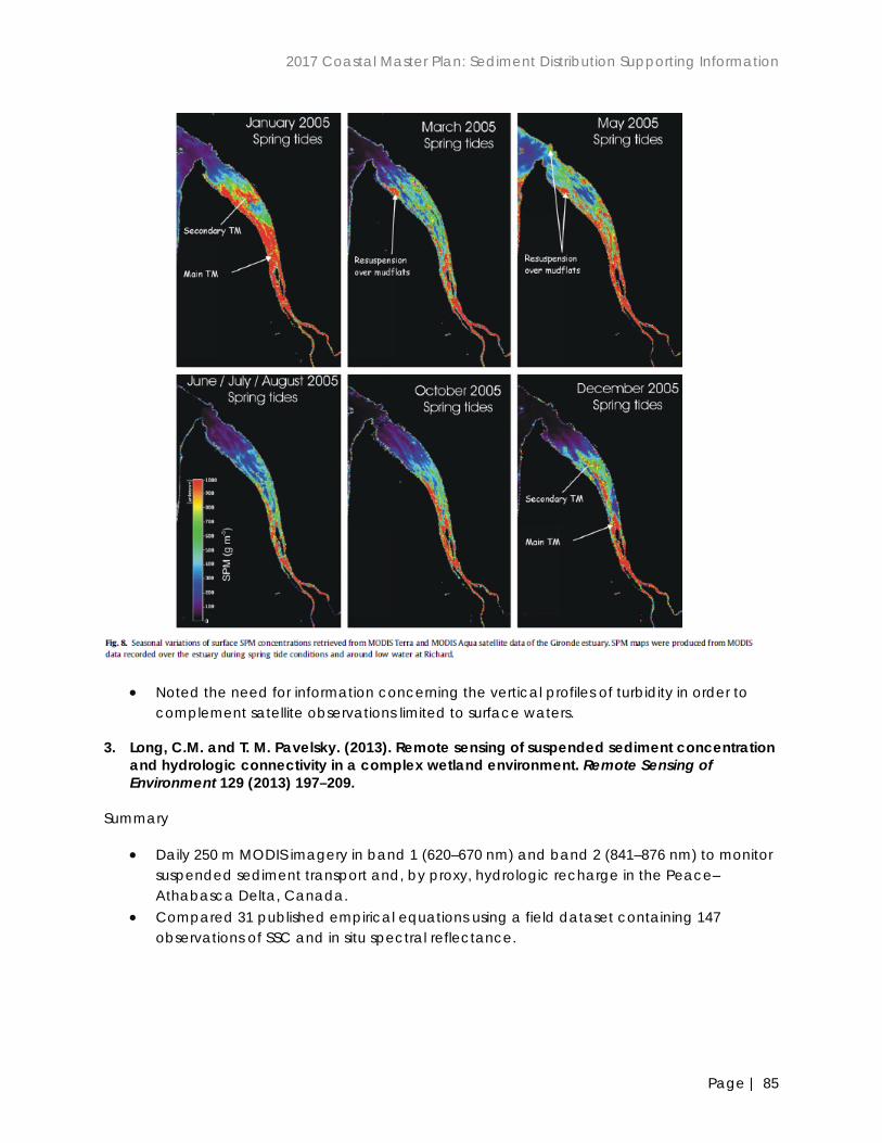
2017 Coastal Master Plan: Sediment Distribution Supporting Information
Page | 85
• Noted the need for information concerning the vertical profiles of turbidity in order to complement satellite observations limited to surface waters.
3. Long, C.M. and T. M. Pavelsky. (2013). Remote sensing of suspended sediment concentration and hydrologic connectivity in a complex wetland environment. Remote Sensing of Environment 129 (2013) 197–209.
Summary
• Daily 250 m MODIS imagery in band 1 (620–670 nm) and band 2 (841–876 nm) to monitor suspended sediment transport and, by proxy, hydrologic recharge in the Peace–Athabasca Delta, Canada.
• Compared 31 published empirical equations using a field dataset containing 147 observations of SSC and in situ spectral reflectance.

2017 Coastal Master Plan: Sediment Distribution Supporting Information
Page | 86
• Results suggest potential for spatial transferability of such models, but success is contingent on the equation meeting certain criteria: 1) use of a near infrared band in combination with at least one visible band, 2) development based on SSCs similar to those in the observed region, and 3) a nonlinear form.
• Results suggest that models developed using comparatively low SSCs have limited success predicting the higher SSCs.
• Found that it is possible to qualitatively predict SSCs using models developed elsewhere. • Several models produce estimates of SSC that are highly correlated with validation
dataset, and these models can be adapted using in situ measurements to quantitatively predict SSCs.

2017 Coastal Master Plan: Sediment Distribution Supporting Information
Page | 87
4. Martinez, J. M., Guyot, J. L., Filizola, N., & Sondag, F. (2009). Increase in suspended sediment discharge of the Amazon River assessed by monitoring network and satellite data. Catena, 79(3), 257-264.
Summary
• Quantification of the Amazon River sediment budget which has been assessed by looking at data from a suspended sediment discharge monitoring network and remote sensing estimates derived from MODIS spaceborne sensor.
• Surface suspended sediment concentration has been sampled every 10 days since 1995. • Remote sensing reflectance is derived from continuous time series of 554 MODIS images
available since 2000 and calibrated with the HYBAM field measurements. • Discharge shows a weak correlation with the suspended sediment concentration during
the annual hydrological cycle, preventing us from computing sediment discharge directly from the water discharge.
• Comparisons of annual sediment discharge assessed using both field and satellite datasets show a very good agreement with a mean difference lower than 1%.
5. Miller, R. L., & McKee, B. A. (2004). Using MODIS Terra 250 m imagery to map concentrations of total suspended matter in coastal waters. Remote Sensing of Environment, 93(1–2), 259–266. http://dx.doi.org/10.1016/j.rse.2004.07.012.
Summary
• Utility of MODIS 250 m data for analyzing complex coastal waters was examined in the Northern Gulf of Mexico.
• Used the MOD02QKM product. • The processing of such data requires at least three successive steps: 1) geolocation using
fields provided at 1 km, 2) atmospheric correction; and 3) conversion into percent surface reflectance.
• A robust linear relationship was established between band 1 (620–670 nm) MODIS Terra 250 m data and in situ measurements of TSM (r2=0.89; n=52; MSE=4.74) acquired during six field campaigns.

2017 Coastal Master Plan: Sediment Distribution Supporting Information
Page | 88
• Results are potential applicable due to the study area overlapping with the study area of
this effort.
2017 Coastal Master Plan: Sediment Distribution Supporting Information
Page | 89
• This study demonstrates that the moderately high resolution of MODIS 250 m data and the operating characteristics of the instrument provide data useful for examining the transport and fate of materials in coastal environments, particularly smaller bodies of water such as bays and estuaries.
6. Nechad, B., Ruddick, K.G., & Y. Park. (2010). Calibration and validation of a generic multisensor algorithm for mapping of total suspended matter in turbid waters. Remote Sensing of Environment 114 (2010) 854–866.
Summary
• A TSM algorithm is developed here for turbid waters, suitable for any ocean color sensor including MERIS, MODIS and SeaWiFS.
• Hyperspectral calibration is made using seaborne TSM and reflectance spectra collected in the southern North Sea.
• Two versions of the algorithm are considered: one which gives directly TSM from reflectance, the other uses the reflectance model of Park and Ruddick (2005) to take account of bidirectional effects.
• Applying a nonlinear regression analysis to the calibration data set gave relative errors in TSM estimation less than 30% in the spectral range 670–750 nm.
• Validation of this algorithm for MODIS and MERIS retrieved reflectances with concurrent in situ measurements gave the lowest relative errors in TSM estimates, less than 40%, for MODIS bands 667 nm and 678 nm and for MERIS bands 665 nm and 681 nm.
7. Petus, C., Chust, G., Gohin,F., Doxaran,D., Froidefond, J., & Y. Sagarminaga (2010). Estimating turbidity and total suspended matter in the Adour River plume (South Bay of Biscay)using MODIS 250-m imagery. Continental Shelf Research 30; 379–392.
Summary
• The results obtained show that MODIS-Aqua band1, at 250-m resolution and atmospherically corrected, is appropriate to retrieve turbidity and TSMc using the following second-order polynomial regression models: TMSc=12,450x2+666.1x+0.48 and Turb.=26,110x2+604.5x+0.24.
• In spite of high correlations observed between Rrs(B2)sim andTurb.in-situ (TSMcin-situ), they found that MODIS-Aqua band2 is not sensitive enough to detect turbidity(TSMc)variations between 0.01 and 10 NTU (mg/l).
8. Villar,R.E., Martinez J.M., Texier,M.L., Guyot, J.L., Fraizy,P., Meneses, P.R., & E. de Oliveira. (2013). A study of sediment transport in the Madeira River, Brazil, using MODIS remote-sensing images. Journal of South American Earth Sciences 44 (2013) 45-54.
Summary
• MODIS space-borne sensors were used to analyze the suspended sediment transport processes along the main stem of the Madeira River.
• Field measurements of suspended sediment concentration, spectral radiometry and granulometry were performed.
2017 Coastal Master Plan: Sediment Distribution Supporting Information
Page | 90
• The relationship between the spectral reflectance and the surface suspended sediment concentration (SSSC) was analyzed using both field radiometric measurements and satellite data.
• Satellite reflectance was found to be significantly correlated with the SSSC. However, a seasonal dependency was demonstrated, most likely caused by a variable granulometric distribution along the annual cycle.
• The ratio between the red and near-infrared bands was found to be free of the seasonal dependency (r ¼ 0.79, N ¼ 282), and a SSSC retrieval model was built from the satellite data.
• The satellite retrieved SSSC time series showed excellent accuracy over the 11-year period and at two different stations.
9. Wang, F., Zhou, B., Xu, J., Song, L., & Wang, X. (2009). Application of neural network and MODIS 250 m imagery for estimating suspended sediments concentration in Hangzhou Bay, China. Environmental geology, 56(6), 1093-1101.
Summary
• An ANN model to simulate the relationship between surface water SSC and satellite-received radiances was employed.
• In situ SSC measurements from the Hangzhou Bay were used for calibration. • Significant correlations were observed between in situ measurements and band 1–2
reflectance values of MODIS images, respectively. • Results indicated that application of ANN model with one hidden layer appeared to
yield superior simulation performance (r2 = 0.98; n = 25) compared with regression analysis method.
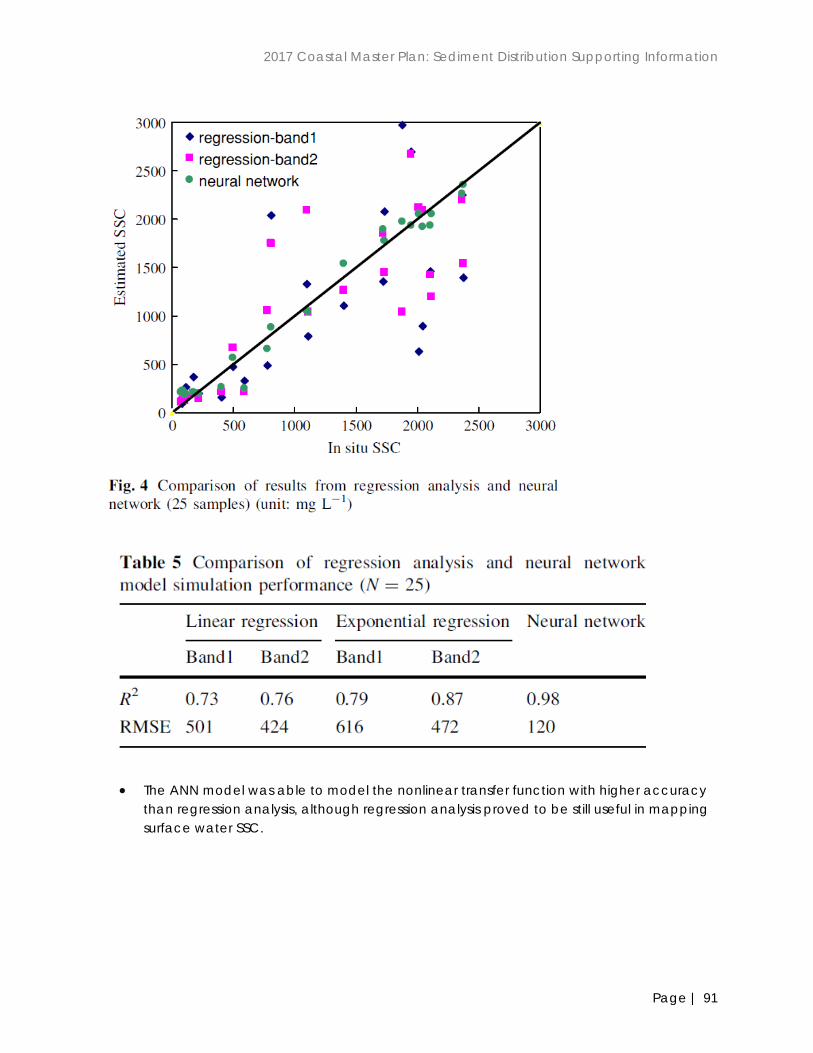
2017 Coastal Master Plan: Sediment Distribution Supporting Information
Page | 91
• The ANN model was able to model the nonlinear transfer function with higher accuracy than regression analysis, although regression analysis proved to be still useful in mapping surface water SSC.
2017 Coastal Master Plan: Sediment Distribution Supporting Information
Page | 92
6.0 Calibration/Validation of Suspended Sediment Using Remote Sensing
The purpose of this section is to propose a procedure for model calibration and/or validation. Since there are insufficient TSS datasets to validate a coast wide sediment subroutine, the team decided to investigate the use of imagery from remotely sensed data. For example, reflectance from satellite images can provide synoptic patterns of TSS for the entire coast; these reflectance values can be calibrated to the limited suspended solids data that are available, and the calibrated reflectance-TSS correlations can be used to convert the reflectance values to TSS maps. Landsat and MODIS satellite sensors have been used in the past to successfully quantify suspended sediment concentrations in coastal waters (Miller et al., 2005; Georgiou et al., 2007; Zhao et al., 2011). Multiple techniques/algorithms have been applied to turn reflectance values into meaningful information. Landsat MSS (60 m) and Landsat TM (30 m) provide valuable information for coastal researchers at higher spatial resolutions as compared to Moderate Resolution Imaging Spectroradiometer (MODIS, 250 m) imagery while MODIS imagery provides a much larger swath (2330 km) as compared to Landsat (185 km).
Various combinations of bands or band ratios are used to model these relationships. Factors such as sediment grain size, chlorophyll, and dissolved organic matter strongly affect a water body’s spectral characteristics and therefore the usefulness of these techniques. To account for these water column properties requires site specific relationships data on reflectance and TSS. Methods which utilize Landsat imagery involve large amounts of in situ ground truthing around the time of satellite overpass. MODIS uses daily time-series imagery at low spatial resolution (250 m) over large areas (2,330 km) and field collection over a lengthy period is recommended for calibration of TSS and reflectance. One method of avoiding the collection of excessive field data was applied by Rouse and Coleman (1976) who used Landsat imagery to map the sediment plume around the Mississippi Delta. They used laboratory measured reflectances to calibrate the satellite data to suspended solids concentration.
Many linear and nonlinear regressions have been proposed for correlating field measured water quality parameters (TSS or turbidity) and satellite reflectances (e.g., Dekker et al., 2002; Doxaran et al., 2003, Fraser, 1998; Harrington et al., 1992; Islam et al., 2001; Ritchie & Cooper,1991; Mertes et al., 1993).
An example of the linear regression is reported by Hadjimitsis et al. (2006) using Landsat 5-TM and Landsat-7 (ETM+) and measured turbidity within a reservoir in Cyprus. This study led to the regression equation 52 for determining turbidity:
𝑝 = 0.0034(𝑇𝑢𝑟𝑇𝑖𝜋𝑖𝑑𝑇 𝑖𝑖 𝑁𝑇𝑈) + 0.0058 (48) where: 𝑝 = reflectance. Topliss et al. (1990) provided an example of a nonlinear regression using Landsat data in the form of Equation 49.
ln(𝑆𝑢𝑟𝑖𝑆𝑣𝑆 𝑆𝑢𝑠𝑝𝑆𝑖𝜋𝑆𝜋 𝑆𝑆𝑆𝑖𝜋𝑠,𝑚𝑔/𝐿) = −9.21𝑅1 2⁄ + 2.71𝑅1 2⁄2 + 8.45 (49)
where: R1/2 = ratio of MDD band 1 to band 2 reflectances. Keiner and Yan (1998) applied a neural network to model the relationship between sediment concentrations and satellite radiances from the Landsat TM for Delaware Bay using three visible

2017 Coastal Master Plan: Sediment Distribution Supporting Information
Page | 93
Landsat TM bands and were able to model the relationship better than a traditional regression analysis. In coastal waters, sediments and dissolved organic matter strongly affect the water body’s spectral characteristics. Because of this, in situ data must be collected at the time of satellite overpass and sometimes this must be done for separate seasons to account for variations. Regression analysis is the typical method for modeling relationships between field measured water quality and satellite reflectances. Various combinations of bands or band ratios are used to model these relationships. The best combination for sediment was the log-linear equation using only band three. Neural networks have the ability to model nonlinear behavior. These models are trained and use weights and biases in order to best model the data. Neural networks out-performed regression analysis. The researchers recommend that future studies include more in situ samples for training of the neural network which should include multidate analysis. At least 30 samples should be obtained with a wide range of values. Neural networks are excellent interpolators but not great at extrapolating in ranges outside the training set. It would be more difficult to apply this approach in the ICM calibration than in a regression relationship.
The use of a reflectance from MODIS imagery has been used to track the plumes from the Bonnet Carré Spillway opening in 1997 (Haralampides, 2000). Miller et al. (2005) used MODIS reflectance and field TSS samples to derive a resuspension potential for Lake Pontchartrain. Georgiou et al. (2007) calibrated an ECOMSED model for Lake Pontchartrain using MODIS imagery. The circulation and wave generated sediment processes were included in this ECOMSED model used by Georgiou et al. (2007); the dominant forcing was found to be wind waves and current rather than tide. Since the open water areas of coastal Louisiana are generally shallow, the impact of wind-wave induced resuspension is a major factor in the sediment distribution in open waters. The proposed compartmental sediment model for the open water areas is similar to the one that Georgiou et al. (2007) applied to Lake Pontchartrain. The most useful form of this imagery is medium to long term averages by month.
6.1 Potential Uses
Previous investigations have revealed patterns of (see figure below). The preliminary results of this investigation are seen below:
Average Landsat band 3 reflectance values (1984-2010). (Allen et al., 2012)
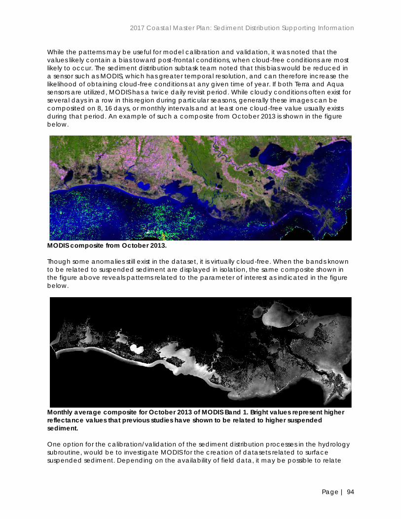
2017 Coastal Master Plan: Sediment Distribution Supporting Information
Page | 94
While the patterns may be useful for model calibration and validation, it was noted that the values likely contain a bias toward post-frontal conditions, when cloud-free conditions are most likely to occur. The sediment distribution subtask team noted that this bias would be reduced in a sensor such as MODIS, which has greater temporal resolution, and can therefore increase the likelihood of obtaining cloud-free conditions at any given time of year. If both Terra and Aqua sensors are utilized, MODIS has a twice daily revisit period. While cloudy conditions often exist for several days in a row in this region during particular seasons, generally these images can be composited on 8, 16 days, or monthly intervals and at least one cloud-free value usually exists during that period. An example of such a composite from October 2013 is shown in the figure below.
MODIS composite from October 2013. Though some anomalies still exist in the dataset, it is virtually cloud-free. When the bands known to be related to suspended sediment are displayed in isolation, the same composite shown in the figure above reveals patterns related to the parameter of interest as indicated in the figure below.
Monthly average composite for October 2013 of MODIS Band 1. Bright values represent higher reflectance values that previous studies have shown to be related to higher suspended sediment. One option for the calibration/validation of the sediment distribution processes in the hydrology subroutine, would be to investigate MODIS for the creation of datasets related to surface suspended sediment. Depending on the availability of field data, it may be possible to relate
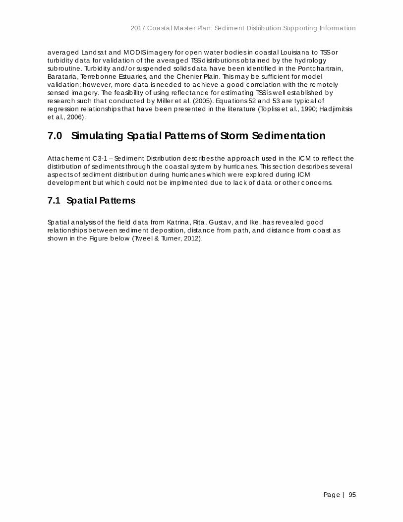
2017 Coastal Master Plan: Sediment Distribution Supporting Information
Page | 95
averaged Landsat and MODIS imagery for open water bodies in coastal Louisiana to TSS or turbidity data for validation of the averaged TSS distributions obtained by the hydrology subroutine. Turbidity and/or suspended solids data have been identified in the Pontchartrain, Barataria, Terrebonne Estuaries, and the Chenier Plain. This may be sufficient for model validation; however, more data is needed to achieve a good correlation with the remotely sensed imagery. The feasibility of using reflectance for estimating TSS is well established by research such that conducted by Miller et al. (2005). Equations 52 and 53 are typical of regression relationships that have been presented in the literature (Topliss et al., 1990; Hadjimitsis et al., 2006).
7.0 Simulating Spatial Patterns of Storm Sedimentation
Attachement C3-1 – Sediment Distribution describes the approach used in the ICM to reflect the distirbution of sediments through the coastal system by hurricanes. This section describes several aspects of sediment distribution during hurricanes which were explored during ICM development but which could not be implmented due to lack of data or other concerns.
7.1 Spatial Patterns
Spatial analysis of the field data from Katrina, Rita, Gustav, and Ike, has revealed good relationships between sediment deposition, distance from path, and distance from coast as shown in the Figure below (Tweel & Turner, 2012).

2017 Coastal Master Plan: Sediment Distribution Supporting Information
Page | 96
Distribution of mineral sediments with distance from storm path and distance from coastline (Tweel & Turner, 2012). Three storms are presented: Katrina (dotted line); Rita (bold dashed line); Gustav (chain dashed line). The top panels (A, B) show cumulative deposition and bottom panels (C, D) show deposition within each 10 km interval, plotted at the midpoint. The panels at left (A, C) show distance from path and the panels at right (B, D) show distance from coast. Deposition is based on spatially interpolated sediment distribution measured at 10 km increments. Deposition is measured east of the storm path for Gustav, Rita, and Ike, and on both sides for Katrina because of the distinct distribution of sediment. The data for Hurricane Ike in panel C is for the Louisiana portion of the deposition footprint; Texas is excluded.
These spatial patterns of sediment distribution could be incorporated into the 2017 ICM. Tweel and Turner (2012) found better relationships with “distance from coast” than those of “distance from path”, noting that "there are remarkably consistent depositional patterns along a shoreline-to-inland gradient. These patterns were more variable with distance from the path". However, the mechanisms driving these patterns are unclear. Both observations and modeling of storm

2017 Coastal Master Plan: Sediment Distribution Supporting Information
Page | 97
effects on water level (e.g., Cobell et al., 2013) show complex patterns of inundation often related to storm track. While specific relationships for storm sediment deposition related to multiple factors have yet to be developed based on empirical data, they may be appropriate for the ICM.
The data used to construct panels A and B from the Figure above was made available by the authors. This then enabled the calculation of generalized formulas which could be used in the ICM. For example, cumulative deposition by distance from coast was calculated for three storms (Katrina, Rita, and Gustav), and an exponential rise to maximum equation was calculated (see Figure below).
Distance Inland vs. Cumulative % of Total Deposition (Katrina, Rita, and Gustav). Adapted from Figure 3b in Tweel & Turner (2012). Ike is excluded as deposition was not measured in Texas. A similar equation was calculated for cumulative deposition by distance from path and an exponential rise to maximum equation was calculated (see below).

2017 Coastal Master Plan: Sediment Distribution Supporting Information
Page | 98
Distance from Path vs. Cumulative % of Total Deposition (Katrina, Rita, and Gustav). Adapted from Figure 3a in Tweel & Turner (2012). Ike is excluded as deposition was not measured in Texas. Tweel and Turner (2014) developed a model based on data collected for three storms and used it to estimate the average deposition on the deteriorating Louisiana coast from 1851 to 2008. They use a relationship based on only three storms which may not be sufficiently reliable for application to the storm conditions to be used in the ICM. 7.2 Total Sediment Load
These equations (outlined in the figures above) would have to be applied to a total sediment load to be distributed. Tweel and Turner (2012) includes the best data available to determine total load but is limited to only 3 major storms. It is possible that a relationship exists between some characteristic or characteristics of storms and total sediment load deposited; however, there is not sufficient literature to establish such a relationship. If the average of the three storms (Katrina, Rita, and Gustav) described in Tweel and Turner (2012) was used, 45.5 MMT would be applied to all storms category 3 or higher, and then distributed according to the methodology outlined below and based on the equations above.

2017 Coastal Master Plan: Sediment Distribution Supporting Information
Page | 99
7.3 Spatial Distribution of Sediment
Buffers could be calculated from shoreline and from the path of storms used to drive the ICM for broad intervals (0-5 km, 5-10 km, etc.). The equations outlined above could then be used to determine the percentage of sediment which is deposited in each zone. A generalized representation of these buffers is shown below.
Generalized Visual Representation of a Potential Methodology. Buffers shown were established at intervals from a generalized coastline and from the track of the storm, those layers would then be intersected and the amount of sediment to be deposited in each zone calculated.

2017 Coastal Master Plan: Sediment Distribution Supporting Information
Page | 100
8.0 Additional Literature Cited
Allen, Y.C., Couvillion, B. R., & Barras, J.A. (2012) Using multitemporal remote sensing imagery and inundation measures to improve land change estimates in coastal wetlands. Estuaries and Coasts, 35 (1), 190-200.
Cobell, Z., Zhoa, H., Roberts, H.J., Clark, R., & Zou, S. (2013). Surge and wave modeling for the
Louisiana 2012 Coastal Master Plan. In: Peyronnin, N. and Reed, D. (eds.), Louisiana’s 2012 Coastal Master Plan Technical Analysis. Journal of Coastal Research, Special Issue 67, 88–108.
Dietrich, J.C., Zijlema, M., Westerink, J.J., Holthuijsen, L.H., Dawson, C.N., Luettich, R.A., Jensen,
R.E., Smith, J.M., Stelling, G.S., & Stone, G.W. (2011). Modeling hurricane waves and storm surge using integrally-coupled, scalable computations. Coastal Engineering, 58(1), 45–65.
Dekker, A.G., Vos, R.J., & Peters, S.W.M. (2002). Analytical algorithms for lake water TSM
estimation for retrospective analyses of TM and SPOT sensor data. International Journal of Remote Sensing, 23(1), 5-35.
Dibajnia, M., & Watanabe, A. (1996). A transport rate formula for mixed-size sands. Coastal
Engineering Proceedings, 1(25). Doxaran, D., Froidefond, J.M., & Castaing, P. (2003). Remote-sensing reflectance of turbid
sediment-dominated waters. Reduction of sediment type variations and changing illumination conditions effects by use of reflectance ratios. Applied Optics, 42(15), 2623-2634.
Doyle, R.D. (2001). Effects of waves on the early growth of Vallisneria Americana. Freshwater
Biology, 46(3), 389–397. Foote, A. L., & Kadlec, J.A. (1988). Effects of wave energy on plant establishment in shallow
lacustrine wetlands. Journal of Freshwater Ecology, 4(4), 523-532. Gailani, J., Ziegler, C.K., & Lick, W. (1991). Transport of suspended solids in the Lower Fox
River. Journal of Great Lakes Research, 17(4), 479-494. Galinato, M.I., & Van der Valk, A.G. (1986). Seed germination traits of annuals and emergents
recruited during drawdowns in the Delta Marsh, Manitoba, Canada. Aquatic Botany, 26, 89-102.
Georgiou, I., McCorquodale, A. & Crowder, K. (2007). Rapid prototyping of NASA MODIS 250 m
data in the calibration/validation of a sediment transport model for water quality assessment and public health decision support. Report Submitted to Richard Miller, Ph.D. National Aeronautics and Space Administration Science and Technology Division EA41. Stennis Space Center, MS 39529.
Haihong, Z., Chen, Q., Walker, N.D., Zheng, Q., & MacIntyre, H.L. (2011). A study of sediment
transport in a shallow estuary using MODIS imagery and particle tracking simulation, International Journal of Remote Sensing, 32, 6653-6671.
2017 Coastal Master Plan: Sediment Distribution Supporting Information
Page | 101
Haralampides, K. (2000). A study of the hydrodynamics and salinity regimes of the Lake Pontchartrain system. New Orleans, Louisiana: University of New Orleans (Doctoral dissertation, Doctoral thesis, 219p).
Hellestrom, T. 1991. The effect of sediment resuspension on algal production in a shallow lake.
Hydrobiologia. 213, 183-190 HydroQual Inc. (2002). A primer for ECOMSED. User’s Manual, Ver. 1.3. HydroQual Inc., Mahwah,
NJ, pp. 188. Kineke, G.C., Sternberg, R.W., Trowbridge, J.H., & Geyer, W.R. (1996). Fluid-mud processes on the
Amazon continental shelf. Continental Shelf Research, 16(5), 667-696. Lawson, S.E., Wiberg, P.L., McGlathery, K.J., & Fugate, D.C. (2007). Wind-driven sediment
suspension controls light availability in a shallow coastal lagoon. Estuaries and Coasts, 30(1), 102-112.
Lee, S.C., & Mehta, A.J. (1994). Cohesive Sediment Erosion. University of Florida, Gainesville.
Department of Coastal and Oceanographic Engineering. Miller, R.L., McKee, B.A., & D'sa, E.J. (2005). Monitoring bottom sediment resuspension and
suspended sediments in shallow coastal waters. Remote Sensing of Coastal Aquatic Environments, 259-276.
Möller, I., Spencer, T., French, J. R., Leggett, D.J., & Dixon, M. (1999). Wave transformation over
salt marshes: a field and numerical modelling study from North Norfolk, England. Estuarine, Coastal and Shelf Science, 49(3), 411-426.
Munday, J.C., & Alföldi, T.T. (1979). Landsat test of diffuse reflectance models for aquatic
suspended solids measurement. Remote sensing of environment, 8(2), 169-183. Munk, W.H., & Anderson, E.R. (1948). Notes on a theory of the thermocline. Journal of Marine
Research, 3, 276–295. Park, Y.J., & Ruddick, K. (2005). Model of remote-sensing reflectance including bidirectional
effects for case 1 and case 2 waters. Applied Optics, 44(7), 1236-1249. Partheniades, E. (1990). Microstructure of fine-grained sediments: from mud to shale. Frontiers in
Sedimentary Geology. Springer-Verlag, Berlin, 175-183. Phillips, O.M. (1966). The Dynamics of the Upper Ocean, Cambridge University Press, Cambridge.
pp. 216. Sheng, Y.P. & Lick, W. (1979). The transport and resuspension of sediments in a shallow lake.
Journal of Geophysical Research, 84, 1809–1826. Tweel, A.W., & Turner, R.E. (2014) Contribution of tropical cyclones to the sediment budget for
coastal wetlands in Louisiana, USA. Land scape Ecology, 29(6), 1083-1094. van Ledden, M. (2003). Sand-mud segregation in estuaries and tidal basins (p. 221). University of
Technology, Delft.
2017 Coastal Master Plan: Sediment Distribution Supporting Information
Page | 102
Van Rijn, L.C. (1993). Principles of sediment transport in rivers, estuaries and coastal seas (Vol. 1006). Amsterdam: Aqua publications.
van Rijn, L.C. (1984). Sediment Transport, Part II: Suspended load transport. Journal of Hydraulic
Engineering, ASCE, 11. Whitehouse, R.J. S., Bassoullet, P., Dyer, K.R., Mitchener, H.J., & Roberts, W. (2000). The influence
of bedforms on flow and sediment transport over intertidal mudflats. Continental Shelf Research, 20(10), 1099-1124.
Ziegler, C.K., & Nisbet, B. (1994). Fine-grained sediment transport in Pawtuxet River, Rhode
Island. Journal of Hydraulic Engineering, 120(5), 561-576. Ziegler, C.K., & Nisbet, B.S. (1995). Long-term simulation of fine-grained sediment transport in
large reservoir. Journal of Hydraulic Engineering, 121(11), 773-781.