attachment d9 - the fundÃo tailings dam...
TRANSCRIPT

Fundão Tailings Dam Review Panel
Report on the Immediate Causes of the Failure of the Fundão Dam Appendix D – Laboratory Geotechnical Data and Interpretation
August 25, 2016
ATTACHMENT D9 University of Alberta Sedimentation/Consolidation Test on Slimes

1
Large Strain Consolidation Testing of
Flotation Tailings
Prepared for
Klohn Crippen Berger
Prepared by
Louis K. Kabwe, Ph.D.
Research Associate
and
Ward G. Wilson, Ph.D., P.Eng., P.Geol., FCAE
Principle Investigator
June 2016

2
Table of Contents
Table of Contents…………………………………………………………………………… 2
List of Tables (Main body)………………………………………………………………… 3
List of Figures (Main body)…………………………………………………………. 3
List of Figures in Appendix A……………………………………………………… 3
List of Tables in Appendix B………………………………………………………. 3
List of Figures in Appendix C………………………………………………………. 3
1. Introduction………………………………………………………………………… 4
2 Tailings Sample……………………………………………………………………. 4
3. Large Strain Consolidation Test…………………………………………………. 4
3.1 Large Strain Consolidation Apparatus ……………………………………………… 5
3.2 Determination of End of Consolidation ……...……………………………………... 5
3.3 Hydraulic Conductivity Test………………………………………………………… 7
3.4 Shear Strength Test………………………………………………………………….. 8
4. Summary of Results……………………………………………………………….. 9
5. Observations ………………………………………………………………………. 12
APPENDICES
Appendix A Large Strain Consolidation Test Setup.…………………………………. 13
Appendix B Sample Water Chemistry……………………………………………….. 15
Appendix C Time – Settlement and Pore Pressure Dissipation Plots………………… 18
List of Tables (main body)
Table 1: Measured Large Strain Consolidation Properties of Tailings Sample…..... 9
Table 2: Tailings Sample Properties………………………………………………… 10
3
List of Figures (main body)
Figure 1: Large strain consolidation set up…………………………………………... 5
Figure 2: Typical large strain consolidation time-settlement curve ……………….... 6
Figure 3: Typical excess pore pressure dissipation curve.…………………………... 6
Figure 4: Set up of hydraulic conductivity measurement……………………………. 7
Figure 5: Compressibility plot (void ratio versus effective stress)............................... 11
Figure 6: Permeability plot (hydraulic conductivity versus void ratio)…………….... 11
List of Figures in Appendix A
Figure A1 Schematic set up of the large strain consolidation test, step 1…………….. 14
Figure A2 Schematic set up of the large strain consolidation test, step 2…………….. 14
Figure A3 Schematic set up of the large strain consolidation test, step 3…………….. 14
List of Tables in Appendix B
Table B1 Anions concentrations in tailings water sample…………………………… 16
Table B2. Cations concentrations in tailings Water sample…………………………. 16
Table B3. Other water chemistry in tailings water sample…………………………… 17
List of Figures in Appendix C
Time – settlement and excess pore pressure dissipation plots…………………………… 19

4
1. INTRODUCTION
Klohn Crippen Berge contracted the University of Alberta Geotechnical Centre to perform
Large Strain Consolidation (LSC) testing services for Flotation Tailings.
This report consists of two main parts: the main body and the appendices. Detailed data are
presented in tables and figures in appendices. The tables and figures in the main body of the
report summarize the results of the tests, and are briefly discussed. The appendix tables and
figures will not be discussed and are presented so the report includes all data from the testing
program. Large files of measurement data are not included in this report but will be transmitted
to Klohn electronically.
2. TAILINGS SAMPLE
A 15 L container of tailings sample was received from Klohn Crippen Berge for LSC testing
program. The solids content of the sample was measured upon arrival and was found to be
over 76 %. The specific gravity of the sample (3.85) was not measured in this test but was
provided by Klohn. The solids content of the sample was reduced to about 50% by mixing the
sample with distilled water. The decanted water after mixing was used for hydraulic
conductivity measurement at the end of consolidation for each load step. The water chemistry
of the tailings sample was measured and results are presented in Appendix B.
3. LARGE STRAIN CONSOLIDATION TEST
The objectives of the LSC tests are:
• To determine the relationship between effective stress and void ratio.
• To determine the relationship between void ratio and hydraulic conductivity
(permeability of water).

5
3.1 Large Strain Consolidation LSC Apparatus
A LSC test was performed in a standard consolidation apparatus (150 mm dia. x 150 mm high).
The LSC apparatus used in this testing program confines the slurried material so it can be tested
at any water content. The first applied stress, the self-weight of the slurry, can be about 0.3 to 0.5
kPa. Effective stresses up to about 10 kPa were applied by dead loads acting on the piston
(Figure A1 in Appendix A). Effective stresses over 10 kPa were applied in a loading fram by an
air pressure Bellofram. Subsequent loads were approximately doubled for each load step up to
1000 kPa maximum. The setup of the LSC test used at the geotechnical centre of the University
of Alberta is shown in Figures 1 and Figure A1 in Appendix A.
Figure 1. Set up of the large strain consolidation LSC test at the Geotechnical Centre of the
University of Alberta.
3.2 Determination of End of Consolidation
When a load is applied, the progress of the consolidation is evaluated by monitoring the change
in height of the sample (vertical strain) with a LVDT and by measuring the pore pressure at the

6
base of the sample. The load is maintained until the vertical strain/or base pore pressure
dissipation are significantly completed before adding the next load as shown in Figures 1 and 2.
Figure 2. Typical time-settlement curve in LSC test.
Figure 3. Typical excess pore pressure dissipation curve in LSC test.
6.05
6.10
6.15
6.20
6.25
6.30
6.35
6.40
6.45
6.50
0 50 100 150 200 250 300 350
100 kPa
LV
D (
cm)
Time (min)
Time - Settlement Curve
0
10
20
30
40
50
60
0 50 100 150 200 250 300 350
400 kPa
Ex
cess
pore
pre
ssure
(kP
a)
Time (min)
Excess Pore Pressure Dissipation

7
3.3 Hydraulic Conductivity (Permeability) Test
The permeability was measured at the end of consolidation for each load step. An upward flow
constant head test was performed with the head difference h (h=ho-h1) being kept small enough
so that seepage forces will not exceed the applied stress and cause sample fracturing during the
permeability test.
In one dimension, water flows through a fully saturated soil sample in accordance with Darcy’s
empirical law is given by:
ikAq =
or
kiA
qv ==
Where q = volume of water flowing per unit time, A = cross-sectional area of soil sample
corresponding to the flow q, k = coefficient of permeability, i = hydraulic gradient, and v =
discharge velocity. The hydraulic gradient, i, is given by:
Figure 4. Setup of permeability measurement.
l
hh
l
hi o 1
−==
Where
l = the length of the sample.
The inflow is monitored to ensure that steady state flow conditions are obtained. The units of the

8
coefficient of permeability are those of velocity (m/s).
For a given soil, the coefficient of permeability is a function of void ratio. The coefficient of
permeability depends primarily on the average size of the pores, which in turn is related to the
distribution of particles sizes, particle shape and soil structure. The presence of a small
percentage of fines in a coarse-grained soil results in a value of k significantly lower than the
value for the same soil without fines.
3.4 Van Shear Test
The laboratory vane shear test consists of inserting a four-bladed vane in the end of a tube
sample and rotating it at a constant rate to determine the torque required to cause a cylindrical
surface to be sheared by the vane. This torque is then converted to unit shearing resistance of the
cylindrical surface area. The torque is measured by a calibrated torque transducer that is attached
directly to the vane. The undrained shear strength is calculated using the following expression:
T = τ x K
Where:
T = torque, lbf.ft (N.m)
τ = undrained shear strength, lbf/ft2 (Pa), and
K = vane blade constant, ft3 (m3).
T and K are given as follows (assuming the distribution of the shear strength is uniform
across the ends of the failure cylinder and around the perimeter):
+=
=
+=
3
1
2
3
1
2
3
3
v
v
y
y
v
v
D
HDK
K
T
D
HDT
π
τ
τπ
Where:
Dv = measured diameter of the vane, in. (mm),
H = measured height of the vane, in. (mm).

9
4. SUMMARY OF RESULTS
The LSC tests results are summarized in Tables 1 and 2 and in Figures 4 and 5.
Table 1. Summary of measured large strain consolidation properties of tailings sample.
Load Effective
stress
Sample
height
Void
ratio
Hydraulic
conductivity
Solids
content
(kPa) (cm) (m/s) (%)
Self-
weight
settling 0.4 7.0 2.61 7.84E-08 50.0
Load-1 1.1 6.5 2.34 6.67E-08 60.4
Load-2 2.0
6.0 2.08 3.88E-08 63.3
Load-3 2.9
5.8 1.93 3.13E-08 64.9
Load-4 3.8
5.6 1.85 2.87E-08 65.9
Load-5 8.4
5.3 1.67 1.83E-08 68.2
Load-6 13.0
5.0 1.53 1.33E-08 70.0
Load-7 30
4.6 1.27 6.97E-09 73.8
Load-8 100
4.2 1.08 3.66E-09 76.9
Load-9 200
4.1 1.02 2.43E-09 77.9
Load-10 400
3.9 0.94 2.22E-09 79.1
Load-11 600
3.8 0.89 1.83E-09 80.0
Load-12 1000
3.7 0.83 1.21E-09 81.1

10
Table 2. Summary of tailings sample properties.
Tailings sample
(Gs = 3.85)
Initial
(prior to
consolidation)
Final
(after 1000 kPa
effective stress)
Solids content
(oven-dry) (%)
50
82
Void ratio
(oven-dry) 2.61
0.85
Shear strength (kPa)
144

11
Figure 4. Compressibility plot (void ratio vs effective stress) of the tailings sample.
Figure 5. Permeability plot (hydraulic conductivity vs void ratio) of the tailings sample.
0.2
0.6
1.0
1.4
1.8
2.2
2.6
3.0
0 1 10 100 1,000 10,000
Data
Effective stress (kPa)
Void
rat
ioCompressibility Plot
y = 3E-09x3.7106
R² = 0.9965
1.0E-10
1.0E-09
1.0E-08
1.0E-07
1.0E-06
0.0 0.5 1.0 1.5 2.0 2.5 3.0
data
Hydra
uli
c co
nduct
ivit
y (
m/s
)
Void ratio
Permeability Plot

12
5. OBSERVATIONS
Figure 4 shows that the compressibility (the relationship between void ratio e and effective stress
σ’) increases linearly when effective stresses are between 2 and 30 kPa. The compression index
Cc (i.e., the slope of the linear portion of the e-logσ’ curve) is about 0.026.
Figure 5 shows the relationship between hydraulic conductivity k and void ratio e. The k
decreases exponentially as e decreases. The k decreases by one order of magnitude (i.e., from
7.84x10⁻⁸ m/s to 6.97x10⁻⁹ m/s) when e decreases from 2.6 to 1.27. By fitting a mathematical
equation to the data points, it is found that a power law yields the prediction equation with high
correlation coefficient (R2=0.996) for the tailings sample tested.

13
APPENDIX A
Large Strain Consolidation Set Up at the
University of Alberta Geotechnical Centre

14
Figure A1. Initial set up of the large strain consolidation test before loading sample
Figure A2. Sample loaded with piston and dead loads up to about 10 kPa
Figure A3. Sample in loading frame and loaded by Bellofram up to 1000 kPa.

15
APPENDIX B
Tailings Sample Water chemistry

16
Table B1: Anions concentrations in tailings water sample.
mg/L mmol/L mEq/L
fluoride 0.34 1.790E-02 1.790E-02
chloride 5.13 1.447E-01 1.447E-01
nitrite 0.72 1.565E-02 1.565E-02
bromide 0 0 0
sulphate 36.0505 3.753E-01 7.506E-01
nitrate 14.675 2.367E-01 2.367E-01
phosphate 0 0 0
bicarbonate 2.092E+01 3.428E-01 3.428E-01
carbonate 2.417E-03 4.027E-05 8.054E-05
Table B2: Cations concentrations in tailings water sample.
mg/L mmol/L mEq/L
Na23 30.61064 1.331 1.33089739
Mg26 0.0448 1.723E-03 3.446E-03
Si28 1.52866 5.460E-02 2.184E-01
K39 1.96852 5.047E-02 5.047E-02
Ca43 16.67744 3.878E-01 7.507E-01
Ca44 15.9656 3.629E-01
Cr52 0.0072 1.385E-04 4.154E-04
Ni58 0.00302 5.207E-05 2.083E-04
Cu63 0.00206 3.270E-05 6.540E-05
Zn64 0.0152 2.375E-04 4.775E-04
Zn66 0.01584 2.400E-04
Sr86 0.15002 1.744E-03 3.019E-03
Sr88 0.1122 1.275E-03
Mo95 0.00756 7.958E-05 3.133E-04
Mo96 0.0074 7.708E-05
Ba138 0.00634 4.594E-05 9.188E-05

17
Table B3: Other tailings water chemistry (OH- & H+)
mmol/L mEq/L mEq/L
OH- 2.512E-05 2.512E-05 negative
-
1.508422783
H+ 3.981E-04 3.981E-04 positive 2.358889696
difference 0.850466913

18
APPENDIX C
Time – Settlement Plots and
Excess Pore Pressure Dissipation Plots for the
Large Strain Consolidation LSC Test

19
Figure C1. Time – settlement curve for 1.12 kPa effective stress.
Figure C2: Excess pore pressure dissipation for 1.12 kPa effective stress.
1.52.02.53.03.54.04.55.05.56.06.57.0
0 1000 2000 3000 4000 5000 6000
1.12 kPa
LV
DT
(m
m)
Time (min)
Time - Settlement Curve
-0.05
0.00
0.05
0.10
0.15
0.20
0.25
0.30
0.35
0 1000 2000 3000 4000 5000 6000
1.12 kPa
Ex
cess
pore
pre
ssure
(kP
a)
Time (min)
Excess Pore Pressure Dissipation

20
Figure C3. Time – settlement curve for 2.02 kPa effective stress.
Figure C4: Excess pore pressure dissipation for 2.02 kPa effective stress.
-2.5-2.0-1.5-1.0-0.50.00.51.01.52.02.53.0
0 500 1000 1500 2000 2500 3000
2.02 kPa
LV
DT
(m
m)
Time (min)
Time Settlement Curve
0.00
0.05
0.10
0.15
0.20
0.25
0.30
0.35
0.40
0 500 1000 1500 2000 2500 3000
2.02 kPa
Pore
pre
ssure
(kP
a)
Time (min)
Excess Pore Pressure Dissipation

21
Figure C5. Time – settlement curve for 2.92 kPa effective stress.
Figure C6: Excess pore pressure dissipation for 2.92 kPa effective stress.
1.0
1.5
2.0
2.5
3.0
3.5
4.0
4.5
5.0
0 400 800 1200 1600 2000 2400
2.92 kPa
LvD
T (
mm
)
Time (min)
Time - Settlement Curve
0.0
0.2
0.4
0.6
0.8
1.0
1.2
0 400 800 1200 1600 2000 2400
2,92 kPa
Pore
pre
ssure
(kP
a)
Time (min)
Excess Pore Pressure Dissipation

22
Figure C7. Time – settlement curve for 3.82 kPa effective stress.
Figure C8: Excess pore pressure dissipation for 3.82 kPa effective stress.
-1.5
-1.3
-1.1
-0.9
-0.7
-0.5
-0.3
-0.1
0.1
0.3
0 1000 2000 3000 4000 5000 6000
3.82 kPa
LV
DT
(m
m)
Time (min)
Time - Settlement Curve
0.00
0.05
0.10
0.15
0.20
0.25
0.30
0 1000 2000 3000 4000 5000 6000
3.82 kPa
Ex
cess
pore
pre
ssure
(kP
a)
Time (min)
Excess Pore Pressure Dissipation

23
Figure C9. Time – settlement curve for 8.42 kPa effective stress.
Figure C10: Excess pore pressure dissipation for 8.42kPa effective stress.
-1.0-0.6-0.20.20.61.01.41.82.22.63.0
0 500 1000 1500 2000 2500
8.42 kPa
Time (min)
Time - Settlement Curve
LV
DT
(m
m)
-0.20.0
0.20.40.60.81.01.21.4
1.61.8
0 500 1000 1500 2000 2500
8.42 kPa
Ex
cess
pore
pre
ssure
(kP
a)
Time (min)
Excess Pore Pressure Dissipation

24
Figure C11. Time – settlement curve for 30 kPa effective stress.
Figure C12: Excess pore pressure dissipation for 30 kPa effective stress.
6.4
6.5
6.6
6.7
6.8
6.9
7
0 200 400 600 800 1000 1200 1400
30 kPa
LV
DT
(cm
)
Time (min)
Time - Settlement Curve
-0.001
0
0.001
0.002
0.003
0.004
0.005
0.006
0 200 400 600 800 1000 1200 1400
30 kPa
Ex
cess
pore
pre
ssure
(kP
a)
Time (min)
Excess Pore Pressure Dissipation
25
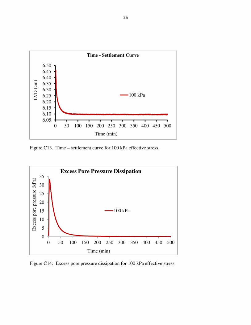
Figure C13. Time – settlement curve for 100 kPa effective stress.
Figure C14: Excess pore pressure dissipation for 100 kPa effective stress.
6.05
6.10
6.15
6.20
6.25
6.30
6.35
6.40
6.45
6.50
0 50 100 150 200 250 300 350 400 450 500
100 kPa
LV
D (
cm)
Time (min)
Time - Settlement Curve
0
5
10
15
20
25
30
35
0 50 100 150 200 250 300 350 400 450 500
100 kPa
Ex
cess
pore
pre
ssure
(kP
a)
Time (min)
Excess Pore Pressure Dissipation

26
Figure C15. Time – settlement curve for 200 kPa effective stress.
Figure C16: Excess pore pressure dissipation for 200 kPa effective stress.
7.88
7.90
7.92
7.94
7.96
7.98
8.00
8.02
8.04
0 200 400 600 800 1,000 1,200 1,400 1,600
200 kPa
LV
D (
mm
)
Time (min)
Time - Settlement Curve
-0.010
0.000
0.010
0.020
0.030
0.040
0.050
0.060
0 200 400 600 800 1000 1200 1400 1600
200 kPa
Ex
cess
pore
pre
ssure
(kP
a)
Time (min)
Excess Pore Pressure Dissipation

27
Figure C17. Time – settlement curve for 400 kPa effective stress.
Figure C18: Excess pore pressure dissipation for 400 kPa effective stress.
7.767.787.807.827.847.867.887.907.927.947.96
0 250 500 750 1,000 1,250 1,500
400 kPa
LV
D (
cm)
Time (min)
Time - Settlement Curve
0
10
20
30
40
50
60
0 250 500 750 1000 1250 1500
400 kPa
Ex
cess
pore
pre
ssure
(kP
a)
Time (min)
Excess pore pressure Dissipation

28
Figure C19. Time – settlement curve for 600 kPa effective stress.
Figure C20: Excess pore pressure dissipation for 600 kPa effective stress.
7.14
7.16
7.18
7.20
7.22
7.24
7.26
0 250 500 750 1,000
600 kPa
LV
D (
mm
)
Time (min)
Time - Settlement Curve
0
5
10
15
20
25
30
0 200 400 600 800 1000
600 kPa
Ex
cess
pore
pre
ssure
(kP
a)
Time (min)
Excess Pore Pressure Dissipation

29
Figure C21. Time – settlement curve for 1000 kPa effective stress.
Figure C22: Excess pore pressure dissipation for 1000 kPa effective stress.
7.97
7.98
7.99
8.00
8.01
8.02
8.03
8.04
8.05
0 100 200 300 400 500
1000 kPa
LV
DT
(cm
)
Time (min)
Time - Settlement curve
-2
0
2
4
6
8
10
12
14
0 50 100 150 200 250 300 350 400 450 500
1000 kPa
Ex
cess
pore
pre
ssure
(kP
a)
Time (min)
Excess Pore Pressure Dissipation

30
1
Summary of Settlement Test
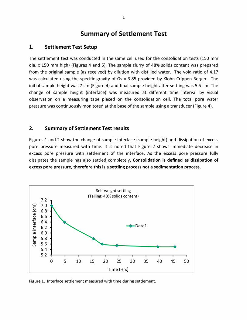
1. Settlement Test Setup
The settlement test was conducted in the same cell used for the consolidation tests (150 mm
dia. x 150 mm high) (Figures 4 and 5). The sample slurry of 48% solids content was prepared
from the original sample (as received) by dilution with distilled water. The void ratio of 4.17
was calculated using the specific gravity of Gs = 3.85 provided by Klohn Crippen Berger. The
initial sample height was 7 cm (Figure 4) and final sample height after settling was 5.5 cm. The
change of sample height (interface) was measured at different time interval by visual
observation on a measuring tape placed on the consolidation cell. The total pore water
pressure was continuously monitored at the base of the sample using a transducer (Figure 4).
2. Summary of Settlement Test results
Figures 1 and 2 show the change of sample interface (sample height) and dissipation of excess
pore pressure measured with time. It is noted that Figure 2 shows immediate decrease in
excess pore pressure with settlement of the interface. As the excess pore pressure fully
dissipates the sample has also settled completely. Consolidation is defined as dissipation of
excess pore pressure, therefore this is a settling process not a sedimentation process.
Figure 1. Interface settlement measured with time during settlement.
5.2
5.4
5.6
5.8
6.0
6.2
6.4
6.6
6.8
7.0
7.2
0 5 10 15 20 25 30 35 40 45 50
Data1
Time (Hrs)
Sa
mp
le in
terf
ace
(cm
)
Self-weight settling
(Tailing: 48% solids content)

2
Figure 2. Excess pore pressure dissipation during settlement.
0.00
0.05
0.10
0.15
0.20
0.25
0.30
0 5 10 15 20 25 30 35 40 45 50
Data2
Exc
ess
po
re p
ress
ure
(kP
a)
Time (Hrs)
Self-weight settling
Tailings: 48% solids content)

3
Figure 3. Settlement test conducted in a consolidation cell at the beginning of the test.
Figure 4. Settlement test conducted in a consolidation cell at the end of the test.
Transducer for
pore pressure
measurement
Tailings slurried sample