Attributing variation in a regional climate change

modelling experiment.

Christopher A. T. Ferro∗

April 28, 2004

Keywords: analysis of variance, climate change, regional modelling experiment

1 Introduction

This note demonstrates a simple analysis of variance for quantifying the uncertaintyarising from different components of the PRUDENCE experiments. This systematicexploration of experiment results helps to identify the relative importance of the differ-ent components, to construct simplifying syntheses of simulation output, and to makeinferences about climate change and model differences. The presented analysis quan-tifies the effects of different forcings, global models (GCMs), regional models (RCMs)and combinations of these factors. The methods used are introduced in Chapter 9 ofvon Storch and Zwiers (2001), who also cite more detailed references.

The example considers annual mean two-metre air temperatures from four climate-change experiments: the common control (CTL) and A2 scenario (SA2) runs of HIRHAM(DMI) and RCAO (SMHI) driven by both HadAM3H (HAD) and ECHAM4 (ECH).The annual means are computed from the monthly means interpolated onto the CRUgrid. The methods are first illustrated with the temperatures averaged over land pointsand then applied separately at each grid point to reveal the spatial structure.

2 Analysis of variance

2.1 Basic model

Let Yijkl be the annual mean two-metre air temperature averaged over land points forscenario i, GCM j, RCM k and year l. Each of the first three factors has two levels:

∗Address for correspondence: Department of Meteorology, University of Reading, Earley Gate,

P.O. Box 243, Reading, RG6 6BB, UK. E-mail: c.a.t.ferro@reading.ac.uk

1

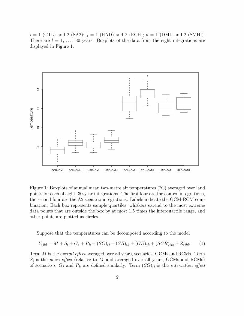
i = 1 (CTL) and 2 (SA2); j = 1 (HAD) and 2 (ECH); k = 1 (DMI) and 2 (SMHI).There are l = 1, . . . , 30 years. Boxplots of the data from the eight integrations aredisplayed in Figure 1.

ECH−DMI ECH−SMHI HAD−DMI HAD−SMHI ECH−DMI ECH−SMHI HAD−DMI HAD−SMHI

810

1214

Tem

pera

ture

Figure 1: Boxplots of annual mean two-metre air temperatures (◦C) averaged over landpoints for each of eight, 30-year integrations. The first four are the control integrations,the second four are the A2 scenario integrations. Labels indicate the GCM-RCM com-bination. Each box represents sample quartiles, whiskers extend to the most extremedata points that are outside the box by at most 1.5 times the interquartile range, andother points are plotted as circles.

Suppose that the temperatures can be decomposed according to the model

Yijkl = M + Si + Gj + Rk + (SG)ij + (SR)ik + (GR)jk + (SGR)ijk + Zijkl. (1)

Term M is the overall effect averaged over all years, scenarios, GCMs and RCMs. TermSi is the main effect (relative to M and averaged over all years, GCMs and RCMs)of scenario i; Gj and Rk are defined similarly. Term (SG)ij is the interaction effect

2

(relative to M +Si +Gj and averaged over all years and RCMs) of combining scenario iand GCM j; (SR)ik and (GR)jk are defined similarly. Term (SGR)ijk is the 3rd-order

interaction effect (relative to the sum of all previous effects and averaged over all years)of combining scenario i, GCM j and RCM k. The Zijkl are independent and identicallydistributed N(0, σ2) variables representing inter-annual variation. This basic modelassumes that within each integration the output (Yijk1, . . . , Yijk30) is a sequence ofindependent and identically distributed Normal random variables, the variances ofwhich are the same for all integrations. Extensions of this model are proposed inSection 3.

2.2 Parameter estimation

Estimators for the terms in model (1) are given in Table 1, where dot (·) subscripts de-note mean with respect to the corresponding indices, for example Yijk. =

∑

30

l=1Yijkl/30.

Effect EstimatorM Y....

Si Yi... − Y....

Gj Y.j.. − Y....

Rk Y..k. − Y....

(SG)ij Yij.. − Yi... − Y.j.. + Y....

(SR)ik Yi.k. − Yi... − Y..k. + Y....

(GR)jk Y.jk. − Y.j.. − Y..k. + Y....

(SGR)ijk Yijk. − Yij.. − Yi.k. − Y.jk. + Yi... + Y.j.. + Y..k. − Y....

Table 1: Estimators for the terms in model (1).

The variances of the estimators in Table 1 follow from the identity

var

(

∑

i

ciXi

)

=∑

i

c2

i var(Xi) +∑

i6=j

cicjcov(Xi, Xj)

for constants ci and random variables Xi, and the assumption that the Yijkl are inde-pendent, each with variance σ2. For example, the variance of the estimator for M isσ2/(IJKL), where I = 2, J = 2, K = 2 and L = 30 are the number of levels of thedifferent factors. Estimated variances are obtained by replacing the residual varianceσ2 with its estimator

σ̂2 =1

IJK(L − 1)

∑

ijkl

(Yijkl − Yijk.)2.

3

The estimators in Table 1 can be evaluated for the PRUDENCE data using theinformation in Table 2. The results are displayed in Table 3. By construction, summingany estimator over a single dimension yields zero (S1 + S2 = 0 for example) so, sincethe factors each have only two levels, it is sufficient to quote the effects estimated whenall subscripts are equal to 1. The residual variance is σ̂2 = 0.42.

HAD ECHDMI SMHI Mean DMI SMHI Mean DMI SMHI Mean

CTL 8.20 8.70 8.45 7.64 8.53 8.08 7.92 8.61 8.27SA2 12.08 12.53 12.31 12.59 13.53 13.06 12.34 13.03 12.68Mean 10.14 10.62 10.38 10.12 11.03 10.57 10.13 10.82 10.48

Table 2: Means of the annual mean two-metre air temperatures (◦C) averaged overland points split by scenario, GCM and RCM. The standard errors for means across0, 1, 2 and 3 factors are 0.12, 0.083, 0.059 and 0.042◦C.

M S1 G1 R1 (SG)11 (SR)11 (GR)11 (SGR)111

10.48 −2.21 −0.10 −0.35 0.28 −0.00 0.11 −0.01

Table 3: Estimated effects (◦C), each with standard error 0.042◦C.

2.3 Variance decomposition

The total sum of squares about the mean, which is a scaled version of the samplevariance, can be decomposed into contributions from the different terms in model (1):

∑

ijkl

(Yijkl − Y....)2 =

∑

ijkl

S2

i +∑

ijkl

G2

j +∑

ijkl

R2

k +∑

ijkl

(SG)2

ij +∑

ijkl

(SR)2

ik

+∑

ijkl

(GR)2

jk +∑

ijkl

(SGR)2

ijk +∑

ijkl

(Yijkl − Yijk.)2. (2)

The final term in the decomposition is called the residual sum of squares. Thecontributions are listed in Table 4, often called an ‘analysis of variance’ table, andexpressed as a proportion of the total sum of squares. The model explains 92.7% of thevariation in the data, with 7.3% attributed to residual (inter-annual) variation. Theinterpretation of the other components is deferred to Section 2.5.

4

SS % DF MS F pS 1170.21 88.7 1 1170.21 2817.81 0.000G 2.21 0.2 1 2.21 5.33 0.022R 28.81 2.2 1 28.81 69.38 0.000SG 18.73 1.4 1 18.73 45.10 0.000SR 0.00 0.0 1 0.00 0.00 0.994GR 2.84 0.2 1 2.84 6.83 0.010SGR 0.03 0.0 1 0.03 0.08 0.779Residual 96.35 7.3 232 0.42Total 1319.19 100.0

Table 4: Analysis of variance table.

2.4 Model simplification

The statistical significance of terms in model (1) can be assessed with suitable tests.If terms are found to be insignificant then they can be removed, yielding a more par-simonious model, a simpler interpretation, and more precise estimates of quantities ofinterest.

The number of independent terms in the model associated with each of the sumsof squares (SS) in Table 4 is known as the degrees of freedom (DF). The mean squares

(MS) are the ratios SS/DF. The residual MS is the estimated residual variance σ̂2.Under the hypothesis that all levels of a particular factor are equal (S1 = S2 for

example) and by construction therefore zero, the ratio of the corresponding MS (withτ degrees of freedom) to σ̂2 (with ν degrees of freedom) has an Fτ,ν distribution.The p-value for the hypothesis test is the mass of the Fτ,ν distribution lying above theobserved value of the ratio. These test statistics and p-values are also shown in Table 4.The data from the eight integrations are balanced, which means that there is an equalnumber (L = 30) of replications for each of the eight possible combinations of levels ofthe three factors. If this were not the case then Table 4 would need modifying beforeconducting the hypothesis tests.

Both the terms SGR and SR have large p-values. Ignoring these terms leaves amodel in which the expectations of climate-change responses, Y2jk. − Y1jk., are inde-pendent of the RCM, k. Interaction remains, however, between scenario and GCM,and between RCM and GCM. Consequently, the estimated effects in Table 3 must beinterpreted carefully. For example, the GCM term G has a small p-value and encour-ages the conclusion that the GCM effects are different from each other, with ECHAM4warmer than HadAM3H by about G2−G1 = 0.10− (−0.10) = 0.20◦C. This conclusionis incorrect, however, as will be shown below. The confusion arises because the GCMeffects G1 and G2 average over all possible scenario and RCM combinations, whereas

5

the presence of SG and GR interactions necessitates the inspection of the GCM effectsfor each combination separately.

2.5 Contrasts

The model can be used to make inferences about linear combinations of terms in themodel that may be more interesting than the original effects. For notational conve-nience, denote the expectation of Yijk. by µijk. A contrast is a linear combination∑

ijk cijkµijk in which the coefficients sum to zero:∑

ijk cijk = 0. Two contrasts,∑

ijk cijkµijk and∑

ijk c′ijkµijk are orthogonal if∑

ijk cijkc′ijk = 0. The greatest possible

number of mutually orthogonal contrasts is IJK − 1.The estimator for a contrast is c =

∑

ijk cijkYijk. with estimated variance s2 =

σ̂2∑

ijk c2

ijk/L. A 100(1 − α)%-confidence interval is c ± tν(1 − α/2)s, where tν(α) isthe α-quantile of the t distribution with ν = IJK(L−1) degrees of freedom. The sum ofsquares associated with a contrast is SS = L(

∑

ijk cijkYijk.)2/∑

ijk c2

ijk with one degree

of freedom, and the statistical significance can be quantified by comparing MS/σ̂2 withthe F1,ν distribution. The sums of squares from a set of IJK − 1 orthogonal contraststotal the model sum of squares

∑

ijkl(Yijk. − Y....)2, which is the difference between the

total and residual sums of squares.When there are only two levels of each factor, the sums of squares in decomposi-

tion (2) correspond to sums of squares for a set of easily interpretable orthogonal con-trasts. For example, the contrast S2 − S1 = µ2.. − µ1.. has coefficients cijk = (−JK)−i

and sum of squaresL(S2 − S1)

2

I/(JK)= JKL

∑

i

S2

i =∑

ijkl

S2

i

since S2 = −S1. The seven orthogonal contrasts are described in Table 5. The first isthe mean climate-change response. The others are the differences between the

• GCM main effects,

• RCM main effects,

• mean climate-change responses of the GCMs,

• mean climate-change responses of the RCMs,

• mean effects of the GCMs on the RCMs,

• mean effects of the GCMs on the climate-change responses of the RCMs.

These contrasts help to interpret the information in Table 4. The climate-changeresponse explains 88.7% of the variation in the data and this difference between the sce-nario main effects is highly statistically significant (p = 0.000). Inter-annual variability

6

Term ContrastS µ2.. − µ1..

G µ.2. − µ.1.

R µ..2 − µ..1

SG ∆µ2. − ∆µ1.

SR ∆µ.2 − ∆µ.1

GR (µ.22 − µ.12) − (µ.21 − µ.11)SGR (∆µ22 − ∆µ12) − (∆µ21 − ∆µ11)

Table 5: The set of orthogonal contrasts corresponding to decomposition (2). Define∆µjk = µ2jk − µ1jk to be the mean climate-change response for GCM j and RCM k.

explains the next largest proportion (7.3%) of the variation. Although the differencesbetween the GCM main effects and between the RCM main effects explain only 0.2%and 2.2% of the variation, and so might be considered practically insignificant, theyare both statistically significant at the 5% level. The amount of variation accountedfor by the difference between the mean climate-change responses of the GCMs (1.4%)is greater than that accounted for by the difference between the mean climate-changeresponses of the RCMs (0.0%), the latter being statistically insignificant (p = 0.994).The difference between the effects of the GCMs on the RCMs accounts for just 0.2%of the variation but is statistically significant at the 1% level. In contrast, the differ-ence between the effects of the GCMs on the climate-change responses of the RCMs isstatistically insignificant (p = 0.779).

More detailed constrasts can now be considered. The similarity of the meanclimate-change responses of the RCMs noted earlier suggests that the following (non-orthogonal) contrasts are sufficient to quantify all of the statistically significant differ-ences.

1. The difference between scenarios (climate-change response) for each GCM, aver-aging over RCM:

(a) HAD (µ21. − µ11.)

(b) ECH (µ22. − µ12.)

2. The difference between RCMs for each GCM, averaging over scenario:

(a) HAD (µ.12 − µ.11)

(b) ECH (µ.22 − µ.21)

3. The difference between GCMs for each scenario-RCM combination:

7

(a) CTL-DMI (µ121 − µ111)

(b) CTL-SMHI (µ122 − µ112)

(c) SA2-DMI (µ221 − µ211)

(d) SA2-SMHI (µ222 − µ212)

Confidence intervals and p-values for these contrasts are given in Table 6. Thefollowing conclusions can be drawn. The A2 scenario is warmer than the controlscenario for both GCMs; RCAO is warmer than HIRHAM for both GCMs; ECHAM4is warmer than HadAM3H for both RCMs in the A2 scenario, but in the control scenarioHadAM3H is warmer than ECHAM4 for HIRHAM, and there is little difference forRCAO. These relationships are evident in Figure 1.

Contrast Estimate CI SS F p1a µ21. − µ11. 3.86 (3.63, 4.09) 446.42 1074.97 0.0001b µ22. − µ12. 4.97 (4.74, 5.21) 742.52 1787.95 0.0002a µ.12 − µ.11 0.72 (0.48, 0.95) 15.39 37.07 0.0002b µ.22 − µ.21 0.91 (0.68, 1.14) 24.87 59.88 0.0003a µ121 − µ111 −0.56 (−0.89,−0.23) 4.72 11.36 0.0013b µ122 − µ112 −0.17 (−0.50, 0.16) 0.45 1.08 0.3013c µ221 − µ211 0.51 (0.18, 0.84) 3.90 9.40 0.0023d µ222 − µ212 0.99 (0.66, 1.32) 14.75 35.51 0.000

Table 6: Estimated contrasts, 95% confidence intervals (CI) and p-values.

The contrasts in Table 6 were considered only after, and indeed motivated by, theinitial analysis of the data. When such a set of ‘unplanned’ contrasts is tested, thesignificance levels of the tests or, equivalently, the coverages of the confidence intervalsshould be adjusted to account for the likelihood of obtaining an erroneously significantdifference by chance. This multiple comparisons problem has not been addressed here,but the literature describes many possible adjustments. See Milliken and Johnson(1984) for example.

2.6 Grid-point analysis

Model (1) was estimated at each point on the CRU grid. Figure 2 shows the proportionof variation explained by the different components of the model. These plots providea summary of the sources of variation in the modelling experiment. The followingconclusions can be drawn.

8

• The proportion of variance explained by the model is at least 75% everywhere, isgreater over water and increases from north-east to south-west. The inter-annualvariation is around 10% over land and around 5% over water.

• The proportion of variation explained by the differences in scenario main effectsincreases from 30% in the north-west to near 100% in the south-east, with lowervalues in mountainous regions and in the Baltic Sea.

• Most of the remaining variation in the Atlantic is explained by the differencesbetween the GCM main effects, with smaller contributions from the differencesin GCM climate-change responses and in RCM main effects.

• Almost all of the remaining variation in the Baltic Sea is explained by the GCMmain effect.

• Some of the remaining variation over land, the Mediterranean and North Seas isexplained by the GCM response, but in mountainous regions, Scandinavia andaround the Adriatic Sea a greater part is explained by the RCM main effect.

Figure 3 identifies those interaction effects in the model that are significant at the5% level. The following conclusions can be drawn.

• The third-order interaction is significant only in the North Atlantic (grey).

• All three second-order terms are significant in central Europe (white).

• In the rest of Europe, the scenario-RCM interaction is significant only in the farnorth (green).

• The GCM-RCM interaction is insignificant over the rest of Northern Europe, theAlps and the Mediterranean Sea (yellow).

• The scenario-GCM interaction is insignificant over the Baltic Sea and Turkey(red).

Estimated contrasts comparing the two levels of each factor for all combinations oflevels of the other factors are shown in Figures 4–6. The following conclusions can bedrawn.

• The A2 scenario is everywhere warmer than the control for all GCM-RCM com-binations, and the difference typically increases from north-west to south-eastand with distance from the coast.

9

• ECHAM4 is cooler than HadAM3H around the Baltic Sea for all scenario-RCMcombinations; in the control, ECHAM4 is also cooler in central and eastern Eu-rope for HIRHAM; in the scenario, ECHAM4 is warmer in Scandinavia, western,central and southern Europe.

• RCAO is cooler than HIRHAM over water and warmer over land, particularly inmountainous regions, for all scenario-GCM combinations.

Estimated contrasts comparing the climate-change responses (SA2 − CTL) of thetwo GCMs for each RCM and of the two RCMs for each GCM are shown in Figure 7.The following conclusions can be drawn.

• The ECHAM4 response is generally greater than the HadAM3H response, par-ticularly in the west and over land.

• The reponse of HIRHAM is everywhere similar to that of RCAO for HadAM3H,but for ECHAM4 is greater in the north, and lower north of the Alps and westof the Pyrenees.

The final bullet point highlights another potential benefit of performing an analysisof variance. If the main feature of interest were the mean climate-change response withHadAM3H boundary conditions then the analysis suggests that it would be sufficientto plot a map of the response averaged across both RCMs rather than separate mapsfor RCAO and HIRHAM. Note, however, that this conclusion might change if a morecareful analysis, using techniques described in the following section, were conducted.

10

Figure 2: Percentage of variation explained by a) the full model, b) the differences in thescenarios (S), c) the inter-annual variation, and by the differences in d) the GCMs (G),e) the RCMs (R), f) the GCM-RCM interaction (GR), g) the GCM responses (SG),h) the RCM responses (SR), and i) the GCM-RCM response interaction (SGR).

11

Figure 3: The interactions that are significant at the 5% level. Lower order terms areconsidered significant if corresponding higher order terms are significant.

12

Figure 4: Contrasts (◦C) between scenarios (SA2 − CTL) for four GCM-RCM combi-nations: a) HAD-DMI, b) HAD-SMHI, c) ECH-DMI and d) ECH-SMHI. Grid pointsat which the contrast is insignificant at the 1% level are masked.

13

Figure 5: Contrasts (◦C) between GCMs (ECH − HAD) for four scenario-RCM com-binations: a) CTL-DMI, b) CTL-SMHI, c) SA2-DMI and d) SA2-SMHI. Grid pointsat which the contrast is insignificant at the 1% level are masked.

14

Figure 6: Contrasts (◦C) between RCMs (SMHI − DMI) for four scenario-GCM com-binations: a) CTL-HAD, b) CTL-ECH, c) SA2-HAD and d) SA2-ECH. Grid points atwhich the contrast is insignificant at the 1% level are masked.

15

Figure 7: Response (SA2− CTL) contrasts (◦C) between GCMs (ECH −HAD) for a)DMI and b) SMHI, and between RCMs (SMHI−DMI) for c) HAD and d) ECH. Gridpoints at which the contrast is insignificant at the 1% level are masked.

16

3 Extending the model

This section proposes some extensions to model (1) that represent the data more ac-curately and support more detailed inferences. The deficiencies of the basic model forthe land-averaged data are illustrated with diagnostic plots.

3.1 Diagnostics

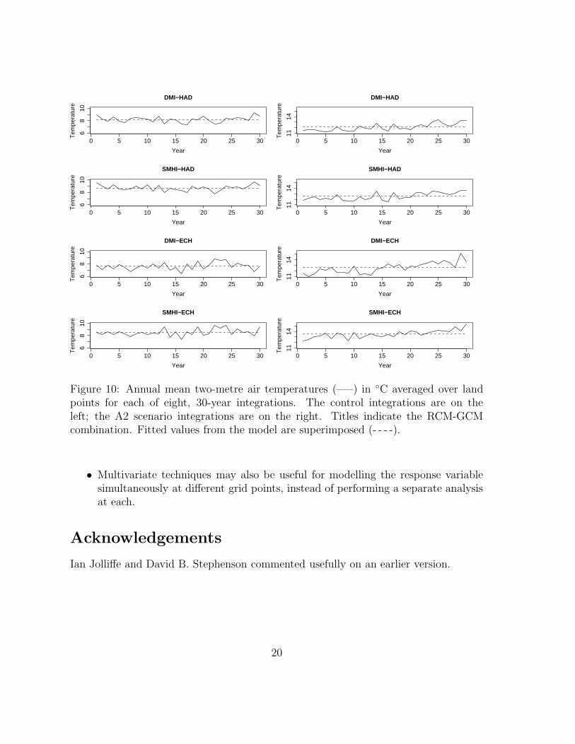
The quantile-quantile plots in Figure 8 indicate that the assumption of normally dis-tributed residuals is poor: the residuals have lighter tails in the control runs, and arelatively flat distribution in the scenario runs. Some outliers are also evident. Theassumption of common variance is also unacceptable: the boxplots in Figure 9 indicatethat there is greater variation in the scenario runs. The model fit is assessed in Fig-ure 10 and is inadequate: trends in the scenario runs are overlooked, which is reflectedin positive serial correlation (not shown) in the corresponding residuals.

The model assumptions are untenable. Features of the data are not captured by themodel and previous inferences may be inaccurate. More elaborate models and inferenceprocedures that avoid these shortcomings are discussed in the following sections.

3.2 Model structure

• Trends could be accounted for by including covariates in the model:

Yijkl = M + . . . + (SGR)ijk + βijkxijkl + Zijkl

for example, where xijkl could be a measure of time, the HadCM3 boundaryconditions, or the scenario emissions forcings. Another approach (Sexton et al.,2003) that includes an extra factor with one level for each time period could alsobe used, but requires additional observations if the full model is to be estimated.

• More levels of the scenario, GCM and RCM factors could be added, althoughthe data are then likely to be unbalanced and inference becomes more compli-cated. Different ensemble members could also be added, and considered either asindependent replicates or as another factor representing intra-ensemble variation.

• Repeated measures models (for example Milliken and Johnson, 1984) that explic-itly recognise the time ordering of the data can also be employed.

3.3 Error distribution

• Inference becomes complicated if the residuals are not normally distributed. How-ever, it might be hoped that a satisfactory model would achieve approximatelynormal residuals.

17

D

DD

D

DD

DD

DD

D

D

D

DD

DD

DD

D

D

DD

DD

DD

D

D

D

S

S

S

S

SSS

S

S

S

S

S

S

SS

SS

S

S

S

S

S

S

SS

SS

S

S

Sd

d

d

d

d

d

d

d

d

d

d

d

d

d

d

d

d

d

d

d

d

dd

d

d

d

dd

d

ds

s

s

s

s

s

s

ss

ss

s

s

s

s

s

s

s

s

ss

s

s

s

s

s

ss

s

s

−4 −2 0 2 4

−4

−2

02

4

Normal Quantiles

Sta

ndar

dise

d R

esid

uals

DDDDDD

D

DDD

D

DD

D

D

D

D

DD

D

DD

D

D

D

DD

D

DD

S

SS

SS

S

S

SSS

S

SS

S

SS

S

SSS

SS

S

SS

SS

S

SS

d

d

d

dd

d

ddd

d

dd

d

dd

d

d

d

d

dd

dd

d

d

d

d

d

d

d

ss

ss

s

s

ss

s

s

s

s

s

ss

s

s

s

s

ss

s

s

ss

ss

s

s

s

−4 −2 0 2 4

−4

−2

02

4

Normal Quantiles

Sta

ndar

dise

d R

esid

uals

Figure 8: Plots of standardised residuals against standard normal quantiles for thecontrol (left) and scenario (right) integrations. Labels indicate the RCM-GCM combi-nation: DMI-HAD (D), DMI-ECH (d), SMHI-HAD (S) and SMHI-ECH (s).

• Statistical tests for unequal variances are available. If equality of variances isrejected then inference procedures can be adapted. Results are typically robustto unequal variances, however, as long as the data are approximately balanced(Milliken and Johnson, 1984, page 17).

• Even after modelling trends, the residuals might be serially dependent. Modellingthis dependence, replacing Zijkl with an auto-regressive process for example, leadsto a general linear (time-series) model, for which inference is more complicated.

3.4 Random effects

• All of the models proposed thus far have been fixed effect models, that is the termsin the model are assumed to be unknown constants. This is natural if interest

18

ECH−DMI ECH−SMHI HAD−DMI HAD−SMHI ECH−DMI ECH−SMHI HAD−DMI HAD−SMHI

−1

01

2

Res

idua

ls

Figure 9: Boxplots of residuals (◦C) for each of eight, 30-year integrations. The firstfour are the control integrations; the second four are A2 scenario integrations. Labelsindicate the GCM-RCM combination.

is in those particular levels of the different factors: those particular RCMs forexample. For statements about climate change, however, it may be more naturalto treat the GCM and RCM effects as random, to assume that they are a sampleof all possible GCMs and RCMs, and to make inferences about these GCM andRCM populations and their effects. Models in which all terms are random areknown as random effect models; models with both fixed and random effects areknown as mixed effect models. See von Storch and Zwiers (2001) for details.

3.5 Multivariate models

• Instead of using only two-metre air temperatures for the response variable Y ,multivariate techniques could be used to model several variables simultaneously.

19

0 5 10 15 20 25 30

68

10

Year

Tem

pera

ture

DMI−HAD

0 5 10 15 20 25 30

1114

Year

Tem

pera

ture

DMI−HAD

0 5 10 15 20 25 30

68

10

Year

Tem

pera

ture

SMHI−HAD

0 5 10 15 20 25 30

1114

Year

Tem

pera

ture

SMHI−HAD

0 5 10 15 20 25 30

68

10

Year

Tem

pera

ture

DMI−ECH

0 5 10 15 20 25 3011

14Year

Tem

pera

ture

DMI−ECH

0 5 10 15 20 25 30

68

10

Year

Tem

pera

ture

SMHI−ECH

0 5 10 15 20 25 30

1114

Year

Tem

pera

ture

SMHI−ECH

Figure 10: Annual mean two-metre air temperatures (—–) in ◦C averaged over landpoints for each of eight, 30-year integrations. The control integrations are on theleft; the A2 scenario integrations are on the right. Titles indicate the RCM-GCMcombination. Fitted values from the model are superimposed (- - - -).

• Multivariate techniques may also be useful for modelling the response variablesimultaneously at different grid points, instead of performing a separate analysisat each.

Acknowledgements

Ian Jolliffe and David B. Stephenson commented usefully on an earlier version.

20

References

Milliken GA and Johnson DE (1984) Analysis of Messy Data Volume I: Designed

Experiments. Wadsworth.

Sexton DMH, Grubb H, Shine KP and Folland CK (2003) Design and analysis ofclimate model experiments for the efficient estimation of anthropogenic signals.Journal of Climate, 16, 1320–1336.

von Storch H and Zwiers FW (2001) Statistical Analysis in Climate Research. Cam-bridge University Press.

21