Audun Jøsang. Conditional Reasoning with Subjective Logic.

This article is published in Journal of Multiple-Valued Logic and Soft Computing 2008, 15(1), 5-38.

Published in DUO with permission from Old City Publishing.

Conditional Reasoning with Subjective Logic⋆

AUDUN JØSANG

University of OsloUNIK Graduate Center

NorwayEmail: josang @ unik.no

Conditional inference plays a central role in logical and Bayesianreasoning, and is used in a wide range of applications. It ba-sically consists of expressing conditional relationship betweenparent and child propositions, and then to combine those con-ditionals with evidence about the parent propositions in order toinfer conclusions about the child propositions. While conditionalreasoning is a well established part of classical binary logic andprobability calculus, its extension to belief theory has only re-cently been proposed. Subjective opinions represent a specialtype of general belief functions. This article focuses on condi-tional reasoning in subjective logic where beliefs are representedin the form of binomial or multinomial subjective opinions.Bi-nomial conditional reasoning operators for subjective logic havebeen defined in previous contributions. We extend this approachto multinomial opinions, thereby making it possible to representconditional and evidence opinions on frames of arbitrary size.This makes subjective logic a powerful tool for conditionalrea-soning in situations involving ignorance and partial information,and makes it possible to analyse Bayesian network models withuncertain probabilities.

Key words:Subjective logic, Conditional, Deduction, Abduction, Belieftheory, Bayesian networks

⋆ Preprint of article published in theJournal of Multiple-Valued Logic and Soft Computing15(1), pp.5-38, Old City Publishing, 2008.

1

1 INTRODUCTION

Conditionals are propositions like“If we don’t hurry we’ll be late for theshow” or “If it rains, Michael will carry an umbrella” which are of the form“IF x THEN y” wherex denotes the antecedent andy the consequent propo-sition. The truth value of conditionals can be evaluated in different ways, e.g.as binary TRUE or FALSE, as a probability measure or as an opinion. Con-ditionals are complex propositions because they contain anantecedent and aconsequent that are also propositions with truth values that can be evaluatedin the same way. Conditionals can be linked e.g. by letting a conditionalproposition be the antecedent of another conditional proposition.

The idea of having a conditional connection between an antecedent and aconsequent proposition can be traced back to Ramsey [21] whoarticulatedwhat has become known as Ramsey’s Test:To decide whether you believe aconditional, provisionally or hypothetically add the antecedent to your stockof beliefs, and consider whether to believe the consequent. This idea wastranslated into a formal language by Stalnaker [27] in the form of the so-calledStalnaker’s Hypothesis, formally expressed as:p(IF x THEN y) = p(y|x).The interpretation of Stalnaker’s Hypothesis is that the probability of the con-ditional proposition “IFx THEN y” is equal to the probability of the propo-sition y given that the propositionx is TRUE. A more precise expression ofStalnaker’s hypothesis is thereforep(IF x THEN y) = p(y|(p(x) = 1)), butthe bulkiness of this notation would make it impractical.

An alternative viewpoint to that of Stalnaker was put forward by Lewis[18] who argued that conditional propositions do not have truth-values andthat they do not express propositions. This would mean that for any propo-sitionsx andy, there is no propositionz for which p(z) = p(y|x), so theconditional probability can not be the same as the probability of conditionals.

In our opinion Stalnaker’s Hypothesis is sound and applicable for condi-tional reasoning. We would argue against Lewis’ view by simply saying thatit is meaningful to assign a probability to a conditional proposition like “y|x”,which is defined in casex is true, and undefined in casex is false.

Meaningful conditional deduction requires relevance between antecedentand consequent, i.e. that the consequent depends on the antecedent. Condi-tionals that are based on the dependence between consequentand antecedentare universally valid, and are calledlogical conditionals[3]. Deduction withlogical conditionals reflect human intuitive conditional reasoning.

Both binary logic and probability calculus have mechanismsfor condi-tional reasoning. In binary logic, Modus Ponens (MP) and Modus Tollens

2

(MT) are the classical operators which are used in any field oflogic that re-quires conditional deduction. In probability calculus, binomial conditionaldeduction is expressed as:

p(y‖x) = p(x)p(y|x) + p(x)p(y|x) (1)

where the terms are interpreted as follows:

p(y|x) : the conditional probability ofy givenx is TRUEp(y|x) : the conditional probability ofy givenx is FALSEp(x) : the probability of the antecedentx

p(x) : the probability of the antecedent’s complement (= 1 − p(x))p(y‖x) : the deduced probability of the consequenty

The notationy‖x, introduced in [15], denotes that the truth or probabilityof propositiony is deduced as a function of the probability of the antecedentx together with the conditionals. The expressionp(y‖x) thus represents aderived value, whereas the expressionsp(y|x) andp(y|x) represent input val-ues together withp(x). Below, this notational convention will also be usedfor opinions in subjective logic.

This article describes how the same principles for conditional inferenceoutlined above can be formulated in subjective logic. The advantage of thisapproach is that conditional reasoning models can be analysed with subjectiveopinions as input and output values, i.e. in the presence of uncertainty andpartial ignorance. This will also allow the analyst to appreciate the relativeproportions of firm evidence and uncertainty as contributing factors to thederived probabilistic likelihoods.

This article is structured as follows. Section 2 reviews probabilistic con-ditional reasoning in order to provide a benchmark for subjective logic de-scribed later. Section 3 reviews the belief representationused in classicalDempster-Shafer belief theory as a background for subjective opinions. Sec-tion 4 provides a brief review of previous approaches to conditional beliefreasoning. Section 5 describes subjective opinions which are used as argu-ments in subjective logic. Section 6 describes conditionaldeduction and ab-duction in subjective logic, and Section 7 describes how Bayesian networkscan be based on subjective logic. Section 8 suggests application domains ofconditional reasoning with subjective logic, and concludes the presentation.

3

2 PROBABILISTIC CONDITIONAL REASONING

Classical results from probabilistic conditional reasoning are briefly reviewedbelow in order to provide a benchmark for conditional reasoning with subjec-tive logic, described in Sec.6.

2.1 Binomial Conditional ReasoningProbabilistic conditional reasoning is used extensively in areas where conclu-sions need to be derived from probabilistic input evidence,such as for makingdiagnoses from medical tests. A pharmaceutical company that develops a testfor a particular infection disease will typically determine the reliability of thetest by letting a group of infected and a group of non-infected people undergothe test. The result of these trials will then determine the reliability of thetest in terms of itssensitivityp(x|y) andfalse positive ratep(x|y), wherex:“Positive Test”, y: “Infected” andy: “Not infected”. The conditionals areinterpreted as:

• p(x|y): “The probability of positive test given infection”

• p(x|y): “The probability of positive test in the absence of infection” .

The problem with applying these reliability measures in a practical settingis that the conditionals are expressed in the opposite direction to what thepractitioner needs in order to apply the expression of Eq.(1). The conditionalsneeded for making the diagnosis are:

• p(y|x): “The probability of infection given positive test”

• p(y|x): “The probability of infection given negative test”

but these are usually not directly available to the medical practitioner. How-ever, they can be obtained if the base rate of the infection isknown.

The base rate fallacy [17] in medicine consists of making theerroneous as-sumption thatp(y|x) = p(x|y). While this reasoning error often can producea relatively good approximation of the correct diagnostic probability value, itcan lead to a completely wrong result and wrong diagnosis in case the baserate of the disease in the population is very low and the reliability of the testis not perfect. The required conditionals can be correctly derived by invert-ing the available conditionals using Bayes rule. The inverted conditionals areobtained as follows:

p(x|y) = p(x∧y)p(y)

p(y|x) = p(x∧y)p(x)

⇒ p(y|x) =p(y)p(x|y)

p(x). (2)

4

On the right hand side of Eq.(2) the base rate of the disease inthe populationis expressed byp(y). By applying Eq.(1) withx andy swapped in everyterm, the expected rate of positive testsp(x) in Eq.(2) can be computed as afunction of the base ratep(y). In the following,a(x) anda(y) will denote thebase rates ofx andy respectively. The required conditional is:

p(y|x) =a(y)p(x|y)

a(y)p(x|y) + a(y)p(x|y). (3)

A medical test result is typically considered positive or negative, so whenapplying Eq.(1) it can be assumed that eitherp(x) = 1 (positive) orp(x)

= 1 (negative). In case the patient tests positive, Eq.(1) can be simplified top(y‖x) = p(y|x) so that Eq.(3) will give the correct likelihood that the patientactually has contracted the disease.

2.2 Example 1: Probabilistic Medical ReasoningLet the sensitivity of a medical test be expressed asp(x|y) = 0.9999 (i.e.an infected person will test positive in 99.99% of the cases)and the falsepositive rate bep(x|y) = 0.001 (i.e. a non-infected person will test posi-tive in 0.1% of the cases). Let the base rate of infection in populationA be1% (expressed asa(yA)=0.01) and let the base rate of infection in popula-tion B be 0.01% (expressed asa(yB)=0.0001). Assume that a person frompopulationA tests positive, then Eq.(3) and Eq.(1) lead to the conclusion thatp(yA‖x) = p(yA|x) = 0.9099 which indicates a 91% likelihood that the per-son is infected. Assume that a person from populationB tests positive, thenp(yB‖x) = p(yB|x) = 0.0909 which indicates only a 9% likelihood that theperson is infected. By applying the correct method the base rate fallacy isavoided in this example.

2.3 Deductive and Abductive ReasoningIn the general case where the truth of the antecedent is expressed as a proba-bility, and not just binary TRUE and FALSE, the opposite conditional is alsoneeded as specified in Eq.(1). In case the negative conditional is not directlyavailable, it can be derived according to Eq.(3) by swappingx andx in everyterm. This produces:

p(y|x) = a(y)p(x|y)a(y)p(x|y)+a(y)p(x|y)

= a(y)(1−p(x|y))a(y)(1−p(x|y))+a(y)(1−p(x|y)) .

(4)

Eq.(3) and Eq.(4) enables conditional reasoning even when the requiredconditionals are expressed in the reverse direction to whatis needed.

5

The termframe⋆ will be used with the meaning of a traditional state spaceof mutually disjoint states. We will use the term“parent frame” and“childframe” to denote the reasoning direction, meaning that the parent frame iswhat the analyst has evidence about, and probabilities overthe child frame iswhat the analyst needs. Defining parent and child frames is thus equivalentwith defining the direction of the reasoning.

Forward conditional inference, calleddeduction, is when the parent frameis the antecedent and the child frame is the consequent of theavailable con-ditionals. Reverse conditional inference, calledabduction, is when the parentframe is the consequent, and the child frame is the antecedent.

Deductive and abductive reasoning situations are illustrated in Fig.1 wherex denotes a state in the parent frame andy denotes a state in the child frame.Conditionals are expressed asp(consequent|antecedent).

FIGURE 1Visualising deduction and abduction

The concepts of“causal” and“derivative” reasoning can be meaningfulfor clearly causal conditional relationships. By assumingthat the antecedentcauses the consequent, then causal reasoning is equivalentto deductive rea-soning, and derivative reasoning is equivalent to abductive reasoning.

In medical reasoning for example, the infection causes the test to be posi-tive, not the other way. The reliability of medical tests is expressed as causalconditionals, whereas the practitioner needs to apply the derivative invertedconditionals. Starting from a positive test to conclude that the patient is in-fected therefore represents derivative reasoning. Most people have a tendencyto reason in a causal manner even in situations where derivative reasoning is

⋆ Usually calledframe of discernmentin traditional belief theory

6

required. In other words, derivative situations are often confused with causalsituations, which provides an explanation for the tendencyof the base ratefallacy in medical diagnostics. In legal reasoning, the same type of reasoningerror is calledthe prosecutor’s fallacy.

2.4 Multinomial Conditional ReasoningSo far in this presentation the parent and child frames have consisted of binarysets{x, x} and {y, y}. In general, both the parent and child frames in aconditional reasoning situation can consist of an arbitrary number of disjointstates. LetX = {xi|i = 1 . . . k} be the parent frame with cardinalityk, andlet Y = {yj|j = 1 . . . l} be the child frame with cardinalityl. The deductiveconditional relationship betweenX andY is then expressed withk vectorconditionalsp(Y |xi), each being ofl dimensions. This is illustrated in Fig.2.

FIGURE 2Multinomial deductive vector conditionals between parentX and childY

The vector conditional~p(Y |xi) relates each statexi to the frameY . Theelements of~p(Y |xi) are the scalar conditionals expressed as:

p(yj |xi), wherel∑

j=1

p(yj |xi) = 1 . (5)

The probabilistic expression for multinomial conditionaldeduction fromX to Y , generalising that of Eq.(1), is the vectorp(Y ‖X) overY where eachscalar vector elementp(yj‖X) is:

p(yj‖X) =

k∑

i=1

p(xi)p(yj |xi) . (6)

7

The multinomial probabilistic expression for inverting conditionals, gen-eralising that of Eq.(3), becomes:

p(yj |xi) =a(yj)p(xi|yj)∑l

t=1 a(yt)p(xi|yt)(7)

wherea(yj) represents the base rate ofyj .By substituting the conditionals of Eq.(6) with inverted multinomial condi-

tionals from Eq.(7), the general expression for probabilistic abduction emerges:

p(yj‖X) =

k∑

i=1

p(xi)

(a(yj)p(xi|yj)∑l

t=1 a(yt)p(xi|yt)

). (8)

This will be illustrated by a numerical example below.

2.5 Example 2: Probabilistic Intelligence Analysis

Two countriesA andB are in conflict, and intelligence analysts of countryB

want to find out whether countryA intends to use military aggression. Theanalysts of countryB consider the following possible alternatives regardingcountryA’s plans:

y1 : No military aggression from countryAy2 : Minor military operations by countryAy3 : Full invasion of countryB by countryA

(9)

The way the analysts will determine the most likely plan of countryA is bytrying to observe movement of troops in countryA. For this, they have spiesplaced inside countryA. The analysts of countryB consider the followingpossible movements of troops.

x1 : No movement of countryA’s troopsx2 : Minor movements of countryA’s troopsx3 : Full mobilisation of all countryA’s troops

(10)

The analysts have defined a set of conditional probabilitiesof troop move-ments as a function of military plans, as specified by Table 1.

The rationale behind the conditionals are as follows. In case countryAhas no plans of military aggression(y1), then there is little logistic reasonfor troop movements. However, even without plans of military aggressionagainst countryB it is possible that countryA expects military aggressionfrom countryB, forcing troop movements by countryA. In case countryA

8

Troop movementsProbability x1 x2 x3

vectors No movemt. Minor movemt. Full mob.~p(X |y1): p(x1|y1) = 0.50 p(x2|y1) = 0.25 p(x3|y1) = 0.25

~p(X |y2): p(x1|y2) = 0.00 p(x2|y2) = 0.50 p(x3|y2) = 0.50

~p(X |y3): p(x1|y3) = 0.00 p(x2|y3) = 0.25 p(x3|y3) = 0.75

TABLE 1Conditional probabilitiesp(X|Y ): troop movementxi given military planyj

prepares for minor military operations against countryB (y2), then necessar-ily troop movements are required. In case countryA prepares for full invasionof countryB (y3), then significant troop movements are required.

Based on observations by spies of countryB, the analysts determine thelikelihoods of actual troop movements to be:

p(x1) = 0.00 , p(x2) = 0.50 , p(x3) = 0.50 . (11)

The analysts are faced with an abductive reasoning situation and must firstderive the conditionalsp(Y |X). The base rate of military plans is set to:

a(y1) = 0.70 , a(y2) = 0.20 , a(y3) = 0.10 . (12)

The expression of Eq.(7) can now be used to derive the required condition-als, which are given in Table 2 below.

Probabilities of military plans given troop movement~p(Y |x1) ~p(Y |x2) ~p(Y |x3)

Military plan No movemt. Minor movemt. Full mob.y1: No aggr. p(y1|x1) = 1.00 p(y1|x2) = 0.58 p(y1|x3) = 0.50

y2: Minor ops. p(y2|x1) = 0.00 p(y2|x2) = 0.34 p(y2|x3) = 0.29

y3: Invasion p(y3|x1) = 0.00 p(y3|x2) = 0.08 p(y3|x3) = 0.21

TABLE 2Conditional probabilitiesp(Y |X): military planyj given troop movementxi

The expression of Eq.(6) can then be used to derive the probabilities of

9

military plans of countryA, resulting in:

p(y1‖X) = 0.54 , p(y2‖X) = 0.31 , p(y3‖X) = 0.15 . (13)

Based on the results of Eq.(13), it seems most likely that country A doesnot plan any military aggression against countryB. Analysing the same ex-ample with subjective logic in Sec.6.4 will show that these results give amisleading estimate of countryA’s plans because they hide the underlyinguncertainty.

3 BELIEF REPRESENTATIONS

Traditional probabilities are not suitable for expressingignorance about thelikelihoods of possible states or outcomes. If somebody wants to expressignorance as“I don’t know” this would be impossible with a simple scalarprobability value. A probability 0.5 would for example meanthat the eventwill take place50% of the time, which in fact is quite informative, and verydifferent from ignorance. Alternatively, a uniform probability density func-tion over all possible states would more closely express thesituation of ig-norance about the outcome of an event. Subjective opinions which can beinterpreted as probability density functions, and which are related to belieffunctions, can be used to express this type of ignorance. As abackground forsubjective opinions, the theory of belief functions will bebriefly described.

Belief theory represents an extension of classical probability by allowingexplicit expression of ignorance. Belief theory has its origin in a model forupper and lower probabilities proposed by Dempster in 1960.Shafer laterproposed a model for expressing beliefs [22]. The main idea behind belieftheory is to abandon the additivity principle of probability theory, i.e. that thesum of probabilities on all pairwise disjoint states must add up to one. Insteadbelief theory gives observers the ability to assign so-called belief mass to anysubset of the frame, i.e. to non-exclusive possibilities including the wholeframe itself. The main advantage of this approach is that ignorance, i.e. thelack of information, can be explicitly expressed e.g. by assigning belief massto the whole frame.

The term uncertainty can be used to express many different aspects of ourperception of reality. In this article, it will be used in thesense of uncertaintyabout probability values. This is different from impreciseprobabilities whichare normally interpreted as a pair of upper and lower probability values. Aphilosophical problem with imprecise probabilities is described in Sec.4.3.

10

General belief functions allow complex belief structures to be expressedon arbitrarily large frames. Shafer’s book [22] describes many aspects ofbelief theory, but the two main elements are 1) a flexible way of expressingbeliefs, and 2) a conjunctive method for fusing beliefs, commonly known asDempster’s Rule. We will not be concerned with Dempster’s rule here.

In order for this presentation to be self contained, centralconcepts fromDempster-Shafer theory of evidence [22] are recalled. LetX = {xi, i =

1, · · · , k} denote a frame (of discernment) consisting of a finite set of exhaus-tive and disjoint possible values for a state variable of interest. Let further2X

denote its powerset, i.e. the set of all possible subsets ofX . The frame canfor example be the set of six possible outcomes of throwing a dice, and the(unknown) outcome of a particular instance of throwing the dice becomes thestate variable. A bba (basic belief assignment† ), denoted bym is defined asa belief mass distribution function from2X to [0, 1] satisfying:

m(∅) = 0 and∑

x⊆X

m(x) = 1 . (14)

Values of a bba are calledbelief masses. Each subsetx ⊆ X such thatm(x) > 0 is called a focal element.

The probability expectation projection [4], also known as the pignistictransformation [25, 26], produces a probability expectation value, denotedby E(x), defined as:

E(x) =∑

y∈2X

m(y)|x ∩ y|

|y|, x ∈ 2X . (15)

A few special bba classes are worth mentioning. A vacuous bbahasm(X) = 1, i.e. no belief mass committed to any proper subset ofX . ABayesianbba is when all the focal elements are singletons, i.e. one-elementsubsets ofX . If all the focal elements are nestable (i.e. linearly ordered byinclusion) then we speak aboutconsonantbba. Adogmaticbba is defined bySmets [24] as a bba for whichm(X) = 0. Let us note, that trivially, everyBayesian bba is dogmatic.

4 REVIEW OF BELIEF-BASED CONDITIONAL REASONING

In this section, previous approaches to conditional reasoning with beliefs andrelated frameworks are briefly reviewed.

† Calledbasic probability assignmentin [22], andBelief Mass Assignment(BMA) in [8].

11

4.1 Smets’ Disjunctive Rule and Generalised Bayes Theorem

An early attempt at articulating belief-based conditionalreasoning was pro-vided by Smets (1993) [23] and by Xu & Smets [31, 30]. This approach isbased on using the so-called Generalised Bayes Theorem as well as the Dis-junctive Rule of Combination, both of which are defined within the Dempster-Shafer belief theory.

In the binary case, Smets’ approach assumes a conditional connection be-tween a binary parent frameΘ and a binary child frameX defined in termsof belief masses and conditional plausibilities. In Smets’approach, binomialdeduction is defined as:

pl(x) = m(θ)pl(x|θ)+m(θ)pl(x|θ)+m(Θ)(1−(1−pl(x|θ))(1−pl(x|θ)))

pl(x) = m(θ)pl(x|θ)+m(θ)pl(x|θ)+m(Θ)(1−(1−pl(x|θ))(1−pl(x|θ)))

pl(X)= m(θ)pl(X |θ)+m(θ)pl(X |θ)+m(Θ)(1−(1−pl(X |θ))(1−pl(X |θ)))(16)

The next example illustrate a case where Smets’ deduction operator pro-duces inconsistent results. Let the conditional plausibilities be expressed as:

Θ 7−→ X :

∣∣∣∣pl(x|θ) = 1/4 pl(x|θ) = 3/4 pl(X |θ) = 1

pl(x|θ) = 1/4 pl(x|θ) = 3/4 pl(X |θ) = 1

∣∣∣∣ (17)

Eq.(17) expresses that the plausibilities ofx are totally independent ofθbecausepl(x|θ) = pl(x|θ) andpl(x|θ) = pl(x|θ). Let now two bbas,mA

Θ

andmBΘ onΘ be expressed as:

mAΘ :

mAΘ(θ) = 1/2

mAΘ(θ) = 1/2

mAΘ(Θ) = 0

mBΘ :

mBΘ(θ) = 0

mBΘ(θ) = 0

mBΘ(Θ) = 1

(18)

This results in the following plausibilitiespl, belief massesmX and pig-nistic probabilitiesE onX in Table 3:

BecauseX is totally independent ofΘ according to Eq.(17), the bba onXshould not be influenced by the bbas onΘ. It can be seen from Table 3 thatthe probability expectation valuesE are equal for both bbas, which seems toindicate consistency. However, the belief masses are different, which showsthat Smets’ method [23] can produce inconsistent results. It can be mentionedthat the framework of subjective logic described in Sec.6 does not have thisproblem.

12

State Result ofmAΘ onΘ Result ofmB

Θ onΘ

pl mΘ E pl mΘ Ex 1/4 1/4 1/4 7/16 1/16 1/4x 3/4 3/4 3/4 1/16 9/16 3/4X 1 0 n.a. 1 6/16 n.a.

TABLE 3Inconsistent results of deductive reasoning with Smets’ method

In Smets’ approach, binomial abduction is defined as:

pl(θ) = m(x)pl(x|θ) + m(x)pl(x|θ) + m(X)(pl(X |θ))) ,

pl(θ) = m(x)pl(x|θ) + m(x)pl(x|θ) + m(X)pl(X |θ))) ,

pl(Θ)= m(x)(1 − (1 − pl(x|θ))(1 − pl(x|θ)))

+m(x)(1 − (1 − pl(x|θ))(1 − pl(x|θ)))

+m(X)(1− (1− pl(X |θ))(1− pl(X |θ))) .

(19)

Eq.(19) fails to take the base rates onΘ into account and would thereforeunavoidably be subject to the base rate fallacy, which wouldalso be inconsis-tent with probabilistic reasoning as e.g. described in Example 1 (Sec.2.2). Itcan be mentioned that abduction with subjective logic described in Sec.6 isalways consistent with probabilistic abduction.

4.2 Halpern’s Approach to Conditional PlausibilitiesHalpern (2001) [5] analyses conditional plausibilities from an algebraic pointof view, and concludes that conditional probabilities, conditional plausibili-ties and conditional possibilities share the same algebraic properties. Halpern’sanalysis does not provide any mathematical methods for practical conditionaldeduction or abduction.

4.3 Conditional Reasoning with Imprecise ProbabilitiesImprecise probabilities are generally interpreted as probability intervals thatcontain the assumed real probability values. Imprecision is then an increasingfunction of the interval size [28]. Various conditional reasoning frameworksbased on notions of imprecise probabilities have been proposed.

Credal networks introduced by Cozman [1] are based on credalsets, alsocalled convex probability sets, with which upper and lower probabilities canbe expressed. In this theory, a credal set is a set of probabilities with a definedupper and lower bound. There are various methods for deriving credal sets,

13

e.g. [28]. Credal networks allow credal sets to be used as input in Bayesiannetworks. The analysis of credal networks is in general morecomplex thanthe analysis of traditional probabilistic Bayesian networks because it requiresmultiple analyses according to the possible probabilitiesin each credal set.Various algorithms can be used to make the analysis more efficient.

Weak non-monotonic probabilistic reasoning with conditional constraintsproposed by Lukasiewicz [19] is also based on probabilisticconditionals ex-pressed with upper and lower probability values. Various properties for condi-tional deduction are defined for weak non-monotonic probabilistic reasoning,and algorithms are described for determining whether conditional deductionproperties are satisfied for a set of conditional constraints.

The surveyed literature on credal networks and non-monotonic probabilis-tic reasoning only describe methods for deductive reasoning, although abduc-tive reasoning under these formalisms would theoreticallybe possible.

A philosophical concern with imprecise probabilities in general, and withconditional reasoning with imprecise probabilities in particular, is that therecan be no real upper and lower bound to probabilities unless these boundsare set to the trivial interval[0, 1]. This is because probabilities about realworld propositions can never be absolutely certain, thereby leaving the pos-sibility that the actual observed probability is outside the specified interval.For example, Walley’s Imprecise Dirichlet Model (IDM) [29]is based onvarying the base rate over all possible outcomes in the frameof a Dirichletdistribution. The probability expectation value of an outcome resulting fromassigning the total base rate (i.e. equal to one) to that outcome produces theupper probability, and the probability expectation value of an outcome re-sulting from assigning a zero base rate to that outcome produces the lowerprobability. The upper and lower probabilities are then interpreted as the up-per and lower bounds for the relative frequency of the outcome. While this isan interesting interpretation of the Dirichlet distribution, it can not be takenliterally. According to this model, the upper and lower probability values foran outcomexi are defined as:

IDM Upper Probability: P (xi) =r(xi) + C

C +∑k

i=1 r(xi)(20)

IDM Lower Probability: P (xi) =r(xi)

C +∑k

i=1 r(xi)(21)

wherer(xi) is the number of observations of outcomexi, andC is the weightof the non-informative prior probability distribution.

14

It can easily be shown that these values can be misleading. For example,assume an urn containing nine red balls and one black ball, meaning that therelative frequencies of red and black balls arep(red) = 0.9 andp(black) =

0.1. Thea priori weight is set toC = 2. Assume further that an observerpicks one ball which turns out to be black. According to Eq.(21) the lowerprobability is thenP (black) = 1

3 . It would be incorrect to literally interpretthis value as the lower bound for the relative frequency because it obviouslyis greater than the actual relative frequency of black balls. This exampleshows that there is no guarantee that the actual probabilityof an event is insidethe interval defined by the upper and lower probabilities as described by theIDM. This result can be generalised to all models based on upper and lowerprobabilities, and the terms “upper” and “lower” must therefore be interpretedas rough terms for imprecision, and not as absolute bounds.

Opinions used in subjective logic do not define upper and lower proba-bility bounds. As opinions are equivalent to general Dirichlet probabilitydensity functions, they always cover any probability valueexcept in the caseof dogmatic opinions which specify discrete probability values.

5 THE OPINION REPRESENTATION IN SUBJECTIVE LOGIC

Subjective logic[7, 8] is a type of probabilistic logic thatexplicitly takes un-certainty and belief ownership into account. Arguments in subjective logicare subjective opinions about states in a frame. A binomial opinion applies toa single proposition, and can be represented as a Beta distribution. A multi-nomial opinion applies to a collection of propositions, andcan be representedas a Dirichlet distribution. Subjective logic also corresponds to a specific typeof belief functions which are described next.

5.1 The Dirichlet bbaA special type of bba calledDirichlet bba corresponds to opinions used insubjective logic. Dirichlet bbas are characterised by allowing only mutuallydisjoint focal elements, in addition to the whole frameX itself. This is de-fined as follows.

Definition 1 (Dirichlet bba) LetX be a frame and let(xi, xj) be arbitrarysubsets ofX . A bbamX where the only focal elements areX and/or mutuallyexclusive subsets ofX is a Dirichlet belief mass distribution function, calledDirichlet bba for short. This constraint can be expressed mathematically as:

((xi 6=xj) ∧ (xi∩xj 6= ∅)) ⇒ ((mX(xi) = 0) ∨ (mX(xj) = 0)) . (22)

15

The name “Dirichlet” bba is used because bbas of this type correspond toDirichlet probability density functions under a specific mapping. A bijectivemapping between Dirichlet bbas and Dirichlet probability density functionsis described in [10, 11].

5.2 The Base RateLet X be a frame and letmX be a Dirichlet bba onX . The relative share ofthe uncertainty massmX(X) assigned to subsets ofX when computing theirprobability expectation values can be defined by a functiona. This functionis thebase rate function, as defined below.

Definition 2 (Base Rate Function)Let X = {xi|i = 1, . . . k} be a frameand letmX be a Dirichlet bba onX . The functiona :X 7−→ [0, 1] satisfying:

a(∅) = 0 and∑

x∈X

a(x) = 1 (23)

that defines the relative contribution of the uncertainty massmX(X) to theprobability expectation values ofxi is called a base rate function onX .

The introduction of the base rate function allows the derivation of the prob-ability expectation value to be independent from the internal structure of theframe. In the default case, the base rate function for each element is1/k

wherek is the cardinality, but it is possible to define arbitrary base rates forall mutually exclusive elements of the frame, as long as the additivity con-straint of Eq.(23) is satisfied.

The probability expectation valueE(xi) derived from a Dirichlet bbam isa function of the bba and the base rate functiona, as expressed by:

E(xi) = m(xi) + a(xi)m(X) . (24)

A central problem when applying conditional reasoning in real world sit-uations is the determination of base rates. A distinction can be made betweenevents that can be repeated many times and events that can only happen once.

Events that can be repeated many times are frequentist in nature and thebase rates for these can be derived from knowledge of the observed situation,or reasonably approximated through empirical observation. For example, ifan observer only knows the number of different colours that balls in an urncan have, then the inverse of that number will be the base rateof drawing aball of a specific colour. For frequentist problems where base rates cannot beknown with absolute certainty, then approximation throughprior empiricalobservation is possible.

16

For events that can only happen once, the observer must oftendecide whatthe base rates should be based on subjective intuition, which therefore can be-come a source of error in conditional reasoning. When nothing else is know,the default base rate should be defined to be equally partitioned between alldisjoint states in the frame, i.e. when there arek states, the default base rateshould be set to1/k.

The difference between the concepts of subjective and frequentist proba-bilities is that the former can be defined as subjective betting odds – and thelatter as the relative frequency of empirically observed data, where the twocollapse in the case where empirical data is available [2]. The concepts ofsubjectiveandempiricalbase rates can be defined in a similar manner wherethey also converge and merge into a single base rate when empirical data isavailable.

5.3 Example 3: Base Rates of Diseases

The base rate of diseases within a community can be estimated. Typically,data is collected from hospitals, clinics and other sourceswhere people di-agnosed with the disease are treated. The amount of data thatis required tocalculate the base rate of the disease will be determined by some departmen-tal guidelines, statistical analysis, and expert opinion about the data that it istruly reflective of the actual number of infections – which isitself a subjec-tive assessment. After the guidelines, analysis and opinion are all satisfied,the base rate will be determined from the data, and can then beused with med-ical tests to provide a better indication of the likelihood of specific patientshaving contracted the disease [6].

5.4 Subjective Opinions

Subjective opinions, called“opinions” for short, represent a special type ofbelief functions used in subjective logic. Through the equivalence betweensubjective opinions and probability density functions in the form of Beta andDirichlet distributions, subjective logic also provides acalculus for such prob-ability density functions.

A subjective opinion consists of the combination of a Dirichlet bba and abase rate function contained in a single composite function. In order to havea simple and intuitive notation, the Dirichlet bba is split into a belief massvector~b and an uncertainty massu. This is defined as follows.

Definition 3 (Belief Mass Vector and Uncertainty Mass)Let mX be a Dirichlet bba. The belief mass vector~bX and the uncertainty

17

massuX are defined as follows:

Belief masses: ~bX(xi) = mX(xi) where xi 6= X ,

Uncertainty mass: uX = mX(X) .(25)

It can be noted that Eq.(14) makes opinions satisfy the belief mass addi-tivity criterion:

uX +

k∑

x=1

~bX(xi) = 1 . (26)

Belief mass additivity is different from probability additivity in that only ele-ments ofX can carry probability whereas the frameX as well as its elementscan carry belief mass. The belief mass vector~bX , the uncertainty massuX

and the base rate vector~a are used in the definition of subjective opinions.

Definition 4 (Subjective Opinions) Let X = {xi|i = 1 . . . k} be a frameand letmX be a Dirichlet bba onX with belief mass vector~bX and uncer-tainty massuX . Let~aX be a base rate vector onX . The composite functionωX = (~bX , uX ,~aX) is then a subjective opinion onX .

We use the convention that the subscript on the opinion symbol indicatesthe frame to which the opinion applies, and that a superscript indicates theowner of the opinion. For example, the opinionωA

X represents subject entityA’s opinion over the frameX . An alternative notation isω(A : X). Theowner can be omitted whenever irrelevant.

Opinions can be be geometrically represented as points in a pyramid withdimensions equal to the cardinality of the frame. For example Fig.3 illustratesan opinion pyramid on a ternary frame.

The uncertainty of the opinion is equal to the relative vertical distance fromthe base to the opinion point. Dogmatic opinions have zero uncertainty. Thebelief mass on a statexi is equal to the relative distance from the triangularside plane to the opinion point when measured towards the vertex correspond-ing to the state. Specific belief and base rate parameters arereferred to as:

{Belief parameters: bxi

= ~bX(xi) ,

Base rate parameters:axi= ~aX(xi) .

(27)

The base rate vector~aX can be represented as a point on the pyramid base,and the line joining the pyramid apex with that point is called the director. Theprojection of the opinion onto the base parallel to the director determines theprobability expectation value vector~EX .

18

FIGURE 3Visualisation of trinomial opinion

Assuming that the frameX has cardinalityk, then the belief mass vector~bX and the base rate vector~aX will havek parameters each. The uncertaintymassuX is a simple scalar. A subjective opinion over a frame of cardinalityk will thus contain(2k + 1) parameters. However, given the constraints ofEq.(14) and Eq.(23), the opinion will only have(2k− 1) degrees of freedom.A binomial opinion will for example have three degrees of freedom.

Equivalently to the probability projection of Eq.(24), theprobability trans-formation of subjective opinions can be expressed as a function of the beliefmass vector, the uncertainty mass and the base rate vector.

Definition 5 (Probability Expectation) Let X = {xi|i = 1, . . . k} be aframe, and letωX be a subjective opinion onX consisting of belief massvector~b, uncertainty massu and base rate vector~a. The functionEX fromωX to [0, 1] defining the probability expectation values expressed as:

EX(xi) = ~bX(xi) + ~aX(xi)uX (28)

is then called the probability expectation function of opinions.

It can be shown thatEX satisfies the additivity principle:

EX(∅) = 0 and∑

x∈X

EX(x) = 1 . (29)

The base rate function of Def.2 expressesa priori probability, whereas theprobability expectation function of Eq.(28) expressesa posterioriprobability.

19

With a cardinalityk, the default base rate for each element in the frame is1/k, but it is possible to define arbitrary base rates for all mutually exclusiveelements as long as the additivity constraint of Eq.(23) is satisfied.

Two different subjective opinions on the same frame will normally sharethe same base rate functions. However, it is obvious that twodifferent ob-servers can assign different base rate functions to the sameframe, and thiscould naturally reflect two different analyses of the same situation by twodifferent persons.

5.5 Binomial Subjective OpinionsA special notation is used to denote a binomial subjective opinion which con-sists of an ordered tuple containing the three specific belief massesbelief,disbelief, uncertaintyas well as thebase rateof xi.

Definition 6 (Binomial Subjective Opinion) Let X be a frame wherexi ∈

X is a state of interest. AssumemX to be a Dirichlet bba onX , andaX tobe a base rate function onX . The ordered quadrupleωxi

defined as:

ωxi= (bxi

, dxi, uxi

, axi), where

Belief: bxi= mX(xi)

Disbelief: dxi= mX(xi)

Uncertainty: uxi= mX(X)

Base rate: axi= aX(xi)

(30)

is then called a binomial opinion onxi in the binary frameX = {xi, xi}.

Binomial subjective opinions can be mapped to a point in an equal-sidedtriangle as illustrated in Fig.4.

The relative distance from the left side edge to the point represents be-lief, from the right side edge to the point represents disbelief, and from thebase line to the point represents uncertainty. For an arbitrary binomial opin-ion ωx = (bx, dx, ux, ax), the three parametersbx, dx andux thus deter-mine the position of the opinion point in the triangle. The base line is theprobability axis, and the base rate value can be indicated as a point on theprobability axis. Fig.4 illustrates an example opinion about x with the valueωx = (0.7, 0.1, 0.2, 0.5) indicated by a black dot in the triangle. Theprobability expectation value of a binomial opinion derived from Eq.(28), is:

E(ωxi) = bxi

+ axiuxi

. (31)

The projector going through the opinion point, parallel to the line thatjoins the uncertainty corner and the base rate point, determines the probabilityexpectation value of Eq.(31).

20

a

ω = (0.7, 0.1, 0.2, 0.5)x

x

xω

xp( )

0.5 00

1

0.5 0.5

Disbelief1 Belief100 1

Uncertainty

Probability axis

Example opinion:

Projector

FIGURE 4Opinion triangle with example binomial opinion

Although a binomial opinion consists of four parameters, itonly has threedegrees of freedom because the three componentsbx, dx andux are depen-dent through Eq.(14). As such they represent the traditional Bel(x) (Belief)andPl(x) (Plausibility) pair of Shaferian belief theory through thecorrespon-denceBel(x) = bx andPl(x) = bx + ux.

The redundant parameter in the binomial opinion representation allows formore compact expressions of subjective logic operators than otherwise wouldhave been possible. Various visualisations of binomial opinions are possibleto facilitate human interpretation‡ .

Binomial opinions are used in traditional subjective logicoperators definedin [8, 9, 12, 14, 15, 20]. It can be shown that binomial opinions are equiva-lent to Beta distributions [8] and that multinomial opinions are equivalent toDirichlet distributions [10].

6 CONDITIONAL REASONING IN SUBJECTIVE LOGIC

In sections 1 and 2 basic notions of classical probabilisticconditional rea-soning were presented. This section extends the same type ofconditionalreasoning to subjective opinions. While conditional reasoning operators for

‡ See for example the online demo of subjective logic at http://www.unik.no/people/josang/sl/

21

binomial opinions have already been described [15, 20], their generalisationto multinomial opinions will be described below.

6.1 Notation for Deduction and Abduction

Let X = {xi|i = 1 . . . k} andY = {yj|j = 1 . . . l} be frames, whereX willplay the role of parent, andY will play the role of child.

Assume the parent opinionωX where|X | = k. Assume also the con-ditional opinions of the formωY |xi

, wherei = 1 . . . k. There is thus oneconditional for each elementxi in the parent frame. Each of these condi-tionals must be interpreted as the subjective opinion onY , given thatxi isTRUE. The subscript notation on each conditional opinion indicates not onlythe frameY it applies to, but also the elementxi on which it is conditioned.Similarly to Eq.(6), subjective logic conditional deduction is expressed as: .

ωY ‖X = ωX ⊚ ωY |X (32)

where⊚ denotes the general conditional deduction operator for subjectiveopinions, andωY |X = {ωY |xi

|i = 1 . . . k} is a set ofk = |X | differentopinions conditioned on eachxi ∈ X respectively. Similarly, the expressionsfor subjective logic conditional abduction is expressed as:

ωY ‖X

= ωX⊚(ωX|Y ,~aY ) (33)

where⊚ denotes the general conditional abduction operator for subjectiveopinions, andωX|Y = {ωX|yj

|j = 1 . . . l} is a set ofl = |Y | differentDirichlet opinions conditioned on eachyj ∈ Y respectively.

The mathematical methods for evaluating the general deduction and ab-duction operators of Eq.(32) and Eq.(33) are described next.

6.2 Subjective Logic Deduction

Assume that a conditional relationship exists between the two framesX andY . LetωY |X be the set of conditional opinions on the consequent frameY asa function of the opinion on the antecedent frameX expressed as

ωY |X :{ωY |xi

, i = 1, . . . k}

. (34)

Each conditional opinion is a tuple composed of a belief vector ~bY |xi, an

uncertainty massuY |xiand a base rate vector~aY expressed as:

ωY |xi=(~bY |xi

, uY |xi,~aY

). (35)

22

Note that the base rate vector~aY is equal for all conditional opinions ofEq.(34). LetωX be the opinion on the antecedent frameX .

Traditional probabilistic conditional deduction can always be derived fromthese opinions by inserting their probability expectationvalues into Eq.(6),resulting in the expression:

E(yj‖X) =

k∑

i=1

E(xi)E(yj|xi) (36)

where Eq.(28) provides each factor.The operator for subjective logic deduction takes the uncertainty ofωY |X

andωX into account when computing the derived opinionωY ‖X as indicatedby Eq.(32). The method for computing the derived opinion described belowis based on a geometric analysis of the input opinionsωY |X andωX , and howthey relate to each other.

The conditional opinions will in general define a sub-pyramid inside theopinion pyramid of the child frameY . A visualisation of deduction withternary parent and child pyramids and trinomial opinions isillustrated inFig.5.

FIGURE 5Sub-pyramid defined as the conditional projection of the parent pyramid.

The sub-pyramid formed by the conditional projection of theparent pyra-mid into the child pyramid is shown as the shaded pyramid on the right handside in Fig.5. The position of the derived opinionωY ‖X is geometrically de-termined by the point inside the sub-pyramid that linearly corresponds to theopinionωX in the parent pyramid.

23

In general, the sub-pyramid will not appear as regular as in the exampleof Fig.5, and can be skewed in all possible ways. The dimensionality ofthe sub-pyramid is equal to the smallest cardinality ofX andY . For binaryframes, the sub-pyramid is reduced to a triangle. Visualising pyramids largerthan ternary is impractical on two-dimensional media such as paper and flatscreens.

The mathematical procedure for determining the derived opinionωY ‖X isdescribed in four steps below. The uncertainty of the sub-pyramid apex willemerge from the largest sub-triangle in any dimension ofY when projectedagainst the triangular side planes, and is derived in steps 1to 3 below. Thefollowing expressions are needed for the computations.

E(yt|X) =∑k

i=1 axiE(yt|xi) ,

E(yt|(xr , xs)) = (1−ayt)byt|xs

+ ayt(byt|xr

+ uY |xr) .

(37)

The expressionE(yt|X) gives the expectation value ofyt given a vacuousopinionω bX

onX . The expressionE(yt|(xr, xs)) gives the expectation valueof yt for the theoretical maximum uncertaintyuT

yt.

• Step 1:Determine theX-dimensions(xr, xs) that give the largest the-oretical uncertaintyuT

ytin eachY -dimensionyt, independently of the

opinion onX . Each dimension’s maximum uncertainty is:

uTyt

= 1−Min[(

1−byt|xr−uY |xr

+byt|xs

), ∀(xr, xs)∈X

]. (38)

The X-dimensions(xr, xs) are recorded for eachyt. Note that it ispossible to havexr = xs.

• Step 2: First determine the triangle apex uncertaintyuyt‖ bX

for eachY -dimension by assuming a vacuous opinionω bX

and the actual baserate vector~aX . Assuming thatayt

6= 0 andayt6= 1 for all base rates

onY , each triangle apex uncertaintyuyt‖ bX

can be computed as:

Case A: E(yt|X) ≤ E(yt|(xr , xs)) :

uyt‖ bX

=

(E(yt|X) − byt|xs

ayt

)(39)

Case B: E(yt|X) > E(yt|(xr , xs)) :

uyt‖ bX

=

(byt|xr

+ uY |xr− E(yt|X)

1 − ayt

)(40)

24

Then determine the intermediate sub-pyramid apex uncertainty uIntY ‖ bX

which is equal to the largest of the triangle apex uncertainties computedabove. This uncertainty is expressed as.

uIntY ‖ bX

= Max[u

yt‖ bX, ∀yt ∈ Y

]. (41)

• Step 3: First determine the intermediate belief componentsbIntyj‖ bX

in

case of vacuous belief onX as a function of the intermediate apexuncertaintyuInt

Y ‖ bX:

bIntyj‖ bX

= E(yj‖X) − ayjuInt

Y ‖ bX. (42)

For particular geometric combinations of the triangle apexuncertain-ties u

yt‖ bXit is possible that an intermediate belief componentbInt

yj‖ bX

becomes negative. In such cases a new adjusted apex uncertaintyuAdj

yt‖ bX

is computed. Otherwise the adjusted apex uncertainty is setequal to theintermediate apex uncertainty of Eq.(41). Thus:

Case A: bIntyj‖ bX

< 0 : uAdj

yj‖ bX= E(yj‖X)/ayj

(43)

Case B: bIntyj‖ bX

≥ 0 : uAdj

yj‖ bX= uInt

Y ‖ bX(44)

Then compute the sub-pyramid apex uncertaintyuY ‖ bX

as the minimumof the adjusted apex uncertainties according to:

uY ‖ bX

= Min[uAdj

yj‖ bX, ∀yj ∈ Y

]. (45)

Note that the apex uncertainty is not necessarily the highest uncertaintyof the sub-pyramid. It is possible that one of the conditionals ωY |xi

actually contains a higher uncertainty, which would simplymean thatthe sub-pyramid is skewed or tilted to the side.

• Step 4: Based on the sub-pyramid apex uncertaintyuY ‖ bX

, the actualuncertaintyuY ‖X as a function of the opinion onX is:

uY ‖X = uY ‖ bX

−k∑

i=1

(uY ‖ bX

− uY |xi)bxi

. (46)

Given the actual uncertaintyuY ‖X , the actual beliefsbyj‖X are:

byj‖X = E(yj‖X)− ayjuY ‖X . (47)

25

The belief vector~bY ‖X is expressed as:

~bY ‖X ={byj‖X | j = 1, . . . l

}. (48)

Finally, the derived opinionωY ‖X is the tuple composed of the beliefvector of Eq.(48), the uncertainty belief mass of Eq.(46) and the baserate vector of Eq.(35) expressed as:

ωY ‖X =(~bY ‖X , uY ‖X ,~aY

). (49)

The method for multinomial deduction described above represents botha simplification and a generalisation of the method for binomial deductiondescribed in [15]. In case of2 × 2 deduction in particular, the methods areequivalent and produce exactly the same results.

6.3 Subjective Logic AbductionSubjective logic abduction requires the inversion of conditional opinions ofthe formωX|yj

into conditional opinions of the formωY |xisimilarly to Eq.(7).

The inversion of probabilistic conditionals according to Eq.(7) uses the divi-sion operator for probabilities. While a division operatorfor binomial opin-ions is defined in [14], a division operator for multinomial opinions wouldbe intractable because it involves matrix and vector expressions. Instead wedefine inverted conditional opinions as an uncertainty maximised opinion.

It is natural to define base rate opinions as vacuous opinions, so that thebase rate vector~a alone defines their probability expectation values. The ra-tionale for defining inversion of conditional opinions as producing maximumuncertainty is that it involves multiplication with a vacuous base rate opinionwhich produces an uncertainty maximised product. Let|X | = k and|Y | = l,and assume the set of available conditionals to be:

ωX|Y :{ωX|yj

, wherej = 1 . . . l}

. (50)

Assume further that the analyst requires the set of conditionals expressed as:

ωY |X :{ωY |xi

, wherei = 1 . . . k}

. (51)

First compute thel different probability expectation values of each in-verted conditional opinionωY |xi

, according to Eq.(7) as:

E(yj|xi) =a(yj)E(ωX|yj

(xi))∑l

t=1 a(yt)E(ωX|yt(xi))

(52)

26

wherea(yj) denotes the base rate ofyj . Consistency requires that:

E(ωY |xi(yj)) = E(yj |xi) . (53)

The simplest opinions that satisfy Eq.(53) are thek dogmatic opinions:

ωY |xi:

bY |xi(yj) = E(yj|xi), for j = 1 . . . k ,

uY |xi= 0 ,

~aY |xi= ~aY .

(54)

Uncertainty maximisation ofωY |xiconsists of converting as much belief

mass as possible into uncertainty mass while preserving consistent proba-bility expectation values according to Eq.(53). The resultis the uncertaintymaximised opinion denoted asωY |xi

. This process is illustrated in Fig.6.

FIGURE 6Uncertainty maximisation of dogmatic opinion

It must be noted that Fig.6 only represents two dimensions ofthe multino-mial opinions onY , namelyyj and its complement. The line defined by

E(yj |xi) = bY |xi(yj) + aY |xi

(yj)uY |xi(55)

that is parallel to the base rate line and that joinsωY |xiandωY |xi

in Fig.6,defines the opinionsωY |xi

for which the probability expectation values areconsistent with Eq.(53). An opinionωY |xi

is uncertainty maximised whenEq.(55) is satisfied and at least one belief mass ofωY |xi

is zero. In general,not all belief masses can be zero simultaneously except for vacuous opinions.

In order to find the dimension(s) that can have zero belief mass, the beliefmass will be set to zero in Eq.(55) successively for each dimensionyj ∈ Y ,resulting inl different uncertainty values defined as:

uj

Y |xi=

E(yj|xi)

aY |xi(yj)

, wherej = 1 . . . l . (56)

27

The minimum uncertainty expressed asMin[uj

Y |xi, for j = 1 . . . l] deter-

mines the dimension which will have zero belief mass. Setting the beliefmass to zero for any other dimension would result in negativebelief mass forother dimensions. Assume thatyt is the dimension for which the uncertaintyis minimum. The uncertainty maximised opinion can then be determined as:

ωY |xi:

bY |xi(yj) = E(yj|xi) − aY (yj)u

tY |xi

, for y = 1 . . . l

uY |xi= ut

Y |xi

~aY |xi= ~aY

(57)

By definingωY |xi= ωY |xi

, the expressions for the set of inverted con-ditional opinionsωY |xi

(with i = 1 . . . k) emerges. Conditional abductionaccording to Eq.(33) with the original set of conditionalsωX|Y is now equiv-alent to conditional deduction according to Eq.(32) where the set of invertedconditionalsωY |X is used deductively. The difference between deductive andabductive reasoning with opinions is illustrated in Fig.7 below.

(a) Deduction. (b) Abduction.

FIGURE 7Visualising deduction and abduction with opinions

Fig.7 shows that deduction uses conditionals defined over the child frame,and that abduction uses conditionals defined over the parentframe.

6.4 Example 4: Military Intelligence Analysis with Subjective LogicExample 2 is revisited, but now with conditionals and evidence representedas subjective opinions according to Table 4 and Eq.(58).

28

Troop movementsOpinions x1 : x2 : x3 : XωX|Y No movemt. Minor movemt. Full mob. AnyωX|y1

: b(x1) = 0.50 b(x2) = 0.25 b(x3) = 0.25 u = 0.00

ωX|y2: b(x1) = 0.00 b(x2) = 0.50 b(x3) = 0.50 u = 0.00

ωX|y3: b(x1) = 0.00 b(x2) = 0.25 b(x3) = 0.75 u = 0.00

TABLE 4Conditional opinionωX|Y : troop movementxi given military planyj

The opinion about troop movements is expressed as the opinion:

ωX =

b(x1) = 0.00, a(x1) = 0.70

b(x2) = 0.50, a(x2) = 0.20

b(x3) = 0.50, a(x3) = 0.10

u = 0.00

(58)

First the conditional opinions must be inverted as expressed in Table 5.

Opinions of military plans given troop movementωY |x1

ωY |x2ωY |x3

Military plan No movemt. Minor movemt. Full mob.y1: No aggression b(y1) = 1.00 b(y1) = 0.00 b(y1) = 0.00

y2: Minor ops. b(y2) = 0.00 b(y2) = 0.17 b(y2) = 0.14

y3: Invasion b(y3) = 0.00 b(y3) = 0.00 b(y3) = 0.14

Y : Any u = 0.00 u = 0.83 u = 0.72

TABLE 5Conditional opinionsωY |X : military planyj given troop movementxi

Then the likelihoods of countryA’s plans can be computed as the opinion:

ωY ‖X =

b(y1) = 0.00, a(y1) = 0.70, E(y1) = 0.54

b(y2) = 0.16, a(y2) = 0.20, E(y2) = 0.31

b(y3) = 0.07, a(y3) = 0.10, E(y3) = 0.15

u = 0.77

(59)

These results can be compared with those of Eq.(13) which were derivedwith probabilities only, and which are equal to the probability expectation

29

values given in the rightmost column of Eq.(59). The important observationto make is that althoughy1 (no aggression) seems to be countryA’s mostlikely plan in probabilistic terms, this likelihood is based on uncertainty only.The only firm evidence actually supportsy2 (minor aggression) ory3 (fullinvasion), wherey2 has the strongest support (b(y2) = 0.16). A likelihoodexpressed as a scalar probability can thus hide important aspects of the anal-ysis, which will only come to light when uncertainty is explicitly expressed,as done in the example above.

7 BAYESIAN NETWORKS WITH SUBJECTIVE LOGIC

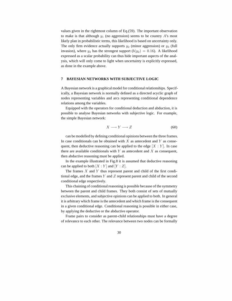
A Bayesian network is a graphical model for conditional relationships. Specif-ically, a Bayesian network is normally defined as a directed acyclic graph ofnodes representing variables and arcs representing conditional dependencerelations among the variables.

Equipped with the operators for conditional deduction and abduction, it ispossible to analyse Bayesian networks with subjective logic. For example,the simple Bayesian network:

X −→ Y −→ Z (60)

can be modelled by defining conditional opinions between thethree frames.In case conditionals can be obtained withX as antecedent andY as conse-quent, then deductive reasoning can be applied to the edge[X : Y ]. In casethere are available conditionals withY as antecedent andX as consequent,then abductive reasoning must be applied.

In the example illustrated in Fig.8 it is assumed that deductive reasoningcan be applied to both[X : Y ] and[Y : Z].

The framesX andY thus represent parent and child of the first condi-tional edge, and the framesY andZ represent parent and child of the secondconditional edge respectively.

This chaining of conditional reasoning is possible becauseof the symmetrybetween the parent and child frames. They both consist of sets of mutuallyexclusive elements, and subjective opinions can be appliedto both. In generalit is arbitrary which frame is the antecedent and which frameis the consequentin a given conditional edge. Conditional reasoning is possible in either case,by applying the deductive or the abductive operator.

Frame pairs to consider as parent-child relationships musthave a degreeof relevance to each other. The relevance between two nodes can be formally

30

FIGURE 8Deductive opinion structure for the Bayesian network of Eq.(60)

expressed as a relevance measure, and is a direct function ofthe condition-als. For probabilistic conditional deduction, the relevance denoted asR(y, x)

between two statesy andx can be defined as:

R(y, x) = |p(y|x) − p(y|x)| . (61)

It can be seen thatR(y, x) ∈ [0, 1], whereR(y, x) = 0 expresses totalirrelevance, andR(y, x) = 1 expresses total relevance betweeny andx.

For conditionals expressed as opinions, the same type of relevance be-tween a given stateyj ∈ Y and a given statexi ∈ X can be defined as:

R(yj , xi) = |E(ωY |xi(yj)) − E(ωY |xj

(yj))| . (62)

The relevance between a child frameY and a given statexi ∈ X of aparent frame can be defined as:

R(Y, xi) = Max[R(yj , xi), j = 1, . . . l] . (63)

31

Finally, the relevance between a child frameY and a parent frameX canbe defined as:

R(Y, X) = Max[R(Y, xi), i = 1, . . . k] . (64)

In our model, the relevance measure of Eq.(64) is the most general.In many situations there can be multiple parents for the samechild, which

requires fusion of the separate child opinions into a singleopinion. The ques-tion then arises which type of fusion is most appropriate. The two most typi-cal situations to consider are the cumulative case and the averaging case.

Cumulative fusion is applicable when independent evidenceis accumu-lated over time such as by continuing observation of outcomes of a process.Averaging fusion is applicable when two sources provide different but inde-pendent opinions so that each opinion is weighed as a function of its certainty.

Both cumulative and averaging situations are encountered in practical sit-uations, and their operators are provided below. The cumulative operator offusing opinions [10] represents a generalisation of the consensus operator[9].

Definition 7 (Cumulative Fusion Operator)Let ωA and ωB be opinions respectively held by agentsA and B over thesame frameX = {xj |j = 1, · · · l}. LetωA⋄B be the opinion such that:

Case I: For uA 6= 0 ∨ uB 6= 0 :

bA⋄B(xj) =bA(xj)u

B+bB(xj)uA

uA+uB−uAuB

uA⋄B = uAuB

uA+uB−uAuB

(65)

Case II: For uA = 0 ∧ uB = 0 :

bA⋄B(xj) = γA bA(xj) + γBbB(xj)

uA⋄B = 0

(66)

where γA = limuA→0uB→0

uB

uA + uBand γB = lim

uA→0uB→0

uA

uA + uB

ThenωA⋄B is called the cumulatively fused bba ofωA andωB, represent-ing the combination of independent opinions ofA andB. By using the symbol‘⊕’ to designate this belief operator, we defineωA⋄B ≡ ωA ⊕ ωB.

The averaging operator for opinions [10] represents a generalisation of theconsensus operator for dependent opinions [13, 16].

32

Theorem 1 (Averaging Fusion Rule)Let ωA and ωB be opinions respectively held by agentsA and B over thesame frameX = {xj | j = 1, · · · , l}. LetωA⋄B be the opinion such that:

Case I: For uA 6= 0 ∨ uB 6= 0 :

bA⋄B(xj) =bA(xj)u

B+bB(xj)uA

uA+uB

uA⋄B = 2uAuB

uA+uB

(67)

Case II: For uA = 0 ∧ uB = 0 :

bA⋄B(xj) = γA bA(xj) + γBbB(xj)

uA⋄B = 0

(68)

where γA = limuA→0uB→0

uB

uA + uBand γB = lim

uA→0uB→0

uA

uA + uB

ThenωA⋄B is called the averaged opinion ofωA andωB, representing thecombination of the dependent opinions ofA andB. By using the symbol ‘⊕’to designate this belief operator, we defineωA⋄B ≡ ωA⊕ωB.

In case of dogmatic opinions, the cumulative and the averaging operatorsare equivalent. This is so because dogmatic opinions must beinterpreted asopinions based on infinite evidence, so that two different opinions necessarilymust be dependent, in which case the averaging operator is applicable.

By fusing child opinions resulting from multiple parents, arbitrarily largeBayesian networks can be constructed. Depending on the situation it must bedecided whether the cumulative or the averaging operator isapplicable. Anexample with three grandparent framesX1, X2, X3, two parent parent framesY1, Y2 and one child frameZ is illustrated in Fig.9 below.

The nodesX1, X2, X3 andY2 represent initial parent frames because theydo not themselves have parents in the model. Opinions about the initial parentnodes represent the input evidence to the model.

When representing Bayesian networks as graphs, the structure of condi-tionals is hidden in the edges, and only the nodes consistingof parent andchildren frames are shown.

When multiple parents can be identified for the same child, there are twoimportant considerations. Firstly, the relative relevance between the child andeach parent, and secondly the relevance or dependence between the parents.

33

FIGURE 9Bayesian network with multiple parent evidence nodes

Strong relevance between child and parents is desirable, and models shouldinclude the strongest child-parent relationships that canbe identified, and forwhich there is evidence directly or potentially available.

Dependence between parents should be avoided as far as possible. A moresubtle and hard to detect dependence can originate from hidden parent nodesoutside the Bayesian network model itself. In this case the parent nodes have ahidden common grand parent node which makes them dependent.Philosoph-ically speaking everything depends on everything in some way, so absoluteindependence is never achievable. There will often be some degree of depen-dence between evidence sources, but which from a practical perspective canbe ignored. When building Bayesian network models it is important to beaware of possible dependencies, and try to select parent evidence nodes thathave the lowest possible degree of dependence.

As an alternative method for managing dependence it could bepossibleto allow different children to share the same parent by fissioning the parentopinion, or alternatively taking dependence into account during the fusionoperation. The latter option can be implemented by applyingthe averagingfusion operator.

It is also possible that evidence opinions provided by experts need to bediscounted due to the analysts doubt in their reliability. This can be done withthe trust transitivity operator¶ of subjective logic.

¶ Also called discounting operator

34

Definition 8 (Trust Transitivity) Let A, B and be two agents whereA’sopinion aboutB’s recommendations is expressed as a binomial opinionωA

B =

{bAB, dA

B, uAB, aA

B}, and letX be a frame whereB’s opinion aboutX is recom-mended toA with the opinionωB

X = {~bBX , uB

X ,~aBX}. LetωA:B

X = {~bA:BX , uA:B

X ,~aA:BX }

be the opinion such that:

bA:BX (xi) = bA

BbBX(xi), for i = 1 . . . k ,

uA:BX = dA

B + uAB + bA

BuBX ,

aA:BX (xi) = aB

X(xi) .

thenωA:BX is calledA’s discounted opinion aboutX . By using the symbol⊗

to denote this operator, trust transitivity can be expressed asωA:BX = ωA

B ⊗

ωBX . 2

The transitivity operator is associative but not commutative. Discountingof opinions through transitivity generally increases the uncertainty mass, andreduces belief masses.

8 DISCUSSION AND CONCLUSION

When faced with complex situations combined with partial ignorance, purehuman cognition and reasoning will often lead to inconsistent and unreliableconclusions. Practical situations where this can happen include medical di-agnostic reasoning, the analysis of financial markets, criminal investigations,and military intelligence analysis, just to name a few examples. In such cases,reasoning based on subjective logic can complement human reasoning to de-rive more consistent and reliable conclusions. The challenge for applyingsubjective logic to the analysis of such situations, is to

• adequately model the situation, and

• determining the evidence needed as input to the model.

The modelling of a given situation includes defining the relevant parent andchild frames, and defining the conditional opinions that relate parent and childframes to each other. Determining the evidence consists of determining theopinions on parent frames from adequate and reliable sources of information.

The results of the analysis are in the form of opinions on child frames ofinterest. These derived opinions can then for example assist a medical practi-tioner to make a more accurate diagnosis, can assist a financial market analystto more realistically predict trends and consequences of actions, can assist

35

police in uncovering crime scenarios, and can assist intelligence analysts inpredicting military scenarios.

Multinomial subjective opinions consist of a Dirichlet bbaand a base ratefunction. We have described methods for conditional deduction and condi-tional abduction with subjective opinions. These methods are based on thegeometric interpretation of opinions as points in pyramidswhere the dimen-sionality of a pyramid is equal to the cardinality of the frame. This interpre-tation provides an intuitive basis for defining conditionalreasoning operatorsfor multinomial opinions. The ability to perform conditional reasoning withmultinomial opinions gives many advantages, such as

• the parent and child frames can be of arbitrary size,

• the reasoning can go in any direction, meaning that for two frameswhere there are conditionally dependent subjective opinions, the choiceof parent and child is arbitrary,

• conditional reasoning can be chained as in Bayesian networks,

• conditional reasoning can be done with arbitrary degrees ofignorancein the opinions,

• the computations are always compatible with classical probabilisticcomputations, and in fact

• the computations are reduced to classical probabilistic computations incase of only using dogmatic opinions.

The cumulative and averaging fusion operators for multinomial opinionsmakes it possible to have multiple parents for each child in Bayesian net-works. In summary, the described methods provide a powerfultool set foranalysing complex situations involving multiple sources of evidence and pos-sibly long chains of reasoning. This allows uncertainty andincomplete knowl-edge to be explicitly expressed in the input opinions, and tobe carried throughthe analysis to the conclusion opinions. In this way the analyst can better ap-preciate the level of uncertainty associated with the derived conclusions.

REFERENCES

[1] F.G. Cozman. (2000). Credal networks.Artif. Intell., 120(2):199–233.

[2] Bruno de Finetti. (1974). The true subjective probability problem. In Carl-Axel Stael vonHolstein, editor,The concept of probability in psychological experiments, pages 15–23,Dordrecht, Holland. D.Reidel Publishing Company.

36

[3] M.R. Diaz. (1981).Topics in the Logic of Relevance. Philosophia Verlag, Munchen.

[4] D. Dubois and H. Prade. (1982). On Several Representations of an Uncertain Bodyof Evidence. In M.M. Gupta and E. Sanchez, editors,Fuzzy Information and DecisionProcesses, pages 167–181. North-Holland.

[5] J.Y. Halpern. (2001). Conditional Plausibility Measures and Bayesian Networks.Journalof Artificial Intelligence Research, 14:359–389.

[6] U. Hoffrage, S. Lindsey, R. Hertwig, and G. Gigerenzer. (December 2000). Communicat-ing statistical information.Science, 290(5500):2261–2262.

[7] A. Jøsang. (December 1997). Artificial reasoning with subjective logic. In AbhayaNayak and Maurice Pagnucco, editors,Proceedings of the 2nd Australian Workshop onCommonsense Reasoning, Perth. Australian Computer Society.

[8] A. Jøsang. (June 2001). A Logic for Uncertain Probabilities. International Journal ofUncertainty, Fuzziness and Knowledge-Based Systems, 9(3):279–311.

[9] A. Jøsang. (October 2002). The Consensus Operator for Combining Beliefs. ArtificialIntelligence Journal, 142(1–2):157–170.

[10] A. Jøsang. (January 2007). Probabilistic Logic Under Uncertainty. InThe Proceedings ofComputing: The Australian Theory Symposium (CATS2007), CRPIT Volume 65, Ballarat,Australia.

[11] A. Jøsang and Z. Elouedi. (November 2007). Interpreting Belief Functions as DirichletDistributions. InThe Proceedings of the 9th European Conference on Symbolic and Quan-titative Approaches to Reasoning with Uncertainty (ECSQARU), Hammamet, Tunisia.

[12] A. Jøsang, R. Hayward, and S. Pope. (January 2006). Trust Network Analysis withSubjective Logic. InProceedings of the29th Australasian Computer Science Conference(ACSC2006), CRPIT Volume 48, Hobart, Australia.

[13] A. Jøsang and S.J. Knapskog. (October 1998). A Metric for Trusted Systems (full paper).In Proceedings of the 21st National Information Systems Security Conference. NSA.

[14] A. Jøsang and D. McAnally. (2004). Multiplication and Comultiplication of Beliefs.International Journal of Approximate Reasoning, 38(1):19–51.

[15] A. Jøsang, S. Pope, and M. Daniel. (2005). Conditional deduction under uncertainty. InProceedings of the 8th European Conference on Symbolic and Quantitative Approaches toReasoning with Uncertainty (ECSQARU 2005).

[16] A. Jøsang, S. Pope, and S. Marsh. (May 2006). Exploring Different Types of TrustPropagation. InProceedings of the 4th International Conference on Trust Management(iTrust), Pisa.

[17] Jonathan Koehler. (1996). The Base Rate Fallacy Reconsidered: Descriptive, Normativeand Methodological Challenges.Behavioral and Brain Sciences, 19.

[18] David Lewis. (1976). Probabilities of Conditionals and Conditional Probabilities.ThePhilosophical Review, 85(3):297–315.

[19] T. Lukasiewicz. (2005). Weak nonmonotonic probabilistic logics. Artif. Intell.,168(1):119–161.

[20] Simon Pope and Audun Jøsang. (2005). Analsysis of Competing Hypotheses using Sub-jective Logic. InProceedings of the 10th International Command and Control Researchand Technology Symposium (ICCRTS). United States Department of Defense Commandand Control Research Program (DoDCCRP).

[21] Frank Ramsey. (1931).The foundations of mathematics, and other logical essays. London,edited by R.B.Braithwaite, Paul, Trench and Trubner. Reprinted 1950, Humanities Press,New York.

37

[22] G. Shafer. (1976).A Mathematical Theory of Evidence. Princeton University Press.

[23] Ph. Smets. (1993). Belief functions: The disjunctive rule of combination and the general-ized Bayesian theorem.International Journal of Approximate Reasoning, 9:1–35.

[24] Ph. Smets. (1998). The transferable belief model for quantified belief representation. InD.M. Gabbay and Ph. Smets, editors,Handbook of Defeasible Reasoning and UncertaintyManagement Systems, Vol.1, pages 267–301. Kluwer, Doordrecht.

[25] Ph. Smets. (2005). Decision Making in the TBM: the Necessity of the Pignistic Transfor-mation. Int. J. Approximate Reasoning, 38:133–147.

[26] Ph. Smets and R. Kennes. (1994). The transferable belief model. Artificial Intelligence,66:191–234.

[27] R. Stalnaker. (1981). Probability and conditionals. In W.L. Harper, R. Stalnaker, andG. Pearce, editors,The University of Western Ontario Series in Philosophy of Science,pages 107–128. D.Riedel Publishing Company, Dordrecht, Holland.

[28] P. Walley. (1991).Statistical Reasoning with Imprecise Probabilities. Chapman and Hall,London.

[29] P. Walley. (1996). Inferences from Multinomial Data: Learning about a Bag of Marbles.Journal of the Royal Statistical Society, 58(1):3–57.

[30] H. Xu and Ph Smets. (1994). Evidential Reasoning with Conditional Belief Functions. InD. Heckermanet al., editors,Proceedings of Uncertainty in Artificial Intelligence (UAI94),pages 598–606. Morgan Kaufmann, San Mateo, California.

[31] H. Xu and Ph Smets. (1996). Reasoning in Evidential Networks with Conditional BeliefFunctions.International Journal of Approximate Reasoning, 14(2–3):155–185.

38