author(s): nobuhiro kiyotaki and john moore …psm509/ulb2012/kiyotakimoorejpe1997.pdf · credit...
TRANSCRIPT

Credit CyclesAuthor(s): Nobuhiro Kiyotaki and John MooreSource: The Journal of Political Economy, Vol. 105, No. 2 (Apr., 1997), pp. 211-248Published by: The University of Chicago PressStable URL: http://www.jstor.org/stable/2138839Accessed: 29/09/2008 11:50
Your use of the JSTOR archive indicates your acceptance of JSTOR's Terms and Conditions of Use, available athttp://www.jstor.org/page/info/about/policies/terms.jsp. JSTOR's Terms and Conditions of Use provides, in part, that unlessyou have obtained prior permission, you may not download an entire issue of a journal or multiple copies of articles, and youmay use content in the JSTOR archive only for your personal, non-commercial use.
Please contact the publisher regarding any further use of this work. Publisher contact information may be obtained athttp://www.jstor.org/action/showPublisher?publisherCode=ucpress.
Each copy of any part of a JSTOR transmission must contain the same copyright notice that appears on the screen or printedpage of such transmission.
JSTOR is a not-for-profit organization founded in 1995 to build trusted digital archives for scholarship. We work with thescholarly community to preserve their work and the materials they rely upon, and to build a common research platform thatpromotes the discovery and use of these resources. For more information about JSTOR, please contact [email protected].
The University of Chicago Press is collaborating with JSTOR to digitize, preserve and extend access to TheJournal of Political Economy.
http://www.jstor.org
Credit Cycles
Nobuhiro Kiyotaki University of Minnesota and Federal Reserve Bank of Minneapolis
John Moore London School of Economics and Heriot-Watt University
We construct a model of a dynamic economy in which lenders can- not force borrowers to repay their debts unless the debts are se- cured. In such an economy, durable assets play a dual role: not only are they factors of production, but they also serve as collateral for loans. The dynamic interaction between credit limits and asset prices turns out to be a powerful transmission mechanism by which the effects of shocks persist, amplify, and spill over to other sectors. We show that small, temporary shocks to technology or income distribution can generate large, persistent fluctuations in output and asset prices.
I. Introduction
This paper is a theoretical study into how credit constraints interact with aggregate economic activity over the business cycle. In particu- lar, for an economy in which credit limits are endogenously deter-
We are indebted to many colleagues and seminar participants. In particular we would like to thank Rao Aiyagari, Fernando Alvarez, John Carlson, Terry Fitzgerald, Mark Gertler, Edward Green, Oliver Hart, Frank Heinemann, Ellen McGrattan, Francois Ortalo-Magn6, Edward Prescott, two referees, and the editor for their thoughtful comments and help. Financial assistance is acknowledged from the U.S. National Science Foundation, the U.K. Economic and Social Research Council, and the Financial Markets Group at the London School of Economics. We are also grate- ful to the Research Department of the Federal Reserve Bank of Minneapolis for its hospitality and support. However, our views are not necessarily those of the bank or the Federal Reserve System.
[Journal of Political Economy, 1997, vol. 105, no. 2] ? 1997 by The University of Chicago. All rights reserved. 0022-3808/97/0502-0003$01.50
211
212 JOURNAL OF POLITICAL ECONOMY
mined, we investigate how relatively small, temporary shocks to tech- nology or income distribution might generate large, persistent fluctuations in output and asset prices. Also we ask whether sector- specific shocks can be contagious, in the sense that their effects spill over to other sectors and get amplified through time.
For this purpose, we construct a model of a dynamic economy in which credit constraints arise naturally because lenders cannot force borrowers to repay their debts unless the debts are secured.' In such an economy, durable assets such as land, buildings, and machinery play a dual role: not only are they factors of production, but they also serve as collateral for loans. Borrowers' credit limits are affected by the prices of the collateralized assets. And at the same time, these prices are affected by the size of the credit limits. The dynamic inter- action between credit limits and asset prices turns out to be a power- ful transmission mechanism by which the effects of shocks persist, amplify, and spread out.
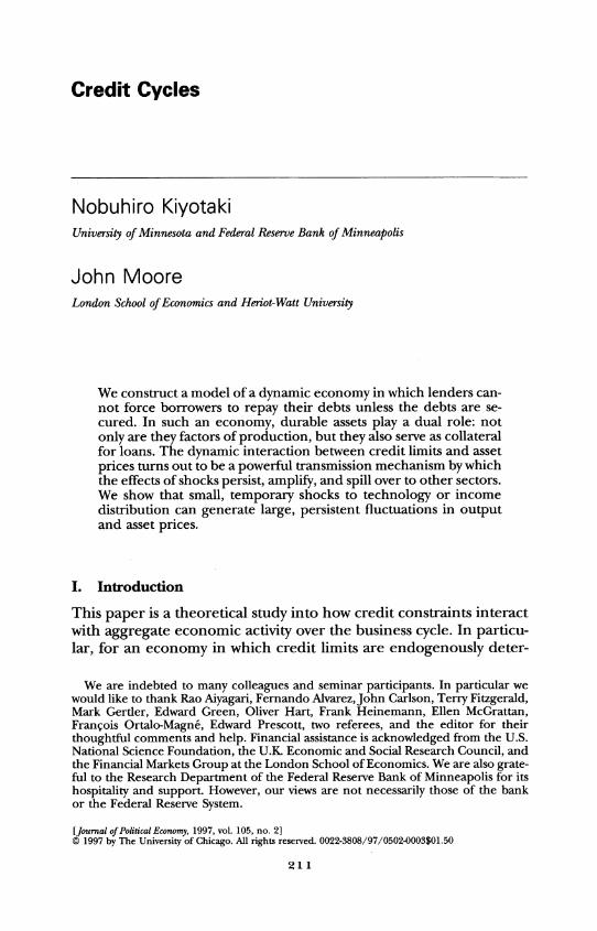
The transmission mechanism works as follows. Consider an econ- omy in which land is used to secure loans as well as to produce out- put, and the total supply of land is fixed. Some firms are credit con- strained, and are highly levered in that they have borrowed heavily against the value of their landholdings, which are their major asset. Other firms are not credit constrained. Suppose that in some period t the firms experience a temporary productivity shock that reduces their net worth. Being unable to borrow more, the credit-con- strained firms are forced to cut back on their investment expendi- ture, including investment in land. This hurts them in the next pe- riod: they earn less revenue, their net worth falls, and, again because of credit constraints, they reduce investment. The knock-on effects continue, with the result that the temporary shock in period t re- duces the constrained firms' demand for land not only in period t but also in periods t + 1, t + 2 .... For the market to clear in each of these periods, the demand for land by the unconstrained firms has to increase, which requires that their opportunity cost, or user cost, of holding land must fall. Given that these firms are uncon- strained, their user cost in each period is simply the difference be- tween that period's land price and the discounted value of the land price in the following period. This anticipated decline in user costs in periods t, t + 1, t + 2, . . . is reflected by a fall in the land price in period t-since price equals the discounted value of future user costs.
The fall in land price in period t has a significant impact on the
'The specific model of debt we use is a simple variant of the model in Hart and Moore (1994).
CREDIT CYCLES 213
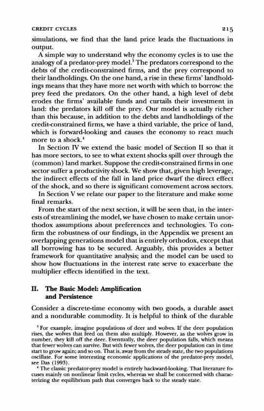
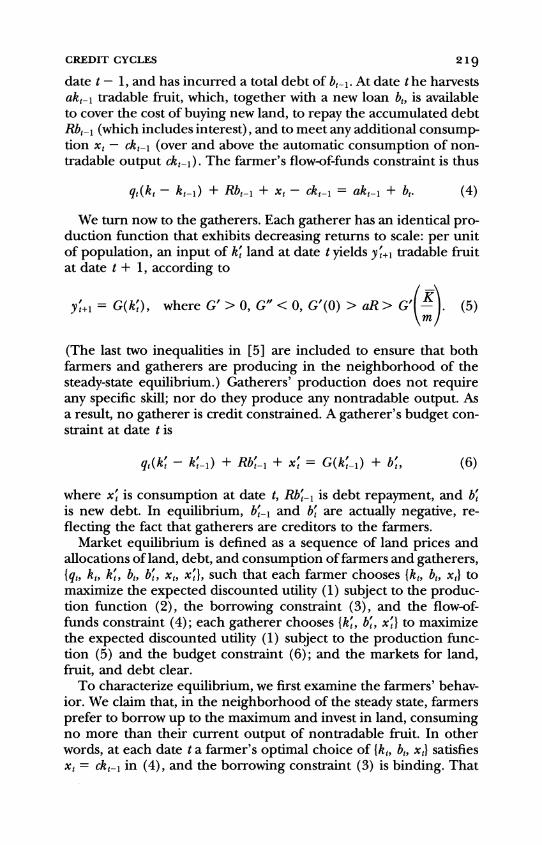
PRESENT FUTURE
date t date t+i date t+2
Negative temporary shock
Net worth of constrained Net worth of constrained Net worth of constrained firms falts finns falls firms falls
Asset demand of constrained Asset demand of constrained Asset demand of constrained firms falls firms falls firms falls
User cost of asset falls User cost of asset falls User cost of asset falls
Asset price falls
FIG. 1
behavior of the constrained firms. They suffer a capital loss on their landholdings, which, because of the high leverage, causes their net worth to drop considerably. As a result, the firms have to make yet deeper cuts in their investment in land. There is an intertemporal multiplier process: the shock to the constrained firms' net worth in period t causes them to cut their demand for land in period t and in subsequent periods; for market equilibrium to be restored, the unconstrained firms' user cost of land is thus anticipated to fall in each of these periods, which leads to a fall in the land price in period t; and this reduces the constrained firms' net worth in period t still further. Persistence and amplification reinforce each other. The process is summarized in figure 1.
In fact, two kinds of multiplier process are exhibited in figure 1, and it is useful to distinguish between them. One is a within-period, or static, multiplier. Consider the left-hand column of figure 1, marked "date t" (ignore any arrows to and from the future). The productivity shock reduces the net worth of the constrained firms, and forces them to cut back their demand for land; the user cost falls to clear the market; and the land price drops by the same amount (keeping the future constant), which lowers the value of the firms' existing landholdings, and reduces their net worth still fur- ther. But this simple intuition misses the much more powerful inter- temporal, or dynamic, multiplier. The future is not constant. As the arrows to the right of the date t column in figure 1 indicate, the overall drop in the land price is the cumulative fall in present and future user costs, stemming from the persistent reductions in the
214 JOURNAL OF POLITICAL ECONOMY
constrained firms' net worth and land demand, which are in turn exacerbated by the fall in land price and net worth in period t.
We find that in our basic model, presented in Section II, the effect of this dynamic multiplier on land price exceeds that of the static multiplier by a factor equal to the inverse of the net real rate of interest. For our basic model, in percentage terms, the change in land price is of the same order of magnitude as the temporary pro- ductivity shock, and the change in land usage exceeds the shock. In the absence of the dynamic multiplier, these changes would be much smaller: the percentage change in price would only be of the order of the shock times the interest rate (i.e., the price would expe- rience only a tiny blip if the length of the period is not long).
A feature of equilibrium is that the marginal productivity of the constrained firms is higher than that of the unconstrained firms- not surprisingly, given that the constrained firms cannot borrow as much as they want. Consequently, any shift in land usage from the constrained to the unconstrained firms leads to a first-order decline in aggregate output. Aggregate productivity, measured by average output per unit of land, also declines, not because there are varia- tions in the underlying technologies (aside from the initial shock), but rather because the change in land use has a compositional ef- fect.2
Our full model is in Section III of the paper. There are two sub- stantive changes to the basic model of Section II. First, we introduce another asset, which, unlike land, depreciates but can be repro- duced. We suppose that the asset has no resale value and so cannot be used to secure loans. This reduces leverage, and hence weakens the contemporaneous effects of a shock. However, there is greater persistence. We also show that if collateralized land is a smaller com- ponent of input, then, in relative terms, land prices respond to a shock more than quantities.
The second change we make to the basic model is that investment is lumpy at the level of the individual firm. Specifically, we suppose that in any period, only a fraction of firms are in a position to invest. This means that only a fraction of the credit-constrained firms cur- rently borrow up to their credit limits; the rest have to await an invest- ment opportunity before reacting to a shock. The economy thus ad- justs more slowly: contemporaneous effects are smaller, but, in contrast to the basic model, the response can build up over time. Moreover, such an economy can exhibit damped oscillations: reces- sions lead to booms, and booms lead to recessions. Investment in the reproducible asset moves with output and land price. And, in
2 This may shed light on why the aggregate Solow residual fluctuates so much over the business cycle.
CREDIT CYCLES 215
simulations, we find that the land price leads the fluctuations in output.
A simple way to understand why the economy cycles is to use the analogy of a predator-prey model.3 The predators correspond to the debts of the credit-constrained firms, and the prey correspond to their landholdings. On the one hand, a rise in these firms' landhold- ings means that they have more net worth with which to borrow: the prey feed the predators. On the other hand, a high level of debt erodes the firms' available funds and curtails their investment in land: the predators kill off the prey. Our model is actually richer than this because, in addition to the debts and landholdings of the credit-constrained firms, we have a third variable, the price of land, which is forward-looking and causes the economy to react much more to a shock.4
In Section IV we extend the basic model of Section II so that it has more sectors, to see to what extent shocks spill over through the (common) land market. Suppose the credit-constrained firms in one sector suffer a productivity shock. We show that, given high leverage, the indirect effects of the fall in land price dwarf the direct effect of the shock, and so there is significant comovement across sectors.
In Section V we relate our paper to the literature and make some final remarks.
From the start of the next section, it will be seen that, in the inter- ests of streamlining the model, we have chosen to make certain unor- thodox assumptions about preferences and technologies. To con- firm the robustness of our findings, in the Appendix we present an overlapping generations model that is entirely orthodox, except that all borrowing has to be secured. Arguably, this provides a better framework for quantitative analysis; and the model can be used to show how fluctuations in the interest rate serve to exacerbate the multiplier effects identified in the text.
II. The Basic Model: Amplification and Persistence
Consider a discrete-time economy with two goods, a durable asset and a nondurable commodity. It is helpful to think of the durable
I For example, imagine populations of deer and wolves. If the deer population rises, the wolves that feed on them also multiply. However, as the wolves grow in number, they kill off the deer. Eventually, the deer population falls, which means that fewer wolves can survive. But with fewer wolves, the deer population can in time start to grow again; and so on. That is, away from the steady state, the two populations oscillate. For some interesting economic applications of the predator-prey model, see Das (1993).
'The classic predator-prey model is entirely backward-looking. That literature fo- cuses mainly on nonlinear limit cycles, whereas we shall be concerned with charac- terizing the equilibrium path that converges back to the steady state.
216 JOURNAL OF POLITICAL ECONOMY
asset as land, which does not depreciate and has a fixed total supply of K. The nondurable commodity may be thought of as fruit, which grows on land but cannot be stored. There is a continuum of infi- nitely lived agents. Some are farmers and some are gatherers, with population sizes one and m, respectively. Both farmers and gatherers produce and eat fruit. They are risk neutral: at date t, the expected utilities of a farmer and a gatherer are
Et( Pxt+s and Et( Xt~s (1)
where x,+s and x'+s are their respective consumptions of fruit at date t + s, and Et denotes expectations formed at date t. The discount factors P and P' both lie strictly between zero and one; and we make the following assumption.
ASSUMPTION 1. P < P'.
We shall see later that assumption 1 ensures that in equilibrium farmers will not want to postpone production, because they are rela- tively impatient.
At each date t there is a competitive spot market in which land is exchanged for fruit at a price of qt. (Throughout, fruit is taken as the numeraire.) The only other market is a one-period credit market in which one unit of fruit at date t is exchanged for a claim to R, units of fruit at date t + 1. We shall see that in equilibrium the farm- ers borrow from the gatherers, and that the rate of interest always equals the gatherers' constant rate of time preference; that is, R, 1 / P= R, say.
Both farmers and gatherers take one period to produce fruit from land, but the farmers differ from the gatherers in their production technologies. We begin with the farmers since they play the central role in the model. Consider any particular farmer. He or she has a constant returns to scale production function:
yt+i = F(kt) (a + c)kt, (2)
where kt is the land used at date t, and yt+i is the output of fruit at date t + 1. Only akt of this output is tradable in the market, however. The rest, ckt, is bruised and cannot be transported, but can be con- sumed by the farmer. We introduce nontradable output in order to avoid the situation in which the farmer continually postpones con- sumption. The ratio a! (a + c) may be thought of as a technological upper bound on his savings rate, which we take to be less than A; that is, we make the following assumption.
CREDIT CYCLES 217
ASSUMPTION 2.
c > (i-1)a.
This inequality is a weak assumption, insofar as 0 is close to one. We shall see later that assumption 2 ensures that in equilibrium the farmer will not want to consume more than the bruised fruit: the overall return from farming, a + c, is high enough that all his trada- ble output is used for investment.5
There are two further critical assumptions we make about farm- ing. First, we assume that each farmer's technology is idiosyncratic in the sense that, once his production has started at date t with land kt, only he has the skill necessary for the land to bear fruit at date t + 1. That is, if the farmer were to withdraw his labor between dates t and t + 1, there would be no fruit output at date t + 1; there would be only the land kt. Second, we assume that a farmer always has the freedom to withdraw his labor; he cannot precommit to work. In the language of Hart and Moore (1994), the farmer's human capital is inalienable.
The upshot of these two assumptions is that if a farmer has a lot of debt, he may find it advantageous to threaten his creditors by withdrawing his labor and repudiating his debt contract. Creditors protect themselves from the threat of repudiation by collateralizing the farmer's land. However, because the land yields no fruit without the farmer's labor, the liquidation value (the outside value) of the land is less than what the land would earn under his control (the inside value). Thus, following a repudiation, it is efficient for the farmer to bribe his creditors into letting him keep the land. In effect, he can renegotiate a smaller loan. The division of surplus in this renegotiation process is moot, but Hart and Moore give an argument to show that the farmer may be able to negotiate the debt down to the liquidation value of the land.6 Creditors know of this possibility
5Notice that we have made two unorthodox modeling choices: we have assumed that agents have linear preferences but different discount factors; and we have in effect assumed that farmers can save only a fraction of their output. Both assump- tions can be dispensed with. In the Appendix we lay out an overlapping generations model in which agents have common concave preferences, and face conventional saving/consumption decisions.
In the text we have taken the shortcut of assuming nonidentical linear preferences and a technologically determined savings rate for the farmers, so that they operate at corner solutions rather than at interior optima. We think that this helps to focus attention on the fact that agents face a sequence of cash flow constraints, which is the crucial difference between our framework and Arrow-Debreu.
6 The case we have in mind is one in which the liquidation (outside) value is greater than the share of the continuation (inside) value that creditors would get if the liquidation option were not available to them-albeit that the liquidation value is less than the total continuation value. In this case, the creditors' "outside option"
218 JOURNAL OF POLITICAL ECONOMY
in advance, and so take care never to allow the size of the debt (gross of interest) to exceed the value of the collateral.7 Specifically, if at date t the farmer has land kt, then he can borrow b, in total, as long as the repayment does not exceed the market value of his land at date t + 1:
Rbt '5 qt+1 ki. (3)
Note that there is no aggregate uncertainty in our model (aside from an initial unanticipated shock), and so, given rational expectations, agents have perfect foresight of future land prices.8
The farmer can expand his scale of production by investing in more land. Consider a farmer who holds kt1 land at the end of
(the option to liquidate) is binding, which pins down the division of surplus in the renegotiation process. For a discussion of the noncooperative foundations of the so-called outside option principle, see Osborne and Rubinstein (1990, sec. 3.12). See the appendix to Hart and Moore (1994) for specific details of the debt renegotia- tion game.
7An alternative, somewhat starker, form of moral hazard would be to assume that the farmers can steal the fruit crop at date t + 1 (see Hart and Moore 1989, 1996). In our basic model, this simple diversion assumption leads to the same borrowing constraint: creditors must never allow a farmer's debt obligations to rise above the value of his land; otherwise he will simply abscond, leaving the land behind but taking all the fruit with him. We have chosen not to tell the story this way because in our full model given in Sec. III there are specific trees growing on the land, which are valuable to the farmer but not to outsiders. Were stealing fruit the only moral hazard problem, the farmer would be able to collateralize his trees as well as his land (since, if he absconded, he would have to leave the trees behind). We are interested in investigating the role of an uncollateralized asset (trees), so we want the farmer to be able to put up only his land as security.
8 Readers may wonder why farmers cannot find some other way to raise capital, e.g., by issuing equity. Unfortunately, given the specific nature of a farmer's technol- ogy, and the fact that he can withdraw his labor, equity holders could not be assured that they would receive a dividend. Debt contracts secured on the farmer's land are the only financial instrument investors can rely on. The same considerations rule out partnerships between farmers, or larger farming cooperatives.
Longer-term debt contracts also offer no additional source of capital, insofar as the farmer can repudiate and renegotiate at any time during the life of a contract. To avoid repudiation and renegotiation, creditors have to ensure that the value of their outstanding loan never exceeds the current liquidation value of the land, i.e., that (3) holds at all times. This means that any credible long-term debt contract can be mimicked by a sequence of short-term debt contracts.
It is worth remarking that if land were rented rather than purchased, this would not change production or allocation along the perfect-foresight equilibrium path of the economy (although the economy would react differently to unanticipated aggregate shocks). We choose to rule out a rental market for land because in our full model in Sec. III farmers plant trees on land, and each farmer's trees are specific to him. If land were rented period by period, then a farmer would be at the mercy of the landlords who own the land on which his specific trees are growing. Given that, along the equilibrium path, the farmer can buy just as much land as he can rent, he is better off purchasing the land outright, so as to avoid being held up by landlords.
CREDIT CYCLES 219
date t - 1, and has incurred a total debt of bt-1. At date t he harvests aknt- tradable fruit, which, together with a new loan bt, is available to cover the cost of buying new land, to repay the accumulated debt Rbt_1 (which includes interest), and to meet any additional consump- tion xt - ckt-1 (over and above the automatic consumption of non- tradable output cktj). The farmer's flow-of-funds constraint is thus
qt(kt-kt-1) + Rbt_1 + xt -ckt- = akt-1 + bt. (4)
We turn now to the gatherers. Each gatherer has an identical pro- duction function that exhibits decreasing returns to scale: per unit of population, an input of k' land at date t yields y'+i tradable fruit at date t + 1, according to
Yt+, = G(k), where G' > 0, G" < 0, G'(O) > aR > G'(J). (5)
(The last two inequalities in [5] are included to ensure that both farmers and gatherers are producing in the neighborhood of the steady-state equilibrium.) Gatherers' production does not require any specific skill; nor do they produce any nontradable output. As a result, no gatherer is credit constrained. A gatherer's budget con- straint at date t is
qt(k -a k1) + Rb`_1
+ x4 = G(k l1) + b, (6)
where x4 is consumption at date t, Rb1_4 is debt repayment, and b' is new debt. In equilibrium, b'_1 and b' are actually negative, re- flecting the fact that gatherers are creditors to the farmers.
Market equilibrium is defined as a sequence of land prices and allocations of land, debt, and consumption of farmers and gatherers, {qt. kt, k, bt, b", xt, x`1, such that each farmer chooses {kt, bt, xJ1 to maximize the expected discounted utility (1) subject to the produc- tion function (2), the borrowing constraint (3), and the flow-of- funds constraint (4); each gatherer chooses {k', b', x41 to maximize the expected discounted utility (1) subject to the production func- tion (5) and the budget constraint (6); and the markets for land, fruit, and debt clear.
To characterize equilibrium, we first examine the farmers' behav- ior. We claim that, in the neighborhood of the steady state, farmers prefer to borrow up to the maximum and invest in land, consuming no more than their current output of nontradable fruit. In other words, at each date t a farmer's optimal choice of {k,, bt, xJI satisfies xt= ckt-1 in (4), and the borrowing constraint (3) is binding. That
220 JOURNAL OF POLITICAL ECONOMY
is, b k = k/R and
t= 1 [(a + qt)kt- lRbt-l]. (7)
qt - - qt~l qRq
The term (a + qt) kt1 - Rb,_1 is the farmer's net worth at the begin- ning of date t; that is, the value of his tradable output and land held from the previous period, net of debt repayment. In effect, (7) says that the farmer uses all his net worth to finance the difference be- tween the price of land, qt, and the amount he can borrow against each unit of land, q,+1/R. This difference, qt - (qt+1/R) = Ut say, can be thought of as the down payment required to purchase a unit of land.
To prove our claim, consider the farmer's marginal unit of trada- ble fruit at date t. He can invest it in l/u, land, which yields c/us nontradable fruit and a/us tradable fruit at date t + 1. The nontrada- ble fruit is consumed; and the tradable fruit is reinvested. This in turn yields (a/lu)(c/lu+?) nontradable fruit and (a/ut)(a/u,+?) tradable fruit at date t + 2; and so on. Now we appeal to the principle of unimprovability, which says that we need consider only single devi- ations at date t to show that this investment strategy is optimal.9 There are two alternatives open to the farmer at date t. Either he can save the marginal unit-equivalently, reduce his current bor- rowing by one-and use the return R to commence a strategy of maximum levered investment from date t + 1 onward. Or he can simply consume the marginal unit. His choice boils down to choos- ing one of the following consumption paths:
c a c a a c invest: 0, c, , , a (8a)
Ut Ut Ut+1 Ut Ut+1 Ut+2
C a c save: 0, 0, R , R ... (8b)
Ut+1 Ut+1 Ut+2
consume: 1, 0, 0, 0, ... (8c)
at dates t, t + 1, t + 2, t + 3, . .. , respectively. To complete the proof, we need to confirm that, given the farmer's discount factor P, consumption path (8a) offers a strictly higher utility than (8b) or (8c), in the neighborhood of the steady state. We shall be in a posi- tion to show this once we have found the steady-state value of ut in (13a) below.
9On the principle of unimprovability, see, e.g., proposition 4 in app. 2 of Kreps (1990).
CREDIT CYCLES 221
Since the optimal k, and b, are linear in k,_1 and b,-l, we can aggre- gate across farmers to find the equations of motion of the aggregate landholding and borrowing, K, and B, say, of the farming sector:
Kt =-[(a + qt)KtI- RB,1], (9) Ut
Bt = R qt+l Kt. ((10) R
Notice from (9) that if, for example, present and future land prices, qt and qt+i, were to rise by 1 percent (so that ut also rises by 1 percent), then the farmers' demand for land at date t would also rise-provided that leverage is sufficient that debt repayments RB,-l exceed current output aK,-1, which will be true in equilibrium. The usual notion that a higher land price qt reduces the farmers' demand is more than offset by the facts that (i) they can borrow more when qt+i is higher, and (ii) their net worth increases as qt rises. Even though the required down payment, ut, per unit of land rises propor- tionately with qt and qt+i, the farmers' net worth is increasing more than proportionately with qt because of the leverage effect of the outstanding debt.
Next we examine the gatherers' behavior. A gatherer is not credit constrained, and so his or her demand for land is determined at the point at which the present value of the marginal product of land is equal to the opportunity cost, or user cost, of holding land, qt - (qt+?/R) = ut:
- G'(k') = ut. (11) R
Notice the dual role played by ut in the model: not only is it the gatherers' opportunity cost of holding a unit of land, but it also hap- pens to be the required down payment per unit of land held by the farmers."1
Finally, we consider market clearing. Since all the gatherers have identical production functions, their aggregate demand for land
'"We say "happens to be" because a borrowing constraint different from (3) would yield different expressions for k, and K, in (7) and (9). For example, we might suppose that, out of equilibrium, if a farmer were to repudiate his debt contract and the renegotiation of a new contract with his creditors were to break down, then there would be a (proportional) transactions cost r associated with disposing of his land. That is, the liquidation value would be multiplied by 1 - t. The borrowing constraint (3) would become Rb, ' (1 - r) qt+I kt, and the denominator on the right- hand sides of (7) and (9) would read qt - [(1 - r) qt+l /R]. Although the analysis of the model would then be slightly different, its behavior would be similar.
222 JOURNAL OF POLITICAL ECONOMY
equals kt times their population m. The sum of the aggregate de- mands for land by the farmers and gatherers is equal to the total supply; that is, Kt + mkt = K. Thus, from (11), we obtain the land market equilibrium condition
ut = qt-- qt+l = u(Kt), where u(K) GI K)] (12)
The function u(.) is increasing: if the farmers' demand for land, Kt, goes up, then in order for the land market to clear, the gatherers' demand has to be choked off by a rise in the user cost, ut. Given that the gatherers have linear preferences and are not credit con- strained, in equilibrium they must be indifferent about any path of consumption and debt (or credit); and so the interest rate equals their rate of time preference (R = 1/,'). Moreover, given (12), the markets for fruit and credit are in equilibrium by Walras' law.
We restrict attention to perfect-foresight equilibria in which, with- out unanticipated shocks, the expectations of future variables realize themselves. For a given level of farmers' landholding and debt at the previous date, Kt-1 and Bt-1, an equilibrium from date t onward is characterized by the path of land price, farmers' landholding, and debt, {(qt+s, Kt+5, Bt+,) Is - 01, satisfying equations (9), (10), and (12) at dates t, t + 1, t + 2, .... We also rule out exploding bubbles in the land price by making the following assumption.
ASSUMPTION 3. lim5s- Et(Rsqt+s) = 0. Given assumption 3, it turns out that there is a locally unique per-
fect-foresight equilibrium path starting from initial values Kt-1 and Bt-1 in the neighborhood of the steady state.
Before we turn to dynamics, it is useful to look at the steady-state equilibrium. From equations (9), (10), and (12), it is easily shown that there is a unique steady state, (q*, K*, B*), with associated steady-state user cost u*, where
Rq =u = a, (13a) R
q
-G";-(K- K*)] = u*, (13b)
B*= a K*. (13c) R- 1
In the steady state, the farmers' tradable output, aK*, is just enough to cover the interest on their debt, (R - 1)B*. Equivalently, the re- quired down payment per unit of land, u*, equals the farmers' pro-
CREDIT CYCLES 223
D
G'(K'/m)
a+c A t
Ra............ .........................
," .~~~~~~"
K* Kt K0 K
Farmers Gatherers
K K'
FIG. 2
ductivity of tradable output, a. As a result, farms neither expand nor shrink."
We are now in a position to compare consumption paths (8a), (8b), and (8c). In the steady state, the user cost equals a; and so, given the farmer's discount factor P, investment gives him dis- counted utility Pc/ (1 - ) a, saving gives RP2 c/ (1 - ) a, and con- sumption gives one. By assumption 1, investment strictly dominates saving; and by assumption 2, investment strictly dominates consump- tion. This completes the proof of our earlier claim about farmers' optimal behavior in the neighborhood of the steady state.
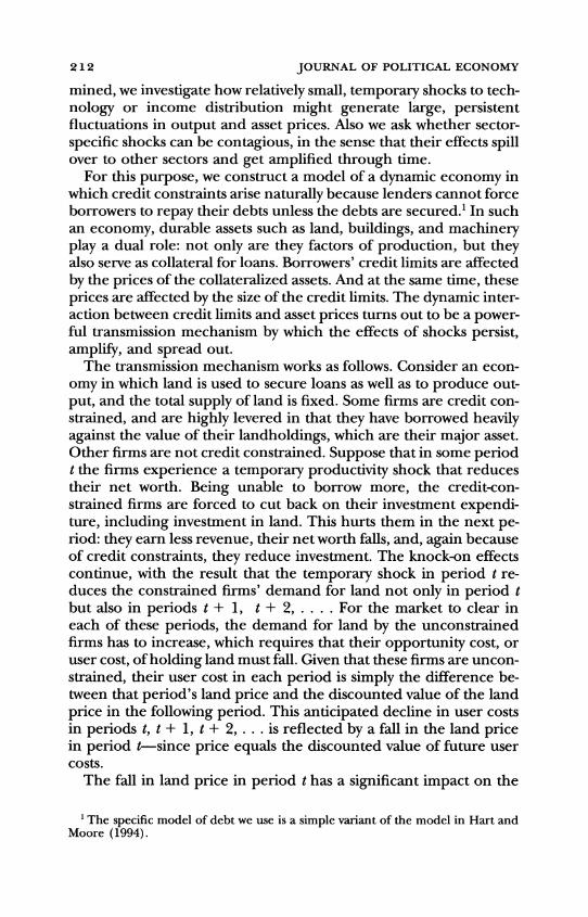
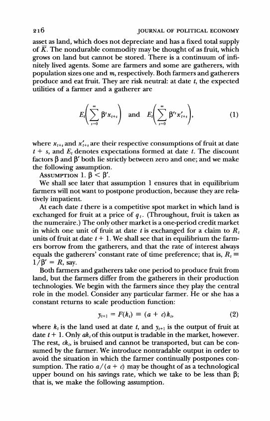
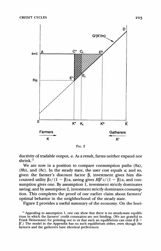
Figure 2 provides a useful summary of the economy. On the hori-
" Appealing to assumption 1, one can show that there is no steady-state equilib- rium in which the farmers' credit constraints are not binding. (We are grateful to Frank Heinemann for pointing out to us that such an equilibrium can exist if P = IV.) The model in the Appendix has no such equilibrium either, even though the farmers and the gatherers have identical preferences.
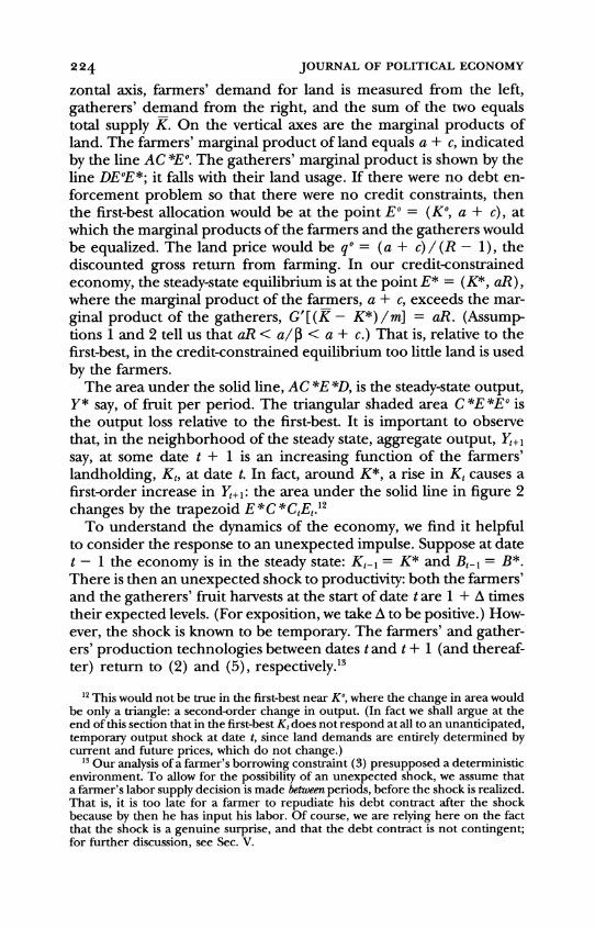
224 JOURNAL OF POLITICAL ECONOMY
zontal axis, farmers' demand for land is measured from the left, gatherers' demand from the right, and the sum of the two equals total supply K. On the vertical axes are the marginal products of land. The farmers' marginal product of land equals a + c, indicated by the line AC *Eo. The gatherers' marginal product is shown by the line DE?E*; it falls with their land usage. If there were no debt en- forcement problem so that there were no credit constraints, then the first-best allocation would be at the point E = (K", a + c), at which the marginal products of the farmers and the gatherers would be equalized. The land price would be q" = (a + c)/(R - 1), the discounted gross return from farming. In our credit-constrained economy, the steady-state equilibrium is at the point E* = (K*, aR), where the marginal product of the farmers, a + c, exceeds the mar- ginal product of the gatherers, G'[I(K - K*) /m] = aR. (Assump- tions 1 and 2 tell us that aR < a/,8 < a + c.) That is, relative to the first-best, in the credit-constrained equilibrium too little land is used by the farmers.
The area under the solid line, AC *E *D, is the steady-state output, Y* say, of fruit per period. The triangular shaded area C *E *Eo is the output loss relative to the first-best. It is important to observe that, in the neighborhood of the steady state, aggregate output, Y,+, say, at some date t + 1 is an increasing function of the farmers' landholding, K&, at date t. In fact, around K*, a rise in K, causes a first-order increase in Y,+,: the area under the solid line in figure 2 changes by the trapezoid E *C *CtEt.l2
To understand the dynamics of the economy, we find it helpful to consider the response to an unexpected impulse. Suppose at date t - 1 the economy is in the steady state: K,-, = K* and B,_l = B*. There is then an unexpected shock to productivity: both the farmers' and the gatherers' fruit harvests at the start of date t are 1 + A times their expected levels. (For exposition, we take A to be positive.) How- ever, the shock is known to be temporary. The farmers' and gather- ers' production technologies between dates t and t + 1 (and thereaf- ter) return to (2) and (5), respectively.'3
12 This would not be true in the first-best near K0, where the change in area would be only a triangle: a second-order change in output. (In fact we shall argue at the end of this section that in the first-best K, does not respond at all to an unanticipated, temporary output shock at date t, since land demands are entirely determined by current and future prices, which do not change.)
13 Our analysis of a farmer's borrowing constraint (3) presupposed a deterministic environment. To allow for the possibility of an unexpected shock, we assume that a farmer's labor supply decision is made between periods, before the shock is realized. That is, it is too late for a farmer to repudiate his debt contract after the shock because by then he has input his labor. Of course, we are relying here on the fact that the shock is a genuine surprise, and that the debt contract is not contingent; for further discussion, see Sec. V.
CREDIT CYCLES 225
Combining the market-clearing condition (12) with the farmers' demand for land (9) and their borrowing constraint (10) at dates t9 t+ 1, t+ 2, .. , we obtain
u (K,)K = (a + Aa + qt - q*)K* (date t) (14a)
and
u(Kt+s)Kt+s = aKt+s-l for s 2 1 (dates t + 1, t + 2, . . .). (14b)
Equations (14) say that at each date the farmers can hold land up to the point Kat which the required down payment, u(K) K, is cov- ered by their net worth. Notice that in (14b), at each date t + s (s ' 1), the farmers' net worth isjust their current output of tradable fruit, aKt+s-1: from the borrowing constraint at date t + s - 1, the value of the farmers' land at date t + s is exactly offset by the amount of debt outstanding. In (14a), however, we see that the farmers' net worth at date t-just after the shock hits-is more than simply their current output, (1 + A) aK*, because qt jumps in response to the shock and they enjoy unexpected capital gains, (qt - q*) K*, on their landholdings (the value of land held from date t - 1 is now qtK*, while the debt repayment is RB* = q* K*).
To find closed-form expressions for the new equilibrium path, we take A to be small and linearize around the steady state. Let Xt de- note the proportional change, (X, - X*) /X*, in a variable Xt rel- ative to its steady-state value X*. Then, using the fact that (R - 1)q*/R = = a, we obtain from equations (14)
1 + K, = A +____ (date t) (15a)
and
(1 + Kt+S= Kt+s-l for s 2 1 (dates t + 1, t ... .), (15b)
where ri > 0 denotes the elasticity of the residual supply of land to the farmers with respect to the user cost at the steady state.14
The right-hand side of (15a) divides the change in the farmers'
14 That is,
1 dlog u(K) dlog G'(k') K*
11 d log K K=K* d log k' k'=(1/m)(K-K*) K- K*
which is the elasticity of the gatherers' marginal product of land times the ratio of the farmers' to the gatherers' landholdings in the steady state. Given our assumption that G" < 0, Tj is positive.
226 JOURNAL OF POLITICAL ECONOMY
net worth at date t into two components: the direct effect of the productivity shock, A; and the indirect effect of the capital gain aris- ing from the unexpected rise in price, qt. Crucially, the impact of qt is scaled up by the factor R/ (R - 1) because of leverage: the farmers' steady-state net worth equals aK*; and so, ceteris paribus, a 1 percent rise in qt increases their net worth by q*K*/aK* = R/ (R - 1) per- cent.
The factor 1 + (1/i) on the left-hand sides of (15) reflects the fact that as the farmers' land demand rises, the user cost must rise for the market to clear; and this in turn partially chokes off the in- crease in the farmers' demand. The key point to note from (15b) is that, except for the limit case of a perfectly inelastic supply (TI = 0), the effect of a shock persists into the future. The reason is that the farmers' ability to invest at each date t + s is determined by how much down payment they can afford from their net worth at that date, which in turn is historically determined by their level of pro- duction at the previous date t + s - 1.
It remains to find out the size of the initial change in the farmers' landholdings, K&, which, from (15a), is jointly determined with the change in land price, qt. Now assumption 3 together with (12) tells us that the land price qt is the discounted sum of future user costs, ut+S = u(Kt+s), s 0 O. Linearizing around the steady state and then substituting from (15b), we obtain
qt R s Kt+s = R 1 TI Kt. (16)
R1 + Tl
The multiplier {1 - [E1/R(1 + Il)]}- in (16) captures the effects of persistence in the farmers' landholdings, and has a dramatic effect on the sizes of qt and Kt. Solve (15a) and (16) to find q, and Kt in terms of the size of the shock A:
, 1 qt = - A, (17)
Kt= (1 i ( R 1_)A. (18)
Equation (17) tells us that, in percentage terms, the effect on the land price at date t is of the same order of magnitude as the temporary productivity shock! As a result, the effect of the shock on the farmers' landholdings at date t is large: the multiplier in (18) exceeds unity, and can do so by a sizable margin, thanks to the factor R/ (R - 1).
CREDIT CYCLES 227
In terms of (15a), the indirect effect of qt, scaled up by the leverage factor R/ (R - 1), is easily enough to ensure that the overall effect on K, is more than one-for-one.'5"6
Recall the distinction we drew in the Introduction between the static and dynamic multipliers. Imagine, hypothetically, that there were no dynamic multiplier. That is, suppose qt+i were artificially pegged at the steady-state level q*. Equation (15a) would remain unchanged. However, the right-hand side of (16) would contain only the first term of the summation-the term relating to the change in user cost at date t-so that the multiplier {1 - [iI/R(I + Ti) ] 1- would disappear. Combining the modified equation, qt = I(R -
1) /iR] Kt, with (15a), we solve for q, and Kt:
qtlqt+l=q* = R1 -A, (17')
Ktlqt+,=q* = A. (18')
These are the changes in the land price and the farmers' landhold- ings that can be traced to the static multiplier alone. Subtracting (17') from (17), we find that the additional movement in land price attributable to the dynamic multiplier is 1 / (R - 1) times the move-
15 The direct effect of the productivity shock A is less than one-for-one because a rise in user cost u, chokes it off. Notice that for inelastic supply (11 < 1), the indirect effect is particularly marked. We know from (17) that a 1 percent productivity shock leads to a more than 1 percent increase in land price. However, the effects are shorter-lived: from (15b) we see that the decay factor is 1 / (1 + 11) < 1/2. Conversely, for elastic supply the indirect effect is less marked, and the impact on land price is less than proportional; however, there is more persistence. In the limit, as 11 -* -, there is no indirect effect: a 1 percent productivity shock leads to a 1 percent change in the farmers' landholdings, and there is no change in land price; but there is complete persistence.
16 Because of the large multiplier effects, the nonlinear equilibrium system com- prising (14) and the land price equation
qt= R-5u(K,+,) s=O
can have multiple dynamic equilibria, even though the linearized system (15), (16) has a unique equilibrium. Solving (14b) as K,+s = t (K,+s-1) or Kt+s = Os(Kt), we can combine (14a) and the equation above to obtain
u(K,)K, - (a + A a)K* - R-s[u(Os(Kt)) - a]K* = 0. s=O
This can have a solution K, outside a neighborhood of K*. (This can be true even when there is no shock [A = 0].) In particular, if Ru(O) < a, then there is another solution K, that is considerably less than K*. Intuitively, if the farmers' future land- holdings are expected to be small, then currently the land price will be low, the farmers will have little net worth, and they will be unable to borrow much to buy land-which in turn justifies the expectation that their future landholdings will be small. Eventually, the economy returns to the unique steady state.
228 JOURNAL OF POLITICAL ECONOMY
ment due to the static multiplier. And a comparison of (18) with (18') shows that the dynamic multiplier has a similarly large propor- tional effect on the farmers' landholdings.'7
As we saw in figure 2, aggregate fruit output-the combined har- vest of the farmers and gatherers-moves together with the farmers' landholdings, since the farmers' marginal product is higher than the gatherers'. It is straightforward to show that at each date t + s the proportional change in aggregate output, Yt+s, is given by
_ a+c-Ra(a+ c)KKt+sl for*s-. (19)
The term (a + c - Ra) / (a + c) reflects the difference between the farmers' productivity (equal to a + c) and the gatherers' productivity (equal to Ra in the steady state). The ratio (a + c) K*/ Y* is the share of the farmers' output. If aggregate productivity were measured by Yt+s/ K, it would be persistently above its steady-state level, even though there are no positive productivity shocks after date t. The explanation lies in a composition effect: there is a persistent change in land usage between farmers and gatherers, which is reflected in increased aggregate output.
One interesting issue is how the economy would respond to other kinds of shock. In particular, suppose that instead of a temporary productivity shock at date t, the economy experiences an unantici- pated, one-time reduction in the value of debt obligations. This debt reduction has the same qualitative effect as the temporary productiv- ity increase (except that there is no increase in output at the ini- tial date). Quantitatively, however, since the outstanding debt of the farmers is R/ (R - 1) times their output of tradable fruit (in the steady state, RB*/aK* = R/I[R - 1]), a reduction of only (R - 1) /R percent in the value of their debt obligations is enough to generate the same effects as a 1 percent temporary productivity shock.'8
To close this section, let us ask what would happen in the first- best economy, where there are no credit constraints. Consider the effect of the same unanticipated, temporary productivity shock A at
7 A less artificial way to get qt+I = q* would be to have a second, negative, productiv- ity shock, -A, at date t + 1 (anticipated at date t). That is to say, the static multiplier has the same effect as two equal but opposite shocks hitting the economy in succes- sion.
8 Although our model does not have money, so we cannot analyze monetary pol- icy per se, one possible monetary transmission mechanism would be through the redistribution of wealth between debtors and creditors, as emphasized by Fisher (1933) and Tobin (1980). If debt contracts were uncontingent and nominal, and if an unexpected increase in the money supply increased the nominal price level, then it would reduce the real burden of outstanding debt.
CREDIT CYCLES 229
date t. Aggregate output Yt would rise by the factor A. But there would be no effect on the land price qt or the land usage Kt; they would stay at qO and K". Nor would there be any change to future prices and production. The point is that in the first-best economy, all agents are unconstrained in the credit market, and prices and production are unaffected by changes to net worth. This is in marked contrast to what we have seen happens in the credit-con- strained economy, where qt and Kt (and hence Yt+1) increase signifi- candy, and these increases persist into the future.
III. The Full Model: Investment and Cycles
The basic model of Section II has a number of limitations. The only "investment" occurs in land itself; and although land changes hands between farmers and gatherers, aggregate investment is automati- cally zero because the total land supply is fixed. Also, the impulse response of the economy to a shock is arguably too dramatic and short-lived (especially when the residual supply of land to the farm- ers is inelastic). The reason is that the leverage effect is so strong: in the steady state the farmers' debt/asset ratio is 1 /R, which is un- reasonably high if the length of the period is not long. Finally, the simplicity of the model hides certain important dynamics.
In this section we extend the basic model to overcome these limi- tations. There are two substantive changes. First, we introduce repro- ducible capital, trees, into the farmers' production function. A farmer plants fruit in his land to grow trees, which later yield fruit. Land does not depreciate, but trees do. As the farmer must replenish his stock of trees by planting more fruit, the planted fruit can be thought of as investment. We shall see that aggregate investment is always positive, and fluctuates together with aggregate output and land price. Trees are assumed to be specific to the farmer who planted them, and so, we shall argue, cannot be used as collateral- unlike the land on which they are grown. Farmers' debt/asset ratios are thus reduced, which weakens the leverage effect. The contempo- raneous response of the economy to a shock is less dramatic, but there is more persistence. We further show that thi presence of the uncollateralized trees causes there to be greater movement in land price, relative to quantities.
The second substantive change we make to the model of Section II is that in each period only a fraction of the farmers have an invest- ment opportunity. The other farmers are unable to invest, and in- stead use their revenues partially to pay off their debts. Ex post, then, farmers are heterogeneous. The probabilistic investment assump- tion simply captures the idea that, at the level of the individual enter-
230 JOURNAL OF POLITICAL ECONOMY
prise, investment in fixed assets is typically occasional and lumpy."9 Since it is no longer the case that all farmers are borrowing up to their credit limits, in aggregate the value of the farmers' debt repay- ments is strictly smaller than the value of their collateralized asset, land. We shall see that this uncoupling of the farmers' aggregate borrowing from their aggregate landholdings allows for rich dy- namic interactions among qt, K:, and B1, and can lead to cycles.
To understand the specifics of the model, consider a particular farmer. We say that his land is cultivated if he has trees growing on it. If he works on k,-l units of cultivated land at date t - 1, he will produce akt1 tradable fruit and ckt1 nontradable fruit at date t- just as in Section II. A fraction 1 - X of the trees are assumed to die by date t, and so this part of the land is no longer cultivated. This does not mean that the land cannot be used; it may be used by gatherers, or it may be cultivated again, possibly by another farmer.
In order to increase his holding of cultivated land at date t from Xk,-l to k1, the farmer must plant 0 (k, - X kl) fruit, as well as acquire k,- kl more land.20 However, we assume that a new investment opportunity to plant fruit arises only with probability R. With proba- bility 1 - x, the farmer is unable to invest, so the scale of his op- erations is limited to Xk,-l and (in equilibrium) he sells off the (1 - A)kl uncultivated land. We assume that the arrival of invest- ment opportunities is independent both across farmers and through time (hence, because there is a continuum of farmers, there is no aggregate uncertainty)).21
We make three assumptions about the parameters. In assumption 4, the tradable output is at least enough to replant the depreciated trees.
ASSUMPTION 4. a > (1 - X)0. In assumption 5, the arrival rate of an investment opportunity is
not too small.
9 For empirical evidence on this, see, e.g., Doms and Dunn (1994). Investment by individual firms may be lumpy because of fixed costs-an idea that clearly war- rants a full analysis. However, in the interests of keeping our aggregate model simple, we rely on the assumption of a probabilistic investment opportunity.
20 Formally, the farmers have a one-period Leontief production function. There are two inputs, land and trees, in 1:1 fixed proportion. There are four outputs: land, trees, tradable fruit, and nontradable fruit, in fixed proportions 1 :X: a: c. In addition, the farmers have an instantaneous technology for growing trees: 4 fruit make one tree.
21 An alternative, possibly more natural, specification of the depreciation process is that the entire stock of trees of an individual farmer dies with probability 1 -X, and survives with probability X. (For example, there may be a storm or a disease.) These shocks are independent across farmers and through time, and are also inde- pendent of the arrival of investment opportunities. In aggregate, this alternative specification leads to the same equilibrium paths as the model in the text.
CREDIT CYCLES 231
ASSUMPTION 5. n > 1 - (1/R). Finally, assumption 2' strengthens assumption 2. ASSUMPTION 2'.
c 1 1- RX(1-r {1l(a + X?).
PR[Xr + (1-)(1-R + rR)] (P 1
Notice that assumptions 5 and 2' are both weak assumptions, given that P and R are typically close to one.
We suppose that each farmer grows his own specific trees, and only he has the skill necessary for them to bear fruit (the other farm- ers do not know how to prune them). This means that, a farmer having sunk the cost (in terms of fruit) of growing trees, there is a wedge between the inside value to him of his cultivated land and the outside value of the land to everyone else. Also, we continue to assume that a farmer's specific human capital is inalienable: he can- not precommit to tending his trees. And so, from the argument given earlier, we deduce that creditors will be unwilling to lend be- yond the limit in (3). That is, only land can serve as collateral.
The rest of the model is exactly the same as in Section II. To sum up, we have made two changes to the basic model. First, the farmer's flow-of-funds constraint (4) now includes the investment in trees,
(kt -Xkt-1):
qt(kt-kt-1) + 0(kt - Xkt1) + Rbt-1 + xt -ckt- = akt-1 + bt. (20)
Second, at each date t, with probability 1 - x, a farmer may now face the additional technological constraint kt ' Xkt-l.
It is worth observing that, at the risk of laboring the exposition, we could have made these changes one at a time. We could have introduced trees into the model without introducing heterogeneity (O > 0, n = 1). Equally, we could have introduced heterogeneity into the model without introducing trees (n < 1, 0 = 0). Later we shall isolate the particular contributions that i and 0 make to the dynamics of the model.
To characterize equilibrium, we need to examine the farmers' be- havior. Start with a farmer who can invest at date t. We claim that he will choose to borrow up to the maximum and invest in land, consuming no more than his current output of nontradable fruit. Specifically, we claim that, in the neighborhood of the steady-state equilibrium, by assumption 1 it is strictly better for the farmer to invest than to save, and by assumption 2' it is strictly better for him to invest than to consume. (For a proof of these claims, see n. 22 below.) That is, the credit constraint (3) is binding, and xt = ckt-l; so it follows from (20) that
232 JOURNAL OF POLITICAL ECONOMY
t= [(a + qt + Xo)kt- - Rbt-1]. (21)
+ qt- qt+l
The term in brackets is the farmer's net worth, which, as we define it, includes the replacement cost of the Xkt-1 trees inherited from date t - 1. (The liquidation value of his assets would exclude the Xokt-l term since the trees have no public value.) The investing farmer uses his net worth to finance the difference between the unit cost of investment, 0 + qt, and the amount he can borrow against a unit of land, qt+1/R.
Next consider a farmer who cannot invest at date t. We claim that he will choose not to divest, that is, he will set
kt= Xkt-1; (22)
and, by assumption 2', he will use his tradable output, akt-1, together with his receipts from land sales, qt( 1 - X)kt1, to pay off his debt rather than consume more than the bruised fruit ckt .22,23
22 To prove these claims, we again appeal to the principle of unimprovability and consider only single deviations at date t. At the start of any subsequent date-after harvest, but before we know whether there is an investment opportunity at that date-let V(L, T) denote a farmer's steady-state expected discounted utility, where L denotes the liquidation (i.e., public) value of his assets, and T denotes his tree holding. Since trees die at the rate 1 - X, we deduce that he must have cultivated Tb. land at the previous date, and will thus have a harvest of aT/X tradable fruit and cT/X nontradable fruit. The liquidation value L comprises the tradable fruit harvest, together with the value of the land (without trees), net of debt repayments. Assuming that from date t + 1 onward the farmer uses the strategy given in the text, we can solve for V(L, T) from the Bellman equation
V(L, T) = T+ on a.+ o* 7w X + 0(I-+(1-7)V(RL + aT-Ru*T, 7T),
where u* is the steady-state user cost of land (see [25a] below). The value function V(L, T) takes the linear form LcLL + TaT, where the constants cLL and aT are found by the method of undetermined coefficients. Now consider the farmer's choices at date t. On the one hand, suppose that he has an investment opportunity. If he uses his marginal unit of tradable fruit as a down payment for investment, then he gains an expected discounted utility [8a/l ( + U*) ] aL + [Pk/ (O + U*) ] aT. If he saves, he gains PRaL. If he consumes, he gains one. It can be shown that, by assumption 1, investment strictly dominates saving; and, by assumption 2', investment strictly dominates consumption. On the other hand, suppose that the farmer cannot invest at date t. Then he will strictly prefer to save rather than to consume his marginal unit of tradable fruit if PRaL > 1. It can be shown that this also is implied by assump- tion 2'. Divestment is not optimal, since, inter alia, the farmer would waste his trees.
23 Note that a noninvesting farmer's new level of indebtedness is given by Rb_1 - ak_1 - qt(l - X)k,-. We need to show that the farmer can borrow this much. With assumption 5, it is straightforward to confirm that, in the neighborhood of the steady-state equilibrium, the borrowing constraint (3) is always strictly satisfied. This is equivalent to saying that the farmer's landholding after he has been forced to shrink it back (the right-hand side of [22] ) is strictly less than what it would have been had he been able to invest (the right-hand side of [21]). In fact, if by chance an individual farmer has a long history of no opportunity to invest, he may eventually
CREDIT CYCLES 233
Expressions (21) and (22) have the great virtue that they are lin- ear in kt1 and b,-l. Hence we can aggregate across farmers and ap- peal to the law of large numbers to derive the equations of motion for the farmers' aggregate landholding and borrowing, K, and Bt, without having to keep track of the distribution of the individual farmers' k,'s and b,'s. Since the population of farmers is unity, with a fraction X investing and a fraction 1 - X not investing, we have
Kt= (1 -)1Kt_) (23)
+ X [(a + qt + XO)Kt- - RB,-l].
+ qt - qt+l
And since no farmer consumes more than his nontradable output, we deduce from the flow-of-funds constraint (20) that
Bt = RBt-l + qt(Kt - Kt1) + O(Kt - XKI) - aK,-1. (24)
Notice that (23) and (24) generalize (9) and (10) to the case in which p > 0 and X < 1.
The land market-clearing condition for the user cost ut = qt -
(qt+I/R), equation (12), is unchanged. Thus, for predetermined lev- els of the farmers' landholding and debt at the previous date, Kt-I and B,-1, an equilibrium from date t onward is characterized by the path of land price, farmers' landholding, and debt, { (qt+s, Kt+s Bt+s) is ? 0), satisfying (12), (23), and (24) at dates t, t + 1, t + 2, .... These equations constitute a first-order nonlinear system. There is a unique steady state, (q*, K*, B*), with associated steady-state user cost u*,, where
R-1 q* = -a = a- (1- ) (1 -R + 7tR) (25a) R Ad1 + (1 (1-R + 7cR)
RG'I-(K- K*)I *, (25b)
B= (a- + Xo)K*. (25c) R-1
Assumptions 4 and 5 ensure that these steady-state values are posi- tive.
To examine the dynamics, we linearize around the steady state.24
become a net creditor (i.e., his b, may become negative) -whereas his landholding is always positive and is declining geometrically at the rate X.
24 For details of what follows, see the appendix of Kiyotaki and Moore (1995).
234 JOURNAL OF POLITICAL ECONOMY
We continue to assume assumption 3, to rule out exploding bubbles in the land price. It can be shown that one eigenvalue equals R > 1, which corresponds to an explosive path; and that the other two eigenvalues will be stable and complex if
where
a+, R(l -7) 0
X XX2X + (1 - X)(1 -R + iR) + IX2C- (1- X)212 L1- XR(1-I) J
and 0 u*/ (? + u*), the steady-state ratio of the user cost of land to the farmers' required down payment per unit of investment. (Note that 0 < 0 < 1. In Sec. II, 0 was unity.) From now on, we assume that the condition above holds. The argument of the first square root is positive by assumption 5; and the argument of the second square root will be positive insofar as X is close to one. If X is not too close to zero or one, then there is little difficulty in meeting the condition.
We take the land price to be a jump variable so that the vectors (qt+s Kt+s Bt+s)', s = 0, 1, . . . , lie on a two-dimensional stable mani- fold. For the linear approximation, this stable manifold, expressed in terms of proportional deviations from the steady state, is a plane
qt+s = PKKt+s - JIBBt+s, (26)
where iK > 0 and RiB > 0.25 Within the stable manifold, the system exhibits damped oscillations, and decays at the rate
1- XR(1-aR ) . (27)
1 + (1- X + xir)
The intuition for why the system cycles can best be understood by using (26) to reduce the dimensionality of the linearized system from three to two:
25 Specifically,
n(O + q*) d B* 11K =-and g- =tB K
1(1 - X + X7t) ( + u*) 1 (1 - X + 7t) (@ + u*) K*
For s = 0, (26) generalizes (16) from Sec. II; here Bf enters separately from kt, because in aggregate the farmers' debt repayment is no longer tied to the value of their landholdings. Notice that, on the stable manifold, 4,+s is an increasing function of k,+s and a decreasing function of Bt+s.
CREDIT CYCLES 235
fct+s /+ - /Kt+s-li
NA - =i itB ) for s ' 1. (28) Bt+s ,/ k+ ?/ /ts-
From the sign pattern of the reduced-form transition matrix in (28), we see that our model is closely related to the predator-prey model discussed in the Introduction.26 The farmers' debts Bt+s-l play the role of predator, and their landholdings Kt+s-l act as prey. A rise in Kt+s-l means that farmers inherit more land at date t + s, which enables them to borrow more (aBt+s8Kt+sj > 0). However, a rise in Bt+s-l implies that farmers have a greater debt overhang at date t + s, which restricts their ability to expand (aK,,s/aB,+sj < 0). As the simulations below will demonstrate, this type of system tends to exhibit not only large but also persistent oscillations when hit by a shock.27
As in Section II, consider the impact of a small, unanticipated, temporary productivity shock A at date t. Prior to date t, the econ- omy is in the steady state: Kt-1 = K* and Bt-1 = B*. Using (26) with s = 0, we can solve simultaneously for qt. Kt, and Bt to obtain
- 1 X + (1-X)(1-R + R) a t
--X + xs a + By+(29) and
Kt= 1 + R 1 1 + (1-X + x7t) (30)
X [Xi + (1-X)(1-R + R)] a .28 a+ X0
Much of the discussion of the basic model in Section II carries over.
26 The expression for this matrix can be found in the appendix of Kiyotaki and Moore (1995).
27 While we are concerned here with how the model behaves in the neighborhood of the steady state, it should be borne in mind that predator-prey models typically have interesting global properties, such as limit cycles. We have not investigated the nonlinear dynamics of our model, although the simulations we report below pertain to the full nonlinear model, not to the linear approximation.
A difference between (28) and a classic predator-prey model is that one of the diagonal entries of the transition matrix in (28) may be negative: the partial effect of B,+,,- on B,+. is ambiguous, because the direct positive effect of rolling over debt from date t + s - 1 may be dominated by indirect negative effects. These indirect effects come through the negative impact an increase in B,+,-1 has on farmers' net worth at date t + s-and hence on their land demand and the land price. Also, there is no counterpart to the forward-looking land price in the classic predator- prey model, which is backward-looking.
2 The expression for Bf is given in the appendix of Kiyotaki and Moore (1995). Notice that (29) and (30) generalize (17) and (18) from Sec. II to the case in which @ > 0 and it < 1.
236 JOURNAL OF POLITICAL ECONOMY
In percentage terms, the impact on the land price, given by (29), is of the same order of magnitude as the temporary shock A. And the impact on the farmers' landholdings (and hence on aggregate fruit output) is large. The multiplier in (30) can be significant because of the leverage effect: a 1 percent rise in land price increases the farmers' aggregate net worth by [R/ (R - 1) ] [X/ (1 - X + Xs) ]0 percent. This is not as large as in Section II, but still can be consider- ably larger than unity.
Let us consider the roles of X and 0 in turn. From (29) and (30), the contemporaneous responses are dampened by X-understand- ably, given that not all the farmers can immediately adjust their in- vestment at date t to respond to the shock. However, after date t, when other farmers have investment opportunities, the effects of the shock can continue to build up. See the simulations below. (This is in contrast to Sec. II, where decay starts immediately.) Moreover, the effects last longer: from (27), the decay rate is smaller when X
is smaller, as long as trees are not too costly.29 From (29) and (30), the contemporaneous responses are damp-
ened also by (, because the farmers' net worth at date t includes the value of the trees inherited from date t - 1, and so there is less leverage. However, the effects are more persistent: from (27), the decay rate is a decreasing function of f. The reason is that 0 reduces the choking-off effect at all dates t + s, s 2 0: the required down payment per unit of land comprises the user cost u, and the cost of trees, and so the farmers' land demand is less sensitive to a rise in u,+,. (It is tantamount to an increase in the elasticity of the re- sidual supply of land to the farmers from Tl to T1/0.) Greater persis- tence in turn means that a given shock to land usage at date t has a bigger impact on the land price: from (29) and (30), the ratio qj/Kt increases with (. In other words, ( shifts the action from quan- tities to asset prices.30
Simulations
A number of questions remain concerning the cyclical response of the economy. What is the periodicity of the cycle? Following a shock,
29 The decay rate is smaller when 7i is smaller if and only if
a> + (R- 1)(I - X)(I )21 -
which is a slightly stronger condition than assumption 4. 3 For further analysis of the model with 4 > 0 and x = 1, see Kiyotaki and Moore
(1995, sec. 4). For this special case, there is geometric decay, as in the basic model: the condition at the top of p. 234 does not hold.
CREDIT CYCLES 237
do prices and quantities continue to build up? If so, in what order do they peak? Which are lead and lag indicators? What are the cumu- lative movements over the first and second halves of the cycle? Al- though analytical answers to these questions could be provided (with increasing difficulty), it is more sensible at this point to turn to nu- merical simulations. Note that, with shooting methods, our simula- tions pertain to the full nonlinear model.31
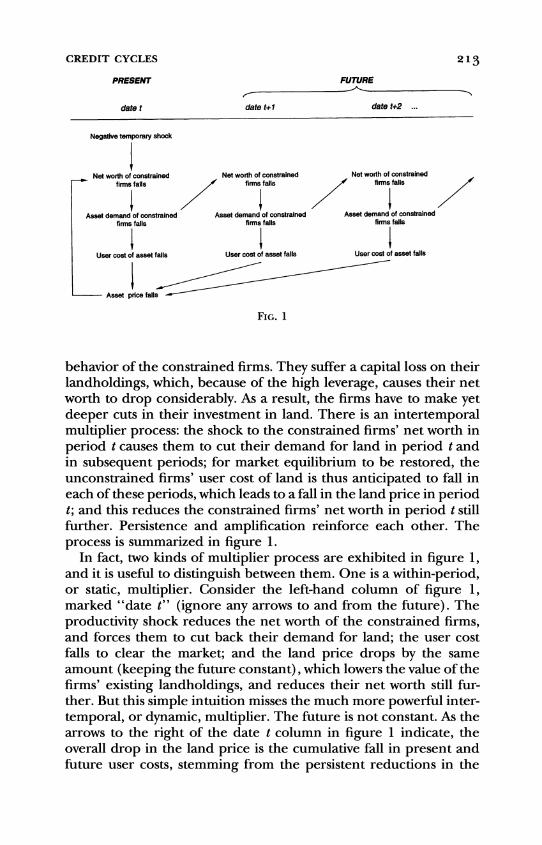
We select parameter values that might accord with a quarterly model: R = 1.01, equivalent to a 4 percent annual real interest rate; X = .975, equivalent to a 10 percent annual depreciation rate of trees; and u(K) K - v, where the intercept v is set to make 1l, the elasticity of the residual supply of land to farmers, equal to 10 percent in the steady state. Normalizing a = 1, we choose Kso that, in the steady state, the farmers use two-thirds of the total land stock. Let nt = 0.1; that is, the average interval between investments for a farmer is 2.5 years.
Define the aggregate debt/asset ratio as B1 [ (qt + 4)Kj] for the entire farming sector; and define the marginal debt/asset ratio as qt+l/ [R(qt + 0)], for a farmer who is investing in period t. We set 0 = 20, so that the steady-state values of these debt/asset ratios are 63 percent and 71 percent, respectively.
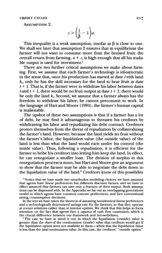
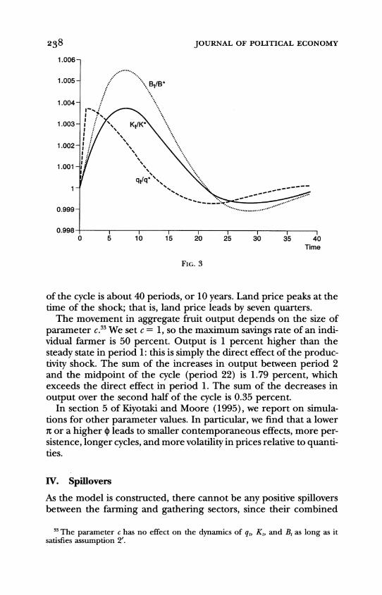
Consider an unanticipated, temporary productivity shock A = 0.01 in period 1. That is, there is a 1 percent increase in quarterly output of all the farmers and gatherers. Prior to the shock, the economy is in the steady state. In figure 3 we present the simulation results for qt/q*, K,/K*, and Bt/B*-the ratios of the land price, the farmers' aggregate landholding, and their aggregate debt to their respective steady-state values.
The contemporaneous effect of the shock is to increase the land price by 0.37 percent, and the farmers' landholding and debt by 0.10 percent and 0.13 percent. A 0.37 percent increase in the land price may not appear large, but it is much larger than it would be in a standard competitive model without credit constraints.32 The effects on the farmers' landholding and debt build up thereafter. By period 7 they peak, at 0.37 percent and 0.55 percent. The length
3' The algorithm is first to use (12), (23), and (24) to solve for (K,, B,, q,+,) as a function of (K,-,, B,-,, q,). Then we iterate to give the mapping from q, to qt+T.
Finally, we find the value of q, such that q,+T = q* for large T. We are thus able to confirm that the linear approximations are reasonably accurate. See Kiyotaki and Moore (1995, sec. 5) for details.
32 Recall that in a standard competitive model, the period 1 land price would not increase at all, because the shock does not affect the future. Alternatively, one might consider the possibility that, although the shock is announced in period 1, it will not happen until period 2-in which case the period 1 land price would increase only in the order of the net real interest rate, 0.01 percent.
238 JOURNAL OF POLITICAL ECONOMY
1.006-
1.005- .
1 .004-
1 .003 X-
1.001-1/A
f ~~~~~qlt/q "*
0.998- l 0 5 10 15 20 25 30 35 40
Time
FIG. 3
of the cycle is about 40 periods, or 10 years. Land price peaks at the time of the shock; that is, land price leads by seven quarters.
The movement in aggregate fruit output depends on the size of parameter C.33 We set c = 1, so the maximum savings rate of an indi- vidual farmer is 50 percent. Output is 1 percent higher than the steady state in period 1: this is simply the direct effect of the produc- tivity shock. The sum of the increases in output between period 2 and the midpoint of the cycle (period 22) is 1.79 percent, which exceeds the direct effect in period 1. The sum of the decreases in output over the second half of the cycle is 0.35 percent.
In section 5 of Kiyotaki and Moore (1995), we report on simula- tions for other parameter values. In particular, we find that a lower X or a higher ( leads to smaller contemporaneous effects, more per- sistence, longer cycles, and more volatility in prices relative to quanti- ties.
IV. Spillovers
As the model is constructed, there cannot be any positive spillovers between the farming and gathering sectors, since their combined
3 The parameter c has no effect on the dynamics of qt, Kt, and B, as long as it satisfies assumption 2'.
CREDIT CYCLES 239
land usage must always sum to K. In order to study spillover effects, we make an extension to the basic model of Section II so that it has two farming sectors, 1 and 2.
Suppose that there are different types of fruit. Gatherers make regular fruit, with the same production function as before. Farmers, however, produce slightly differentiated fruit. The farming technol- ogy is very similar to that in Section II. In sector i = 1 or 2, a farmer with land kit l at date t - 1 produces aiki,_l tradable fruit at date t, together with ciki,_l nontradable fruit. The only difference is that the tradable fruit is peculiar to that sector. The nontradable fruit is equivalent to regular fruit in consumption value to the farmer.
We assume that consuming a bundle comprising xj, fruit from sec- tor 1 and x21 fruit from sector 2 is equivalent to consuming x, regular fruit, where x1-E = xl-TE + x-'E. The parameter E > 0 is the inverse of the elasticity of substitution in consumption between the two types of fruit. We take E to be small: any positive value will pin down the size of each farming sector in equilibrium, and ensure that neither sector disappears.34
Let regular fruit be the numeraire good. Then at date t, the com- petitive price, pit say, of fruit from farming sector i is equal to the marginal rate of substitution:
Pit (ai Kiti-)-E[(a, Kjti)l- + (a2K2t-)lE]E/(lIe) fori= 1, 2 (31)
where Kit-, denotes the aggregate landholding of the farmers in sec- tor i at date t - 1.
As in (9), the aggregate landholding of the farmers in sector i at date t is given by
Kit= [(aipit + qt)Kitl - RBit-1] for i = 1, 2, (32)
qt - qt+l
where Bit-, denotes their aggregate debt at date t - 1. (The only substantive difference between [32] and [9] is that the tradable fruit output aiKit-1 is priced at pit rather than at unity.) And as in (10), the aggregate debt of the farmers in sector i at date t is given by
Bit = - qt+l Kit for i = 1, 2. (33) R
34 If the products of the two farming sectors were perfect substitutes (E = 0), then the sector with the higher productivity would eventually take over the whole mar- ket-unless a, = a2, in which case the sizes of the sectors would be indeterminate.
240 JOURNAL OF POLITICAL ECONOMY
The land market equilibrium condition is the same as (12), except that the farmers' landholdings from the two sectors are added to- gether:
qt - qt+l = u(Klt + K2t)* (34)
For given levels of Kit-, and Bi,-,, i = 1, 2, an equilibrium from date t onward is characterized by a sequence { (qt+, Pi,+,x Ki, s Bit+s)
Is - 0, i = 1, 2) satisfying equations (31), (32), (33), and (34) at datest,t+ 1,t+2,....35
Let us consider the impulse response to a sector-specific technol- ogy shock. Suppose that the economy is in the steady state at date t - 1, and, for simplicity, suppose that a, = a2 = a. As the two farm- ing sectors are symmetric, the steady state is described by (13) with K* = K* = K*/2 and B * = B * = B*/2. At the startofdate tthere is an unanticipated, temporary increase in the output of sector 1 only: the harvest of the farmers in sector 1 is 1 + A times the expected levels.
We can follow the argument of Section II to show that, for a small shock A, the proportional changes in the land price, qt, and the farm- ers' combined landholdings, Kjt + K2t, are half those given by (17) and (18), respectively-simply because only half of the farmers ex- perience the shock.
Our main concern is to see how the effects of the sector-specific shock are divided across the sectors:
Kjt= 1 + 1 _ lA (35a) 2(R - 1)(1 + T) 2
and
K2t L + ?]A. (35b) -2 (R -1) (1 + a) 2_
The first term in the brackets in (35a) is the direct impact of the productivity shock on the farmers in sector 1. However, given R close to one, this first term is dwarfed by the second term, the indirect effect on the farmers' land demand arising from the change in their
35 We continue to make assumptions 1 and 3 and a suitably modified version of assumption 2:
ci > 2/ (1 E)( - I) ai for i = 1, 2.
(The factor 2E/(1E-) here is the steady-state value of pi,, in the symmetric case a, = a2.)
CREDIT CYCLES 241
net worth caused by the jump in the land price. But this indirect benefit is enjoyed by the farmers in the other sector: (35b) is almost as large as (35a). In other words, because all the farmers hold land, the immediate spillover effect is significantly positive. (The E/2 terms in [35] represent demand linkage: expansion in sector 1 is partially offset by a fall in product price plt, which boosts sector 2's demand and product price P2t-)
Thereafter, the changes in the farmers' landholdings in each of the sectors follow the two-sector analogue of (15b): for s ' 1,
_ 1 _E 1~ +E
(K2t+s _ (_ ' 1- I _ ' t+s-1
2(1 +1q) 2 2(1 +1q) 2
Here the -1/2(1 + Tl) terms reflect the choking-off effect we identi- fied in Section II. That is, an increase in the demand for land by either farming sector causes the market-clearing user cost of land to rise, which partially chokes off demand in both sectors. This leads to a negative spillover between sectors after date t: for small E (negli- gible demand linkage), the off-diagonal entries in the transition ma- trix in (36) are negative. Crucially, however, the diagonal entries are positive-reflecting the fact that an increase in the landholdings of a farming sector at date t + s - 1 increases those farmers' net worth, and hence their land demand, at date t + s. Overall, the implication of (36) is that the initial increases Klt and K2t persist; and the two sectors comove after a shock, at least for a time.36
V. Related Literature and Final Remarks
The ideas in this paper can be traced at least as far back as Veblen (1904, chap. 5), who described the positive interactions between asset prices and collateralized borrowing. Since the theoretical litera- ture on financial structure and aggregate economic activity is vast, it would be unwise to attempt to review it here. We have picked out for discussion two papers that directly relate to our ideas.37
Bernanke and Gertler (1989) construct an overlapping genera- tions model in which financial market imperfections cause tempo-
6 The eigenvalues of the transition matrix in (36) are 1/ (1 + 11) and 1 - E, which both lie between zero and one.
3 For more on related papers, see Kiyotaki and Moore (1995). Gertler (1988) has written an excellent survey that not only identifies and clarifies the broader issues, but also provides an account of the historical developments.
242 JOURNAL OF POLITICAL ECONOMY
rary shocks in net worth to be amplified and to persist.38 All agents earn a wage when young, which they then invest for their old age. Some agents-entrepreneurs-have access to projects, which re- quire outside finance over and above the inside finance their own labor income provides. Because project returns can be verified only at a cost, financial contracts are imperfect, and so only a limited number of the better projects are funded. The projects that do go ahead provide employment for the next generation of young agents. In this economy, a positive technology shock both increases the la- bor demanded by the entrepreneurs who have been funded, and allows for more projects to be undertaken. Moreover, the accompa- nying rise in wage improves the financial position of the next genera- tion of entrepreneurs, so more of their projects will be funded too, they will subsequently demand more labor, and so on.
Aside from matters of modeling strategy,39 our model adds quite a kick to the Bernanke and Gertler story. At business cycle frequen- cies, a major channel for shocks to net worth is through changes in the values of firms' assets or liabilities. Asset prices reflect future market conditions. When the effects of a shock persist (as they do in Bernanke and Gertler), the cumulative impact on asset prices, and hence on net worth at the time of the shock, can be significant. This positive feedback through asset prices, and the associated inter- temporal multiplier process, are the key innovations in our paper.
The two-way feedback between borrowing limits and the price of assets connects with the paper by Shleifer and Vishny (1992) on debt capacity. They argue that when a firm in financial distress liquidates assets, the natural purchasers are other firms in the same industry. But if one firm is experiencing hard times, it is likely that other firms in the industry will be too, and so demand for liquidated assets will be lower. The concomitant fall in asset price exacerbates the prob- lem by lowering the debt capacity of all the firms. The essentially static nature of this argument-which is akin to the static multiplier process we identified in the Introduction-misses the more impor- tant dynamic multiplier process, and the crucial interplay between amplification and persistence. '
38 Greenwald and Stiglitz have pursued a similar line of inquiry; see, e.g., their 1993 paper.
39 We think that a model of debt that is based on control over assets, rather than on the cost of verifying project returns, is more compelling (and considerably simpler, especially when extended to more than two periods; see Gertler [1992]). For a com- parison of these two approaches, see the appendix to chap. 5 of Hart (1995).
4 A similar remark can be made with regard to the two-period multiple equilib- rium models of Kashyap, Scharfstein, and Weil (1990) and Lamont (1995).
We should mention two other papers that relate to ours. Stein (1995) analyzes trading in the housing market and shows that, because of leverage, an increase in the price of housing can increase net worth by more than the required down pay-
CREDIT CYCLES 243
There is some empirical evidence to support the view that invest- ment decisions are not solely determined by the net present value of new projects, but are also affected by an investing firm's balance sheet position and the value of its collateralized assets (see, e.g., Faz- zari, Hubbard, and Petersen 1988; Evans andJovanovic 1989; Hoshi, Kashyap, and Scharfstein 1991; Hubbard and Kashyap 1992; Whited 1992; Gertler and Gilchrist 1994; Holtz-Eakin, Joulfaian, and Rosen 1994; Gilchrist and Himmelberg 1995; Black, de Meza, and Jeffreys 1996). At the aggregate level, a number of studies have highlighted the importance of credit constraints in explaining fluctuations in activity; see in particular Bernanke (1983), Eckstein and Sinai (1986), and Friedman (1986).
The pressing next step in the research is to construct a fully fledged stochastic model, in which a shock is not a zero probability event and is rationally anticipated. In the paper we constructed a model of a dynamic economy that, at the aggregate level, is deter- ministic; and we then hit the economy with an unexpected tempo- rary shock. Although this approach succeeds in keeping the analysis tractable, it skirts around some central issues. The key question is, To what extent can contingent debt contracts be written? There are a number of explanations for why it may be impossible to condition debt repayments on idiosyncratic shocks. For example, such shocks may not be observable to outsiders, such as the courts (see Hart and Moore 1996).4 However, it is less clear why the terms of a contract cannot be made sensitive to aggregate events, such as movements in the price of land or in the interest rate. This is a difficult matter to resolve.
Let us turn to less thorny issues. A weakness of our model is that it provides no analysis of who becomes credit constrained, and when. We merely rely on the assumption that different agents have differ- ent technologies. One can instead assume that all agents have access to a common, concave technology, but differ in their levels of accu- mulated wealth. Ortalo-Magne (1996) constructs a life cycle model
ment, leading to an increase in the demand for houses. That is, as in our model, asset demand schedules can slope upward. Although Stein's model is not dynamic, his paper provides an interesting explanation for the observed correlation between price and trading volume in the housing market.
Scheinkman and Weiss (1986) construct a dynamic general equilibrium model in which a durable, nonproduced asset serves as a means for precautionary saving. In their model, only the net positions of agents matter: there are no leverage effects. By contrast, in our model the asset provides security for borrowing. And because an agent needs the asset in order to produce, he holds a levered position-which make his net worth very vulnerable to changes in the asset price.
41 Even if financial contracts can be written contingent on idiosyncratic shocks, it may not be efficient to diversify risk fully, for standard moral hazard reasons.
244 JOURNAL OF POLITICAL ECONOMY
of farming and agricultural land prices. Farmers borrow against their landholdings, and are most likely to face borrowing constraints when they are young and relatively poor. As they save and accumulate assets, they become unconstrained.42
Finally, it would be interesting to relax the assumption that, on the supply side, the credit market is anonymous. In the paper we have implicitly taken the position that debt contracts can be freely traded by creditors-because the value of a debt contract equals the value of the collateral, land, which is priced in a market. However, the identity of the creditor may matter. A particular creditor may have additional information about, or leverage over, a particular bor- rower, which enables the creditor to lend more. Such debt contracts are unlikely to be tradable at full value. Once anonymity is dropped, the net worth of creditors, and the value of their collateral, start to matter. The interaction between asset markets and credit markets that we have highlighted in this paper will be even richer if both sides of the credit market are affected by changes in the price of their collateralized assets.
Appendix
This appendix sketches an overlapping generations version of the basic model of Section II. The main purpose is to show that our two unorthodox modeling choices-the assumption that agents have linear preferences but different discount factors, and the assumption that a fraction of the farmers' output is nontradable-can both be dispensed with in an overlapping gen- erations framework.
Consider an economy in which agents die with probability 1 - a between one date and the next, and survive with probability (. Death is independent across agents (there is no aggregate uncertainty), and independent of an agent's age, technology, or net worth. The total population has mea- sure 1 + m, and comprises farmers and gatherers in ratio 1: m. At each date, new farmers and gatherers are born, with populations 1 - a and (1 - a) m. Newborns are endowed with a small amount, e, of fruit per unit of population.
All fruit is tradable. At each date t, agents maximize the expected dis- counted utility of fruit consumption, x,,,, conditional on surviving to date t+ s:
E[Z (o) s In xt+s,
42 Firms may well go through similar kinds of life cycles. An alternative to the overlapping generations framework would be to assume that agents face a stochastic technology, as in Scheinkman and Weiss (1986).
CREDIT CYCLES 245
where fB E (0, 1) is their common discount factor, and In x, the natural logarithm of x, is their common utility function.
Farmers and gatherers differ only in their technologies. If a farmer invests in k, land at date t and survives to date t + 1, then, unless he withdraws his labor, he produces akt fruit. By contrast, a gatherer cannot withdraw his labor during production: if he invests in k' land at date t and survives to date t + 1, then he produces G(k') fruit, per unit of population, where G' > 0, G" < 0, and G'(O) > a > sa > G'(K/m). (These last inequalities ensure that in the neighborhood of the steady state, both farmers and gath- erers produce.) If an agent dies, there is no fruit output, but the land re- mains. In what follows, we ignore unanticipated productivity shocks, and just consider perfect-foresight paths.
There is no bequest motive, and so all agents will choose to mortgage their land fully at each date t, by borrowing up to the collateral value. That is, they pay only the down payment
1 Ut = qt - - qt+l (Al)
Rt
on land, where Rt is the gross rate of interest on debt. In addition, gatherers may choose to borrow against some or all of their
fruit output, since they cannot threaten to withdraw# their labor. To this end, an individual gatherer may issue an "annuity" contract: in return for borrowing one unit of fruit at date t, he promises to repay Rt/o fruit at date t + 1 if he survives until then. (The only constraint here is that no gatherer can issue more annuities than can be repaid out of his date t + 1 fruit output, G(k). In the neighborhood of the steady state, this con- straint does not bind.) A wealthy (old) gatherer may choose to buy annui- ties; that is, pay one unit of fruit at date t in order to receive Rt/o fruit at date t + 1 if he survives. Because there is no aggregate uncertainty, the fraction of gatherers who survive is exactly a; and so, through pooling, no one need be exposed to anyone else's risk.
Farmers cannot precommit not to withdraw their labor, and so cannot credibly issue annuities. Moreover, they will not choose to buy annuities, provided that the return on farming is greater:
I-a >-IRat (A2) 1t a
We shall show later that (A2) holds in the neighborhood of the steady state. Since a fraction 1 - a of the farmers die between dates t - 1 and t, since
all land is mortgaged, and since no farmer buys annuities, the net worth of the farmers alive at date t equals the surviving farmers' output 0aKt-I (where K,_1 is the aggregate landholding of farmers at the end of date t - 1) plus the newborn farmers' endowment (1 - ) e. Given logarithmic preferences, farmers spend a fixed proportion, 1 -Po, of their net worth on consumption. The rest is used as a down payment on land:
Kt= -I [oaKtl + (1 - 0)e]. (A3) Ut
246 JOURNAL OF POLITICAL ECONOMY
Gatherers also spend a fixed proportion 1 - jB of their net worth on consumption. Aggregating across farmers and gatherers, we can equate consumption demand at date t to total fruit output, Yt:
(1 - Po) (Yt + qtK+ mVt) = t, (A4)
where the term in the second set of parentheses is the aggregate net worth of the current population, and Vt is the net worth of a gatherer's technology:
Vt = 2 G(kt) - utk + - Vt+1. (A5) Rt t Rt
Here k' equates the marginal return on gathering to that on annuities:
G'(kt) --Rt. (A6) Ut 0
The land market clears:
Kt + mk' = K. (A7)
Total fruit output comprises the output of the surviving farmers and gath- erers, plus the endowment of the newborn:
Yt = oaKt-I + cYmG[ (K- Ktl)1 + (1 + m)(I + o)e. (A8)
In a stable equilibrium, equations (Al) and (A3) - (A8) hold at each date t, subject to condition (A2), and the expected discounted values of qt+s and Vt+, converge to zero as s tends to infinity.
Denote steady-state values with an asterisk. It is straightforward to show the following proposition.
PROPOSITION. For small e, there is a unique steady-state equilibrium in which the farmers' credit constraints are binding.43 The equilibrium R* lies strictly between 1 / j3 and 1 / Pa.
To confirm that condition (A2) is satisfied, notice from (A3) that if the size of the farming sector is to stay constant in the steady state, then u* must equal approximately fk&2a (for small e). Thus, in the neighborhood of the steady state, (A2) reduces to R* < 1/ Pa.
There are two important points to observe. First, an individual farmer grows if he survives, because his savings rate times his return on land, jaa, exceeds the down payment, uO. However, in aggregate the net worth of the farming sector does not grow because as rich old farmers die they are re- placed by poor young ones.
Second, R* > 1/ P implies that the return on annuities, R* / a, exceeds the effective rate of time preference, 1/ jo. Hence a gatherer chooses an upward-sloping path of lifetime consumption, which is the source of loan- able funds in the economy.
Details of how this overlapping generations economy responds to an un-
43 There is no steady-state equilibrium in which the farmers' credit constraints are not binding.
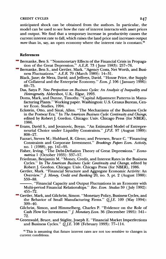
CREDIT CYCLES 247
anticipated shock can be obtained from the authors. In particular, the model can be used to see how the rate of interest interacts with asset prices and output. We find that a temporary increase in productivity causes the current interest rate to fall, which raises the land price and increases output more than in, say, an open economy where the interest rate is constant.44
References
Bernanke, Ben S. "Nonmonetary Effects of the Financial Crisis in Propaga- tion of the Great Depression." A.E.R. 73 (June 1983): 257-76.
Bernanke, Ben S., and Gertler, Mark. "Agency Costs, Net Worth, and Busi- ness Fluctuations." A.E.R 79 (March 1989): 14-31.
Black, Jane; de Meza, David; and Jeffreys, David. "House Price, the Supply of Collateral and the Enterprise Economy." Econ. J. 106 (January 1996): 60-75.
Das, Satya P. New Perspectives on Business Cycles: An Analysis of Inequality and Heterogeneity. Aldershot, U.K: Elgar, 1993.
Doms, Mark, and Dunne, Timothy. "Capital Adjustment Patterns in Manu- facturing Plants." Working paper. Washington: U.S. Census Bureau, Cen- ter Econ. Studies, 1994.
Eckstein, Otto, and Sinai, Allen. "The Mechanisms of the Business Cycle in the Postwar Era." In The American Business Cycle: Continuity and Change, edited by Robert J. Gordon. Chicago: Univ. Chicago Press (for NBER), 1986.
Evans, David S., and Jovanovic, Boyan. "An Estimated Model of Entrepre- neurial Choice under Liquidity Constraints." JP.E. 97 (August 1989): 808-27.
Fazzari, Steven M.; Hubbard, R. Glenn; and Petersen, Bruce C. "Financing Constraints and Corporate Investment." Brookings Papers Econ. Activity, no. 1 (1988), pp. 141-95.
Fisher, Irving. "The Debt-Deflation Theory of Great Depressions." Econo- metrica 1 (October 1933): 337-57.
Friedman, Benjamin M. "Money, Credit, and Interest Rates in the Business Cycles." In The American Business Cycle: Continuity and Change, edited by RobertJ. Gordon. Chicago: Univ. Chicago Press (for NBER), 1986.
Gertler, Mark. "Financial Structure and Aggregate Economic Activity: An Overview." J Money, Credit and Banking 20, no. 3, pt. 2 (August 1988): 559-88.
. "Financial Capacity and Output Fluctuations in an Economy with Multi-period Financial Relationships." Rev. Econ. Studies 59 (July 1992): 455-72.
Gertler, Mark, and Gilchrist, Simon'. "Monetary Policy, Business Cycles, and the Behavior of Small Manufacturing Firms." QJE. 109 (May 1994): 309-40.
Gilchrist, Simon, and Himmelberg, Charles P. "Evidence on the Role of Cash Flow for Investment." J. Monetary Econ. 36 (December 1995): 541- 72.
Greenwald, Bruce, and Stiglitz, Joseph E. "Financial Market Imperfections and Business Cycles." Q.J.E. 108 (February 1993): 77-114.
4 This is assuming that future interest rates are not too sensitive to changes in current conditions.
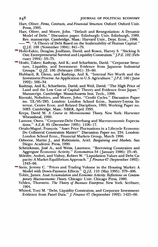
248 JOURNAL OF POLITICAL ECONOMY
Hart, Oliver. Firms, Contracts, and Financial Structure. Oxford: Oxford Univ. Press, 1995.
Hart, Oliver, and Moore, John. "Default and Renegotiation: A Dynamic Model of Debt." Discussion paper. Edinburgh: Univ. Edinburgh, 1989. Rev. manuscript. Cambridge, Mass.: Harvard Univ., Dept. Econ., 1996.
. "A Theory of Debt Based on the Inalienability of Human Capital." QJE. 109 (November 1994): 841-79.
Holtz-Eakin, Douglas; Joulfaian, David; and Rosen, Harvey S. "Sticking It Out: Entrepreneurial Survival and Liquidity Constraints."JP.E. 102 (Feb- ruary 1994): 53-75.
Hoshi, Takeo; Kashyap, Anil K; and Scharfstein, David. "Corporate Struc- ture, Liquidity, and Investment: Evidence from Japanese Industrial Groups." QJE. 106 (February 1991): 33-60.
Hubbard, R. Glenn, and Kashyap, Anil K "Internal Net Worth and the Investment Process: An Application to U.S. Agriculture."J.P.E. 100 (June 1992): 506-34.
Kashyap, Anil K; Scharfstein, David; and Weil, David. "The High Price of Land and the Low Cost of Capital: Theory and Evidence from Japan." Manuscript. Cambridge: Massachusetts Inst. Tech., 1990.
Kiyotaki, Nobuhiro, and Moore, John. "Credit Cycles." Discussion Paper no. TE/95/285. London: London School Econ., Suntory-Toyota In- ternat. Centre Econ. and Related Disciplines, 1995; Working Paper no. 5083. Cambridge, Mass.: NBER, April 1995.
Kreps, David M. A Course in Microeconomic Theory. New York: Harvester Wheatsheaf, 1990.
Lamont, Owen. "Corporate-Debt Overhang and Macroeconomic Expecta- tions." A.E.R. 85 (December 1995): 1106-17.
Ortalo-Magne' Franscois. "Asset Price Fluctuations in a Lifecycle Economy: Do Collateral Constraints Matter?" Discussion Paper no. 234. London: London School Econ., Financial Markets Group, March 1996.
Osborne, Martin J., and Rubinstein, Ariel. Bargaining and Markets. San Diego: Academic Press, 1990.
Scheinkman, Jose A., and Weiss, Laurence. "Borrowing Constraints and Aggregate Economic Activity." Econometrica 54 (January 1986): 23-45.
Shleifer, Andrei, and Vishny, Robert W. "Liquidation Values and Debt Ca- pacity: A Market Equilibrium Approach."J Finance 47 (September 1992): 1343-66.
Stein, Jeremy C. "Prices and Trading Volume in the Housing Market: A Model with Down-Payment Effects." Q.JE. 110 (May 1995): 379-406.
Tobin, James. Asset Accumulation and Economic Activity: Reflections on Contem- porary Macroeconomic Theory. Chicago: Univ. Chicago Press, 1980.
Veblen, Thorstein. The Theory of Business Enterprise. New York: Scribner, 1904.
Whited, Toni M. "Debt, Liquidity Constraints, and Corporate Investment: Evidence from Panel Data." J Finance 47 (September 1992): 1425-60.