Automated input attribute weighting for unsupervised seismic facies analysis Tao Zhao*, Fangyu Li, and Kurt J. Marfurt, University of Oklahoma

SUMMARY

Typically, interpreters qualitatively choose input attributes for multiattribute facies analysis based on their experience and geologic target of interest. In this study, we augment this qualitative attribute selection process with quantitative measures of which candidate attributes best differentiate features of interest, by weighting input attributes based on their response from the unsupervised learning algorithm that used to generate the facies map, as well as interpreter’s preference. We use self-organizing map (SOM) as an example of unsupervised seismic facies analysis algorithm. By comparing with results from equally weighted attributes, we demonstrate that the proposed attribute weighting workflow is able to represent the information from the input attributes more adequately.

INTRODUCTION

With the rapid development in seismic attribute and interpretation techniques, interpreters can be overwhelmed by the number of attributes available at their disposal. Barnes (2007) discusses redundant attributes, stating that there are many duplicate attributes, and many attributes with vague geological meaning. Excluding those redundant attributes greatly simplifies the seismic interpretation workflow. However, interpreters still face the challenge of selecting which of the remaining attributes are appropriate for a given interpretation task.

Researchers have spent considerable amount of effort on how to qualitatively and quantitatively select the most suitable attributes for facies and reservoir property estimation. Chen and Sidney (1997) provide a comprehensive review of attribute selection for reservoir predicting and monitoring. Kalkomey (1997) discusses the risk of false correlation between seismic attributes and reservoir properties, in which she suggests that special caution is needed when there are few wells to correlate or using too many attributes. Hart and Balch (2000) present a case study on predicting reservoir properties from seismic attributes with limited well control, and propose a suite of visual correlation schemes to define the attributes of choice. From a more quantitative aspect, Schuelke and Quirein (1998) propose to use cross-validation as a measure of prediction performance, then select attributes that lead to higher cross-validation. Since then, almost all the proposed alternative strategies have shared one fundamental concept, which is to select attributes that lead to the lowest validation error. One example is from Dorrington and Link (2004), in which the authors use a genetic algorithm (a popular

nonlinear inversion approach) to automatically determine input attributes based on the error of a neural network porosity prediction.

Such prediction error based approaches are of great value if the facies analysis is in a supervised fashion, which means the interpreters provide training data to the learning algorithm. In scenarios that no training data are available and the objective is to discover natural facies distribution in the data, interpreters use unsupervised learning algorithms, such as self-organizing map (SOM), to cluster the multiattribute input data. In Barnes and Laughlin (2002), the authors conclude that the selection of input attributes has a higher impact on the facies map than the unsupervised learning algorithm used for classification. Qualitatively, Zhao et al. (2015) review several competing unsupervised learning algorithms and provide a recommendation of attributes to highlight different architectural elements in a turbidite system. By using principal component analysis (PCA), Roden et al. (2015) determine the amount of variation contributed from each seismic attribute to the top principal components of a large number of attributes, then select the attributes with the highest contribution to be used in the subsequent facies analysis. Although PCA estimates the contribution of each attribute to represent the data variability as a whole, it does not provide a measure of attribute importance to the subsequence unsupervised learning process.

The attribute selection system we use today is in fact simply a weighting system: if we use an attribute, its weight is one; if we reject it, its weight is zero. We therefore propose to use a weighting scheme that instead of either selecting or rejecting an attribute, we define weights that represent the value of each input attribute in differentiating facies of interest. We weight the interpreter-selected input attributes base on both their response from the unsupervised learning algorithm and interpreter’s knowledge. The weights therefore represent both “which attribute is favored by an interpreter as input for unsupervised learning” from an interpretation perspective, and “which attribute is ‘favored’ by the learning algorithm” from a data-driven perspective. We use SOM as the example of the unsupervised learning algorithm, and provide the definition of attribute weights in the next section.

DEFINITION OF ATTRIBUTE WEIGHTS

To emphasize and deemphasize the importance of a given attribute, we define a weight matrix W when calculating distance in SOM:

© 2017 SEG SEG International Exposition and 87th Annual Meeting

Page 2122

Dow

nloa

ded

02/0

9/18

to 1

29.1

5.66

.178

. Red

istr

ibut

ion

subj

ect t

o SE

G li

cens

e or

cop

yrig

ht; s

ee T

erm

s of

Use

at h

ttp://

libra

ry.s

eg.o

rg/

Attribute weighting in facies analysis

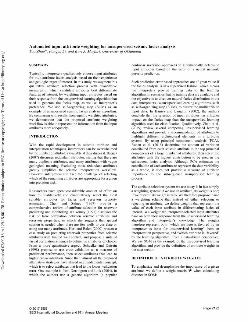
𝑟 = (𝐚1 ‒ 𝐚2)𝑇𝐖(𝐚1 ‒ 𝐚2). (1)Here, and are two z-score normalized 𝐚1 𝐚2 𝑁⨯1multiattribute data vectors of N attributes, r is the distance between the two multiattribute data vectors, and W is a diagonal matrix. We show a schematic plot of two attributes in Figure 1 to demonstrate the effect of the distance matrix W on data clustering.

Figure 1. A schematic drawing to show the effect of weighting attributes. (a) Two equally weighted attributes with three clusters. The red and green clusters are very close such that a distance-based clustering algorithm may only find two instead of three clusters. (b) The same data samples but now with different weights applied to the two attributes changing their distance from the origin. The red and green clusters are now better separated.

Inspired by Benabdeslem and Lebbah (2007), given N input attributes and J prototype vectors (which are the proxies of the 2D SOM neurons in the attribute space), we define , 𝜔𝑖the ith attribute’s contribution to a SOM model, as:

𝜔𝑖 =𝐽

∑𝑗 = 1

𝑑𝑗

|𝑝𝑗𝑖|𝑁

∑𝑘 = 1

|𝑝𝑗𝑘|, (2)

and

𝑑𝑗 =ℎ𝑗

𝑀, (3)

where hj is the number of multiattribute training samples that are nearest to the jth prototype vector, M is the total number of multiattribute training samples, dj represents the density of training samples assigned to the jth prototype vectors, and pjk is the value of the jth prototype vector along dimension k (the dimension of the kth attribute). Physically, if a prototype vector has a very large value in the dimension of the target attribute, and a large percentage of training samples are close to this prototype vector, then the target attribute’s contribution at this prototype vector is significant. Summing up over all the prototype vectors, we then arrive at the target attribute’s contribution to the whole SOM model.

We loosely define an “edge” attribute to be an attribute representing the variation among neighboring seismic samples, and a “body” attribute to be an attribute representing a property of a seismic sample or samples within a window. And for seismic facies analysis, we prefer

body attributes with color representation so that the edge information becomes complimentary. A body attribute has a flatter and more symmetric histogram, whereas an edge attribute’s histogram is tighter and skewed. Therefore, we propose to use skewness s, and kurtosis, k, which measures the symmetry and sharpness of a histogram, to quantify the interpreter’s preference of body attributes over edge attributes. We finally define an element in the weight matrix W to be:

𝑊𝑖𝑖 =2

1 + 𝑒‒ 𝑤𝑖

, (4)

where is the weight for the ith attribute, and is a 𝑊𝑖𝑖 𝑤𝑖function of , , and . Once we compute the weight 𝜔𝑖 𝑠𝑖 𝑘𝑖matrix W, we use the distance representation in equation 1 in the SOM algorithm so that different attributes are emphasized accordingly to their weight values.

APPLICATION

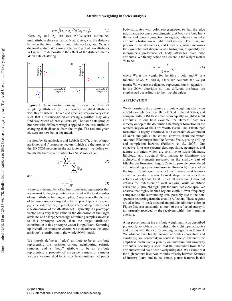
We demonstrate the proposed attribute weighting scheme on a field example from the Barnett Shale, United States, and compare with SOM facies map from equally weighted input attributes. In our field example, the Barnett Shale lies directly on top of the dolomitic Ellenburger formation in the western region of the Fort Worth Basin. The Ellenburger formation is highly deformed, with extensive development of karst and joints that extend upwards from the water-saturated Ellenburger into the Barnett Shale, posing drilling and completion hazards (Pollastro et al., 2007). Our objective is to use spectral decomposition, geometric, and texture attributes, which are sensitive to strata thickness, lithology, and structural deformation, to illuminate the architectural elements presented in the shallow part of Ellenburger formation. Figure 2a to 2d provide co-rendered attributes along a phantom horizon (Horizon A) 25 ms below the top of Ellenburger, on which we observe karst features either in isolated circular to oval shape, or in a cellular network of polygonal karst. Structural curvature (Figure 2a) defines the extension of karst regions, while amplitude curvature (Figure 2b) highlights the small scale collapse. We observe that highly karsted regions exhibit lower frequency compared to the surrounding area, possibly due to the non-specular scattering from the chaotic reflectors. These regions are also low in peak spectral magnitude (dimmer color in Figure 2c), as a substantial amount of the reflected energy is not properly received by the receivers within the migration aperture.

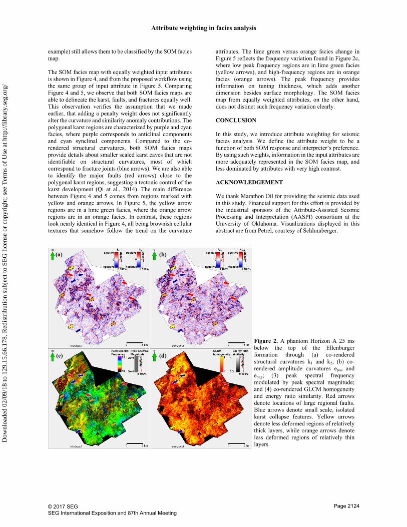
After precomputing the attribute weight matrix as described previously, we obtain the weights of the eight input attributes and display with their corresponding histograms in Figure 3. We observe that highly skewed attributes (curvature and similarity) are penalized; in contrast, “body” attributes are amplified. With such a penalty on curvature and similarity attributes, one may suspect that the anomalies from these attributes would have been overly mitigated. We assume that the high contrast in curvature and similarity between features of interest (karst and faults, versus planar features in this

© 2017 SEG SEG International Exposition and 87th Annual Meeting

Page 2123

Dow

nloa

ded

02/0

9/18

to 1

29.1

5.66

.178

. Red

istr

ibut

ion

subj

ect t

o SE

G li

cens

e or

cop

yrig

ht; s

ee T

erm

s of

Use

at h

ttp://

libra

ry.s

eg.o

rg/

Attribute weighting in facies analysis

example) still allows them to be classified by the SOM facies map.

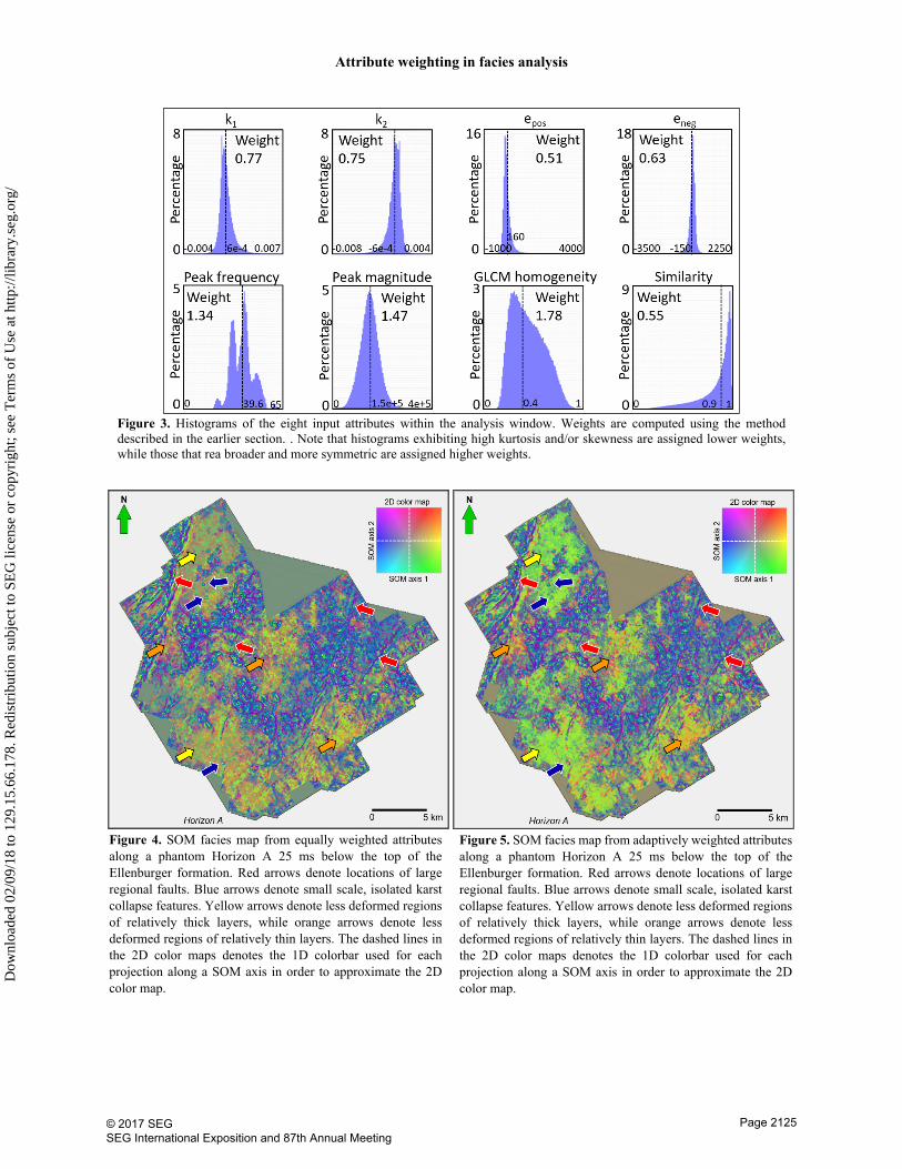
The SOM facies map with equally weighted input attributes is shown in Figure 4, and from the proposed workflow using the same group of input attribute in Figure 5. Comparing Figure 4 and 5, we observe that both SOM facies maps are able to delineate the karst, faults, and fractures equally well. This observation verifies the assumption that we made earlier, that adding a penalty weight does not significantly alter the curvature and similarity anomaly contributions. The polygonal karst regions are characterized by purple and cyan facies, where purple corresponds to anticlinal components and cyan synclinal components. Compared to the co-rendered structural curvatures, both SOM facies maps provide details about smaller scaled karst caves that are not identifiable on structural curvatures, most of which correspond to fracture joints (blue arrows). We are also able to identify the major faults (red arrows) close to the polygonal karst regions, suggesting a tectonic control of the karst development (Qi at al., 2014). The main difference between Figure 4 and 5 comes from regions marked with yellow and orange arrows. In Figure 5, the yellow arrow regions are in a lime green facies, where the orange arrow regions are in an orange facies. In contrast, these regions look nearly identical in Figure 4, all being brownish cellular textures that somehow follow the trend on the curvature

attributes. The lime green versus orange facies change in Figure 5 reflects the frequency variation found in Figure 2c, where low peak frequency regions are in lime green facies (yellow arrows), and high-frequency regions are in orange facies (orange arrows). The peak frequency provides information on tuning thickness, which adds another dimension besides surface morphology. The SOM facies map from equally weighted attributes, on the other hand, does not distinct such frequency variation clearly.

CONCLUSION

In this study, we introduce attribute weighting for seismic facies analysis. We define the attribute weight to be a function of both SOM response and interpreter’s preference. By using such weights, information in the input attributes are more adequately represented in the SOM facies map, and less dominated by attributes with very high contrast.

ACKNOWLEDGEMENT

We thank Marathon Oil for providing the seismic data used in this study. Financial support for this effort is provided by the industrial sponsors of the Attribute-Assisted Seismic Processing and Interpretation (AASPI) consortium at the University of Oklahoma. Visualizations displayed in this abstract are from Petrel, courtesy of Schlumberger.

(c) (d)

(a) (b)

Figure 2. A phantom Horizon A 25 ms below the top of the Ellenburger formation through (a) co-rendered structural curvatures k1 and k2; (b) co-rendered amplitude curvatures epos and eneg; (3) peak spectral frequency modulated by peak spectral magnitude; and (4) co-rendered GLCM homogeneity and energy ratio similarity. Red arrows denote locations of large regional faults. Blue arrows denote small scale, isolated karst collapse features. Yellow arrows denote less deformed regions of relatively thick layers, while orange arrows denote less deformed regions of relatively thin layers.

© 2017 SEG SEG International Exposition and 87th Annual Meeting

Page 2124

Dow

nloa

ded

02/0

9/18

to 1

29.1

5.66

.178

. Red

istr

ibut

ion

subj

ect t

o SE

G li

cens

e or

cop

yrig

ht; s

ee T

erm

s of

Use

at h

ttp://

libra

ry.s

eg.o

rg/

Attribute weighting in facies analysis

Figure 4. SOM facies map from equally weighted attributes along a phantom Horizon A 25 ms below the top of the Ellenburger formation. Red arrows denote locations of large regional faults. Blue arrows denote small scale, isolated karst collapse features. Yellow arrows denote less deformed regions of relatively thick layers, while orange arrows denote less deformed regions of relatively thin layers. The dashed lines in the 2D color maps denotes the 1D colorbar used for each projection along a SOM axis in order to approximate the 2D color map.

Figure 3. Histograms of the eight input attributes within the analysis window. Weights are computed using the method described in the earlier section. . Note that histograms exhibiting high kurtosis and/or skewness are assigned lower weights, while those that rea broader and more symmetric are assigned higher weights.

Figure 5. SOM facies map from adaptively weighted attributes along a phantom Horizon A 25 ms below the top of the Ellenburger formation. Red arrows denote locations of large regional faults. Blue arrows denote small scale, isolated karst collapse features. Yellow arrows denote less deformed regions of relatively thick layers, while orange arrows denote less deformed regions of relatively thin layers. The dashed lines in the 2D color maps denotes the 1D colorbar used for each projection along a SOM axis in order to approximate the 2D color map.

© 2017 SEG SEG International Exposition and 87th Annual Meeting

Page 2125

Dow

nloa

ded

02/0

9/18

to 1

29.1

5.66

.178

. Red

istr

ibut

ion

subj

ect t

o SE

G li

cens

e or

cop

yrig

ht; s

ee T

erm

s of

Use

at h

ttp://

libra

ry.s

eg.o

rg/

EDITED REFERENCES

Note: This reference list is a copyedited version of the reference list submitted by the author. Reference lists for the 2017

SEG Technical Program Expanded Abstracts have been copyedited so that references provided with the online

metadata for each paper will achieve a high degree of linking to cited sources that appear on the Web.

REFERENCES

Barnes, A. E., 2007, Redundant and useless seismic attributes: Geophysics, 72, no. 3, P33–P38,

http://doi.org/10.1190/1.2716717.

Barnes, A. E., and K. J. Laughlin, 2002, Investigation of methods for unsupervised classification of

seismic data: 72nd Annual International Meeting, SEG, Expanded Abstracts, 2221–2224,

http://doi.org/10.1190/1.1817152.

Benabdeslem, K., and M. Lebbah, 2007, Feature selection for self-organizing map: IEEE 29th

International Conference on Information Technology Interfaces, 45–50,

http://doi.org/10.1109/ITI.2007.4283742.

Chen, Q., and S. Sidney, 1997, Seismic attribute technology for reservoir forecasting and monitoring: The

Leading Edge, 16, 445–448, http://doi.org/10.1190/1.1437657.

Dorrington, K. P., and C. A. Link, 2004, Genetic-algorithm/neural-network approach to seismic attribute

selection for well-log prediction: Geophysics, 69, 212–221, http://doi.org/10.1190/1.1649389.

Hart, B. S., and R. S. Balch, 2000, Approaches to defining reservoir physical properties from 3-D seismic

attributes with limited well control: An example from the Jurassic Smackover Formation,

Alabama: Geophysics, 65, 368–376, http://doi.org/10.1190/1.1444732.

Kalkomey, C. T., 1997, Potential risks when using seismic attributes as predictors of reservoir properties:

The Leading Edge, 16, 247–251, http://doi.org/10.1190/1.1437610.

Pollastro, R. M., D. M. Jarvie, R. J. Hill, and C. W. Adams, 2007, Geologic framework of the

Mississippian Barnett shale, Barnett-paleozoic total petroleum system, Bend arch—Fort Worth

Basin, Texas: AAPG Bulletin, 91, 405–436, http://doi.org/10.1306/10300606008.

Qi, J., B. Zhang, H. Zhou, and K. Marfurt, 2014, Attribute expression of fault-controlled karst—Fort

Worth Basin, Texas: A tutorial: Interpretation, 2, SF91–SF110, http://doi.org/10.1190/INT-2013-

0188.1.

Roden, R., T. Smith, and D. Sacrey, 2015, Geologic pattern recognition from seismic attributes: Principal

component analysis and self-organizing maps: Interpretation, 4, SAE59–SAE83,

http://doi.org/10.1190/INT-2015-0227.1.

Schuelke, J. S., and J. A. Quirein, 1998, Validation: A technique for selecting seismic attributes and

verifying results: 68th Annual International Meeting, SEG, Expanded Abstracts, 936–939,

http://doi.org/10.1190/1.1820645.

Zhao, T., V. Jayaram, A. Roy, and K. J. Marfurt, 2015, A comparison of classification techniques for

seismic facies recognition: Interpretation, 3, SAE29–SAE58, http://doi.org/10.1190/INT-2015-

0044.1.

© 2017 SEG SEG International Exposition and 87th Annual Meeting

Page 2126

Dow

nloa

ded

02/0

9/18

to 1

29.1

5.66

.178

. Red

istr

ibut

ion

subj

ect t

o SE

G li

cens

e or

cop

yrig

ht; s

ee T

erm

s of

Use

at h

ttp://

libra

ry.s

eg.o

rg/