automatic adaptive finite element mesh generation over rational b-spline surfaces

Automatic adaptive ®nite element mesh generation overrational B-spline surfaces

C. K. Lee *, R. E. Hobbs

Department of Civil Engineering, Imperial College of Science, Technology and Medicine, London, SW7 2BU, U.K.

Received 9 October 1996; accepted 21 April 1998

Abstract

A new approach is suggested for the generation of adaptive ®nite element meshes over three-dimensional surfaces.

The surfaces to be meshed are represented as the unions of rational B-spline surface (RBSS) patches such that themesh generation process is reduced to the formation of nodes and elements in a parametric space. A robust andre®ned triangular element formation procedure is employed for the generation of highly skewed meshes in theparametric space such that well-shaped ®nite elements are obtained after mapping back to the three-dimensional

(3D) space. By carefully monitoring the geometrical distortion e�ect due to the parametric mapping, the suggestedelement formation procedure can be used on convoluted and rough surfaces without impairing the quality of themeshes generated. In fact, the proposed generation scheme can easily be extended to many other bivariate surfaces

without major modi®cation. A simple and e�ective conversion scheme is also developed for the generation of purequadrilateral meshes. Numerical experiments show that the operational complexity of the surface mesh generator isexactly the same as in two-dimensional (2D) planar mesh generation. High quality ®nite element meshes with

element size grading compatible with the speci®ed node spacing requirement are generated within a reasonable timelimit in a common small computing environment. # 1998 Elsevier Science Ltd. All rights reserved.

Keywords: Automatic surface mesh generation; Advancing front technique; Rational B-spline surfaces

1. Introduction

Recently, many advances have been made in the

development of a fully automatic ®nite element mesh

generator, particularly by using either the advancing

front technique (AFT) [1±3] or the recursive domain de-

composition method [4, 5]. It is generally accepted that

both of these approaches can be used for the gener-

ation of high quality graded meshes suitable for adap-

tive ®nite element analysis, at least for two-

dimensional (2D) problems [6±8].

The next step in the development of automatic mesh

generation schemes is the discretization of domains

consisting of non-planar surfaces. Several algorithms

have been suggested by extending existing 2D mesh

generation principles. Some early work involved map-

ping techniques similar to isoparametric element

mapping [9], the more general B-spline lofting [10] and

the curvilinear coordinate transformation

techniques [11]. In a more mature approach, the target

surface is ®rst represented by an assembly of bivariate

parametric surface patches. A 2D mesh generator is

then employed for the formation of elements in the

parametric space and the ®nal mesh obtained through

one or even two cycles of mapping [12]. Of course, for

mesh generation in the parametric space, either the

advancing front mesh generators [12] or the recursive

domain decomposition generators [13, 14] could be

used. The advantage of this generation plus mapping

approach is that by ®rst generating the ®nite element

mesh in the parametric space, the node and element

generation procedure will be reduced to a simple task

of planar mesh generation. However, one shortcoming

Computers and Structures 69 (1998) 577±608

0045-7949/98/$ - see front matter # 1998 Elsevier Science Ltd. All rights reserved.

PII: S0045-7949(97 )00106-0

PERGAMON

* Present address: School of Civil and Structural

Engineering, Nanyang Technological University, Nanyang

Avenue, Singapore 639798. E-mail: [email protected].

of this approach is that if the distortion e�ects induced

by the parametric mapping are not considered duringthe element formation procedure, highly distorted el-

ements may be formed when the parametric mesh istransformed back to the three-dimensional (3D) space.

Some success in solving this problem was found by

using more than one cycle of parametric mapping [12]or by a suitable scaling of the parametric

coordinates [13]. Even with these remedies applied it isstill sometimes necessary to break down the surfaces

into more subsurfaces to alleviate the problem of el-ement distortion.

An alternative approach is by the combination of

direct generation and projection techniques assuggested recently by Lau and Lo [15] and Cass et

al. [16]. In such a method, nodes are directly generatedin 3D space which lie close to, but not necessarily

exactly on the target surface. A general projection al-

gorithm is then used to bring the new node onto thesurface. This method can be used for the discretization

of convoluted surfaces with large and rapidly changingcurvatures and fold lines. However, as an iterative pro-

jection procedure is used to pull the new nodes ontothe target surfaces, the mesh generation procedure is

more complicated and a tighter control on the element

size is usually needed [16].The objective of this paper is to suggest a new mesh

generation procedure with an improved performance

for the discretization of 3D surfaces which may beseriously folded. The new mesh generator will regard

the surface to be meshed as an image of some bivariatetransformation and elements are ®rst formed in the

parametric space. The major di�erence between theprocedure suggested here and existing schemes is that

during the element formation steps, the geometrical

distortion of the parametric transformation will beconsidered so that the elements ®nally formed in the

3D space will be undistorted. Also, by carefully con-trolling the mesh grading in the parametric space,meshes of desired gradation in the 3D space can be

obtained. Complicated surfaces are built up by joiningseveral subsurfaces together without causing any di�-culty or complication to the mesh generation pro-

cedure.

2. Geometrical Description of the Surfaces

2.1. De®nition of the surfaces to be discretized

All the surfaces considered in the subsequent discus-sion are assumed to have the following geometrical

properties:

1. The problem domain can be represented as theunion of a number of subsurfaces.

2. Any subsurface, O, can be solely de®ned in terms ofthe information for the surface's boundary curves,@O, and a parametric bivariate mapping such that if

the surface is de®ned as f(x,y,z) = 0 in the 3Dspace, the position vector, r= [x,y,z]T, of the sur-face can always be written as

f�x; y; z� � 0 and �x; y; z�T � r�u; v�; �1�where u and v are the parametric coordinates of thebivariate mapping. The domains in the parametricspace corresponding to O and @O, are denoted as ~Oand @ ~O, respectively (Fig. 1). Note that from now

on the tilde ~ will denote objects in the parametricspace. This bivariate mapping is one-to-one for

Fig. 1. Mapping of surface.

C.K. Lee, R.E. Hobbs / Computers and Structures 69 (1998) 577±608578

points in the open set ~O-@ ~Oso that O is not self-intersecting.

3. ~O is continuous and smooth in the sense that the

outward normal and the ®rst derivative in anydirection are always de®ned and continuous at anypoint on the surface, except perhaps at some ®nite

number of degenerated lines on the surface bound-aries.

4. Along a degenerated line, two distinct points may

be mapped to a single point in the 3D space.5. Two subsurfaces of the problem domain will only

be connected either along part of their boundaries

or by sharing a common point.6. The outward normal vectors of two subsurfaces

may not be parallel across the boundary they share.

2.2. De®nition of surfaces by RBSS

In this study, the rational B-spline surface (RBSS),

which satis®es all the above requirements, is selected asa geometrical tool for the description of the domain tobe meshed. In general, a degree ( p,q) rational B-spline

surface S(u,v) can be written as [17]

S�u; v� �Xmi�0

Xnj�0

Ri;p;j;q�u; v�Pij �2�

with

Ri;p;j;q�u; v� � Ni;p�u�Nj;q�v�wijPmr�0

Pns�0 Nr;p�u�Ns;q�v�wrs

: �3�

In Eq. (3), Ri,p;j,q(u,v) are the bivariate rational basisfunctions. For convenience p and q are assumed to beconstant and dropped, and Rij(u,v) written. For a

given subscript ij, Pij is the i + 1th (u-direction),

j + 1th (v-direction) control point in the control poly-

gon of the subsurface and wij is the weight correspond-

ing to the control point Pij. The four corner points of

the control polygon always coincide with the corner

points of the surface. In Eq. (3), Nk,g(t) (g= p,q,

k = 0, . . . ,m or n) is the gth degree B-spline basis func-

tion de®ned in the interval [0,1] by the Cox±deBoor

recursive algorithm [17].

It is assumed here that every subsurface is bounded

by exactly four rational B-spline boundary curves

(RBSC)Ci, i= 1,2,3,4 which correspond to the four

edges of the unit square [0,1] � [0,1] in the parametric

space of the domain ~O (Fig. 2) and

@ ~O=CÄ 1[CÄ 2[CÄ 3[CÄ 4. Note that the four boundary edges

are always arranged in such a way that CÄ 1 lies on the

u-axis, while CÄ 2 lies on the line u = 1.0 and so on in

an anti-clockwise direction, and the parametric region

to be meshed always lies on the LHS of these curves.

Furthermore, since Nj,q(0) = 0, 8j$0 and

N0,q(0)01 [17], the curve C1 can be written as

C1 � S�u; 0� �Pm

i�0Pn

j�0 Ni;p�u�Nj;q�0�wijPijPmi�0Pn

j�0 Ni;p�u�Nj;q�0�wij

�Pm

i�0 Ni;p�u�wi0Pi0Pmi�0 Ni;p�u�wi0

:�4�

Pi0 are the control points along the edges v = 0 and

are shared between two adjacent subsurfaces.

Complicated domains can be built up by joining sev-

eral subsurfaces together, and by carefully designing

the form of these subsurfaces a wide range of complex

surfaces can be modelled. More detailed discussions of

this aspect can be found in ref. [17] and the references

therein.

Fig. 2. Mapping of subsurfaces by RBSS.

C.K. Lee, R.E. Hobbs / Computers and Structures 69 (1998) 577±608 579

2.3. Degenerated and repeated lines

A boundary curve becomes a degenerated point

when all points of the curve in the parametric spaceare mapped to only one point in the 3D space. For

example, in Fig. 3 all the points on the curve CÄ 3 aremapped to the point P3. Usually, this will occur either

when the outward normal is unde®ned (e.g. at the poleof a sphere) or when it is not uniquely de®ned (e.g.

vertex of a cone). Note that it is possible that a surfacecontains two opposite degenerate curves (e.g. the two

poles of a sphere). However, for a valid shell surface, acase of two adjacent degenerate lines is not allowed.

Another special feature which may appear in aRBSS is a repeated line. That is, two opposite bound-

ary edges are mapped to the same line in the 3D

space. A simple example of a cylinder is shown inFig. 4. Note when the nodes of the mesh are mappedback to the 3D space only one node will be created

corresponding to the two nodes on the oppositecurves.

2.4. Some useful geometrical parameters in the

parametric space

The following geometrical parameters of the RBSS,S(u,v) = r(u,v), will be used during the mesh gener-

ation procedure.

(1) Surface tangential vectors

Fig. 3. Mapping of degenerated line.

Fig. 4. Mapping of repeated lines.


The surface tangential vectors at any point r(u,v) on

the surface can be obtained by direct di�erentiation ofEq. (2), that is

@r

@u�Xmi�0

Xnj�0

@Rij�u; v�@u

Pij;@r

@v�Xmi�0

Xnj�0

@Rij�u; v�@v

Pij: �5�

(2) Surface elementary arc lengthThe square of the element of arc length on the sur-

face, ds2, is de®ned by

dr � @r@u

du� @r@v

dv �6a�

ds2 �dr � dr

� @r

@u� @r@u

� �du2 � 2

@r

@u� @r@v

� �dudv� @r

@v� @r@v

� �dv2

�Juudu2 � 2Juvdudv� Jvvdv2 �6b�

with

Jbm � @r@b� @r@m; b;m � u; v: �6c�

For an elementary inclined vector du' which intersectswith the u axis at an angle g (Fig. 5), the coordinate

transformation is de®ned as

u 0

v 0

� �� cos g sin gÿ sin g cos g

� �uv

� �: �7�

The corresponding arc length in the 3D space, ds, is

ds2 � Jg�du 0�2 or ds � ��Jg

pdu 0 �8a�

and

Jg � @u@u 0

@u

@u 0Juu � @u

@u 0@v

@u 0Juv � @v

@u 0@u

@u 0Jvu � @v

@u 0@v

@u 0Jvv

�Juu cos2 g� 2Juv cos g sin g� Jvv sin2 g: �8b�

The above equations governing the length scaling e�ectof the parametric mapping will be used for the esti-

mation of the appropriate element size in the para-metric space during the element formation step.(3) Arc length in the 3D space for a straight line in

the parametric spaceGiven a straight line lÄ joining two points PÄ 1=(u1, v1)

and PÄ 2=(u2, v2) in the parametric space, lÄ can be writ-

ten as

~I � u � u2 ÿ u1v2 ÿ v1

�vÿ v1� � u1 if v1 6� v2v � v1 otherwise

��9a�

and

du �cdv if v1 6� v2; c � u2 ÿ u1v2 ÿ v1

and dv � 0 if v1 � v2:�9b�

The length for the corresponding curve l on the 3Dspace, klk is given by

jjljj �� ds��

Juudu2 � 2Juvdudv� Jvvdv2p

�

�� V2

v1

Lvdv

�� if v1 6� v2�� u2u1

Ludu

�� otherwise

8>>><>>>: �10a�

where

Lv ��c2Juu � 2cJuv � Jvv

pand Lu �

��Juu

p: �10b�

In practice, Eq. (10) can be conveniently evaluated by

numerical integration. Note that the above de®nitionsare valid not only for a RBSS, but for any bivariatesurfaces embraced by Eq. (1) provided that the tensor

Jbm is well de®ned.

3. The Triangular Mesh Generation Procedure

The ®nite element mesh will be generated in a bot-tom up sequence. First of all, nodes corresponding to

the corner points of the control polygons for all sub-surfaces will be laid down [Fig. 6(a)]. These controlpoints are the end points of all the boundary curves.Along these boundary edges nodes with appropriate

spacing will be generated, and discretize them intoboundary segments [Fig. 6(b)]. The next step will bethe generation of meshes, one by one, over each sub-

surface [Fig. 6(c)] and the ®nal mesh is formed by join-ing all these meshes together [Fig. 6(d)]. In order tomaintain the compatibility between meshes of di�erent

subregions, the positions and numbering of nodes gen-erated in one level will not be altered during sub-sequent levels.

Fig. 5. Transoformation of elementary vector.


3.1. Formation of control points

The endpoints of boundary curves are the only setof nodes with positions that are invariant with respectto the target mesh density and grading. The control

points of the whole problem domain will be retrievedfrom the geometrical de®nition of the surfaces. It ispossible that a control point can be a degenerated

point in one subsurface while it is one of the endpointsof a normal boundary curve in another subsurface. Anexample is shown in Fig. 7 in which a part of a cylin-

der (O1) is connected to an octant of a sphere (O2).The point P3 is a degenerated point in O2 while it isthe endpoint of the normal boundary curve CÄ *3 in O1.Such conditions will not cause any problem for the

mesh generation procedure as in the mesh generationphase each subsurface is treated independently.

3.2. Boundary segment generation

After the control points are established, the new dis-cretization of all the boundary curves will be formedbased on the following information.

1. The geometrical de®nition of the curves.2. The desired element size information de®ned at the

nodal points of the previous boundary segments.

3. The previous boundary segments de®ned in the

parametric space of the curves. The range of the

curve in the parametric space is always [0,1] and

positions of nodes in the parametric space are the

parametric values of the nodal points of the RBSC[Eq. (4)].

The segment generation procedure is done in the para-

metric space. Nodes will be placed along the line [0,1]

one by one with appropriate spacing such that the

lengths of the segments generated in the 3D space areas close to the desired spacing speci®cation as possible.

In practice, the element size information speci®ed by

the user (or computed in an adaptive scheme) is

de®ned with respect to the actual size in the 3D space

and must ®rst be converted to the corresponding para-

metric values. Without loss in generality, it can beassumed that the boundary curve under consideration

is denoted as Ci(t), t $ [0,1]. Then, the relationship

between an elementary segment in the 3D space, dh,

and the corresponding segment in the parametric

space, dt, is given by

dh � @Ci�t�@t

dt or jdhj �� @Ci�t�@t

��jdtj: �11�

From Eq. (11), if h is the value of element size at a

given point in the 3D space, the appropriate element

Fig. 6. Hierarchical generation principle.


size at the same point in the parametric space, hÄ, canbe computed as

~h � h�� @Ci�t�@t

�� : �12�

Eq. (12) can be used to compute the parametric nodespacing value at all nodes lying on any normal orrepeated boundary curves. However, as the scaling fac-

tor along a degenerated curve will be identically equalto zero it is computed from the adjacent boundarycurves. Assume that the curve CÄ 3 shown in Fig. 3 is a

degenerated line. Then the scaling factor for CÄ 3 isde®ned by the following steps.

(i) The two curves CÄ 2 and CÄ 4 connected to CÄ 3 are

identi®ed.(ii) From the previous boundary segments, the two

nodes, A(uA,vA) and B(uB,vB), which are nearest to

CÄ 3 and lying on the curves CÄ 3 and CÄ 4 respectivelyare found.

(iii) The coordinates of the sampling point, SÄ (us, vs),

for computing the scaling factor are de®ned as

us �0 if vArvB

; vs � max�t; vA; vB�; t � 0:91 otherwise

:

8<:�13�

(iv) The scaling factor for the whole curve will

then be de®ned as

scaling factor �� @r�u; v�@v

��~s

: �14�

A similar treatment can be used for the determi-

nation of the scaling factor if other boundary

curves are degenerated lines. For example, if CÄ 1 is

a degenerated line, the node with smallest v value

will be used and t = 0.1 will be used. In the case

that CÄ 2 or CÄ 4 is a degenerated line, nodes lying on

CÄ 1 and CÄ 3 will be taken and all v parameters will

be replaced by the corresponding u parameters

and vice versa. After the values of the node spa-

cing function in the parametric space are com-

puted, segments can be generated by exactly the

method described in ref. [8].

Treatment for repeated lines is trivial: segments will be

generated on one of the repeated lines only and then

copied to the other one(s). For all degenerated lines,

nodes will be generated with uniform spacing along

the curve. These uniformly spaced nodes will be used

in the subsurfaces mesh generation phase rather than

the discretization of the boundary curves in the 3D

space since they all correspond to single points in the

3D space.

Fig. 7. Formation of control points.


3.3. Triangulation over subsurfaces

The whole triangulation procedure can be dividedinto four main steps, namely: (i) initialization of gener-

ation front; (ii) subsurface discretization; (iii) meshquality enhancement; and (iv) formation of 3D mesh.

3.3.1. Initialization of generation frontBefore the element generation process by the AFT is

started, an initial generation front is set up by retriev-

ing the four boundary curves enclosing the subsurfaceunder consideration. The parametric coordinates ofnodes lying on the generation front are deduced from

the parametric values of the nodes of the boundarycurves. The orientations (direction in which the para-metric values of nodes are increasing) of the boundary

curves may either be the same as or opposite to theorientations of the curves of the subsurface. Forexample, in Fig. 8 the orientation of the curve C1 is

the same as CÄ 1 in subsurface ~O2 while it is opposite forcurves C2 and CÄ 2.When the orientations of both curves are the same

the coordinates of the nodes may be obtained by direct

copying. Otherwise, the coordinates of nodes can bededuced by the reversibility property of the RBSC.For example, for the curve CÄ 2 the corresponding coor-

dinates of a given node PÄ i=(ui,vi) in the parametricspace should become

ui � 1; vi � 1ÿ ti; �15�where ti are the parametric coordinates of the ith nodeon the boundary curve CÄ 2. All the segments on thegeneration front will be arranged in an anti-clockwise

order so that the parametric region to be meshedalways lies on the LHS of the generation front.

3.3.2. Triangular mesh generation over subsurfacesSince the actual surfaces in the 3D space can be

highly folded, it may be necessary to generate a highlynon-uniform mesh with skewed elements in the para-metric space so that the surface mesh obtained will

have an element size distribution close to the speci®edgrading and consist of well-shaped elements. This isone of the reasons why the AFT has been selected as

many previous studies [1, 2, 7, 12, 19] have shown thatthe advancing front method is a reliable technique forthe formation of highly skewed elements. In addition,the geometrical de®nition of the surface will be fre-

quently referred to during the mesh generation pro-cedure to ensure the formation of the best possibleelement during each generation step.

After the initial generation front is formed, the tri-angular ®nite element mesh is generated by an AFTprocedure consisting of the following steps.

(1) Selection of base segment

In order to generate a well graded ®nal mesh, the basesegment selected for the formation of a new element is

always the shortest segment in the 3D space. Let AÄ

and BÄ be the two endpoints of the base segment in theparametric space: the line segment is denoted as ~A~B

(AB in the 3D space).(2) Establishment of the pseudo-midpoint.The pseudo-midpoint, MÄ , is de®ned as a point in the

parametric space such that its image M in the 3Dspace is close to the midpoint M* of the segment AB

(Fig. 9) and is located by the following method.

Fig. 8. Orientation of boundary curves.


The segment ~A~B is divided into 10 portions by nine

points, PÄ i, i= 1, . . . ,9 with parametric positionsde®ned as

~Pi � ~A�1ÿ ti� � ti ~B; ti �0:5� 0:1Inti

2

� ��ÿ1�i

for i � 1; . . . ; 9; �16�where Int(r) is the integer part of a real number r. Thepseudo-midpoint will be taken as the ®rst point of PÄ isuch that

jjPiM*jjR0:1jjABjj; �17�where Pi is the image of PÄ i in the 3D space. In thecase that no PÄ I can satisfy Eq. (17), the point nearestto M* will be used and M is the image of the pseudo-

midpoint on the surface. It should be remarked that,in general, the point M* is not located on the surfacewhile all Pi and hence, M do lie on the surface.

Furthermore, from numerical experience, provided thatthe speci®ed node spacing is ®ne enough the locationof M can be accurately determined by dividing seg-

ment ~A~B into 10 portions.(3) Retrieval of the value of node spacing function

(NSF) at the pseudo-midpoint.

The value of the NSF which is used for the controlof element size [3] at the pseudo-midpoint can be in-terpolated from the background parametric mesh. The

alternating digital tree data structure [20] is used suchthat the interpolation procedure can be accomplishedwithin a number of operations proportional to

log2(NEb), where NEb is the number of elements in theparametric background mesh.(4) Determination of o�set direction, o�set point

and the formation of searching circle.In the element formation process, a new element is

generated by either creating a new node in the remain-

ing unmeshed region or by joining an existing node onthe generation front to the base segment. In order todecide which operation will result in the best element,

the initial o�set direction and o�set point must ®rst be

established to locate the position of the potential new

node. They are determined by the following procedure.

Let f be the angle between the base segment ~A~B

and the u-axis (Fig. 10) and hMÄ be the value of NSF

(in the 3D space) at MÄ . Then the desired area of the

element in the 3D space, Ad, is

Ad � 1

2�h ~M�2 �18�

Denoting the length kABk as d, it is hoped that the o�-

set point CÄ can be placed in such a way that its image

C will form an isosceles triangle ABC with an area

close to Ad and the angle {BM*C1908. If CÄ can be

established in this way the o�set length kM*Ck shouldsatisfy

Ad � 1

2djjM*Cjj �19�

Using Eq. (18)

jjM*Cjj � �h ~M�2d�def L: �20�

In practice, in order to avoid the formation of very

distorted elements in the 3D space, the value of L will

be limited to

L �2h ~M if Lr2h ~M

0:5h ~M if LR0:5h ~M

L otherwise:

8<: �21�

Accordingly, the recti®ed element area will become

Ad=dL/2. By using Eq. (8)a), the corresponding value

in the parametric space, LÄ, should approximately equal

~L1 L��Jg

p ; �22�

where g = o+ f is the angle between the line MÄ CÄ

and the u axis. Hence, the point CÄ should be estab-

lished in such a way that Eq. (22) is satis®ed and

Fig. 9. Establishment of pseudo-midpoint.


{BM*C1908. As both the angle {BM*C and LÄ

depend on the angle g, point CÄ will be established by

the following procedure.

A set of n points QÄ i, i = 1, . . . ,n will be established

(Fig. 11) such that for a given QÄ i

oi �� ~B ~M ~Qi � 90� � 90�

�n� 1� �ÿ1�i�1iÿ1;

gi � oi � f jj ~M ~Qijj �L��Jgi

p :

�23�When the segment ~A~B is close to the domain bound-

ary, some QÄ i may be located outside the unit square

(e.g. the point QÄ kin Fig. 11) and they will be discarded.

The remaining points will be collected into a set

denoted as ~S. If it is found that ~S=;, the empty set, it

means that the base segment is close to the domain

boundary. No o�set point will be established in this

case and the best node of the generation front will be

used for the element formation. If ~S is non-empty, the

o�set point CÄ is established by considering the angles

{BM*Qi in the 3D space. For every node in ~S, the

angle ji is de®ned as

ji � j�BM�Qi ÿ 90�j: �24�The o�set point will be the ®rst point in ~S with

jijEL. If no point in ~S satis®es this condition the

point with the smallest ji is used. In practice, a good

o�set point can be established by setting n= 17 and

Fig. 10. Determination of o�set direction.

Fig. 11. Determination of o�set point.


jL=158 even for a strongly graded mesh.

Furthermore, the searching circle in the parametric

space is then formed with centre at the o�set point CÄ

and radius LÄ.

(5) Formation of new element.

The following de®nitions will be given ®rst in order

to facilitate the description of the element formation

procedure.

(a) Shortest distance between a node and a line seg-

ment.

The shortest distance in the 3D space (R3) between a

node N and line segment fAB is denoted as d(N, AB).

(b) The generation front

The generation front in the parametric space is

denoted as ~G, and contains all segments enclosing the

unmeshed parametric domain. The corresponding

front in R3 is denoted as G.(c) a quality of a triangle

During mesh generation and subsequent mesh

enhancement procedures, the a quality parameter [8, 21]

is used for the shape quality measurement of the tri-

angular elements formed.

(d) A valid node with respect to the base segment~A~B and the valid front node set ~L.A node NÄ is a valid node with respect to the seg-

ment ~A~B if the new element formed by joining node NÄ

and segment ~A~B is a valid element. Suppose that the

node NÄ is a node on ~G. It is a valid node if and only if

it satis®es the following conditions.

(i) The area of the triangle AÄ BÄ NÄ is positive.

(ii) The line segments AÄ NÄ and BÄ NÄ do not intersect

with the generation front except at the points

AÄ , BÄ and NÄ (if NÄ is a node of the generation

front).

(iii) The triangle AÄ BÄ NÄ does not contain any existing

node.

If NÄ is a newly established node, in addition to the

above conditions, it is also required that the shortest

3D distance between N and all the line segments on

the generation front except AB itself is greater than

0.5kABk. Let G be the current generation front in the

parametric space. The valid node set ~G(~A~B, ~G) is then

de®ned as a set of all the valid nodes in ~G with

respect to~A~B. In general, if ~A~B is a subset of G, thevalid node set L(~A~B, ~V) is de®ned as the collection of

all valid nodes in ~V. Furthermore, ~V is the image of~L in R3.

(e) m overall quality parameter for a valid triangle.

Let AÄ BÄ NÄ be a valid triangle in the parametric space

and ABN be the corresponding triangle in R3. Suppose

that Ad is the desired element size and A(ABN) is the

area of ABN. Then, the m overall quality of ABN

which considers both its shape and size is de®ned as

m�ABN� � a�ABN� A�ABN�Ad

e1:0ÿ A�ABN�

Ad

� � !X�jj1 ~M ~Mjj;L�;

�25�

where in Eq. (25), X(k1MÄ NÄ k, L) is a cut-o� function

depending on (k1MÄ NÄ k, the surface arc length for theline corresponding to the straight line MÄ NÄ in the para-metric space. k1MÄ NÄ k can be computed by using Eq. (10)and X(k1MÄ NÄ k, L) is de®ned as

X�jj1 ~M ~Njj;L� � 1; if 2jj1 ~M~Njj/LR2�L=jj1 ~M ~Njj�2 otherwise

�:

�26�The cut-o� function and the exponent in Eq. (25) areused to prohibit the formation of large elements whichmay result in an inadequate representation of the sur-face. The higher the value of (m, the better the overall

shape and element size quality of the element. An equi-lateral element (a=1) with an area exactly equal to thedesired element size [A(ABN) = Ad] will attain the

maximum value of m = 1.(f) The best valid front node GÄ with respect to the

base segment ~A~B.

For a given base segment ~A~B, a valid node GÄ is thebest valid front node on ~G with respect to ~A~B if

m�ABG�rm�ABF� 8F 2 L�AB;G�: �27�With the above de®nitions, the element formation pro-cedure can be summarized in the pseudo-coding asshown in Box. 1.

(6) Update of generation frontAfter a new element is generated, the generation

fronts in both the parametric and 3D spaces will be

updated as usual [2].

3.3.3. Treatment of degenerated linesThe element formation procedure described in the

last section will break down when the base segment is

lying on a degenerated line with zero length in the 3Dspace. In order to overcome this problem, one or sev-eral layers of o�set elements will be generated along allthe degenerated lines before the main generation pro-

cedure is started. The pattern of this o�set layer isshown in Fig. 12. The number of o�set layers that willbe generated is determined by the following rules.

1. Maximum number of o�set layers.

Let ISEG1 and ISEG2 be the number of boundary

segments on the two adjacent boundary curves con-nected to the degenerated curve CÄ 3 shown in Fig. 12such that ISEG2eISEG1. The number of o�set layers


generated will at most be equal to

max�1; ISEG2=5� �28�so that at least one o�set layer will be generated.

(2) Checking of segment length.

After an o�set layer is generated, the di�erence

between the 3D lengths of the two adjacent boundary

segments, h1 and h2,will be checked (Fig. 12). If it is

found that�� h1 ÿ h2min�h1; h2�

��r0:5; �29�

then the next o�set layer will not be generated. This

checking procedure is used to limit the extent of the

o�set layers: they will not be formed over regions

where strongly grading elements are desired.

(3) Checking of element aspect ratio.

After an o�set layer is generated, the aspect ratio of

all the elements in the parametric space in that layer

will be computed (Fig. 12) and if it is found that they

are all within the range

0:5R~h

~wR2 �30�

then the o�set layer generation process will be stopped.This checking procedure is to ensure that o�set layersare only generated where a very distorted element isformed in the parametric space.

Obviously, elements in the ®rst o�set layers withtwo nodes lying on the degenerated line will have zeroarea in the 3D space and are deleted before mesh qual-

ity enhancement is started.

3.4. Triangular mesh quality enhancement

Mesh quality enhancement procedures are used to

bring the quality of the ®nal mesh to an acceptablelevel. The quality of the mesh can be increased byusing (1) mesh modi®cation and (2) mesh smoothing.

During mesh quality enhancement, the connectivityand validity of the elements in the mesh are checked inthe parametric space while the geometrical properties

of the elements are computed in the 3D space.

3.4.1. Mesh modi®cation proceduresIn order to avoid any global searching operations, a

node-element connectivity database which stores the

details of elements connected to each node in the meshis ®rst set up so that NA, the number of elements con-nected to a given node A, is readily available. The fol-lowing mesh modi®cation procedures are employed in

the current implementation.

(1) Redundant node elimination.

For example, the redundant node I shown in Fig. 13surrounded by three elements will be eliminated.(2) Mode I diagonal swapping.

This is used to improve the connectivity condition ofthe mesh. All the edges shared by two adjacent el-ements will be examined (Fig. 14). Diagonal AC will

Fig. 12. Treatment of degenerated line.

Fig. 13. Redundant node elimination.


be swapped to BD if

NAr6;NCr6 and NA �NC ÿNB ÿNDr3:

(3) Mode II diagonal swapping.Its function is to improve the shape quality of the

mesh. All diagonals will be examined and swapping ofdiagonal AC (Fig. 14) will be performed only ifa(ABD) a(BCD)>a(ABC) a(ACD).

3.4.2. Mesh smoothing procedureThe standard Laplacian smoothing procedure [22] is

applied to all the interior nodes in the parametric

space. Interior nodes are repositioned to the centroidof the polygon formed by their neighbouring nodes. Anode will be moved if and only if the mean a value (in

the 3D space) of its surrounding elements is increased.Usually, at most three iterations of the above smooth-ing procedure is su�cient to achieve a convergence of

nodal positions.

3.5. Formation of the new background mesh

After the new mesh is generated and enhanced, the

old background mesh can be deleted and the newlygenerated parametric mesh stored as a backgroundmesh for the next re®nement. If degenerated lines are

present, two ``wing'' elements (Fig. 15) will be addedso that the domain [0,1] � [0,1] will be fully covered bythe new background mesh. In the next cycle of mesh

generation, the values of NSF at the two corner nodesAÄ and CÄ will assume the same value as the centre nodeBÄ .

4. Quadrilateral Mesh Conversion Procedure

If a pure quadrilateral mesh is required, the triangu-lar mesh generated in the last section will be convertedto a pure quadrilateral mesh. In the current implemen-

tation, a simple (yet e�ective) approach is used. The al-gorithm used can be regarded as a hybrid of themerging approach suggested in ref. [21] and the simple

division process described by Rank et al. [23] and isvery similar to the approaches used by Potyondy etal. [13] and Okstad et al. [14]. The conversion pro-

cedure consists of four major steps:

1. merging of triangular elements;2. mixed mesh quality enhancement;

3. division of elements;4. quadrilateral mesh quality enhancement.

These four steps are considered in greater detail below.

4.1. The merging procedure

The merging algorithm used here is simply an exten-sion to the one previously used in 2D problems [8].Diagonals of the mesh, except those lying on the

domain boundary, will be removed one by one andmerging of triangles [Fig. 16(a)] will be carried outaccording to the b quality [21] of the quadrilateral

formed. The diagonal removal procedure will berepeated until one of the following conditions is met.

1. no remaining diagonal can be removed;

2. the removal of any remaining diagonals will resultin an element with a b value less than 0.1.

Note that unlike the procedure used in the 2D case [8],

here the b quality requirement for the quadrilateralformed is lowered (from 0.37 to 0.1) and no limit willbe imposed on the element size ratio during the mer-

ging procedure. The reason for these adjustments isthat by doing so more quadrilaterals can be formedand this will result in a better pure quadrilateral mesh

Fig. 15. Formation of new background mesh.

Fig. 14. Diagonal swapping for two triangles.


as the division of a quadrilateral will yield four better

shaped elements than the three quadrilaterals formedfrom the division of a triangle.

4.2. Mixed mesh quality enhancement

The following mesh modi®cation procedures will beused to improve the quality of the mixed mesh pro-duced by the merging process.

(1) Node elimination.

The interior node I (Fig. 17) will be eliminated if it issurrounded by four triangular elements, forming a new

quadrilateral element.

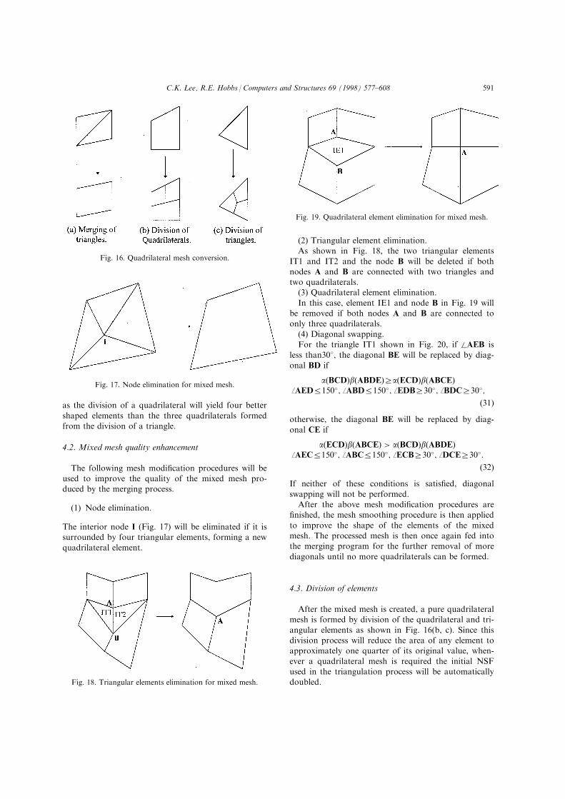
(2) Triangular element elimination.As shown in Fig. 18, the two triangular elements

IT1 and IT2 and the node B will be deleted if bothnodes A and B are connected with two triangles andtwo quadrilaterals.(3) Quadrilateral element elimination.

In this case, element IE1 and node B in Fig. 19 willbe removed if both nodes A and B are connected toonly three quadrilaterals.

(4) Diagonal swapping.For the triangle IT1 shown in Fig. 20, if {AEB is

less than308, the diagonal BE will be replaced by diag-

onal BD if

a�BCD�b�ABDE�ra�ECD�b�ABCE��AEDR150�; �ABDR150�; �EDBr30�; �BDCr30�;

�31�otherwise, the diagonal BE will be replaced by diag-onal CE if

a�ECD�b�ABCE� > a�BCD�b�ABDE��AECR150�; �ABCR150�; �ECBr30�; �DCEr30�:

�32�If neither of these conditions is satis®ed, diagonal

swapping will not be performed.After the above mesh modi®cation procedures are

®nished, the mesh smoothing procedure is then applied

to improve the shape of the elements of the mixedmesh. The processed mesh is then once again fed intothe merging program for the further removal of more

diagonals until no more quadrilaterals can be formed.

4.3. Division of elements

After the mixed mesh is created, a pure quadrilateralmesh is formed by division of the quadrilateral and tri-

angular elements as shown in Fig. 16(b, c). Since thisdivision process will reduce the area of any element toapproximately one quarter of its original value, when-

ever a quadrilateral mesh is required the initial NSFused in the triangulation process will be automaticallydoubled.

Fig. 16. Quadrilateral mesh conversion.

Fig. 17. Node elimination for mixed mesh.

Fig. 18. Triangular elements elimination for mixed mesh.

Fig. 19. Quadrilateral element elimination for mixed mesh.


4.4. Quadrilateral mesh quality enhancement procedures

After the pure quadrilateral mesh is formed, a series

of mesh modi®cation and smoothing procedures simi-lar to those used in refs [8] and [24] is then applied toimprove the quality of the quadrilateral mesh.

It should be pointed out that during all the abovemodi®cation and smoothing processes for triangular,mixed and quadrilateral surface meshes, whenever a

node or an element is moved, inserted or deleted,checks are performed to ensure that all altered el-ements will be valid elements in both the parametric

and 3D spaces.

5. Speed and Memory Considerations

When compared with 2D mesh generation, the sur-face mesh generator will incur a greater computational

cost for the following reasons:

1. Although most of the connectivity and intersection

checks can be done in the parametric space, manygeometrical parameters of the elements generated

must be computed in the 3D space for element

shape and grading control during both mesh gener-

ation and mesh quality enhancement.

2. A few time consuming steps, such as the determi-

nation of pseudo-midpoint and o�set directions, are

used during the surface element formation.

However, careful examination of all the mesh gener-

ation and enhancement processes shows that their op-

eration complexities are exactly the same as their 2D

counterparts and are as shown in Table 1. This feature

is due to the extensive use of the one-to-one mapping

relationship between the parametric space and the 3D

space so that the whole mesh generation process is

topologically equivalent to a 2D mesh generation pro-

blem.

These predictions are con®rmed by plotting the

actual CPU times used by di�erent generation pro-

cedures for some mesh generation examples: the results

are shown in Figs. 21±24. From these ®gures it can be

seen that the triangular mesh generation procedure is

the most time consuming procedure since nearly all the

most expensive operations are involved in the gener-

ation phase. Finally, it is noted that the speed of the

current generation process appears to be rather slow,

about 200 min for the generation of 15 000 elements

(the background mesh for that problem has about 14

000 elements), because all the examples shown here

were produced on a relatively small and slow 486DX2/

66 PC.

It is also found that the amount of memory required

is always proportional to the number of elements to be

generated. Under the current programming environ-

ment the memory required to generate a surface mesh

with 10 subsurfaces and a total of 30 000 elements (for

Fig. 20. Diagonal swapping for mixed mesh.

Table 1

Operation complexities for di�erent surface mesh generation

steps (NE= number of elements in the mesh)

Process

Order of operation

Complexity

Triangular mesh generation O(NE1.5)

Triangular mesh quality enhancement O(NE)

Quadrilateral mesh generation O(NE1.5)

Quadrilateral mesh quality enhancement O(NE)

Overall O(NE1.5)


both background mesh and new mesh) is about 15Mb.

6. Surface Mesh Generation Examples

In this section some examples will be presented todemonstrate the performance of the mesh generatordeveloped. The element size information of the ®niteelement meshes is directed by some ®ctitious NSFs

de®ned over the 3D domains. In all the examples, the

mesh generation procedure is started by computing thespeci®ed NSF over the nodal points of the initialmeshes, which is then fed into the generator for mesh

formation such that the situation during an adaptiveanalysis is directly imitated.

6.1. Mesh quality and grading assessment

In order to assess the quality of the elements gener-

ated, the a values (for triangles) and b values (for

Fig. 21. CPU time of triangular mesh generation against NE1.5.

Fig. 22. CPU time of triangular mesh quality enhancement against NE.


quadrilaterals) of the elements in the meshes are com-

puted, and the overall quality is measured by the geo-

metrical means a and b [8] of all the elements.

Furthermore, for a quadrilateral mesh, the distortion

of individual elements can also be assessed by consid-

ering the internal angles of the element in the 3D

space. For a quadrilateral element ABCD, the internal

angle at node B, denoted as WCBA, is de®ned as

WCBA � �CBA fj�CBAÿ 90�jrj�CBD� �DBAÿ 90�j�CBD� �DBA otherwise:

��33�

For a given element in a quadrilateral mesh, the shape

quality of that element is deemed satisfactory if all its

Fig. 23. CPU time for quadrilateral mesh generation against NE*log2(NE).

Fig. 24. CPU time of quadrilateral mesh quality enhancement against NE.


internal angles, W, fall within the interval [308, 1508].The mesh grading of the ®nal mesh obtained is

assessed by the di�erence between the desired element

size and the element size actually generated, using the

mesh grading coe�cient w de®ned in ref. [8].

6.2. Numerical examples

A total of ®ve surface domains has been discretized

by the proposed mesh generator. For each domain, a

pure triangular mesh and a pure quadrilateral mesh

Fig. 25. (a) Geometry for Surface 1; (b) initial mesh for Surface 1; (c) ®nal triangular mesh for Surface 1; (d) ®nal quadrilateral

mesh for Surface 1.


have both been generated. Subsurfaces of these

domains range from the trivial planar surface to some

heavily folded open and closed surfaces. Regardless of

such a great variation in the ``roughness'' of these sur-

faces, ®ve iterations were used in all the examples to

obtain the ®nal triangular and quadrilateral meshes.

The geometry of these surfaces, represented as plots of

their parametric nets with hidden line removal, is

shown in Fig. 25(a)±29(a). The initial coarse ®nite el-

ement meshes used to start the iterations are shown in

Fig. 25(b)±29(b). These initial meshes are so coarse

that none of them can be considered as an adequate

representation of the surfaces. The exact analytical

forms of these surfaces and the ®ctitious NSF used

will not be given here since they are lengthy but not

very informative. A more concise picture of the mesh

generation results can instead be obtained by studying

the quality and grading characteristics of the ®nal

meshes generated which are shown in Tables 2 and 3.

The ®nal triangular and quadrilateral meshes obtained

are shown in Fig. 25(c)±29(c) and Fig. 25(d)±29(d) re-

spectively.

From Figs. 25±29 and Tables 2 and 3 it can be con-

cluded that the overall mesh quality of all the meshes

generated is good. The a values of all triangular

meshes are greater than 0.9 while the b values of all

quadrilateral meshes are better than 0.65.

Occasionally, there are a few quadrilateral elements

with internal angles outside the range [308, 1508], butalways fewer than 0.2% of the total number of el-

ements in the mesh, and these with internal angles just

marginally outside the required range. It should be

mentioned that, in order to test thoroughly the ability

and robustness of the mesh generator, some of the ®c-

titious NSF used are deliberately designed to yield

unrealistically graded meshes which are not expected

to appear even in adaptive ®nite element analysis.

As for the grading of the meshes generated, it can

be seen that the w coe�cients for all triangular meshes

are good with values greater than 0.8. The w coe�-

cients of all quadrilateral meshes are slightly lower

than the corresponding values of their triangular

counterparts with the lowest one (Surface 1) just less

than 0.7. This e�ect can be seen by comparing corre-

sponding plots in Figs. 25±29 and also the element size

ratio in the last column of Tables 2 and 3. This

phenomenon can be explained by the following argu-

ment. A non-uniform mesh generated will never be

able to attain a perfect w coe�cient of 1 because the

mesh generated is always an approximation of the sur-

face and the speci®ed node spacing function. Hence,

by using the simple conversion scheme for the gener-

Table 2

Characteristics of ®nal triangular meshes generated

Surface number NSR NN NE a w Amax/Amin

1 [Fig. 25(c)] 2 5138 10240 0.922 0.830 15271.4

2 [Fig. 26(c)] 1 7599 14877 0.933 0.888 7468.6

3 [Fig. 27(c)] 1 7153 14994 0.964 0.904 79.1

4 [Fig. 28(c)] 2 4393 8680 0.953 0.894 2613.9

5 [Fig. 29(c)] 8 13171 26094 0.935 0.889 4632.4

NSR= number of subsurfaces of the problem domain; NN= number of nodes in the mesh; NE = number

of elements in the mesh; a=mean a quality of triangular mesh; �=mean b quality of quadrilateral mesh;

w =mesh grading coe�cient; Amax/Amin=ratio of maximum element size to minimum element size;

N1 = number of quadrilateral elements outside the range [308, 1508]; Wmin=minimum internal angle of all the

elements in the mesh; Wmax=maximum internal angle of all the elements in the mesh.

Table 3

Characteristics of ®nal quadrilateral meshes generated

Surface number NSR NN NE b N1 Wmin Wmax w Amax/Amin

1 [Fig. 25(d)] 2 5372 5354 0.698 7 24 155 0.694 4996.5

2 [Fig. 26(d)] 1 7779 7718 0.603 8 23 156 0.771 4914.5

3 [Fig. 27(d)] 1 7325 7174 0.762 0 31 145 0.858 150.6

4 [Fig. 28(d)] 2 5049 4996 0.720 6 24 154 0.849 2333.1

5 [Fig. 29(d)] 8 15463 15342 0.706 5 24 156 0.767 1139.4

NSR= number of subsurfaces of the problem domain; NN= number of nodes in the mesh; NE = number of elements in the

mesh; �=mean a quality of triangular mesh; �=mean b quality of quadrilateral mesh; w =mesh grading coe�cient; Amax/

Amin=ratio of maximum element size to minimum element size; N1 = number of quadrilateral elements outside the range [308,1508]; Wmin=minimum internal angle of all the elements in the mesh; Wmax=maximum internal angle of all the elements in the

mesh.


ation of quadrilateral mesh, the resolution of the ®rst

triangular mesh generated with double node spacing

will be lower than the corresponding normal size tri-

angular mesh. However, from the results listed in

Tables 2 and 3, one can see that the numbers of nodes

obtained for corresponding triangular and quadrilat-

eral meshes are approximately the same, and the num-

bers of quadrilaterals are roughly one half of the

Fig. 26(a) and (b).


number of triangles. The plots (Figs. 25±29) also con-

®rmed that the mesh patterns of the triangular meshes

are preserved in all the quadrilateral meshes.

Turning to the convergence characteristics of the

iterative process, it is found that the w coe�cient and

the number of nodes and elements in the generated

mesh converge to their ®nal values after two to three

iterations.

One ®nal point worth mentioning is that for some of

the examples given, the input NSF used is actually too

Fig. 26. (a) Geometry of Surface 2; (b) initial mesh for Surface 2; (c) ®nal triangular mesh for Surface 2; (d) ®nal quadrilateral

mesh for Surface 2.


Fig. 27(a) and (b).



mesh for Surface 3.


Fig. 28(a).


Fig. 28(b).


Fig. 28(c).



mesh for Surface 4.


Fig. 29(a and b).



mesh for Srface 5.


coarse in some regions on the surface, resulting insome barely acceptable representations over part of thesurfaces (e.g. Surface 2). This demonstrated the im-

portance of a suitable NSF for the ®nal mesh qualityand grading for a 3D surface mesh.

7. Conclusions and Future Investigations

In this paper, a new approach for constructing anadaptive ®nite element mesh using the advancing front

technique (AFT) for surfaces represented by rationalB-spline curves (RBSS) is presented. In the proposedmesh generation scheme, a major part of the gener-ation processes is done in the parametric space and the

operational complexity of the mesh generation schemeis exactly the same as its 2D counterpart.The major di�erence between the current scheme

and previous work is that the shape and size of an el-ement in the 3D space is carefully monitored in eachelement creation step. By exploiting the robustness of

an AFT mesh generation scheme, very distorted andtwisted elements are ®rst generated in the parametricspace and then well-shaped 3D surface elements areobtained by mapping the elements back to the 3D sur-

face. Although this procedure will inevitably lead to amore complicated element formation scheme andrequire additional computational e�orts when com-

pared with the direct mapping technique, it is appli-cable to a wide range of folded surfaces and is able togenerate meshes with node spacing compatible with

the speci®ed input node spacing function (NSF) evenfor some unrealistically strongly graded node spacingdistributions.

A simple, yet highly e�ective, mesh conversionscheme is used for converting the triangular mesh into

a pure quadrilateral mesh. Although such a conversion

procedure may slightly lower the mesh grading quality

when compared with direct generation, all the quadri-lateral meshes shown in the mesh generation examples

have acceptable grading.

The robustness of the mesh generation and quadri-

lateral conversion procedures has been tested by apply-

ing them to generate some strongly graded meshes onsome very convoluted surfaces, and in applications to

adaptive shell analysis [25]. Satisfactory results have

been obtained in all cases.

Finite element mesh generation over general 3D sur-

faces is a complicated and di�cult task and many po-tential areas for further development are listed below.

(1) Secondary reverse mapping of parametric space.

Even though in the current implementation the distor-

tion e�ects of the parametric mapping have been takeninto account and o�set layers are generated to avoid

the singular e�ect of degenerated lines, a further

increase in the robustness and the e�ectiveness of the

mesh generator may be obtained by using the second-ary reverse mapping technique [12].

(2) Generalization of the mapping procedure.

All the generation algorithms described in this studycan be applied to a more general mapping procedure

such that the target surface is de®ned by a general sup-

port surface [19] on which the region to be meshed isenclosed by a number of unambiguously de®ned and

connected boundary curves (Fig. 30).

(3) Quadrilateral mesh conversion algorithm.

Results given in the last section show the mesh con-

version scheme used may slightly reduce the mesh

Fig. 30. Generalization of mapping procedure using support surfaces.


grading of the ®nal quadrilateral mesh. Therefore, adirect conversion scheme, such as the systemic merging

approach [26], may perform better than the currentprocedure in terms of preserving the mesh grading.From the previous experience in 2D problems, the con-

trol of element shape along the domain boundary isvital to the overall quality of the mesh generated asthe boundary nodes will constrain and handicap many

ad hoc modi®cation procedures during the mesh qual-ity enhancement.

Acknowledgements

The ®nancial support of the Croucher Foundation

to the ®rst author is gratefully acknowledged.

References

[1] Peraire J, Peiro J, Morgan K, Zienkiewicz OC. Finite el-

ement mesh generation and adaptive procedure for CFD.

In: Proceedings of the GAMNI/SMAI Conference on

Automatic and Adaptive Mesh Generation. Grenoble,

France, October 1±2, 1987.

[2] Lo SH. A new mesh generation scheme for arbitrary pla-

nar domains. Int J Numer Meth Engng 1985;21:1403±26.

[3] George PL, Seveno E. The advancing-front mesh gener-

ation method revisited. Int J Numer Meth Engng

1994;37:3605±19.

[4] Shephard MS, Georges MK. Automatic three-dimen-

sional mesh generation by the ®nite octree technique. Int

J Numer Meth Engng 1991;32:709±49.

[5] Baehmann PL, Wittchen SL, Shephard MS, Grice KR,

Yerry MA. Robust, geometrically based, automatic two-

dimensional mesh generation. Int J Numer Meth Engng

1987;24:1043±78.

[6] Baehmann PL, Shephard MS, Flaherty JE. A posteriori

error estimation for triangular and tetrahedral quadratic

elements using interior residuals. Int J Numer Meth

Engng 1992;34:979±96.

[7] Zhu JZ, Hinton E, Zienkiewicz OC. Adaptive ®nite el-

ement analysis with quadrilaterals. Comput Struct

1991;40:1097±104.

[8] Lee CK. Automatic adaptive ®nite element mesh gener-

ation over 2D arbitrary domainÐa review. Progress

report, Department of Civil Engineering, Imperial

College of Science, Technology and Medicine, University

of London, 1994.

[9] Ghassemi F. Automatic mesh generation scheme for a

two or three-dimensional triangular curved surface.

Comput Struct 1982;15:613±36.

[10] Wu SH, Abel JF. Representation and discretization of

arbitrary surfaces for ®nite element shell analysis. Int J

Numer Meth Engng 1979;14:813±36.

[11] Gordon WJ, Hall CA. Construction of curvilinear co-

ordinate systems and applications to mesh generation.

Int J Numer Meth Engng 1973;7:461±77.

[12] Hinton E, Rao NVR, Ozakca M. Mesh generation with

adaptive ®nite element analysis. Adv Engng Software

1991;13:238±62.

[13] Potyondy DO, Wawrzynek PA, Ingra�ea AR. An algor-

ithm to generate quadrilateral or triangular element sur-

face meshes in arbitrary domains with applications to

crack propagation. Int J Numer Meth Engng

1995;38:2677±701.

[14] Okstad KM, Mathisen KM. Towards automatic adaptive

geometrically non-linear shell analysis. Part I: implemen-

tation of an h-adaptive mesh re®nement procedure. Int J

Numer Meth Engng 1994;37:2657±78.

[15] Lau TS, Lo SH. Finite element mesh generation over

analytical curved surfaces. Comput Struct 1996;59:301±9.

[16] Cass RJ, Benzley SE, Meyers RJ, Blacker TD.

Generalized 3-D paving: an automated quadrilateral sur-

face mesh generation algorithm. Int J Numer Meth

Engng 1996;39:1475±89.

[17] Piegl L, Tiller W. Curve and surface constructions using

rational B-splines. Comput Aided Des 1987;19:485±98.

[18] Lo SH. Automatic mesh generation and adaptation by

using contours. Int J Numer Meth Engng 1991;31:689±

707.

[19] Peraire J, Peiro J, Formaggia L, Morgan K, Zienkiewicz

OC. Finite element Euler computations in three dimen-

sions. Int J Numer Meth Engng 1988;26:2135±59.

[20] Bonet J, Peraire J. An alternating digital tree (ADT) al-

gorithm for 3D geometric searching and intersection pro-

blems. Int J Numer Meth Engng 1991;31:1±17.

[21] Lo SH. Generating quadrilateral elements on plane and

over curved surfaces. Comput Struct 1989;31:421±6.

[22] Herrmann LR. Laplacian-isoparametric grid generation

scheme. J Engng Mech Div ASCE 1976;12:749±59.

[23] Rank E, Schweingruber M, Sommer M. Adaptive mesh

generation and transformation of triangular to quadrilat-

eral meshes. Commun Numer Meth Engng 1993;9:121±9.

[24] Zhu JZ, Zienkiewicz OC, Hinton E, Wu J. A new

approach to the development of automatic quadrilateral

mesh generation. Int J Numer Meth Engng 1991;32:849±

66.

[25] Lee CK, Hobbs RE. Automatic adaptive re®nement for

shell analysis using nine node assumed strain element.

Int J Numer Meth Engng 1997;40:3601±38.

[26] Lee CK, Lo SH. A new scheme for the generation of a

graded quadrilateral mesh. Comput Struct 1994;52:847±

57.


automatic adaptive finite element mesh generation over rational b-spline surfaces

Documents