automatic analysis and correction of hvac system simulated performance: a cooling coil ... ·...

Loughborough UniversityInstitutional Repository

Automatic analysis andcorrection of HVAC systemsimulated performance: acooling coil case study

This item was submitted to Loughborough University's Institutional Repositoryby the/an author.

Citation: WRIGHT, J.A. and BOUGHAZI, L., 1990. Automatic analysis andcorrection of HVAC system simulated performance: a cooling coil case study.ASHRAE Transactions, 96(2), pp.743-749

Additional Information:

• This is a journal article [ c© American Society of Heating, Refrigeratingand Air-Conditioning Engineers, Inc. 2005] (www.ashrae.org). Reprintedby permission from ASHRAE Transactions. This material may not becopied nor distributed in either paper or digital form without ASHRAE'spermission.

Metadata Record: https://dspace.lboro.ac.uk/2134/5032

Version: Published

Publisher: c©American Society of Heating, Refrigerating and Air-ConditioningEngineers, Inc.

Please cite the published version.

https://dspace.lboro.ac.uk/2134/5032

This item was submitted to Loughborough’s Institutional Repository (https://dspace.lboro.ac.uk/) by the author and is made available under the

following Creative Commons Licence conditions.

For the full text of this licence, please go to: http://creativecommons.org/licenses/by-nc-nd/2.5/

SL-90-10-4

AUTO AT|C ANALYSIS AND CORRECT|ON OFHVAC SYSTEIVi $| ULATED PERFORMANCE:A COOL|NG CO|L CASE STUDY

J.A. Wright, Ph.D. L. Boughazi

ABSTRACTCurrent HVAC system simulation software is sufficiently

accurate and flexible to be of use in system design. Its integra-tion into the design process is hindered, however, by the needfor extensive analysis of the simulation output and by difficultiesin taking action to correct system performance if this is initiallypoor. The first section of this paper gives an overview of the useof intelligent knowledge-based software in the automatic anal-ysis and correction of the simulated performance of HVACsystems. The second section describes an implementation forthe steady-state simulation of a proportionally controlled cool-ing coil.

iNTRODUCTIONRecently, there has been a rapid expansion in the develop-

ment of software for the simulation of the thermal performanceof heating, ventilating, and air-conditioning (HVAC) systems(Murray 1985; Day et al. 1986; Clark and May 1985; Sowell etal. 1986). Much of the research to date has been concernedwith the development of modeling and solution procedures,and, although a user-simulation interface has been developed(Clarke and Rutherford 1988), attention has only recently beenpaid to the way in which the software is used to perform theanalysis and improve designs. This has led to software that isvery sophisticated in terms of modeling flexibility but gives lit-tle assistance in the analysis of results or guidance on possi-ble improvements in system design.

HVAC System Simulation and DesignHVAC system performance simulation software is used at an

early stage of design to predict the performance and operationof the system. This is particularly important in relation to noveland innovative designs, where experience with the installedperformance of the system is unknown or limited. The first stepin a simulation exercise is to define the system configuration,set design conditions (such as fluid mass flow rates), and selectappropriate sizes of components. The selection of the designconditions and component sizes is normally made through aconventional working design procedure in isolation of the simu-lation. Following the simulation of system performance, twooperations are required to improve the system design:1. The operation and performance of the individual compo-

nents and of the system as a whole are analyzed and anassessment is made as to the suitability of the system.

2. If the system performance is unsatisfactory, then it is cor-rected by changing the size of the system components and/or design conditions. In some instances, it may be neces-sary to select a different system type.

Once the corrections have been made, the system perfor-mance can be re-simulated and re-analyzed, with further cor-rections and analysis made if necessary. This iterative processis time-consuming, requires in-depth knowledge on behalf ofthe user, and often involves operations that are external to thesimulation, such as cross-references to manufacturers’ cata-logs in order to make improved equipment selections. It is evi-dent that the effectiveness of the simulation software as adesign tool can be improved by automating the analysis andcorrection of the system’s performance.

AUTOMATIC ANALYSIS AND CORRECTIONOF SYSTEM PERFORMANCE

There is no generalized approach to analyzing and correct-ing the simulated performance of HVAC systems. Each user ofthe software will adopt a different and in some cases arbitraryor trial-and-error approach that is directed more by intuitionthan by fact. The factors considered by the users will varyaccording to the project at hand; for instance, system efficiencymay be of little importance so long as close control is main-tained.

Analysis of Design Conditions andHVAC System Performance

HVAC system simulated performance cannot be analyzed incomplete isolation from the choice of design conditions and theform of simulation. Three levels of analysis can therefore beidentified:1. Analysis of the cause of failure of the simulation, should this

OCCUE2. Analysis of the system’s performance.3. Analysis of the choice of design conditions and component

selections.Failure of the Simulation Failure of the simulation is often

due to the poor sizing of components or bad choice of designconditions, as this can produce an insoluble set of system equa-tions. The cause of failure may be identified from the simula-tion output, as it is often evident that the solution had placedthe operating point of a component beyond its performancelimit. The extent to which any output from a failed simulation isof use depends upon the particular simulation solution proce-dure. In some instances, it is possible to assess the choice ofcomponent size and design constraints (such as the fluid veloc-ities at peak flow).

Analysis of System Performance HVAC system perfor-mance is defined here to mean the operation and efficiency ofthe system. Four factors are often considered in relation to sys-tem performance:

J.A. Wright is a Lecturer and L. Boughazi is a Research Student in the Department of Architecture and Building Engineering, TheUniversity, Liverpool, England.

743

© 1990. American Society of Heating, Refrigerating and Air-Conditioning Engineers, Inc. (www.ashrae.org). Published in ASHRAE Transactions Vol. 96, Part 2. For personal use only. Additional reproduction, distribution, or transmission in either print or digital form is not permitted without ASHRAE’s prior written permission.

1. The maintenance of system control for both individual com-ponents and, in sequencing of control, from one componentto another (local loop and supervisory control).

2. The compliance with design constraints, such as limitingfluid velocities.

3. The provision of acceptable residual operating capacity.4. Efficient and economical system operation.

Many of these factors can be assessed for each componentand judged against a readily available rule of thumb. Thosefactors that are assessed at system level are, however, lessgenerally defined and can be specific to a particular system’sconfiguration. The sequencing of control, for instance, is spe-cific to the type of air-conditioning system.

Analysis of the Design Conditions and Component SizeThe separate analysis of the design conditions and componentsize is important on two accounts: First, to interpret the causeof any poor performance, which is offen less than obvious andalways involves some inference. Second, the choice of designconditions and component selections must be assessedagainst current working practice, since it is possible that a badcombination of design conditions and component sizes couldproduce a seemingly satisfactory performance. Rules of thumbare available for evaluating the design conditions, but few or norules of thumb are available for assessing the physical size ofthe components. Rules for analyzing component size could beformulated by relating the component’s operating point to thelimits of its performance map or through developing a sizedescriptor from first principles.

HVAC System Performance CorrectionCorrection of system design follows the performance anal-

ysis. Providing that a change in system type is not suggested,the system performance can be corrected by changing thevalues of the design conditions and by resizing the compo-nents~ Rules of thumb are available for evaluating the designconditions, but few, if any, simple rules exist for specifying thephysical size of the components.

The correction to system performance is further complicatedby the thermofluid coupling between the components, asthough this change to one component or design condition willaffect the performance of other components in the system. Thiseffect also applies to individual components when the compo-nent size is described by more than one parameter.

The correction process itself can be approached in severalways: the correction of cornponent size and the design param-eters could be based on simple rules formulated in associationwith the rule for assessing performance. A second possibleapproach is to implement the component selection proceduresemployed by the equipment manufacturers to produce work-ing designs. Finally, the correction could be based on anoptimal design procedure, which, for example, gives solutionswith the lowest capital cost.

~mp~ementation for AutomaticAnalysis and Correction

Both analysis and correction of system perforrnance requirelarge amounts of expertise and knowledge. Much of this knowl-edge can be represented by simple rules and facts and throughinference. Whereas most simulation software is written in a pro-cedural programming language, the facts, rules, and inferencerequired for the analysis and correction of system performanceare best implemented using an intelligent know!edge-basedlanguage. If the optimal correction of system performance isrequired, additional procedural calculating routines are neces-sary to perform the optimization. These routines could be di-rected or accessed by the intelligent knowledge-basedsoftware. The interfacing of two different languages can bedifficult, although in most cases either the languages will per-mit this directly or the linking can be achieved through thecomputer’s operating systern. Each simulation program has its

own component model format, systern definition procedure,and solution procedure. Due to these differences, any auto-rnatic performance analysis and correction procedure will bespecific to the simulation program. This is not to say that a basictemplate containing the knowledge common to all simulationprograms could not be developed.

COOLING COBL CASE STUDYThe attributes of the automatic analysis and correction

process have been informed through a cooling coil case study(Boughazi 1989). Figure 1 illustrates the system simulated. Thecoil is proportionally controlled by the action of a three-portdiverting valve; the control variable is the dry-bulb temperatureleaving the coil. The size of the coil is defined by the numberof rows, nurnber of water circuits, and the coil’s width andheight; the fin spacing is fixed in the sirnulation at 315 fins/m.The air condition entering the coil and water inlet condition tothe valve are defined by the user, as are the setpoint and propor-tional band of the controller. The hydraulic performance of thesystem is excluded from the simulation; the control valve is,therefore, assumed to have a linear installed characteristic.

Cooling coil

[ma]

[tai]

[gai]

tao

gao

~Thermostat

two

Diverting [pb]valve

Proportionalcontroller

[mwmax]

[twi]

Figure 1 Proportionally controlled cooling coil. Variables in[] are fixed during the simulation.

The objective of the study is to investigate the feasibility ofanalyzing and correcting the peak-load performance of the coilusing only simple rules of thumb rather than extensive designcalculations. The coil’s performance is defined in terms of:1. Maintenance of control (steady-state control error).2. Compliance with air face and water velocity limits.3. Provision of acceptable residual operating capacity.

The analysis of the design conditions and component sizeis restricted to:1. The water flow rate at peak load.2. The coil size, which is not defined in relation to any specific

dirnensions but is implied to mean the total heat transfer sur-face area.

The parameters that can be changed to correct an indicatedpoor performance are:1. The water mass flow rate at peak load.

2. The coil width, height, number of rows, and number of watercircuits.

744


The Simulation ModelThe simulation model implemented is steady state and is

based on the British Standard test and performance calcula-tion method (B.S. 5141, 1975). The standard adopts the "threeline" calculation method, which simulates three modes of heattransfer on the air side of the coil: a dry surface, a partially wetsurface, and a wet surface. The system performance is simu-lated by using a successive approximation algorithm to iterateon both the coil water mass flow rate and the coil air outlet tem-perature. The simulation is generally robust, although it can failwhen the operation of the coil lies between modes of heat trans-fer (e.g., between a wet or partially wet surface) or when theoperation is outside the limit of the modeled range of heat trans-fer coefficient on the air side of the coil (a face velocity of morethan 5.0 m/s).

Knowledge Acquisition, SimplifyingAssumptions, and Limitations

Rules for the analysis and correction of cooling coil perfor-mance have been obtained from published rules of thumb (Hay-ward 1988) and through a knowledge of cooling coil design inpractice and through experience in operating the simulation°

In order to reduce the scope of the analysis and correctionto a manageable level, several simplifying assumptions havebeen made. The effect of the controller’s proportional band isnot analyzed, nor is it used to correct system performance sinceits effect on the system’s stability is not reproduced by thesteady-state simulation. Similarly, the suitability of the coil flowwater temperature is not considered in the analysis or duringperformance correction, since its effect on chiller performancecannot be assessed as the chiller is not part of the systemsimulated. Finally, the analysis and correction are for the peakload on the coil, as this is when the coil performance is testedto its limit.

The size of a coil is not only described by the physical width,height, and number of rows but also by the number of water cir-cuits. The correctness of coil size in relation to any one of theseparameters is influenced by one or more often-competingdesign constraints. The coil height, for instance, can be dictatedby the amount of heat transfer surface area required to main-tain control as well as the limiting face velocity. In light of thesedifficulties, the analysis and correction of coil size has been sim-plified. The analysis of size is purely through inference, with coil"size" implied to mean the total heat transfer surface area. Thecorrection procedure for the physical size of the coil is similarto cooling coil design methods in practice; namely, width andheight are used to correct the coil face velocity, the number ofwater circuits to correct the water velocity, and the number ofrows to correct the heat transfer surface area.

The cause of the simulation failure is not included in the auto-matic analysis. The parameters that can be assessed on failureof the simulation are the maximum air face and water veloci-ties and the choice of maximum water flow rate.

Rules for Performance AnalysisThe parameters inchJded in this analysis are: maintenance

of control in the steady state, the compliance with design con-straints, and the coil’s residual operating capacity.

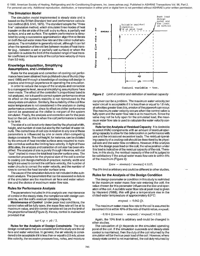
Maintenance of Control Under peak load conditions, thecontrol valve will be fully open, the mass flow rate will be at itsmaximum value, and the control variable will be on the limit ofthe proportional band (Figure 2). Hence, control is maintainedprovided that

tao <~ sp + pb / 2.

Rules for the Analysis of Design Constraints The onlydesign constraints that are considered in this study are the airface and water velocities. In general, the air velocity is consi-dered to be acceptable if it is less than or equal to 2.5 m/s; abovethis velocity, the excessive pressure loss, noise, and moisture

I

14

0

o

~Suitable residualcapacity,5%_ at_pe_ak_ l_oa_d-

I!

!

~P

Peak loaddesignpoint andthe limitof control

Control variable - tad.

Figure 2 Limit of control and definition of residual capacity

carryover can be a problem. The maximum water velocity perwater circuit is acceptable if it is less than or equal to 1.8 m/s;at velocities greater than this, erosion of the pipework can occur.The maximum water velocity occurs when the control valve isfully open and the water flow rate is at its maximum. Since thevalve may not be fully open for the simulated load, the maxi-mum water flow rate is used to calculate the water velocity con-straint.

Rule for the Analysis of Residual Capacity It is desirableto select HVAC components with an amount of residual oper-ating capacity to allow for the deterioration in performance withuse and the occasional excessive loads. The residual operat-ing capacity of a cooling coil should be described by its physi-cal size and the water flow conditions. However, if the analysisis for the design peak load on the coil, the valve position underthis load is indicative of the residual capacity of the coil. There-fore, in this study, the residual capacity of the coil is judged tobe satisfactory if the actual water mass flow rate is within 5%of the maximum (Figure 2):

[(mw - mwmax) / mwmax] <~ 0.05.

The 5% limit is arbitrary and could be different in other studies.

Rules for the Analysis of the Design ConditionThe design parameter or condition in this study is restricted

to the maximum water mass flow rate entering the coil; thevalue chosen for this parameter influences the size and oper-ation of the coil. A suitable water flow rate at peak load is givenby Hayward (1988); this will give a temperature rise in thechilled-water temperature of approximately 6.0°C:

mwpeak = 0.042 Qto

The maximum water mass flow rate to the coil is assumed tobe correct if it is within 10% of the rule-of-thumb value, mwpeak:

-O.lO ~< [(mwmax - mwpeak) / mwpeak] <~ 0.10o

Again, the 10% limit is arbitrary and could be changed inother studies.

The calculation of Qt depends on the simulated operatingpoint of the coil. If the simulation succeeds and steady-statecontrol is maintained, then the duty of the coil returned by thesimulation will be the true peak load of the coil. However, wheresteady-state control is not maintained, the coil duty returned by

745


the simulation will be less than the true peak duty; here, thepeak duty can be estimated frorn:

Qt = ma Cp (sp - tai) / shr:

If the simulation should fail, then the sensible heat ratio isunavailable and an "in the order of" value must be defined. Thevalue of 0.6 has been selected as a typical sensible heat ratiofor this study.

Ru~es for Analyzing Coil SizeCoil "size" is implied here to mean the total heat transfer sur-

face area. Since few, if any, simple rules of thumb exist forassessing coil size, the approach adopted in this study is to useinference to judge the suitability of coil size. The performanceof a coil is dependent on both the water mass flow rate and coilsize. The choice of coil size can, therefore, be inferred from thecoil performance and choice of water flow rate, since these canbe separately analyzed. For instance, if the coil performanceis correct and yet the water mass flow rate is found to be low,then the coil must be oversized to cornpensate for the reducedwater mass flow rate~ This approach is limited on two accounts:First, the coil size cannot be analyzed in all cases, most nota-bly, if the coil performance is poor and the water mass flow rateis low, then it is not possible to infer that the coil is also under-sized. Second, the individual parameters of coil size, such aswidth and height, cannot be assessed in relation to the amountof heat transfer surface area. The rules for coil size analysis areas follows:

The coflsize is correct if control is maintained, the residualcapacity is correct, and the water mass flow rate is correct.

The coil is undersized if control is maintained, the residualcapacity is correct, and the water mass flow rate is high, or, ifcontrol is not maintained and the water mass flow rate is highor correct.

The coil is oversized if control is maintained and the watermass flow rate is low, or, if control is maintained, the residualcapacity is high, and the water mass flow rate is correct.

Rule for Correcting the Design ConditionThe maximum water mass flow rate to the coil can be reset

by assigning it the value derived from the rule of thumb usedin the analysis:

mwmax = mwpeako

Rules for the Correction of Coil SizeThe correction of coil size could be initiated either directly

frorn the analysis of size or in order to correct an indicated poorperformance. Since coil size is defined by several parametersand no simplified rules exist for correcting coil size, the sourceof correction for’ each parameter has been selected in relationto current working practice. The main elements are that coilwidth and height are corrected to give a satisfactory face veloc-ity; the number of water circuits is corrected to produce a satis-factory water velocity; and the number of coil rows is adjustedto correct an indicated under- or oversizing of the coil.

Correction to Coil Width and Height The coil width andheight are corrected to give a face velocity equal to the limitingvelocity. To simplify the calculation, a square face area isassumed:

Af = ma. spvol / vf .......................................

Width = Height = Af°5.

Correction to the Number of Water Circuits The numberof water circuits is corrected to give a water velocity equal to thelimiting velocity:

Ncirc = mwmax / p .Ai. vw.

Correction to the Number of Coil Rows The rules of thumbfor’ correcting coil size have been developed more through intu-ition than adherence to standard design methods. The partic-ular rule applied for correction depends on the inference usedto identify incorrect sizing. The strategy for correcting an under-sized coil is as follows:

If control is maintained but the water mass flow is high, thenthe coil rows can be increased in proportion to the proposedreduction in water flow rate, provided that the correction is notso great that the nonlinearity in the relationship between coiloutput, water mass flow rate, and the number of rows becomessignificant:

Nrow = Nrow [1 + (mwmax - mwpeak) / mwmax].

Where control is not maintained and the water mass flow rateis correct or high, then a better indication of tile correction tothe number of rows required is by a comparison of the air out-let ternperature and the setpoint temperature. The water inlettemperature is also included in this rule, since the differencebetween the air and water temperature is an indication of thedriving force for heat transfer:

Nrow = Nrow (tao - twi) / (sp - twi).

Similarly, in correcting an oversized coil, the strategydepends on the inference used to identify oversizing. Thestrategy for correcting oversizing is as follows:

If control is maintained but the maximum water mass flowrate is low, then the number of coil rows can be corrected inproportion to the proposed increase in water rnass flow rate:

Nrow = Nrow (mwpeak - mwmax) / mwmax.

Where control is maintained, the water mass flow rate is cor-rect, but the residual capacity is high, then the coil rows can bedecreased in proportion to the required reduction in residualcapacity. Since the residual capacity is defined in terms of theactual and maximum possible water flow rates through the coiland as the flow rate is to be within 5% of the maximum, thenthe correction to the number of rows is given by:

Nrow = Nrow [row / (0.95. mwmax)].

~mplernentationThe rules for analysis and correction have been implemented

using the declarative programming language PROLOG Thisis interfaced to the cooling coil simulation written in FORTRANby a routine written in ASSEMBLER. A mainframe cornputerhas been used to run the software. "[’he software is enteredthrough the PROLOG routines, and a menu structure allowsprogram control. The user may specify the peal( load on the coiland the coil width, height, number of rows, and number of watercircuits for the initial analysis and correction.

Following an initial analysis of perforrnance, the user maycorrect a single parameter (such as coil size), after which thesimulation is re-run and the performance re-analyzed. A"correct-all" option corrects each parameter in turn, re-runningthe simulation and re-analyzing performance after each correc-tion. The process iterates until the parameter is correct. Theorder of correction is:

1. Width and height based on the face velocity.2. Nurnber of water circuits based on the water velocity.30 Number of rows based on the coil size as analyzed.

The backward-chaining inference mechanism of PROLOGis suited to the task of performance analysis and correction,although a forward-chaining mechanism may simplify theimplementation for interpreting the cause of an indicated poorperformance.

746


TABLE 1Example Coil Load Data

Variable Datama 6.5 kg/stat 28.0°Cgai 0.0145 kg/kgtwi 8,0°Csp 12.0°Cpb 1~0°C

TABLE 2Example Coil Sizes and Design Conditions for Analysis

(Example 3 represents the "ideal" solution)

Example

Number of Coil Coil Number of MaximumCoil Rows Width Height Water Water Mass

(m) (m) Circuits Flow Rate(kg/s)

1 5 1.52 1.52 26 12.02 5 1.52 ’1.52 26 5.03 5 1.52 1.52 26 8.14 10 2.00 2.00 10 12.05 10 1o52 1.52 25 5o06 10 2.00 2.00 26 8. 17 2 1,00 1.00 10 12r08 2 1.00 "1 o00 26 5.09 2 1.52 1.52 26 8.1

Example Analysis and CorrectionThe effectiveness of the software in performing the analysis

and correction has been tested against several examples. Theload on the coil and the controller setpoint remain the same ineach example presented here (Table 1). Table 2 gives the exam-ple coil sizes and water mass flow rates. Table 3 presents theoutput from the simulation for each example; the output dataare incomplete for examples 4 and 7, since the simulation failedto find a solution, limiting the usable output data. Table 4 givesthe conclusions drawn from the analysis and the correct, orexpected, conclusions where this differs. Table 5 gives the coilsizes after the correction process.

The examples have been selected to test all possible com-binations of high, low, and correct maximum mass flow rate,with oversized, undersized, and correct coil size (Table 4). Con-ditions to test the conclusions drawn for coil performance arescattered arbitrarily within the set of examples. Example 3represents the "ideal" solution, since this coil’s performanceand size are "satisfactory."

Analysis of Coil Performance In general, the rules for anal-ysis proved to be satisfactory, with the only major limitationbeing the ability to evaluate coil size (heat transfer surface area)for all conditions. Where the simulation fails to find a solution(examples 4 and 7), it is not possible to assess the level

control, residual capacity, or coil size, since the data availablefor analysis are insufficient. Two minor errors were identifiedafter the implementation of the software, namely, that a checkfor low water and air face velocity is not included in the analy-sis; similarly, the analysis does not check for an insufficientresidual capacity. These simplifications account for the differ-ences between the expected and actual conclusions for theseparameters (Table 4).

The rules for assessing the choice of water mass flow ratehave been successful, except for example 8, where the coil wasso undersized that only sensible cooling occurred, giving areduced coil duty and assessment of mass flow rate. This errorcan be corrected by setting a typical coil sensible heat ratiowhen the simulation shows no dehumidification but dehumidifi-cation is expected.

The inference-based rules for analyzing coil size proved tobe limiting in three examples. In example 1, it is not possible toinfer if the high residual capacity of the coil is a result of boththe water mass flow rate and coil size; indeed, if the water massflow rate is high enough, then the coil could even be under-sized. Similarly, if the water mass flow rate is low and theresidual capacity is low or correct and control is lost (as in exam-ple 2), then it is impossible to infer if the lack of control is alsodue to an undersized coil. This would also apply to example 8had the water mass flow rate been judged as low instead of cor-rect. In this case, example 8 illustrates that rules that rely purelyon inference can draw incorrect conclusions when an error ina preceding judgment is made.

Correction to Coil Size and Water Mass Flow Rate Table5 gives the final corrected coil sizes and water mass flow ratesand the number of times the coil performance was re-analyzedto reach the final corrected conditions. The correction to watermass flow rate was successful in all examples except example7; here the water mass flow rate is 12% higher than the correctvalue, although it is within 10% of the calculated rule-of-thumbvalue against which it was assessed. The oversized coil widthand height in examples 4 and 6 were not corrected, since thecorrection is based on the coil f~ce velocity and no rules wereincluded to indicate a low face velocity with consequent over-sized width and height. The correction to the number of watercircuits was successful in all examples.

The correction to the number of coil rows was successfulexcept where the coupling between the coil width, height, andnumber of rows became critical. In examples 4 and 6, the widthand height were oversized, which led to a reduction in the num-ber of coil rows and a final judgment of an oversized coil. Simi-larly, in example 8, the width and height are slightly less thanthe ideal solution (example 3), which led to an increase in thenumber of rows. The conclusion here is that although the rulesfor correcting coil size are suitable for making crude correc-tions, the coupling between coil width, height, water circuits,and water mass flow rate must be considered in order toachieve a final correct solution.

TABLE 3Simulation Output Data

ExampleSimulationSolutionFound?

ContmlVariable(tao, °C)

Air Face Maximum Water Water MassVelocity Velocity Flow Rate(m/s) (m/s) (mw, kg/s)

Rule ofThumb Flow

(mwpeak, kg/s)

Sensible DutyHeat Ratio (kW)

(shr)1 YES 12.2 2,5 1.8 8.6 8.4 0,5 201.62 YES 14.4 2.5 1ol 5.0 8.5 0.5 165.63 YES 12.5 2.5 1.7 8~0 8°3 0.5 197,74 NO -- 1.4 6.6 -- 7.7 -- --5 YES 12.4 2.5 1.1 4.2 8.2 0.5 195.86 YES 11.9 1.4 1 r7 4.1 8.5 0.5 203.27 NO -- 5.7 6°6 -- 7.7 -- --8 YES 18.4 5.7 ’1.’1 5.0 4~6 1 ~0 63.59 YES 18.5 2.5 1,7 8.1 8.7 0.5 ’117.2

747


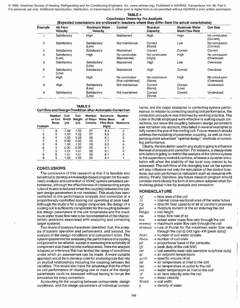
TABLE 4Conclusion Drawn by the Analysis

(Expected conclusions are enclosed in brackets where they differ from the actual conclusions)Example Air Face Maximum Water Control Residual Maximum Water Coil Size

Velocity Velocity Capacity Mass Flow Rate1 Satisfactory High Maintained High High No conclusion

(Correct)2 Satisfactory Satisfactory Not maintained Correct Low No conclusion

(Low) (None) (Correct)3 Satisfactory Satisfactory Maintained Correct Correct Correct4 Satisfactory High No conclusion No conclusion High No conclusion

(Low) (Maintained) (High) (Oversized)5 Satisfactory Satisfactory Maintained High Low Oversized

(Low)6 Satisfactory Satisfactory Maintained High Correct Oversized

(Low)7 High High No conclusion No conclusion High No conclusion

(Not maintained) (None) (Oversized)8 High Satisfactory Not maintained Correct Correct Undersized

(Low) (None) (Low)9 Satisfactory Satisfactory Not maintained Correct Correct Undersized

(Low) (None)

TABLE 5Coil Size and Design Condition after Automatic Correction

Example

Number Coil Coil Number Maximum Numberof Coil Width Height of Water Water Mass ofRows (m) (m) Cimuits Flow Iterations

(kg/s)1 5 1.52 1.52 27 8~4 22 5 1 °52 1 ~52 27 8.5 23 5 1.52 1.52 26 8.1 04 4 2.00 2.00 24 7.7 45 5 1 °52 1.52 26 8.2 46 4 2.00 2~00 26 8ol 27 5 1.51 1.51 28 9.1 58 6 1 ~51 1 ~51 26 8.1 49 5 1.52 1.52 26 8ol 1

CONCLUSIONSThe conclusion of this research is that it is feasible and

beneficial to develop a knowledge-based program for the auto-matic analysis and correction of HVAC system simulated per-formance, although the effectiveness of implementing simplerules of thumb is reduced when the coupling between the sys-tem design pararneters is not modeled. This study has beenrestricted to the performance analysis and correction of aproportionally controlled cooling coil operating at peak load.Although the study is for a single component, the design of acooling coil is sufficiently complicated for the coupling betweenthe design parameters of the coil dimensions and the maxi-mum water rnass flow rate to be representative of the charac-teristic problems associated with analyzing and correctinglarger systems.

Two levels of analysis have been identified: first, the analy-sis of system operation and performance, and second, theanalysis of the design conditions and component sizes. Therules implemented for assessing the performance of a coolingcoil proved to be reliable, except in assessing the suitability ofcomponent size (heat transfer surface area). Here the analysisis based on inference that has limited the range of conditionsunder which an assessment can be made. A more suitableapproach would be to develop rules for analyzing size that relyon explicit relationships including the coupling between thevariables. This would also have the advantage that the effecton coil performance of changing one or more of the designparameters could be assessed without having to re-run thesimulation for every correction.

Accounting for the coupling between components, designconditions, and the design parameters of individual compo-

nents, are the major obstacles in correcting system perfor-rnance. In relation to correcting cooling coil performance, thecorrection procedure was informed by working practice. Therules of thumb employed were effective in making crude cor-rections, but since the coupling between design pararneterswas not taken into account, they failed in several examples tofully correct the size of the cooling coil. Future research shouldaddress the rnodeling of pararneter coupling, as well as incor-porating more advanced "optimal design" methods of correct-ing performance.

Clearly, the simulation used in any study is going to influencethe level of analysis and correction. For instance, a steady-statesimulation is going to restrict the analysis of the control systemto the supervisory control functions, whereas a dynamic simu-lation will allow the stability of the local loop control to beassessed. The definition of the changing load on the systemwill also influence not only the simulation of the control func-tions, but also performance indicators such as seasonal effi-ciency. Finally, therefore, any future research program shouldconsider rnore closely the form of simulation adopted when for-mulating global rules for analysis and correction.

NOMENCLATURE

gaiHeightmamwmwmaxmwpeak

NcircNr o w

pbQts~rspspvoltaitaotwivfvwWidthp

= face area of the coil= internal cross-sectional area of the water tubes= specific heat capacity of air at constant pressure-- moisture content of the air entering the coil= coil height= mass flow rate of air= actual water mass flow rate through the coil= maximum water flow rate through the coil= rule of thumb for the maximurn water flow rate

through the coil (0.042 kg/s. kW [peak duty])= number of coil water circuits= number of coil rows= proportional band of the controller= peak duty of the coil (kW)= coil sensible heat ratio (sensible duty/total duty)= air setpoint temperature= specific volume of air= air temperature at inlet to the coil= air temperature at outlet to the coil= water temperature at inlet to the coil= air face velocity onto the coil= water velocity= coil width= density of water

748


REFERENCESBoughazi, L. 1989. "Intelligent knowledge based program

analysis and correction of HVAC system performance." M.S.thesis, The University of Liverpool, England.

B.S. 5141.1975. "Specification for air heating and cooling coils;Part 1. Methods of testing for rating of cooling coils." London:British Standards Institution.

Clark, D.R., and W.B. May. 1985. HVACSIM+ building systemsand equipment simulation program--User’s guide. Gaithers-burg, MD: National Institute of Standards and Technology.

Clarke, J.A., and J. Rutherford. 1988. "An intelligent front-endfor building energy simulation." User 1, A Working Confer-ence for Users of Simulation Hardware, Software and Intel-fiware, pp. 165-171. Ostend, Belgium.

Day, B., D. Richardson, and P. Kimber. 1986. "A modular sys-tem for sim ulation of the thermal performance of buildingsand their services systems." Department of MechanicalEngineering, University of Bristol, U.K.

Hayward, R.H. 1988. "Rule of thumb, examples for the design ofair systems." BSRIA Technical Note 5/88. Bracknell, England:Building Services Research and Information Association. ̄

Murray, M.A.P. 1984. "Component based performance simu-lation of HVAC systems." Ph.D. thesis, University of Technol-ogy, Loughborough, U.K.

Sowell, E.F., W.F. Buhl, A.E. Erdem, and F.C. Winkelmann.1986. "A prototype object-based system for HVAC simula-tion." Proceedings of the International Conference on SystemSimulation in Buildings, Liege, pp. 471-520.

DISCUSSION

Jeff Haberl, Department of Mechanical Engineering,Texas A&M University, College Station: Can you commenton your impression of the U.K. HVAC-KBS research and thecomparison to U.S. HVAC-KBS research?

749


automatic analysis and correction of hvac system simulated performance: a cooling coil ... ·...

Documents