IT Carlow - BSc.

Software development

Automatic Detection of

Brand Logos

Final Report

Student Name: Zhe Cui

Student Number: C00266169

Lecturer: Paul Barry

Date: 30.04.2021

Abstract

Automatic Detection of Brand Logos is a tool identifying brand logos in still and

moving images, and calculate how long the logo is visible. It can not only identify

10 different brands, 5 international brands and 5 Chinese brands, (Adidas, Kappa,

New Balance, Nike, Puma, 361, Anta, Erke, Lining, Xtep) but also locate the logo

that has not been seen before, the logo that has not been trained. Giving the

specific logo image, the system can mark the location of the logo in the pictures

and videos. This document contains the development process for Automatic

Detection of Brand Logos.

Table of Contents

1 Introduction .................................................................................................... 1

2 The project design ......................................................................................... 1

3 Logo detection data set construction ............................................................. 2

3.1 Analysis of existing open data sets ...................................................... 2

3.2 Dataset collection................................................................................. 4

3.2.1 Logo type selection .................................................................... 4

3.2.2 Web Crawling Tools to get data .................................................. 4

3.2.3 Manually label data .................................................................... 5

4 The parameters of performance evaluation in the object detection ................ 8

4.1 Intersection-over-Union (IoU) ............................................................... 8

4.2 TP TN FP FN ..................................................................................... 10

4.3 Precision and recall ............................................................................ 10

4.4 Example .............................................................................................. 11

4.5 Limitations of single parameters of performance evaluation .............. 12

4.6 Average Precision .............................................................................. 14

5 Algorithms selection .................................................................................... 15

6 The experimental process ........................................................................... 16

6.1 Detection and recognition algorithm architecture ............................... 16

6.2 Detection and recognition method based on Faster R-CNN .............. 17

6.2.1 Introduction to the structure of Faster R-CNN .......................... 17

6.2.2 ResNet50 ................................................................................. 18

6.2.3 RPN-Model .............................................................................. 21

6.2.4 Anchor boxes ........................................................................... 22

6.2.5 Decoding for the proposal box ................................................. 24

6.3 Detection and recognition method based on Single Shot MultiBox Detector (SSD) ............................................................................................ 25

6.3.1 The backbone of SSD: VGG .................................................... 25

6.3.2 Anchor (Prior_Box layer) .......................................................... 26

6.3.3 The loss function of SSD algorithm .......................................... 27

6.4 Detection and recognition method based on You only look once (Yolov3) ......................................................................................................... 27

6.5.1 The backbone network of Yolov3: Darknet-53 .......................... 27

7 Comparison of experimental results ............................................................ 30

8 Video detection ............................................................................................ 32

9 Calculating how long logo is visible in videos .............................................. 34

10 Front-End .................................................................................................... 35

11 Locating unseen logo................................................................................... 38

12 Challenges .................................................................................................. 39

13 Learning outcome ........................................................................................ 40

12.1 Technical ............................................................................................ 40

12.2 Personal............................................................................................. 42

14 Review of Project ......................................................................................... 42

13.1 Project summary ................................................................................ 42

13.2 Achieved ............................................................................................ 43

13.3 Weakness and future work ................................................................. 43

Acknowledgements ............................................................................................ 45

References ......................................................................................................... 46

Table of Figures

Figure 2-1 System flow chart ........................................................................ 2

Figure 3-1 Example of correct and false labeling of the logo area ................. 6

Figure 3-2 VOC2007 labeling format ............................................................. 7

Figure 4-1 IoU ............................................................................................... 8

Figure 4-2 𝐴 ∩ 𝐵 ............................................................................................ 9

Figure 4-3 𝐴 ∪ 𝐵 ........................................................................................... 9

Figure 4-4 Precision and Recall ................................................................... 11

Figure 4-5 Precision and Recall example .................................................... 12

Figure 4-6 mAP ........................................................................................... 14

Figure 5-1 Flowchart of object detection algorithm ...................................... 15

Figure 6-1 Faster R-CNN algorithm model .................................................. 17

Figure 6-2 The structure of Identity Block .................................................... 18

Figure 6-3 The code of Identity Block .......................................................... 19

Figure 6-4 The structure of Conv Block ....................................................... 19

Figure 6-5 The code of Conv Block ............................................................. 20

Figure 6-6 The shape changes of a 600x600 image ................................... 21

Figure 6-7 The code for getting the proposal box ........................................ 22

Figure 6-8 The generate_anchor function ................................................... 23

Figure 6-9 The output of generate_anchor function .................................... 23

Figure 6-10 The get_anchors function ........................................................ 24

Figure 6-11 The anchors have been got ...................................................... 24

Figure 6-12 Architecture of Single Shot MultiBox Detector .......................... 25

Figure 6-13 VGG backbone network compared with VGG16 ...................... 26

Figure 6-14 The structure of Yolov3 ............................................................ 28

Figure 6-15 Darknet-53 ............................................................................... 28

Figure 6-16 A ResNet unit ........................................................................... 29

Figure 6-17 The output of Yolov3 ................................................................ 29

Figure 7-1 mAP of Faster-RCNN ................................................................ 30

Figure 7-2 mAP of SSD ............................................................................... 31

Figure 7-3 mAP of Yolov3 ........................................................................... 31

Figure 9-1 Defining a dictionary .................................................................. 34

Figure 9-2 Defining a set ............................................................................. 35

Figure 9-3 Calculate how long the logo is visible ........................................ 35

Figure 10-1 System flow chart .................................................................... 35

Figure 10-2 Webpage ................................................................................. 36

Figure 10-3 Webpage ................................................................................. 37

Figure 10-4 Ajax code ................................................................................. 37

Figure 10-5 Real-time camera detection webpage ...................................... 38

Figure 10-6 Real-time camera detection webpage ...................................... 38

Figure 11-1 Locate a logo that has never been seen before ....................... 39

Figure 13-1 Object detection knowledge ..................................................... 41

List of Tables

Table 3-1 FlickrLogos-32 dataset partitions ................................................... 3

Table 3-2 The number of images for each brand ........................................... 5

Table 4-1 Example ...................................................................................... 13

Table 5-1 Comparison of the number of model parameters, mAP, and speed of Yolov3 SSD Faster R-CNN in COCO dataset .................................. 16

Table 6-1 Laboratory environment description ............................................ 16

Table 7-1 Comparison of the number of model parameters, mAP, and speed of Yolov3 SSD Faster R-CNN in this project dataset ............................ 32

1

1 Introduction

Automatic Detection of Brand Logos is a tool identifying brand logos in images and

videos, and calculate how long the logo is visible. It can not only identify 10 different

brands, 5 international brands and 5 Chinese brands, (Adidas, Kappa, New

Balance, Nike, Puma, 361, Anta, Erke, Lining, Xtep) but also locate the logo that

has not been seen before, the logo that has not been trained. Given the specific

logo image, the system can mark the location of the logo in the pictures and videos.

It can help evaluate marketing campaigns, capture user reviews of the product,

counterfeit detection and protect brands' intellectual property, personalize product

recommendations, improve search algorithms.

2 The project design

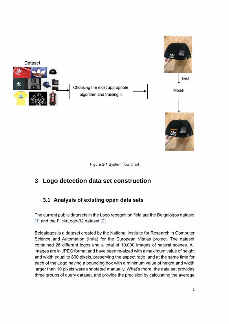
High-quality data sets are the foundation of artificial intelligence. The quality of data

sets determines the accuracy of results. The first step in this project development

process is finding the appropriate data set, then looking for the most suitable

algorithm for the requirements and data set of the project, then training the model,

and finally testing, as shown in Figure 2-1.

2

Figure 2-1 System flow chart

3 Logo detection data set construction

3.1 Analysis of existing open data sets

The current public datasets in the Logo recognition field are the Belgalogos dataset

[1] and the FlickrLogo-32 dataset [2].

Belgalogos is a dataset created by the National Institute for Research in Computer

Science and Automation (Inria) for the European Vitalas project. The dataset

contained 26 different logos and a total of 10,000 images of natural scenes. All

images are in JPEG format and have been re-sized with a maximum value of height

and width equal to 800 pixels, preserving the aspect ratio, and at the same time for

each of the Logo having a bounding box with a minimum value of height and width

larger than 10 pixels were annotated manually. What’s more, the data set provides

three groups of query dataset, and provide the precision by calculating the average

3

mAP to detect the script for the recognition effect.

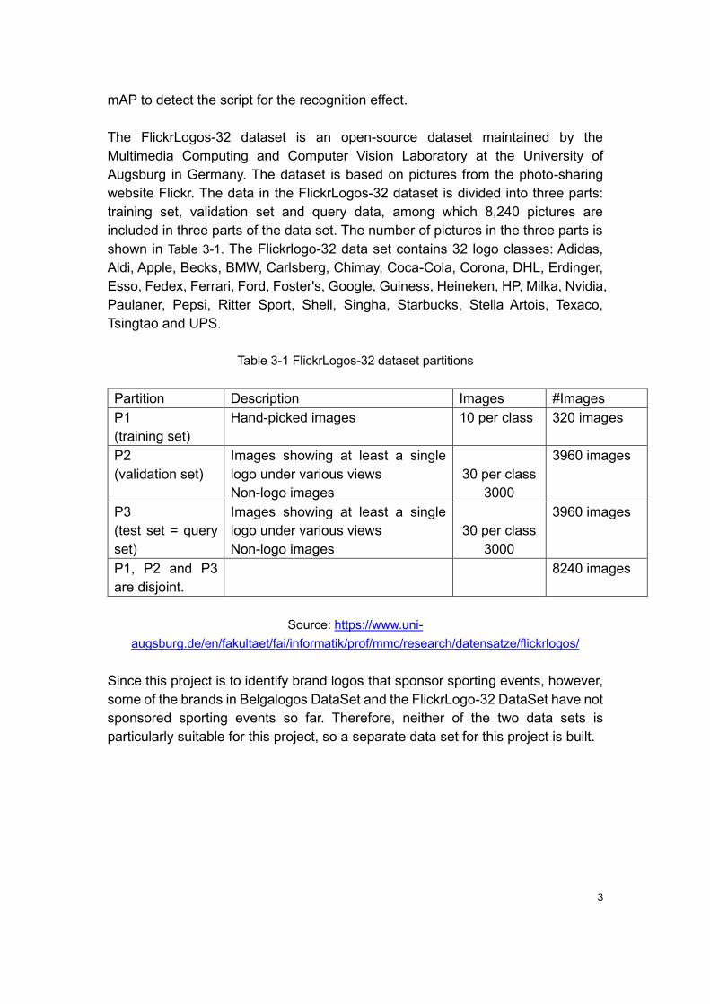
The FlickrLogos-32 dataset is an open-source dataset maintained by the

Multimedia Computing and Computer Vision Laboratory at the University of

Augsburg in Germany. The dataset is based on pictures from the photo-sharing

website Flickr. The data in the FlickrLogos-32 dataset is divided into three parts:

training set, validation set and query data, among which 8,240 pictures are

included in three parts of the data set. The number of pictures in the three parts is

shown in Table 3-1. The Flickrlogo-32 data set contains 32 logo classes: Adidas,

Aldi, Apple, Becks, BMW, Carlsberg, Chimay, Coca-Cola, Corona, DHL, Erdinger,

Esso, Fedex, Ferrari, Ford, Foster's, Google, Guiness, Heineken, HP, Milka, Nvidia,

Paulaner, Pepsi, Ritter Sport, Shell, Singha, Starbucks, Stella Artois, Texaco,

Tsingtao and UPS.

Table 3-1 FlickrLogos-32 dataset partitions

Partition Description Images #Images

P1

(training set)

Hand-picked images 10 per class 320 images

P2

(validation set)

Images showing at least a single

logo under various views

Non-logo images

30 per class

3000

3960 images

P3

(test set = query

set)

Images showing at least a single

logo under various views

Non-logo images

30 per class

3000

3960 images

P1, P2 and P3

are disjoint.

8240 images

Source: https://www.uni-

augsburg.de/en/fakultaet/fai/informatik/prof/mmc/research/datensatze/flickrlogos/

Since this project is to identify brand logos that sponsor sporting events, however,

some of the brands in Belgalogos DataSet and the FlickrLogo-32 DataSet have not

sponsored sporting events so far. Therefore, neither of the two data sets is

particularly suitable for this project, so a separate data set for this project is built.

4

3.2 Dataset collection

3.2.1 Logo type selection

This project collects 10 different logos as the data set. Selected methods were

considered through a combination of human ratings and the frequency of sporting

events sponsored. The manual rating is done by randomly selecting 10 people to

rate the collected brand impressions on a scale of 1 to 5. 1 is "never heard of", 2 is

"not very familiar", 3 is "generally", 4 is "relatively familiar" and 5 is "very familiar".

Sponsorship frequency is determined by the brand's name and sponsors of sports

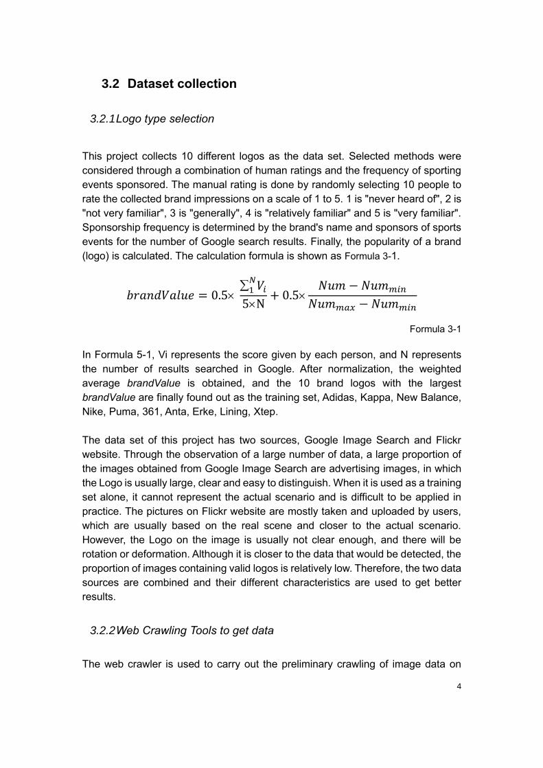
events for the number of Google search results. Finally, the popularity of a brand

(logo) is calculated. The calculation formula is shown as Formula 3-1.

𝑏𝑟𝑎𝑛𝑑𝑉𝑎𝑙𝑢𝑒 = 0.5 1

𝑁𝑉𝑖

5N+ 0.5

𝑁𝑢𝑚 − 𝑁𝑢𝑚𝑚𝑖𝑛

𝑁𝑢𝑚𝑚𝑎𝑥 − 𝑁𝑢𝑚𝑚𝑖𝑛

Formula 3-1

In Formula 5-1, Vi represents the score given by each person, and N represents

the number of results searched in Google. After normalization, the weighted

average brandValue is obtained, and the 10 brand logos with the largest

brandValue are finally found out as the training set, Adidas, Kappa, New Balance,

Nike, Puma, 361, Anta, Erke, Lining, Xtep.

The data set of this project has two sources, Google Image Search and Flickr

website. Through the observation of a large number of data, a large proportion of

the images obtained from Google Image Search are advertising images, in which

the Logo is usually large, clear and easy to distinguish. When it is used as a training

set alone, it cannot represent the actual scenario and is difficult to be applied in

practice. The pictures on Flickr website are mostly taken and uploaded by users,

which are usually based on the real scene and closer to the actual scenario.

However, the Logo on the image is usually not clear enough, and there will be

rotation or deformation. Although it is closer to the data that would be detected, the

proportion of images containing valid logos is relatively low. Therefore, the two data

sources are combined and their different characteristics are used to get better

results.

3.2.2 Web Crawling Tools to get data

The web crawler is used to carry out the preliminary crawling of image data on

5

Google Image Search and Flickr website according to the keywords. The pictures

of 10 brands are collected, 5 international brands and 5 Chinese brands, (Adidas,

Kappa, New Balance, Nike, Puma, 361, Anta, Erke, Lining, Xtep). The number of

images for each brand is shown in the Table 3-2.

Table 3-2 The number of images for each brand

Brand Number of pictures

Adidas 214

Kappa 200

New balance 201

Nike 200

Puma 204

361 200

Anta 200

Erke 191

Lining 203

Xtep 200

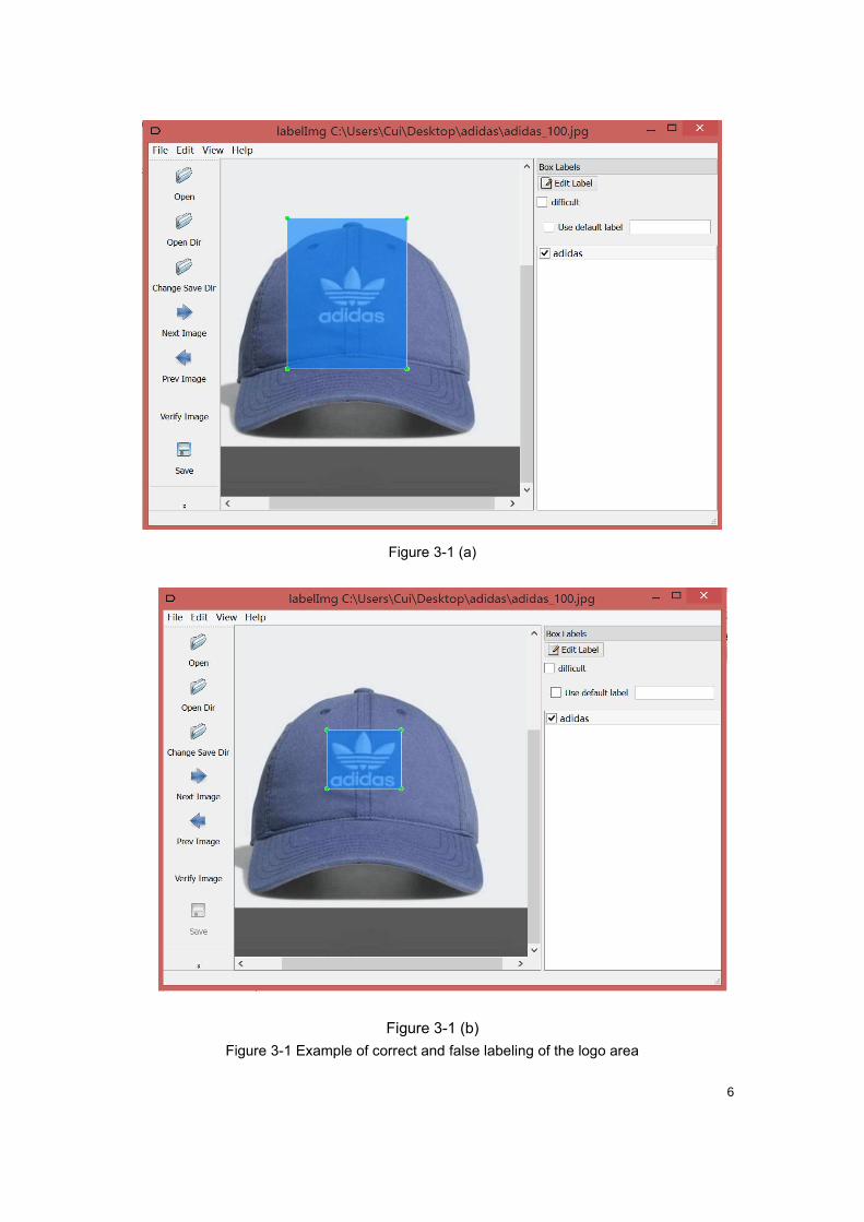
3.2.3 Manually label data

After data crawling is completed, the images obtained by the crawler should be

preliminarily screened first, and images with good quality should be selected for

labeling through labelImg, in which the labeled area of each Logo sample is a

rectangle. LabelImg generates a separate.xml file for each image, and each text

records the logo area in the sample image with (left, top, width, hight) rectangle

tagging rules. When marking the Logo manually, each area of the Logo should be

marked as accurately as possible. As shown in Figure 3-1 (a), the Logo area is too

big, which leads to the Logo in the sample area blended with other image

information, it can produce a certain amount of interference to the training of the

model, so it is a wrong labeled sample, the marked area in Figure 3-1 (b) contains

only the Logo area, does not contain other interference information, which is a

correct sample of Logo sample annotations.

6

Figure 3-1 (a)

Figure 3-1 (b)

Figure 3-1 Example of correct and false labeling of the logo area

7

The format of VOC labeled file is VOC2007 format, as shown in Figure 3-2.

Figure 3-2 VOC2007 labeling format

8

4 The parameters of performance evaluation in the

object detection

Precision, mAP and Average Precision (AP) are the main parameters to measure

the object detection algorithm.

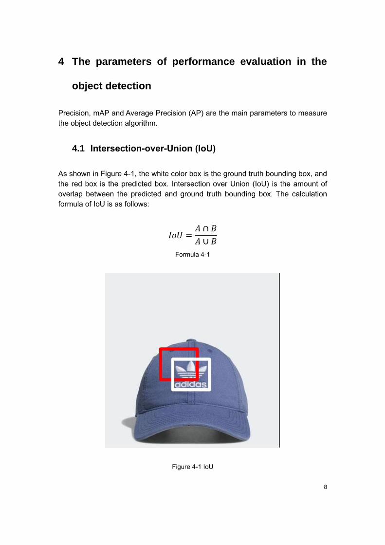
4.1 Intersection-over-Union (IoU)

As shown in Figure 4-1, the white color box is the ground truth bounding box, and

the red box is the predicted box. Intersection over Union (IoU) is the amount of

overlap between the predicted and ground truth bounding box. The calculation

formula of IoU is as follows:

𝐼𝑜𝑈 =𝐴 ∩ 𝐵

𝐴 ∪ 𝐵

Formula 4-1

Figure 4-1 IoU

9

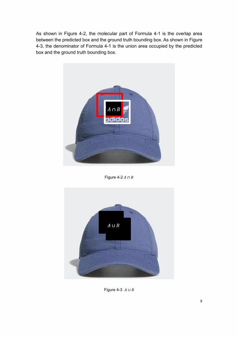
As shown in Figure 4-2, the molecular part of Formula 4-1 is the overlap area

between the predicted box and the ground truth bounding box. As shown in Figure

4-3, the denominator of Formula 4-1 is the union area occupied by the predicted

box and the ground truth bounding box.

Figure 4-2 𝐴 ∩ 𝐵

Figure 4-3 𝐴 ∪ 𝐵

10

4.2 TP TN FP FN

In a data set test, four types of test results are generated: true positive (TP), true

negative(TN), false positive (FP), false negative (FN).

T is True

F is False

P is Positive

N is Negative

T or F represents whether the sample has been correctly classified.

P or N is whether the sample is predicted to be positive or negative.

TP: Originally a positive sample, detected as a positive sample.

TN: Originally a negative sample, detected as a negative sample.

FP: Originally a negative sample, detected as a positive sample.

FN: Originally a positive sample, detected as a negative sample.

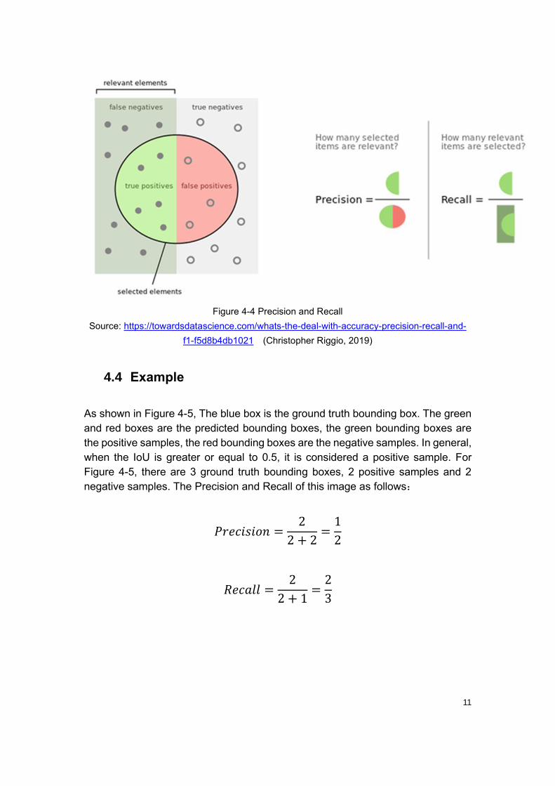
4.3 Precision and recall

Recognition accuracy is mainly represented by precision and recall. By drawing

precision-recall curve, the larger the area under the curve, the higher the

recognition accuracy, and vice versa. The precision and recall calculation formula

is shown as Formula 4-2 and Formula 4-3. Precision is the part of the positive class

detected by the classifier, and it is indeed the part of the positive class, which

accounts for the proportion of all classifiers detected to be positive. Recall is the

proportion of the part that the classifier detects that it is a positive class and is

indeed a positive class, accounting for the proportion of all that is indeed a positive

class.

𝑝𝑟𝑒𝑐𝑖𝑠𝑖𝑜𝑛 =𝑇𝑃

𝑇𝑃 + 𝐹𝑃

Formula 4-2

𝑟𝑒𝑐𝑎𝑙𝑙 =𝑇𝑃

𝑇𝑃 + 𝐹𝑁

Formula 4-3

11

Figure 4-4 Precision and Recall

Source: https://towardsdatascience.com/whats-the-deal-with-accuracy-precision-recall-and-

f1-f5d8b4db1021 (Christopher Riggio, 2019)

4.4 Example

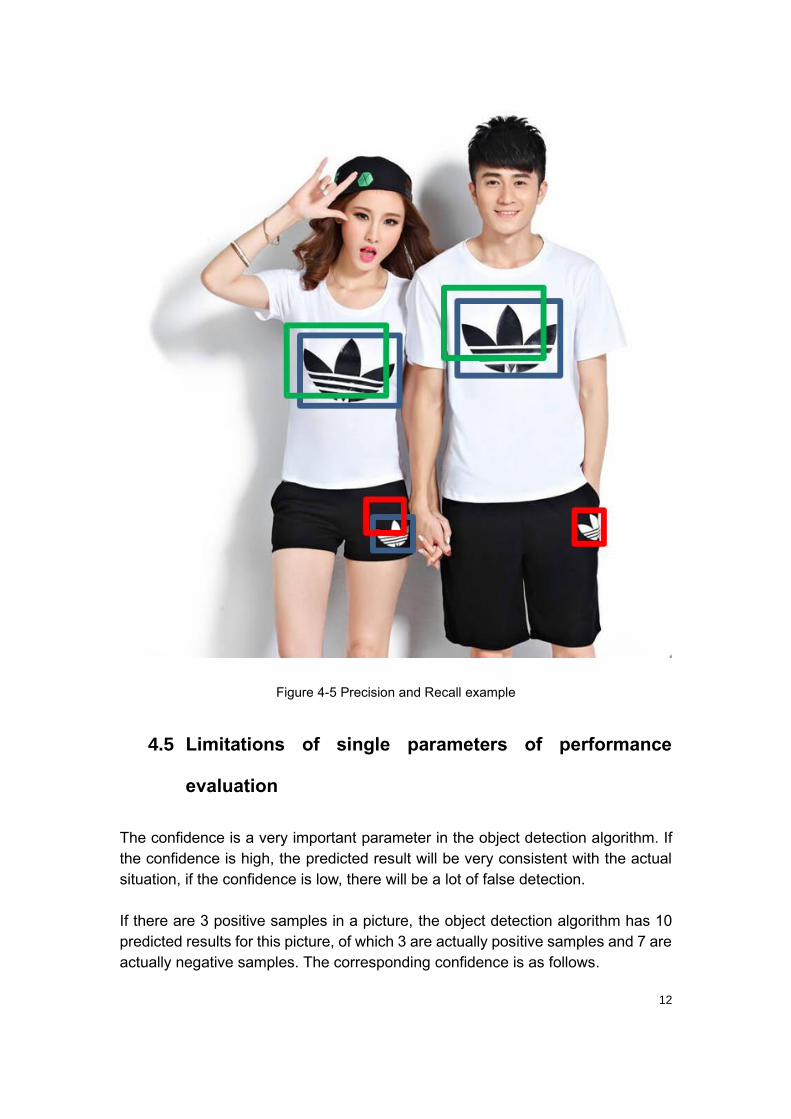
As shown in Figure 4-5, The blue box is the ground truth bounding box. The green

and red boxes are the predicted bounding boxes, the green bounding boxes are

the positive samples, the red bounding boxes are the negative samples. In general,

when the IoU is greater or equal to 0.5, it is considered a positive sample. For

Figure 4-5, there are 3 ground truth bounding boxes, 2 positive samples and 2

negative samples. The Precision and Recall of this image as follows：

𝑃𝑟𝑒𝑐𝑖𝑠𝑖𝑜𝑛 =2

2 + 2=

1

2

𝑅𝑒𝑐𝑎𝑙𝑙 =2

2 + 1=

2

3

12

Figure 4-5 Precision and Recall example

4.5 Limitations of single parameters of performance

evaluation

The confidence is a very important parameter in the object detection algorithm. If

the confidence is high, the predicted result will be very consistent with the actual

situation, if the confidence is low, there will be a lot of false detection.

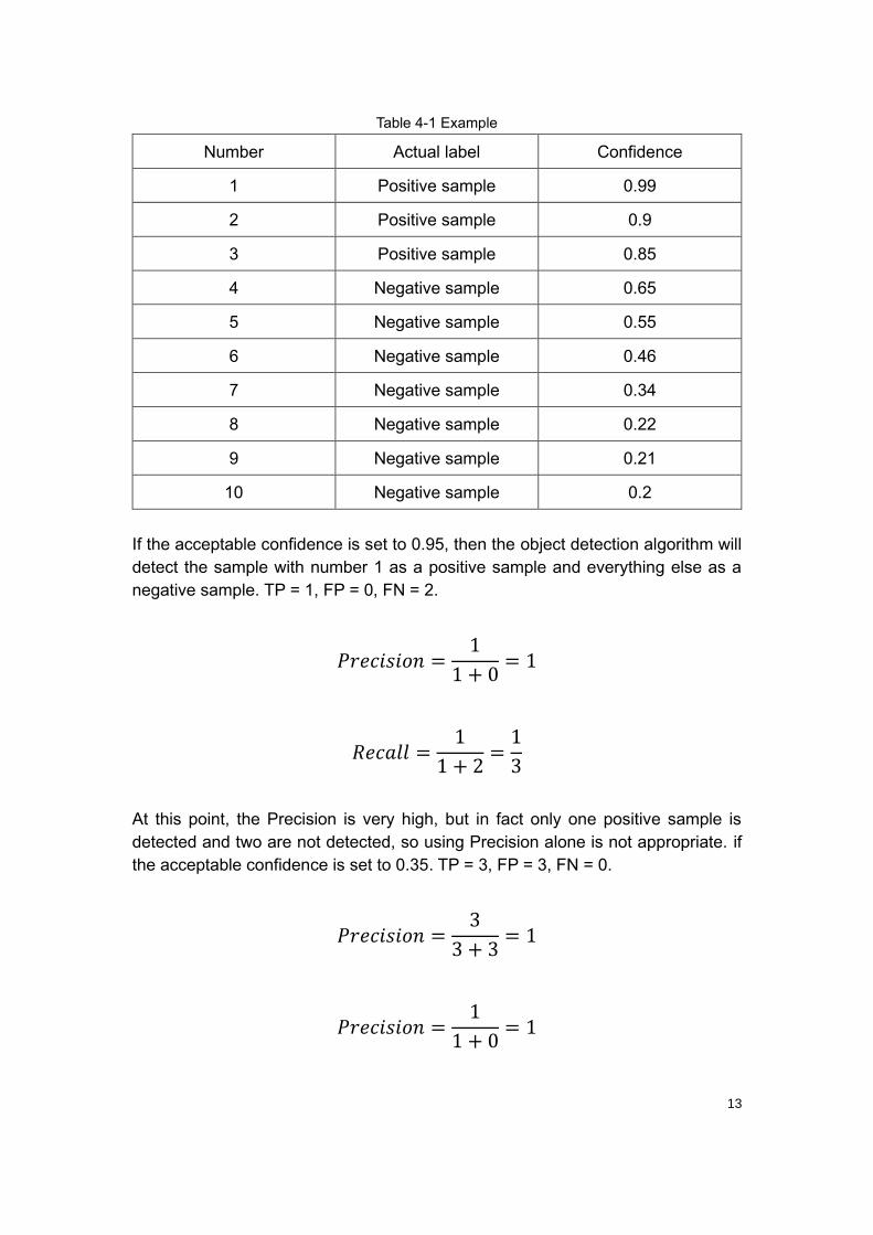
If there are 3 positive samples in a picture, the object detection algorithm has 10

predicted results for this picture, of which 3 are actually positive samples and 7 are

actually negative samples. The corresponding confidence is as follows.

13

Table 4-1 Example

Number Actual label Confidence

1 Positive sample 0.99

2 Positive sample 0.9

3 Positive sample 0.85

4 Negative sample 0.65

5 Negative sample 0.55

6 Negative sample 0.46

7 Negative sample 0.34

8 Negative sample 0.22

9 Negative sample 0.21

10 Negative sample 0.2

If the acceptable confidence is set to 0.95, then the object detection algorithm will

detect the sample with number 1 as a positive sample and everything else as a

negative sample. TP = 1, FP = 0, FN = 2.

𝑃𝑟𝑒𝑐𝑖𝑠𝑖𝑜𝑛 =1

1 + 0= 1

𝑅𝑒𝑐𝑎𝑙𝑙 =1

1 + 2=

1

3

At this point, the Precision is very high, but in fact only one positive sample is

detected and two are not detected, so using Precision alone is not appropriate. if

the acceptable confidence is set to 0.35. TP = 3, FP = 3, FN = 0.

𝑃𝑟𝑒𝑐𝑖𝑠𝑖𝑜𝑛 =3

3 + 3= 1

𝑃𝑟𝑒𝑐𝑖𝑠𝑖𝑜𝑛 =1

1 + 0= 1

14

𝑃𝑟𝑒𝑐𝑖𝑠𝑖𝑜𝑛 =3

3 + 0= 1

At this time, the Recall is very high, but in fact, among the samples detected by the

object detection algorithm as positive samples, 3 samples are indeed positive

samples, while 3 samples are negative samples. There is a very serious

misdetection, so it is not appropriate to evaluate only the Recall. A combination of

the two is the correct way to evaluate.

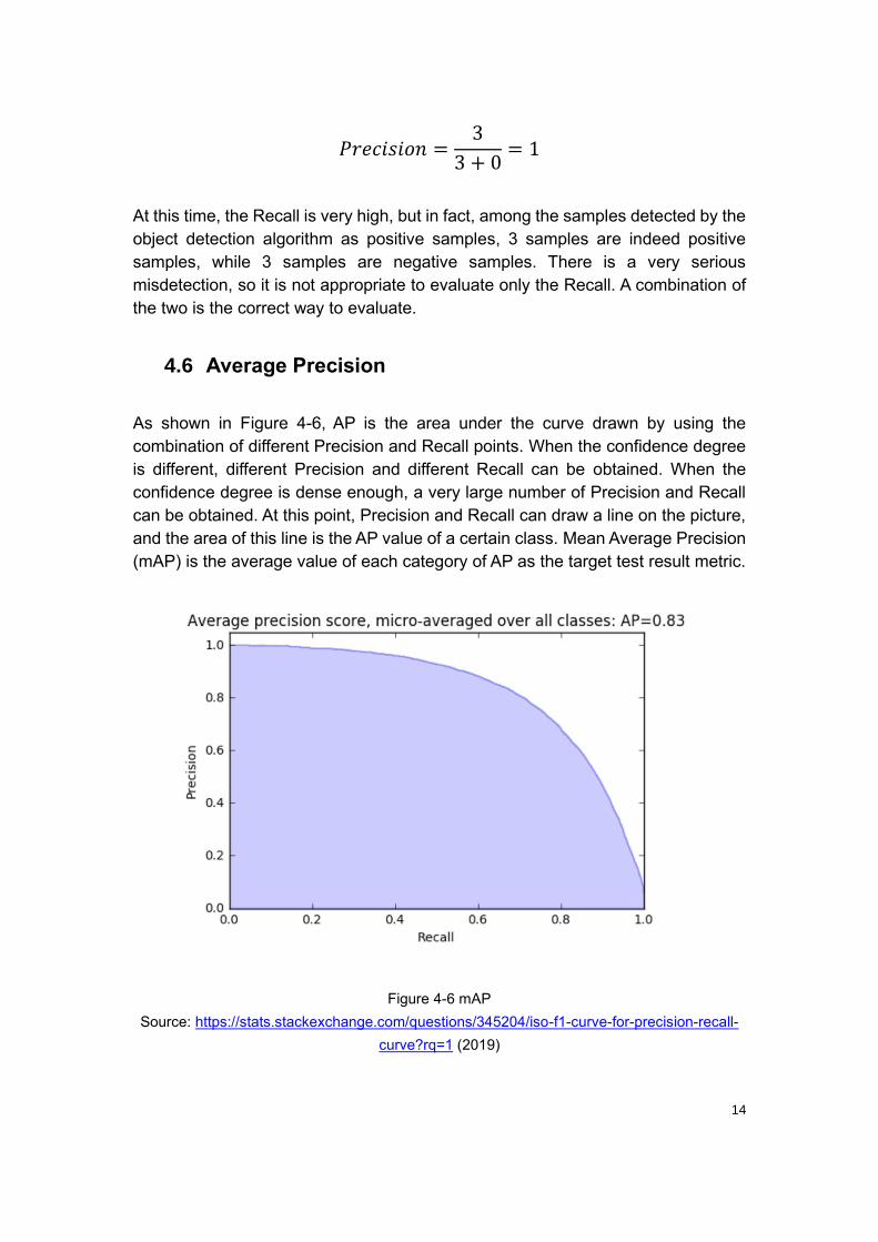
4.6 Average Precision

As shown in Figure 4-6, AP is the area under the curve drawn by using the

combination of different Precision and Recall points. When the confidence degree

is different, different Precision and different Recall can be obtained. When the

confidence degree is dense enough, a very large number of Precision and Recall

can be obtained. At this point, Precision and Recall can draw a line on the picture,

and the area of this line is the AP value of a certain class. Mean Average Precision

(mAP) is the average value of each category of AP as the target test result metric.

Figure 4-6 mAP

Source: https://stats.stackexchange.com/questions/345204/iso-f1-curve-for-precision-recall-

curve?rq=1 (2019)

15

5 Algorithms selection

In the research stage, three algorithms, Faster R-CNN, SSD and Yolov3, were

preliminarily selected. These object detection algorithms can be divided into two

categories according to their different implementation ideas:

(1) Object detection method based on candidate box. First, a large number of

candidate boxes of targets are obtained by traversal of images through sliding

windows of different scales. Then, candidate boxes are classified to obtain an

accurate target bounding box and target category. This method is called Two-Stage

object detection algorithm because it is completed in two steps: obtaining

candidate box and classifying candidate box.

(2) Object detection method based on regression, direct training network to achieve

the regression and classification of the bounding box. Because this method is

completed in one step end-to-end, it is called One-Stage object detection algorithm.

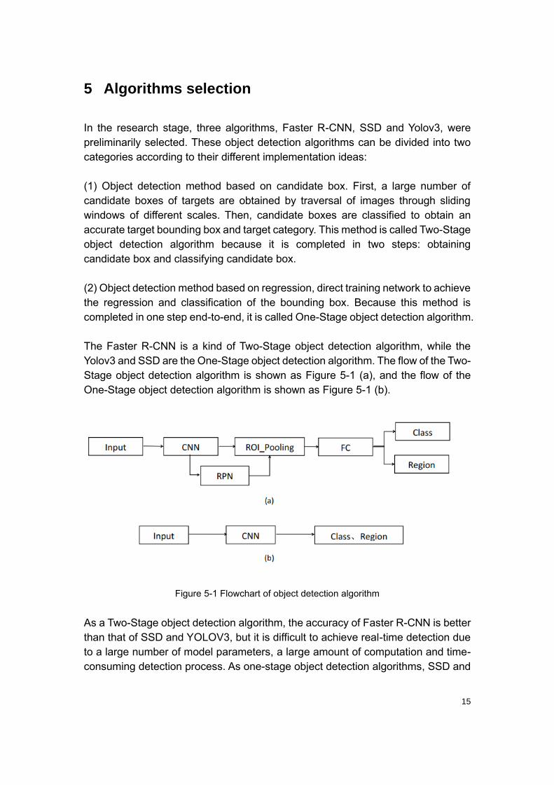
The Faster R-CNN is a kind of Two-Stage object detection algorithm, while the

Yolov3 and SSD are the One-Stage object detection algorithm. The flow of the Two-

Stage object detection algorithm is shown as Figure 5-1 (a), and the flow of the

One-Stage object detection algorithm is shown as Figure 5-1 (b).

Figure 5-1 Flowchart of object detection algorithm

As a Two-Stage object detection algorithm, the accuracy of Faster R-CNN is better

than that of SSD and YOLOV3, but it is difficult to achieve real-time detection due

to a large number of model parameters, a large amount of computation and time-

consuming detection process. As one-stage object detection algorithms, SSD and

16

Yolov3 are not as accurate as Faster R-CNN, but they have fewer model

parameters and they are faster. Table 5-1 shows the accuracy and the number of

model parameters of the above three object detection algorithms in the open-

source dataset COCO in the field of object detection.

Table 5-1 Comparison of the number of model parameters, mAP, and speed of Yolov3 SSD

Faster R-CNN in COCO dataset

Algorithm Number of parameters COCO

mAP

GPU

inference

time

CPU

inference

time

Faster-

RCNN - 0.36 198ms 720ms

SSD 26.2M 0.28 60ms 460ms

Yolov3 47.8M 0.31 38ms 230ms

6 The experimental process

This chapter will analyze the experimental process of the Faster R-CNN, SSD and

Yolov3 algorithm, find the best algorithm for detection and recognition on the Logo

dataset in this report. The environment of this experiment includes two PCs.

Without special instructions, the model training of the experiment will be completed

on PC1 by default, and the coding will be completed on PC2 by default.

Table 6-1 Laboratory environment description

PC1 PC2

operating system Windows 10 Windows 8

CPU Intel Core i7 Intel Core i5

GPU GeForce GTX 2080 None

Memory 64G 8G

6.1 Detection and recognition algorithm architecture

Logo detection and recognition is the same as most object detection and

recognition work, which is a multi-classification problem. Logo detection and

recognition based on deep learning model mainly includes two main tasks: deep

learning model training and deep learning model testing.

17

The training stage refers to the process of using data sets to train the selected

model for parameter convergence. In the test stage, the model parameters that

have been trained in the training stage are used for feature extraction, and then

the extracted features are used for classification to obtain the final output results.

In the stage of training, different network parameters and data would be used, and

then a number of different parameters for the same network model would be

obtained. The main task of the testing is loading model parameters that have been

trained, and calculating the mAP to select the best algorithm for logo detection and

recognition.

6.2 Detection and recognition method based on Faster R-

CNN

6.2.1 Introduction to the structure of Faster R-CNN

The Faster R-CNN algorithm model is shown as Figure 6-1, Fasters-RCNN can

use a variety of backbone feature extraction networks, including VGG, ResNet,

Xception, etc., and this report uses the ResNet network. Faster R-CNN does not

fix the size of the input image, but it usually fixes the short edge of the input image

to 600. If a 1200x1800 image is inputted, it will resize the image to 600x900 without

compromising the truth.

Figure 6-1 Faster R-CNN algorithm model

Source: Ren, S., He, K., Girshick, R. and Sun, J., 2015. Faster r-cnn: Towards real-time object detection with region proposal networks. arXiv preprint arXiv:1506.01497.

18

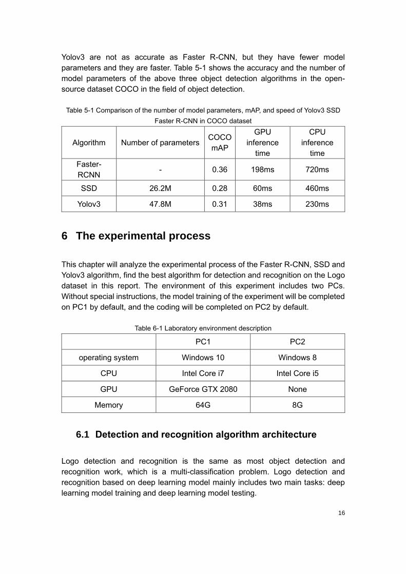
6.2.2 ResNet50

ResNet50 has two basic blocks, named Identity Block and Conv Block. The input

dimension and output dimension of Identity Block are the same. Identity Block can

be concatenated, which is used to deepen the network. The dimensions of the input

and output of Conv Block are different, so it cannot be connected continuously, and

its function is to change the dimensions of the network. The structure of Identity

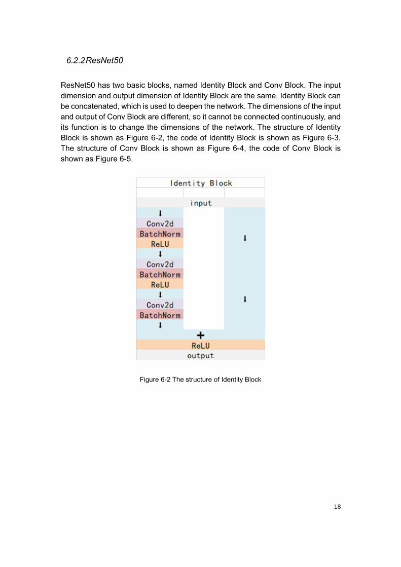
Block is shown as Figure 6-2, the code of Identity Block is shown as Figure 6-3.

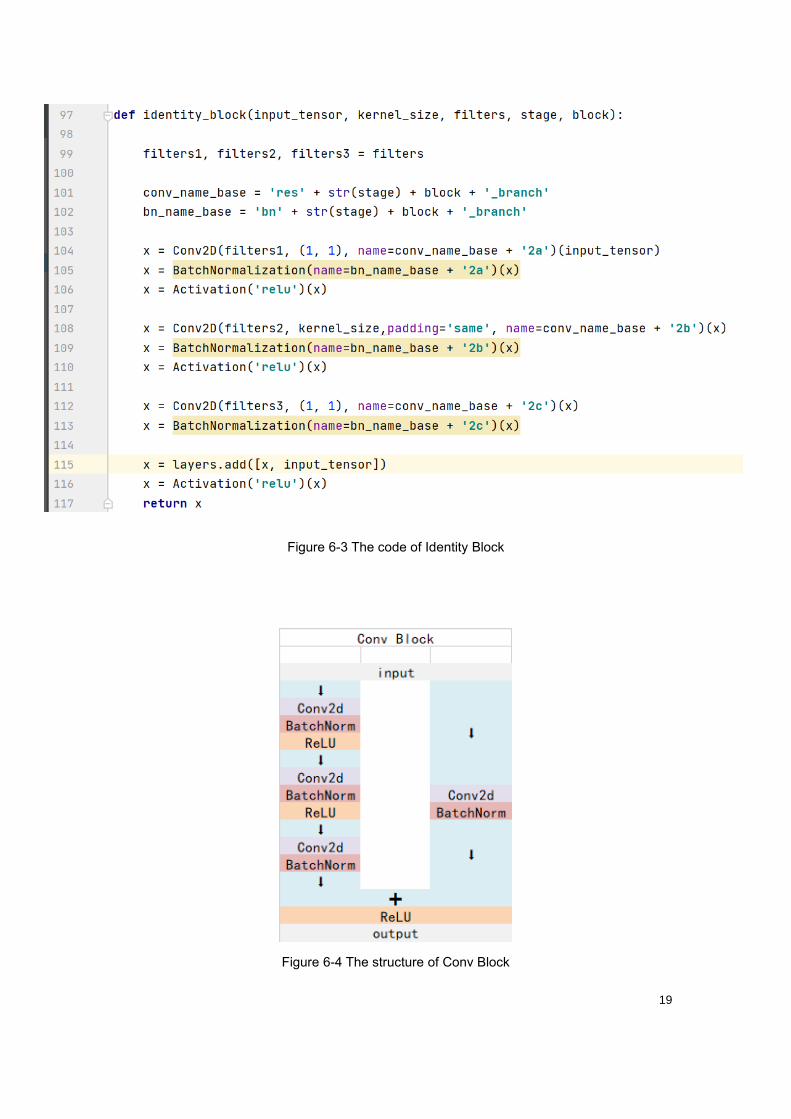
The structure of Conv Block is shown as Figure 6-4, the code of Conv Block is

shown as Figure 6-5.

Figure 6-2 The structure of Identity Block

19

Figure 6-3 The code of Identity Block

Figure 6-4 The structure of Conv Block

20

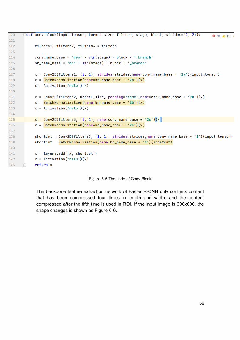
Figure 6-5 The code of Conv Block

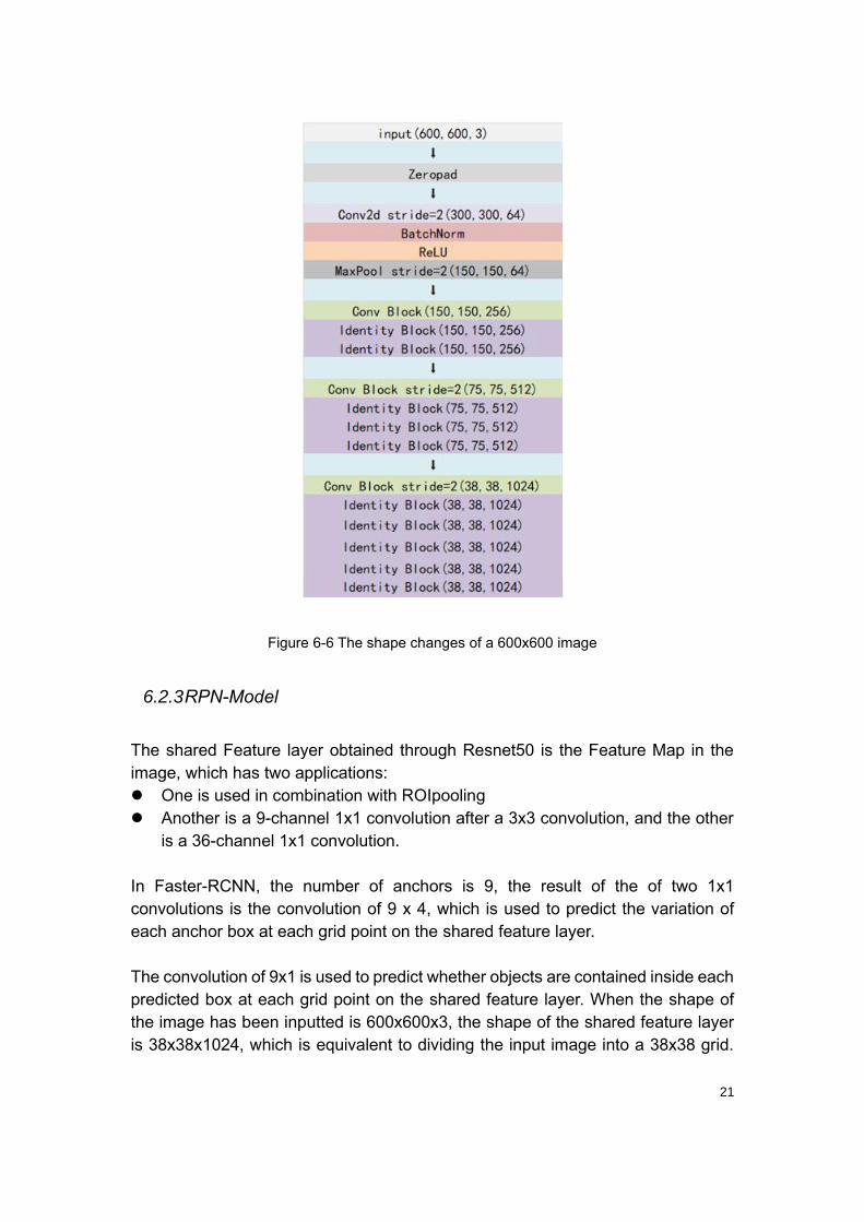
The backbone feature extraction network of Faster R-CNN only contains content

that has been compressed four times in length and width, and the content

compressed after the fifth time is used in ROI. If the input image is 600x600, the

shape changes is shown as Figure 6-6.

21

Figure 6-6 The shape changes of a 600x600 image

6.2.3 RPN-Model

The shared Feature layer obtained through Resnet50 is the Feature Map in the

image, which has two applications:

⚫ One is used in combination with ROIpooling

⚫ Another is a 9-channel 1x1 convolution after a 3x3 convolution, and the other

is a 36-channel 1x1 convolution.

In Faster-RCNN, the number of anchors is 9, the result of the of two 1x1

convolutions is the convolution of 9 x 4, which is used to predict the variation of

each anchor box at each grid point on the shared feature layer.

The convolution of 9x1 is used to predict whether objects are contained inside each

predicted box at each grid point on the shared feature layer. When the shape of

the image has been inputted is 600x600x3, the shape of the shared feature layer

is 38x38x1024, which is equivalent to dividing the input image into a 38x38 grid.

22

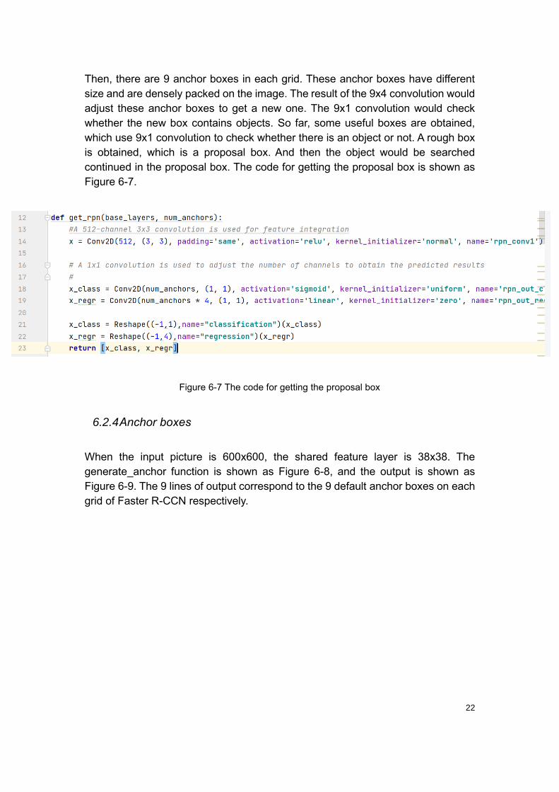
Then, there are 9 anchor boxes in each grid. These anchor boxes have different

size and are densely packed on the image. The result of the 9x4 convolution would

adjust these anchor boxes to get a new one. The 9x1 convolution would check

whether the new box contains objects. So far, some useful boxes are obtained,

which use 9x1 convolution to check whether there is an object or not. A rough box

is obtained, which is a proposal box. And then the object would be searched

continued in the proposal box. The code for getting the proposal box is shown as

Figure 6-7.

Figure 6-7 The code for getting the proposal box

6.2.4 Anchor boxes

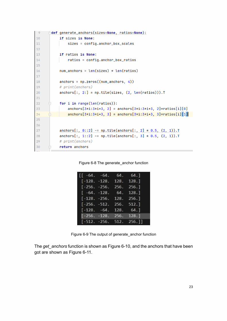
When the input picture is 600x600, the shared feature layer is 38x38. The

generate_anchor function is shown as Figure 6-8, and the output is shown as

Figure 6-9. The 9 lines of output correspond to the 9 default anchor boxes on each

grid of Faster R-CCN respectively.

23

Figure 6-8 The generate_anchor function

Figure 6-9 The output of generate_anchor function

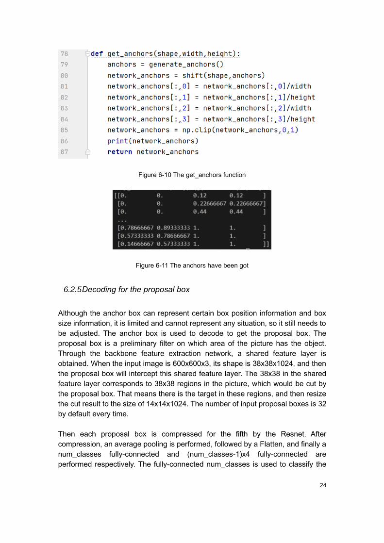
The get_anchors function is shown as Figure 6-10, and the anchors that have been

got are shown as Figure 6-11.

24

Figure 6-10 The get_anchors function

Figure 6-11 The anchors have been got

6.2.5 Decoding for the proposal box

Although the anchor box can represent certain box position information and box

size information, it is limited and cannot represent any situation, so it still needs to

be adjusted. The anchor box is used to decode to get the proposal box. The

proposal box is a preliminary filter on which area of the picture has the object.

Through the backbone feature extraction network, a shared feature layer is

obtained. When the input image is 600x600x3, its shape is 38x38x1024, and then

the proposal box will intercept this shared feature layer. The 38x38 in the shared

feature layer corresponds to 38x38 regions in the picture, which would be cut by

the proposal box. That means there is the target in these regions, and then resize

the cut result to the size of 14x14x1024. The number of input proposal boxes is 32

by default every time.

Then each proposal box is compressed for the fifth by the Resnet. After

compression, an average pooling is performed, followed by a Flatten, and finally a

num_classes fully-connected and (num_classes-1)x4 fully-connected are

performed respectively. The fully-connected num_classes is used to classify the

25

last obtained box, and fully-connected (num_classes-1)x4 is used to adjust the

corresponding proposal box.

So far, all the adjustments of the proposal box and the class of the objects in the

proposal are obtained. The adjustment proposal box is the prediction result of

Faster R-CNN, which can be drawn on the graph.

6.3 Detection and recognition method based on Single

Shot MultiBox Detector (SSD)

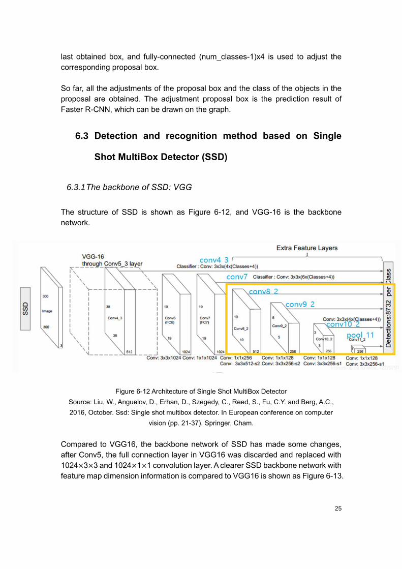
6.3.1 The backbone of SSD: VGG

The structure of SSD is shown as Figure 6-12, and VGG-16 is the backbone

network.

Figure 6-12 Architecture of Single Shot MultiBox Detector

Source: Liu, W., Anguelov, D., Erhan, D., Szegedy, C., Reed, S., Fu, C.Y. and Berg, A.C.,

2016, October. Ssd: Single shot multibox detector. In European conference on computer

vision (pp. 21-37). Springer, Cham.

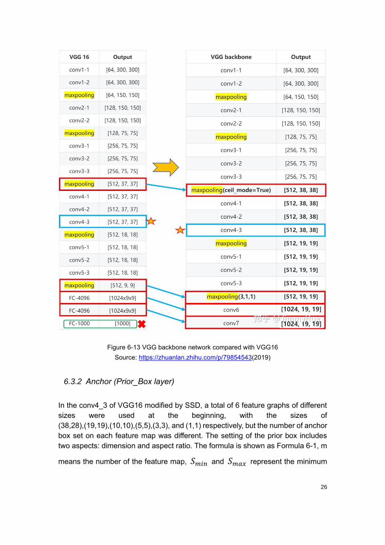
Compared to VGG16, the backbone network of SSD has made some changes,

after Conv5, the full connection layer in VGG16 was discarded and replaced with

1024×3×3 and 1024×1×1 convolution layer. A clearer SSD backbone network with

feature map dimension information is compared to VGG16 is shown as Figure 6-13.

26

Figure 6-13 VGG backbone network compared with VGG16

Source: https://zhuanlan.zhihu.com/p/79854543(2019)

6.3.2 Anchor (Prior_Box layer)

In the conv4_3 of VGG16 modified by SSD, a total of 6 feature graphs of different

sizes were used at the beginning, with the sizes of

(38,28),(19,19),(10,10),(5,5),(3,3), and (1,1) respectively, but the number of anchor

box set on each feature map was different. The setting of the prior box includes

two aspects: dimension and aspect ratio. The formula is shown as Formula 6-1, m

means the number of the feature map, 𝑆𝑚𝑖𝑛 and 𝑆𝑚𝑎𝑥 represent the minimum

27

and maximum ratio.

𝑆𝑘 = 𝑆𝑚𝑖𝑛 +𝑆𝑚𝑎𝑥 − 𝑆𝑚𝑖𝑛

𝑚 − 1(𝐾 − 1), 𝑘 ∈ [1, 𝑚]

Formula 6-1

6.3.3 The loss function of SSD algorithm

The loss function of SSD contains two parts, one is location loss and the other is classification loss. The formula of the loss function is shown in Formula 6-2, the loss function of SSD contains two parts, one is location loss and the other is

classification loss. N is the number of positive samples of the prior box, 𝑥 is the

predicted value of the network, 𝑐 is the predicted value of confidence, 𝑙 is the

predicted value of the boundary box corresponding to the prior box, 𝑔 is the

position parameter of ground truth.

𝐿(𝑥, 𝑐, 𝑙, 𝑔) =1

𝑁(𝐿𝑐𝑜𝑛𝑓(𝑥, 𝑐) + 𝛼𝐿𝑙𝑜𝑐(𝑥, 𝑙, 𝑔))

Formula 6-2

6.4 Detection and recognition method based on You only

look once (Yolov3)

6.5.1 The backbone network of Yolov3: Darknet-53

Yolov3 uses Darknet 53 (with 52 convolutional layers) as the backbone network. It

used the Residual Network method, which is setting up shortcut connections

between some layers.

28

Figure 6-14 The structure of Yolov3

Source: https://blog.csdn.net/leviopku/article/details/82660381(2018)

Figure 6-15 Darknet-53

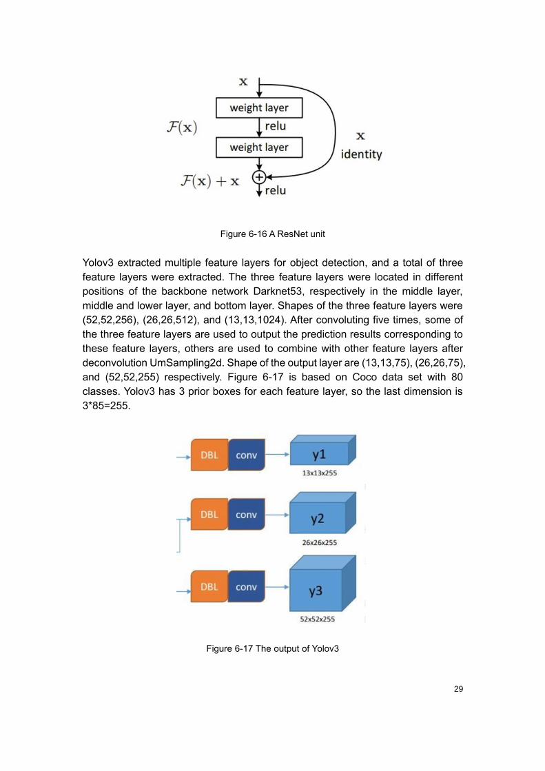
The input of the Darknet-53 network is 256*256*3. In Figure 6-15, the 1, 2, 8, and

4 in the leftmost column represent the number of duplicate ResNet units. Each

ResNet unit has two convolution layers and a shortcut connection, as shown in

Figure 6-16.

29

Figure 6-16 A ResNet unit

Yolov3 extracted multiple feature layers for object detection, and a total of three

feature layers were extracted. The three feature layers were located in different

positions of the backbone network Darknet53, respectively in the middle layer,

middle and lower layer, and bottom layer. Shapes of the three feature layers were

(52,52,256), (26,26,512), and (13,13,1024). After convoluting five times, some of

the three feature layers are used to output the prediction results corresponding to

these feature layers, others are used to combine with other feature layers after

deconvolution UmSampling2d. Shape of the output layer are (13,13,75), (26,26,75),

and (52,52,255) respectively. Figure 6-17 is based on Coco data set with 80

classes. Yolov3 has 3 prior boxes for each feature layer, so the last dimension is

3*85=255.

Figure 6-17 The output of Yolov3

30

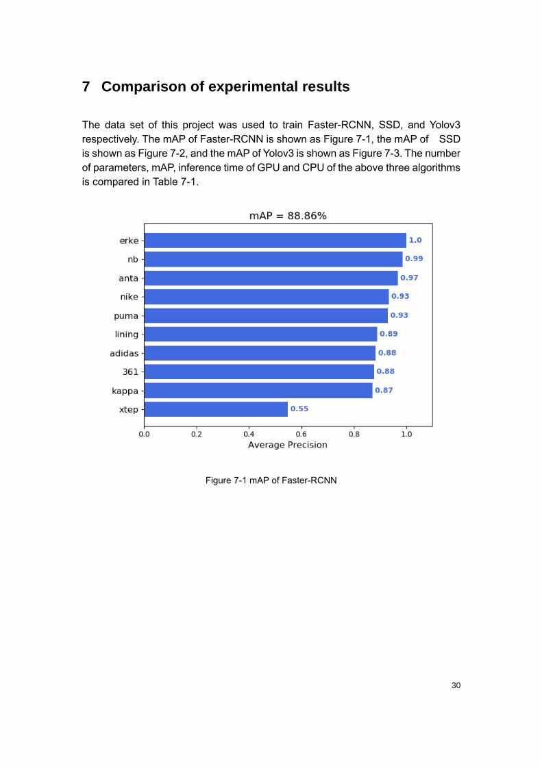
7 Comparison of experimental results

The data set of this project was used to train Faster-RCNN, SSD, and Yolov3

respectively. The mAP of Faster-RCNN is shown as Figure 7-1, the mAP of SSD

is shown as Figure 7-2, and the mAP of Yolov3 is shown as Figure 7-3. The number

of parameters, mAP, inference time of GPU and CPU of the above three algorithms

is compared in Table 7-1.

Figure 7-1 mAP of Faster-RCNN

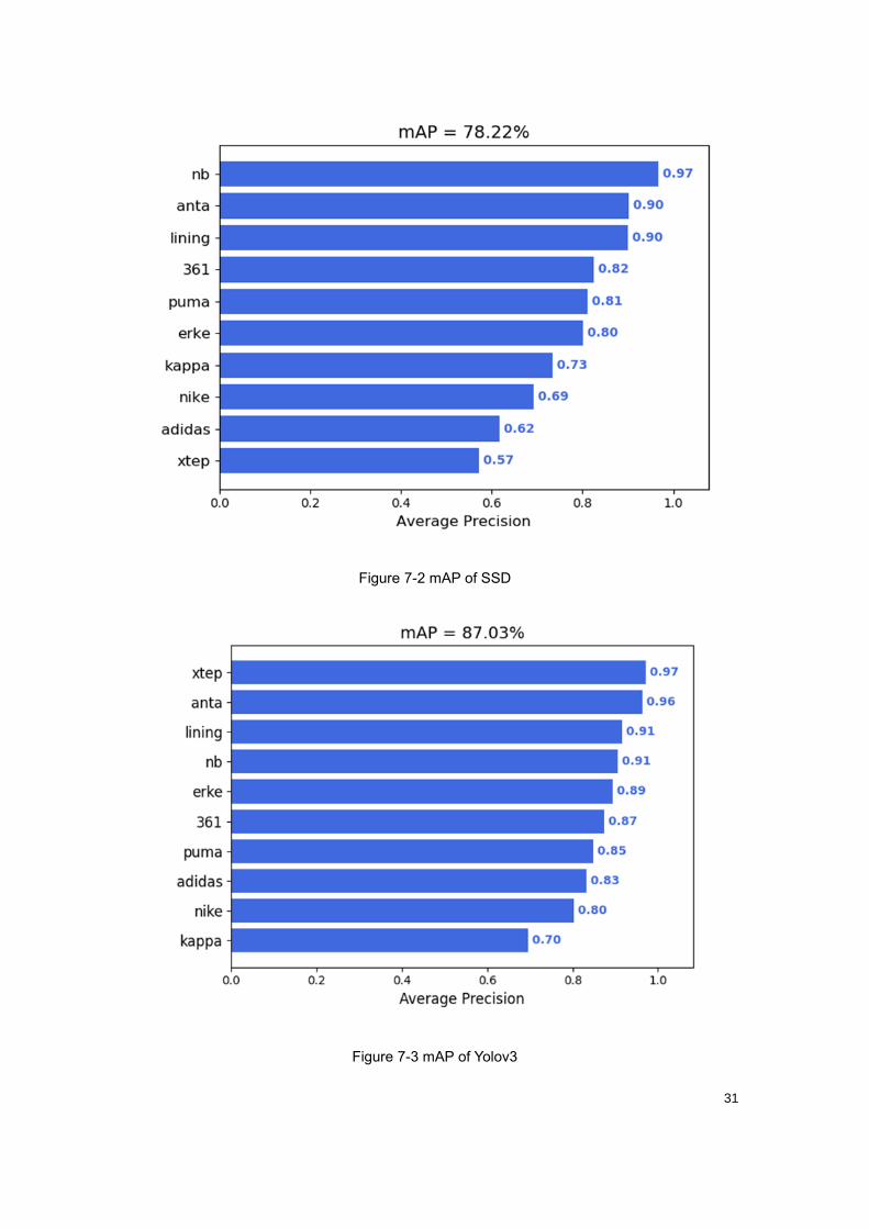
31

Figure 7-2 mAP of SSD

Figure 7-3 mAP of Yolov3

32

Table 7-1 Comparison of the number of model parameters, mAP, and speed of Yolov3 SSD

Faster R-CNN in this project dataset

Algorithm Number of parameters mAP

GPU

inference

time

CPU

inference

time

Faster-

RCNN - 0.8886 198ms 720ms

SSD 26.2M 0.7822 60ms 460ms

Yolov3 47.8M 0.8703 38ms 230ms

According to Table 7-1, Faster R-CNN has the highest accuracy, but its inference

time is too long. And the goal of this project is to detect the logos in pictures and

videos, the amount of calculation will be larger during video detection, which will

also lead to too long calculation time, so the Faster R-CNN algorithm is not chosen.

Compared with SSD and YOLOV3 in terms of accuracy, both of them meet the

requirements of detection accuracy, while YOLOV3 has advantages both in

detection accuracy and speed. After comprehensive consideration, YOLOV3 was

selected as the LOGO detection algorithm of this project.

8 Video detection

This project uses the VideoCapture Class in OpenCV to capture video.

Capture_frame.read() function reads the video by frame, ret and frame is the two

return values of the Capture_frame.read() method. Ret is a Boolean value that

returns True if the reading frame is correct and False if the file is read to the end.

A frame is an image of each frame, which is a three-dimensional matrix. Then

detect each frame from the video stream, the logos in the video is identified. The

code is as follows:

yolo_net = YOLO()

capture_frame = cv2.VideoCapture("img/ai1.mp4")

fourcc_format = cv2.VideoWriter_fourcc(*'XVID')

output_frame = cv2.VideoWriter('output.avi',fourcc_format, 24.0, (600,6

00))

frames_per_second = 0.0

while (True):

33

time1 = time.time()

ref, frame = capture_frame.read()

if ref == True:

frame = cv2.cvtColor(frame, cv2.COLOR_BGR2RGB)

frame = Image.fromarray(np.uint8(frame))

im, img = yolo_net.detecter_images(frame)

frame = np.array(img)

frame = cv2.cvtColor(frame, cv2.COLOR_RGB2BGR)

frame = cv2.resize(frame,(600,600))

frames_per_second = (frames_per_second + (1. / (time.time() - t

ime1))) / 2

print("frames_per_second= %.2f" % (frames_per_second))

frame = cv2.putText(frame, "frames_per_second= %.2f" % (frames_

per_second), (0, 40), cv2.FONT_HERSHEY_SIMPLEX, 1, (0, 0, 244), 1)

output_frame.write(frame)

cv2.imshow("aaaa", frame)

keys = cv2.waitKey(1) & 0xff

if keys == 27:

capture_frame.release()

break

else:

break

capture_frame.release()

yolo_net.close_session()

cv2.destroyAllWindows()

brands_list = (yolo_net.band_dict[k]//24.0 for k in yolo_net.band_dict.

keys())

brands_list = list(brands_list)

window = tk.Tk()

window.title('Times')

window.geometry('400x600')

Label(text='361:{}\n'

'adidas:{}\n'

'anta:{}\n'

'erke:{}\n'

'kappa:{}\n'

'lining:{}\n'

34

'nb:{}\n'

'nike:{}\n'

'puma:{}\n'

'xtep:{}\n'.format(brands_list[0],brands_list[1],brands_list

[2],brands_list[3],brands_list[4],brands_list[5],brands_list[6],brands_

list[7],brands_list[8],brands_list[9])

,font=('宋体',30)).pack()

tk.mainloop()

For real-time detection, change the VideoCapture() parameter to 0, which means

turning on the computer's camera, so the live video detection could be implement

in this way.

9 Calculating how long logo is visible in videos

First, a dictionary is define to store each brand and duration as the key-value pairs.

Then define a set that incrementing the logo's value by 1 every time a logo appears

in the image. Sets cannot have two items with the same value, duplicate values

will be ignored, which can help avoid the issue of double counting when multiple

identical logos appear in a picture. A second is generally considered to be 24

frames. Dividing the value of each logo in the dictionary by 24 (Frames PerSecond)

to get the length of time each logo appears in the video.

Figure 9-1 Defining a dictionary

35

Figure 9-2 Defining a set

Figure 9-3 Calculating how long the logo is visible

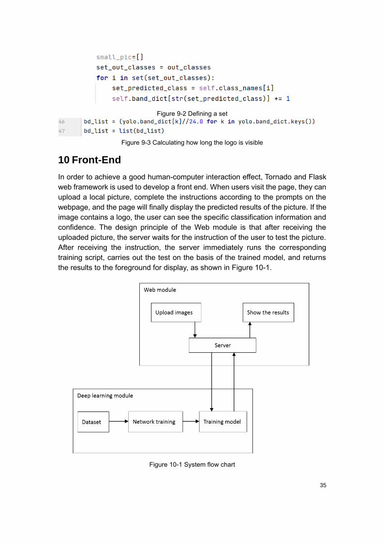
10 Front-End

In order to achieve a good human-computer interaction effect, Tornado and Flask

web framework is used to develop a front end. When users visit the page, they can

upload a local picture, complete the instructions according to the prompts on the

webpage, and the page will finally display the predicted results of the picture. If the

image contains a logo, the user can see the specific classification information and

confidence. The design principle of the Web module is that after receiving the

uploaded picture, the server waits for the instruction of the user to test the picture.

After receiving the instruction, the server immediately runs the corresponding

training script, carries out the test on the basis of the trained model, and returns

the results to the foreground for display, as shown in Figure 10-1.

Figure 10-1 System flow chart

36

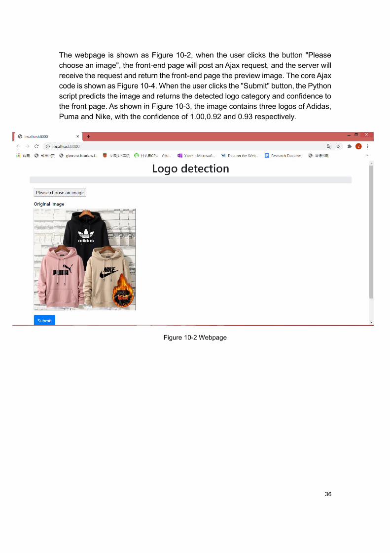
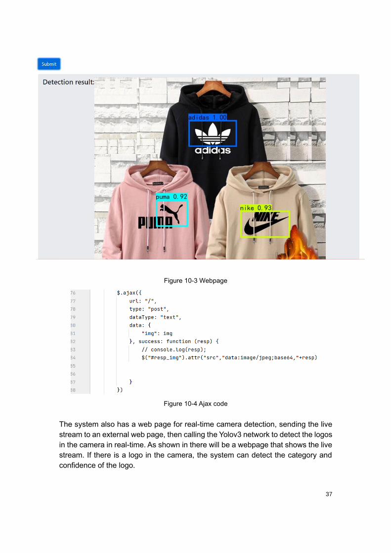
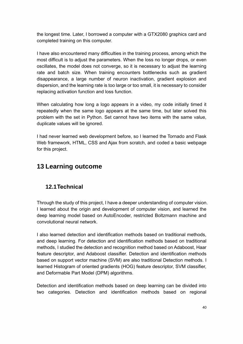
The webpage is shown as Figure 10-2, when the user clicks the button "Please

choose an image", the front-end page will post an Ajax request, and the server will

receive the request and return the front-end page the preview image. The core Ajax

code is shown as Figure 10-4. When the user clicks the "Submit" button, the Python

script predicts the image and returns the detected logo category and confidence to

the front page. As shown in Figure 10-3, the image contains three logos of Adidas,

Puma and Nike, with the confidence of 1.00,0.92 and 0.93 respectively.

Figure 10-2 Webpage

37

Figure 10-3 Webpage

Figure 10-4 Ajax code

The system also has a web page for real-time camera detection, sending the live

stream to an external web page, then calling the Yolov3 network to detect the logos

in the camera in real-time. As shown in there will be a webpage that shows the live

stream. If there is a logo in the camera, the system can detect the category and

confidence of the logo.

38

Figure 10-5 Real-time camera detection webpage

Figure 10-6 Real-time camera detection webpage

11 Locating unseen logo

Existing object detection algorithms need numerous manually labeled data. These

algorithms may misidentify the new unseen logo as a category in the data set, or

39

detect anything. In this project, the system can locate the new unseen logo in

images and videos. Template matching and Non-Maximum Suppression are used

to locate the unseen logo in this project, giving a target image of the logo, sliding

the template image (target image) over the input image, placing the template image

over the input image at any possible location, and calculating the similarity between

the template and the picture section which is overlapped. Finally, the section is

identified through Non-Maximum Suppression. As shown in Figure 4 1, the Toyota

logo isn’t trained before, the system can locate it.

Figure 11-1 Locate a logo that has never been seen before

12 Challenges

A lot of difficulties came up during the development of this project. First of all, the

training the network requires a good graphics card, but my laptop does not have

an independent graphics card, so I spent a lot of time in the training. Especially,

when training the Faster-RCNN algorithm, which has a lot of parameters, it needs

to do a large amount of computation, and training the Faster-RCNN algorithm takes

40

the longest time. Later, I borrowed a computer with a GTX2080 graphics card and

completed training on this computer.

I have also encountered many difficulties in the training process, among which the

most difficult is to adjust the parameters. When the loss no longer drops, or even

oscillates, the model does not converge, so it is necessary to adjust the learning

rate and batch size. When training encounters bottlenecks such as gradient

disappearance, a large number of neuron inactivation, gradient explosion and

dispersion, and the learning rate is too large or too small, it is necessary to consider

replacing activation function and loss function.

When calculating how long a logo appears in a video, my code initially timed it

repeatedly when the same logo appears at the same time, but later solved this

problem with the set in Python. Set cannot have two items with the same value,

duplicate values will be ignored.

I had never learned web development before, so I learned the Tornado and Flask

Web framework, HTML, CSS and Ajax from scratch, and coded a basic webpage

for this project.

13 Learning outcome

12.1 Technical

Through the study of this project, I have a deeper understanding of computer vision.

I learned about the origin and development of computer vision, and learned the

deep learning model based on AutoEncoder, restricted Boltzmann machine and

convolutional neural network.

I also learned detection and identification methods based on traditional methods,

and deep learning. For detection and identification methods based on traditional

methods, I studied the detection and recognition method based on Adaboost, Haar

feature descriptor, and Adaboost classifier. Detection and identification methods

based on support vector machine (SVM) are also traditional Detection methods. I

learned Histogram of oriented gradients (HOG) feature descriptor, SVM classifier,

and Deformable Part Model (DPM) algorithms.

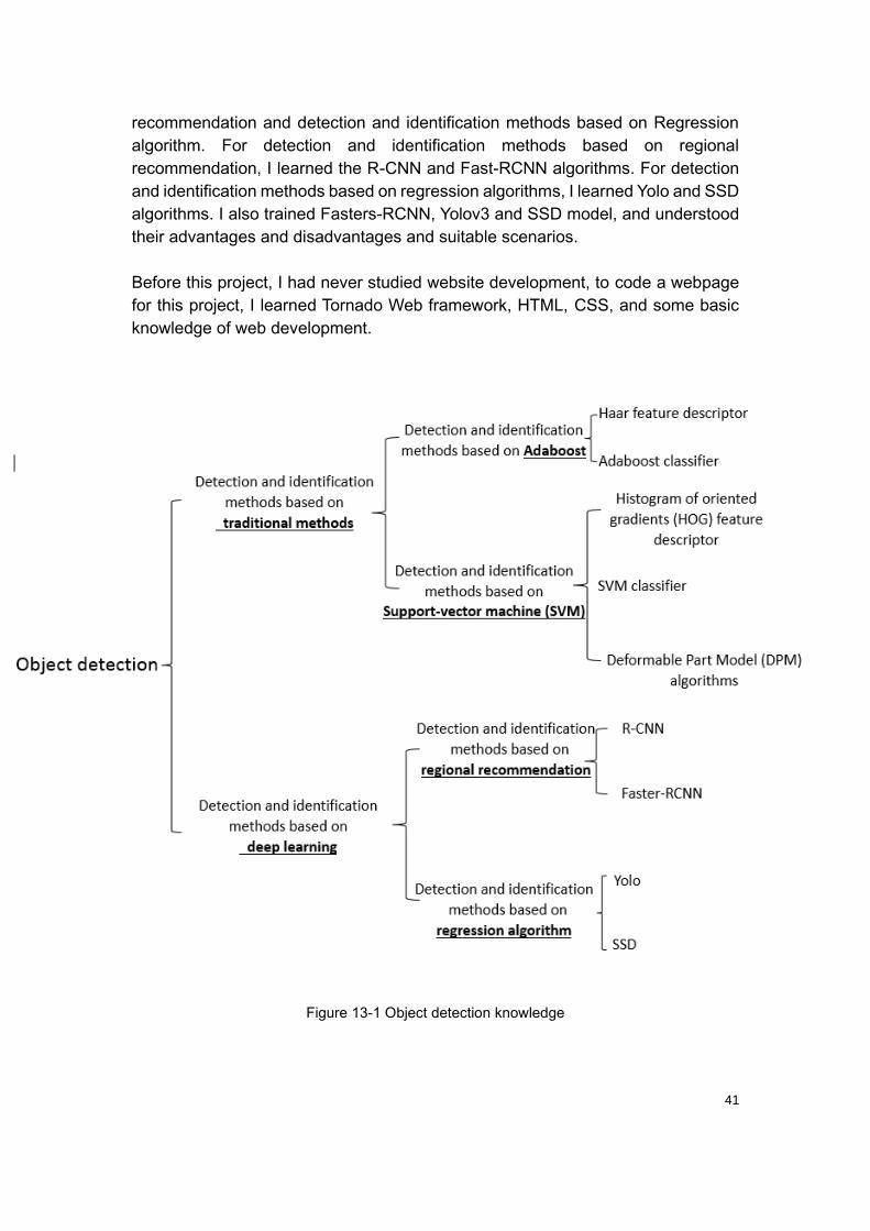
Detection and identification methods based on deep learning can be divided into

two categories. Detection and identification methods based on regional

41

recommendation and detection and identification methods based on Regression

algorithm. For detection and identification methods based on regional

recommendation, I learned the R-CNN and Fast-RCNN algorithms. For detection

and identification methods based on regression algorithms, I learned Yolo and SSD

algorithms. I also trained Fasters-RCNN, Yolov3 and SSD model, and understood

their advantages and disadvantages and suitable scenarios.

Before this project, I had never studied website development, to code a webpage

for this project, I learned Tornado Web framework, HTML, CSS, and some basic

knowledge of web development.

Figure 13-1 Object detection knowledge

42

12.2 Personal

Due to the COVID-19, this is a special year, which also is my first year in Ireland.

When I just came to Ireland last year, due to my poor English skills and the different

teaching methods, I felt very difficult to catch up. Because of the lockdown, I can't

go anywhere, just stuck at home and busy with assignments, I hardly have time to

communicate with others every day, which also makes me very anxious. I often

cried alone at night, then I tried to balance my study and life, reducing the time for

eating and sleeping, and spending more time on my study. It honed my time

management skills and sharpened my mindset. The weekly meeting also improved

my communication ability and spoken skills. I also learned about the differences

between different cultures, teachers here are more like friends.

14 Review of Project

13.1 Project summary

This project mainly aims at the insufficient performance of traditional algorithms in

logo recognition, and uses deep learning technology to preliminarily explore logo

detection, which is summarized as follows:

Traditional object detection methods usually need to manually design selected

features, carry out a large number of feature extraction operations, and finally use

a specific classifier to carry out feature classification. In contrast, the training

process of deep learning is closer to the end-to-end process, and there is no need

to pay attention to how to extract features.

This project first collected a large number of original logo images and constructed

a data set that met the requirements of this project. Then, the Faster-RCNN,SSD

and Yolov3 algorithm were adopted to identify logos, and the detection results of

the three algorithms were compared. The recognition accuracy of Faster-RCNN

was the highest, but the recognition speed was the slowest. The accuracy of SSD

is the lowest, and Yolov3, which has certain advantages in both identification

accuracy and speed, is finally selected as the algorithm of this project.

A web page based on logo recognition is designed, which mainly realizes the

function of users uploading local pictures and live stream, sending instructions, and

the server returning test results and displaying them on the page.

43

13.2 Achieved

The function of Automatic Detection of Brand Logos is as follows:

⚫ Identifying 10 different brand logos(Adidas, Kappa, New Balance, Nike, Puma,

361, Anta, Erke, Lining, Xtep) in still and moving images, and calculate how

long the logo is visible.

⚫ Users can detect images and live videos on the webpage.

⚫ Locating the new unseen logo. Giving the specific logo image, the system can

mark the location of the logo in the pictures and videos.

13.3 Weakness and future work

Although this project has made some achievements, there is still a lot of room for

progress. For some phenomena in the project, the weakness and future work is as

follows:

(1) The covered logo types in the dataset used in this project is not various enough,

and the dataset is not large enough, so the accuracy could be further improved.

It is necessary to further collect more logo pictures, or adopt effective data

expansion methods, such as affine transformation and image synthesis, to

expand the data set.

(2) Yolov3 is not very effective for detecting small objects. If I have more time, I

will try more algorithms.

(3) For logos in the fabric, it might get a ruffled appearance, the system is not very

effective for logos printed on fabric slightly stretched walked.

(4) Template matching requires high similarity between the target image and the

input image, such as brightness, gradation, angle, perspective, distance, lens,

day and night-light. For unseen logo location, I have researched open set

recognition, One-shot learning, and Few-shot learning. I have also read some

good papers and open-source code. But time is so tight, I chose the easier

way to locate the unseen logos. At first, I tried the image hashing algorithm to

compare the similarity between the target image and the input image, it can’t

locate the new logo well.

44

(5) In the research stage, the OCR technology has been tried, but OCR

technology can only recognize text and numbers, not every logo has text or

numbers, then OCR technology is given up. If the deep learning algorithm can

be combined with OCR technology, the accuracy is likely to be improved.

(6) I have never been involved in website development before. As for the timing

function of video detection, when the system is running on local computer,

there will be a window showing how long the logo is visible after the video is

processed. But when the system running on the server-side, the logo is

detected on the server-side, how to listen the video processing is completed

and then pop up a window.

45

Acknowledgements

First of all, I have to thank my supervisor, Paul Barry, for his meticulous care for my

study and life and his good guidance for my academic research. He is like a beacon,

guiding me to move forward from the darkness, making me clear from the

confusion at the beginning. He always explains to me patiently and encourages

me. I couldn't have made it through this difficult year without him.

I would like to express my gratitude to all lectures and colleagues, thanks a million

for the help and care. This year spent with them will be the best memory in my life.

Finally, I would like to thank my family in China for their love and support.

46

References

[1] Joly, A. and Buisson, O., 2009, October. Logo retrieval with a contrario visual

query expansion. In Proceedings of the 17th ACM international conference on

Multimedia (pp. 581-584).

[2] Romberg, S., Pueyo, L.G., Lienhart, R. and Van Zwol, R., 2011, April. Scalable

logo recognition in real-world images. In Proceedings of the 1st ACM

International Conference on Multimedia Retrieval (pp. 1-8).

[3] Ren, S., He, K., Girshick, R. and Sun, J., 2015. Faster r-cnn: Towards real-time

object detection with region proposal networks. arXiv preprint

arXiv:1506.01497.

[4] Liu, W., Anguelov, D., Erhan, D., Szegedy, C., Reed, S., Fu, C.Y. and Berg,

A.C., 2016, October. Ssd: Single shot multibox detector. In European

conference on computer vision (pp. 21-37). Springer, Cham.

[5] Redmon, J. and Farhadi, A., 2018. Yolov3: An incremental improvement. arXiv

preprint arXiv:1804.02767.