automatic detection of honeybees in a hive
TRANSCRIPT

IT 13 060
Examensarbete 30 hpSeptember 2013
Automatic detection of honeybees in a hive
Mihai Iulian Florea
Institutionen för informationsteknologiDepartment of Information Technology

Teknisk- naturvetenskaplig fakultet UTH-enheten Besöksadress: Ångströmlaboratoriet Lägerhyddsvägen 1 Hus 4, Plan 0 Postadress: Box 536 751 21 Uppsala Telefon: 018 – 471 30 03 Telefax: 018 – 471 30 00 Hemsida: http://www.teknat.uu.se/student
Abstract
Automatic detection of honeybees in a hive
Mihai Iulian Florea
The complex social structure of the honey bee hive has been the subject of inquirysince the dawn of science. Studying bee interaction patterns could not only advancesociology but find applications in epidemiology as well. Data on bee society remainsscarce to this day as no study has managed to comprehensively catalogue allinteractions among bees within a single hive. This work aims at developingmethodologies for fully automatic tracking of bees and their interactions in infraredvideo footage.
H.264 video encoding was investigated as a means of reducing digital video storagerequirements. It has been shown that two orders of magnitude compression ratiosare attainable while preserving almost all information relevant to tracking.
The video images contained bees with custom tags mounted on their thoraxeswalking on a hive frame. The hive cells have strong features that impede beedetection. Various means of background removal were studied, with the median overone hour found to be the most effective for both bee limb and tag detection. K-meansclustering of local textures shows promise as an edge filtering stage for limbdetection.
Several tag detection systems were tested: a Laplacian of Gaussian local maxima basedsystem, the same improved with either support vector machines or multilayerperceptrons, and the Viola-Jones object detection framework. In particular, this workincludes a comprehensive description of the Viola-Jones boosted cascade with a levelof detail not currently found in literature. The Viola-Jones system proved tooutperform all others in terms of accuracy. All systems have been found to run inreal-time on year 2013 consumer grade computing hardware. A two orders ofmagnitude file size reduction was not found to noticeably reduce the accuracy of anytested system.
Tryckt av: Reprocentralen ITCIT 13 060Examinator: Ivan ChristoffÄmnesgranskare: Anders BrunHandledare: Cris Luengo

Contents
Abbreviations vii
1 Introduction 1
2 Materials 32.1 Bee Hive . . . . . . . . . . . . . . . . . . . . . . . . . . . . . . . . 3
2.1.1 Tags . . . . . . . . . . . . . . . . . . . . . . . . . . . . . . 32.2 Video . . . . . . . . . . . . . . . . . . . . . . . . . . . . . . . . . 4
2.2.1 Video Files . . . . . . . . . . . . . . . . . . . . . . . . . . 42.3 Frame Dataset . . . . . . . . . . . . . . . . . . . . . . . . . . . . 72.4 Computing environment . . . . . . . . . . . . . . . . . . . . . . . 9
3 Video Preprocessing 103.1 Video compression . . . . . . . . . . . . . . . . . . . . . . . . . . 10
3.1.1 Cropping . . . . . . . . . . . . . . . . . . . . . . . . . . . 103.1.2 Huffman YUV . . . . . . . . . . . . . . . . . . . . . . . . 113.1.3 H.264/AVC . . . . . . . . . . . . . . . . . . . . . . . . . . 113.1.4 x264 performance . . . . . . . . . . . . . . . . . . . . . . . 15
3.2 Background removal . . . . . . . . . . . . . . . . . . . . . . . . . 233.2.1 Clustering . . . . . . . . . . . . . . . . . . . . . . . . . . . 253.2.2 Frame differencing . . . . . . . . . . . . . . . . . . . . . . 323.2.3 Exponentially weighted moving average . . . . . . . . . . 323.2.4 True average . . . . . . . . . . . . . . . . . . . . . . . . . 363.2.5 Histogram peak . . . . . . . . . . . . . . . . . . . . . . . . 363.2.6 Percentile . . . . . . . . . . . . . . . . . . . . . . . . . . . 373.2.7 Mixture of Gaussians . . . . . . . . . . . . . . . . . . . . . 39
3.3 Discussion and future work . . . . . . . . . . . . . . . . . . . . . 43
4 Tag detection 454.1 Why is tag detection difficult? . . . . . . . . . . . . . . . . . . . . 454.2 LoG pipeline . . . . . . . . . . . . . . . . . . . . . . . . . . . . . 474.3 Viola-Jones object detection framework . . . . . . . . . . . . . . 52
4.3.1 Haar-like Features . . . . . . . . . . . . . . . . . . . . . . 524.3.2 Adaboost . . . . . . . . . . . . . . . . . . . . . . . . . . . 564.3.3 Boosted cascade . . . . . . . . . . . . . . . . . . . . . . . 634.3.4 Results . . . . . . . . . . . . . . . . . . . . . . . . . . . . 71
4.4 Benchmarks . . . . . . . . . . . . . . . . . . . . . . . . . . . . . . 744.4.1 Multilayer perceptrons . . . . . . . . . . . . . . . . . . . . 74
v

4.4.2 Support vector machines . . . . . . . . . . . . . . . . . . . 744.4.3 Benchmark training dataset . . . . . . . . . . . . . . . . . 75
4.5 Results . . . . . . . . . . . . . . . . . . . . . . . . . . . . . . . . . 804.5.1 Multilayer perceptrons . . . . . . . . . . . . . . . . . . . . 814.5.2 Support vector machines . . . . . . . . . . . . . . . . . . . 834.5.3 Effect of compression on performance . . . . . . . . . . . 844.5.4 Average running times . . . . . . . . . . . . . . . . . . . . 88
5 Discussion and future work 905.1 Background removal . . . . . . . . . . . . . . . . . . . . . . . . . 905.2 Tag detection . . . . . . . . . . . . . . . . . . . . . . . . . . . . . 905.3 Future experiments . . . . . . . . . . . . . . . . . . . . . . . . . . 91
6 Conclusions 93
Bibliography 95
A Video transcoding 99
B Improving the custom tags through ID choice 101
vi
Abbreviations
AFPT Average Frame Processing Time
ARTag Augmented Reality Tag
AVC Advanced Video Coding
B-frame Bidirectional frame
BMB B-frame Macroblock
CPU Central Processing Unit
DCT Discrete Cosine Transform
DDR Double Data Rate
DPCM Differential Pulse Code Modulation
DVQ Digital Video Quality
EWMA Exponentially Weighted Moving Average
FFMPEG Fast Forward Moving Picture Experts Group
fn false negative count
fp false positive count
FPR False Positive Rate
fps frames per second
GCC GNU Compiler Collection
GiB Gibibyte (1073741824 bytes)
GNU GNU’s Not Unix (recursive acronym)
GPL General Public License
HDD Hard Disk Drive
I-frame Intra-coded frame
iDCT inverse Discrete Cosine Transform
JDD Just Noticeable Difference
vii

kB kilobyte (1000 bytes)
KiB Kibibyte (1024 bytes)
LED Light-Emitting Diode
LoG Laplacian of Gaussian
MB Macroblock
MB Megabyte (1000000 bytes)
MLC Multi-Level Cell
MLP Multilayer Perceptrons
MNIST Mixed National Institute of Standards and Tech-nology dataset
MOG Mixture of Gaussians
MPEG Moving Picture Experts Group
MSE Mean Squared Error
OpenCV Open Source Computer Vision Library
P-frame Predicted frame
PMB P-frame Macroblock
QP Quantization Parameter
RAM Random-Access Memory
RANSAC Random Sample Consensus
RBFNN Radial Basis Function Neural Network
RGB Red Green Blue
ROC curve Receiver Operating Characteristic curve
RPM Revolutions Per Minute
RProp Resilient Propagation
SATA Serial Advanced Technology Attachment
SSD Solid-State Drive
SSIM Structural Similarity
SVM Support Vector Machine
tn true negative count
tp true positive count
TPR True Positive Rate
viii

VCR Video Cassette Recording
YCrCb Luma (Y), Chrominance red (Cr) and Chromi-nance blue (Cb) color space
YUV Color space made up of a luma (Y) and twochrominance components (UV)
ix
Chapter 1
Introduction
Honey bees (Apis mellifera) exhibit many forms of intelligent behavior beingthe only species, apart from humans, that are able to communicate directions[1]. Given their complex social structure, where individuals have clearly definedroles, it is very likely that interactions among bees could bear resemblance withthose among humans.
Human sociological studies are limited in their effectiveness due to restric-tions in data collection methods. A bee colony on the other hand is self-contained, with few social interactions outside it. Hives can be artificially mod-ified by experimenters who may open them completely in order to observe everyinteraction. This can enable cataloging all honeybee motions and provide valu-able data to social sciences. Information on disease transmission in social groupsis of particular interest [2]
Scientific inquiry into honey bee behavior stems back to antiquity [3]. Aris-totle mentions the bee waggle dance, uncertain of its meaning. He also observedsimilarities between human and honey bee societies, grouping both species intothe category of “social animals”.
Von Frisch [1] has proven that honey bees are capable of communicating di-rections through the waggle dance. Experimentation and data collection had tobe carried out manually, which limited the accuracy and quantity of informationobtained.
More recently, computer assisted tracking of bee movements has been accom-plished [4]. Through these studies, trajectories of single bees have been automat-ically mapped from video recordings using Probabilistic Principal ComponentAnalysis for intra-frame position recognition and Rao-Blackwellized Particle Fil-ters for inter-frame trajectory prediction. Excellent results were obtained with-out the aid of any markers on the bees. However, tracking a single individualoffers little insight into communication and disease transmission.
Hundreds of bees at a time have been tracked in video sequences [5] withthe aid of large circular markers painted on their thoraxes. Unfortunately, thetrajectories extracted do not contain head orientation data that are necessaryfor the detection of trophallaxis - the transfer of food between bees by meansof their tongues [6]. Separating the camera and hive using a transparent screenallowed bees to walk on its surface, occluding the marker.
By marking both the dorsal and ventral parts of the abdomen with a largemarker, more consistent data has been obtained [7]. Again the head orientation
1
problem has not been addressed.A very ambitious study [8] has managed to devise a method for extract-
ing the posture of hundreds of bees at a time from very low resolution video.By approximating the shape of honey bee bodies by an oval of constant sizethroughout the sequence, head posture information has been inferred with areasonable degree of accuracy. The video images have been segmented usingVector Quantization (a form of clustering) and a separate post-processing stephas been employed to separate touching bees. Analysis was limited to a fewminutes of video. In addition, the hive was illuminated with red light that mayhave altered bee behavior [6].
The current work, initiated at the Department of Ecology of the SwedishUniversity of Agricultural Sciences (SLU), caters the need of developing bettermethodologies for fully automated tracking of all movements of all the bees ina single hive, including head and antennae positions.
Given the complexity of the tasks at hand, the scope of this work will belimited to achieving the following objectives:
1. Find a methodology to reduce as much as possible the size of the recordedvideo while preserving relevant details. Storing hive videos totaling sev-eral weeks in length at a resolution high enough to allow the identificationof individual bees is beyond the capability of 2013 consumer storage tech-nology. At least an order of magnitude size reduction is necessary to makelong term recording feasible at this point.
2. Determine whether it is feasible to track all the bees in real-time. Shouldthis be possible, only interaction data would need to be recorded, greatlyreducing the storage requirements.
3. All software platforms utilized in this work ought to be made entirely offree [9] or at least open source software. The availability of the code pro-vides several advantages. First and foremost, it adheres to the academicprinciple of openness. Second, it makes the methodology reproducible.And lastly, compiling source code instead of using prebuilt binaries leadsto increased performance, necessary when dealing with large amounts ofdata.
2
Chapter 2
Materials
Researchers at the SLU and Uppsala University have recorded raw video footageof bees for offline analysis with the hope that the methods developed on recordedvideo can be sped up sufficiently to allow real time analysis [2].
2.1 Bee HiveThe honey bees were filmed in a standard observation hive (width 43.5 cm,height 52.5 cm, depth 5.5 cm) containing two standard hive frames (width 37cm and height 22 cm each) mounted vertically one on top of the other. TwoPlexiglas sheets found on both sides of the hive were used to contain the bees.The hive was placed in a small, dark, windowless room and was sealed so that nobee could enter or leave the hive during filming. Bees were kept alive by drippingsugar water into the hive. To simplify the experiment, bees were marked withtags placed only on their backs. In order to prevent the bees from walking onthe screen and thus occluding their tags, the experimenters sprayed the screenwith a thin film of Fluon, a slippery coating agent, with the help of an air-brushinstrument.
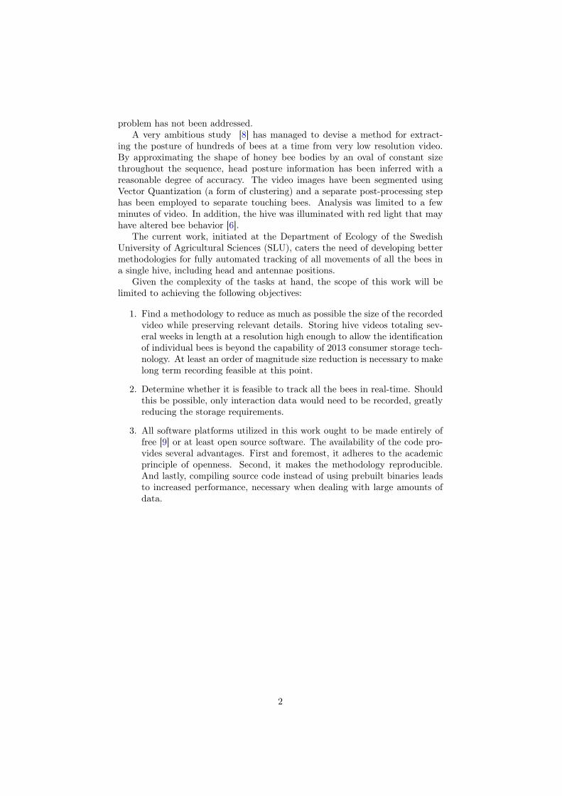
2.1.1 TagsGenerally, bee-keepers are interested in tagging only the queen of each hive.The tags they use are small, circular (of 3 mm in diameter) and inscribed withArabic numerals. This method however cannot be extrapolated to the highnumber of bees simultaneously tracked in this experiment. Consequently, aninnovative square tag design was chosen instead (fig. 2.1) [2]. The tags aresquare in shape, of size 3 mm by 3 mm. The bright white rectangle (gray level255 on a 0 to 255 scale) in the center is used in the detection of the bee. The tagis glued on the dorsal part of the thorax of the bee with the white line emergingfrom the center pointing towards the head. The 8 rectangular patches, markedc0, c1, ..., c7 are homogeneous, with the gray level encoding a base 3 digit: (0 toencode digit 0, 65 for 1, 130 for 2). The number encoded by the tag is given byc0 · 37 + c1 · 36 + ...+ c7 · 30 yielding an ID range of 0 to 6560.
3
c0
c1
c2
c3
c4
c5
c6
c7
head direc1on
Figure 2.1: The custom tag design
2.2 VideoA Basler Scout scA1600-14gm camera mounted with Fujinon HF16HA-1B lensand 850 nm bandpass filter was used to film the hive. LED lights at 850 nm wereused for illumination. Instead of employing a diffusion system, the frame waslit from a wide angle with respect to the camera, so that no specular reflectionsfrom the screen would enter the field of view. Bees are thought to be insensitiveto near infrared light [1] and should behave as if in total darkness.
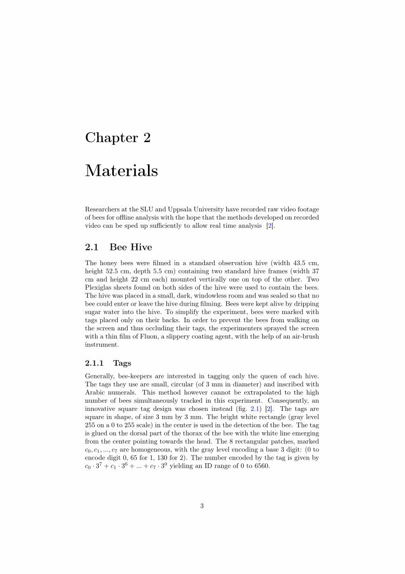
The distance between the camera and the hive frame was of 80 cm so thatthe field of view encompassed the entire frame, with a small margin. The opticalaxis is perpendicular to the center of the frame. A typical video frame is shownin fig. 2.2.
Filming took place over the course of five days. Due to limitations in hard-disk capacity, only around 11 hours of video were recorded at a time with breaksin between for computer servicing and cleaning of the glass.
The video was recorded using frames of size 1626×1236 pixels at a frequencyof 14.3 fps. The video frames contain only one 8 bit channel corresponding to850 nm near-infrared light intensity. The encoding format is lossless HuffmanYUV compression [10].
2.2.1 Video FilesThe entire video material comprises 10 files totaling around 5 continuous days offootage. The video files with their corresponding lengths are listed in Table 2.1.A detailed description of their contents is as follows:
d1_140812.avi The image is very sharp and the tags are clearly visible. Around150 live bees are present. The hive has a queen, which is surrounded bybees tending it. Sugar water drips from the top of the hive to keep thebees alive. A large number of bees lie dead at the bottom of the frame andthere are a few bodies higher up. Some bees have ripped the tags fromtheir backs and these tags, whole or in pieces, can be found in variouspoints across the frame. After 1 hour, the liquid produces splash marksin the lower part of the screen. Bees are clumped around the extremitiesof the hive initially and form two clumps in the upper part of the frametowards the end of the video.
4
Figure 2.2: A typical video frame. The size in pixels is 1626×1236. The imageis in grayscale format with one 8-bit channel. The original film was upside down.Here the frame is shown after being rotated 180◦.
d1_150812.avi The same hive as in the previous video is filmed. The queenis still present and the bees gather around it. For this reason, almost allthe bees are located in the left side of the frame while little activity canbe seen on the right side. The liquid splashes are visible from the verybeginning and remain a problem throughout the video.
d1_150812_extra.avi Almost the same as the previous video with the ex-ception that the right side of the frame has a few active bees.
d2_210812.avi A different bee hive is filmed from now on. No queen is presentand the hive is better lit than in the previous videos. The image is notvery sharp although the hive does not have debris nor dripping liquid. Inthis sequence, the bees are very inactive and form a single clump thatmoves slowly around the frame. In the end, the video looks more blurry,most likely because the breath of the bees fogs up the screen.
d2_210812_del2.avi The video starts with all bees forming a single largeclump. During the next 6 hours, the clump moves around slightly andthen splits into two less dense clumps starting from the 8th hour. Afterthe 9th hour, the bees are spread out somewhat with occasional crowding.During the first 12 hours, the bees are very stationary. Starting with the13th hour the bees start moving around.
d3_220812_del1_LON.avi For the first 3 hours, the bees move around en-
5
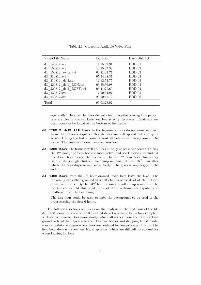
Table 2.1: Currently Available Video Files
Video File Name Duration Hard-Disk ID
d1_140812.avi 11:15:39.91 HDD 01d1_150812.avi 10:25:37.38 HDD 02d1_150812_extra.avi 00:21:33.77 HDD 02d2_210812.avi 05:34:48.37 HDD 03d2_210812_del2.avi 12:12:52.75 HDD 03d3_220812_del1_LON.avi 03:55:36.98 HDD 04d3_220812_del2_LOFF.avi 05:41:27.60 HDD 04d3_230812.avi 17:20:04.97 HDD 05d4_240812.avi 23:20:47.19 HDD 06
Total 90:08:28.92
ergetically. Because the bees do not clump together during this period,tags are clearly visible. Later on, bee activity decreases. Relatively fewdead bees can be found at the bottom of the frame.
d3_220812_del2_LOFF.avi In the beginning, bees do not move as muchas in the previous sequence though bees are well spread out and quiteactive. During the last 2 hours, almost all bees move quickly around theframe. The number of dead bees remains low.
d3_230812.avi The frame is well lit. Bees initially linger in the center. Duringthe 4th hour, the bees become more active and start moving around. Afew dozen bees escape the enclosure. In the 8th hour bees clump verytightly into a single cluster. The clump remains until the 16th hour afterwhich the bees disperse and move freely. The glass is very foggy in theend.
d4_240812.avi From the 7th hour onward, most bees leave the hive. Theremaining are either grouped in small clumps or lie dead at the bottomof the hive frame. By the 23rd hour, a single small clump remains in thetop left corner. At this point, most of the hive frame lies exposed andunaltered from the beginning.
The last hour could be used to infer the background to be used in thepreprocessing the first 6 hours.
The following sections will focus on the analysis to the first hour of the filed1_140812.avi. It is one of the 3 files that depict a realistic bee colony completewith its own queen. Bees move slowly, which allows for more accurate trackinggiven the fixed 14.3 fps framerate. The bee bodies and dripping liquid modela more realistic scenario where bees are confined for longer spans of time. Thefirst hour does not show any liquid splashes, which are difficult to account forwhen looking for tags.
6
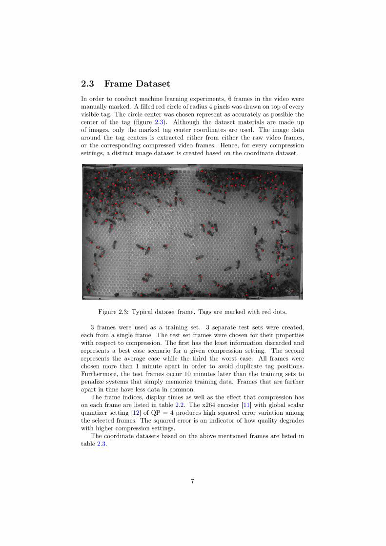
2.3 Frame DatasetIn order to conduct machine learning experiments, 6 frames in the video weremanually marked. A filled red circle of radius 4 pixels was drawn on top of everyvisible tag. The circle center was chosen represent as accurately as possible thecenter of the tag (figure 2.3). Although the dataset materials are made upof images, only the marked tag center coordinates are used. The image dataaround the tag centers is extracted either from either the raw video frames,or the corresponding compressed video frames. Hence, for every compressionsettings, a distinct image dataset is created based on the coordinate dataset.
Figure 2.3: Typical dataset frame. Tags are marked with red dots.
3 frames were used as a training set. 3 separate test sets were created,each from a single frame. The test set frames were chosen for their propertieswith respect to compression. The first has the least information discarded andrepresents a best case scenario for a given compression setting. The secondrepresents the average case while the third the worst case. All frames werechosen more than 1 minute apart in order to avoid duplicate tag positions.Furthermore, the test frames occur 10 minutes later than the training sets topenalize systems that simply memorize training data. Frames that are fartherapart in time have less data in common.
The frame indices, display times as well as the effect that compression hason each frame are listed in table 2.2. The x264 encoder [11] with global scalarquantizer setting [12] of QP = 4 produces high squared error variation amongthe selected frames. The squared error is an indicator of how quality degradeswith higher compression settings.
The coordinate datasets based on the above mentioned frames are listed intable 2.3.
7
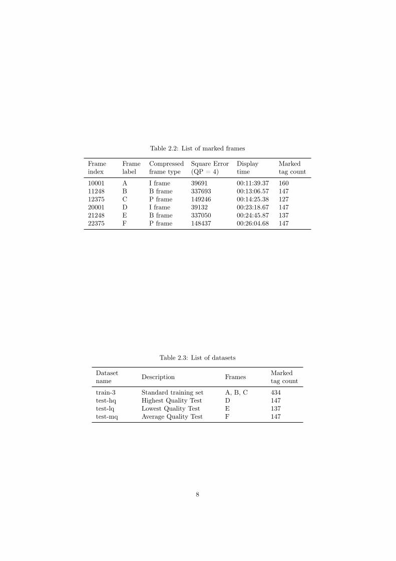
Table 2.2: List of marked frames
Frameindex
Framelabel
Compressedframe type
Square Error(QP = 4)
Displaytime
Markedtag count
10001 A I frame 39691 00:11:39.37 16011248 B B frame 337693 00:13:06.57 14712375 C P frame 149246 00:14:25.38 12720001 D I frame 39132 00:23:18.67 14721248 E B frame 337050 00:24:45.87 13722375 F P frame 148437 00:26:04.68 147
Table 2.3: List of datasets
Datasetname Description Frames Marked
tag count
train-3 Standard training set A, B, C 434test-hq Highest Quality Test D 147test-lq Lowest Quality Test E 137test-mq Average Quality Test F 147
8
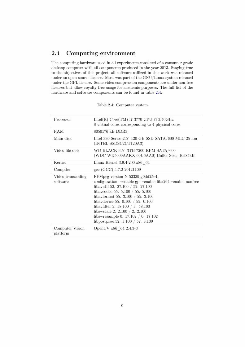
2.4 Computing environmentThe computing hardware used in all experiments consisted of a consumer gradedesktop computer with all components produced in the year 2013. Staying trueto the objectives of this project, all software utilized in this work was releasedunder an open-source license. Most was part of the GNU/Linux system releasedunder the GPL license. Some video compression components are under non-freelicenses but allow royalty free usage for academic purposes. The full list of thehardware and software components can be found in table 2.4.
Table 2.4: Computer system
Processor Intel(R) Core(TM) i7-3770 CPU @ 3.40GHz8 virtual cores corresponding to 4 physical cores
RAM 8050176 kB DDR3
Main disk Intel 330 Series 2.5” 120 GB SSD SATA/600 MLC 25 nm(INTEL SSDSC2CT120A3)
Video file disk WD BLACK 3.5” 3TB 7200 RPM SATA/600(WDC WD5000AAKX-60U6AA0) Buffer Size: 16384kB
Kernel Linux Kernel 3.9.4-200 x86_64
Compiler gcc (GCC) 4.7.2 20121109
Video transcoding FFMpeg version N-52339-g0dd25e4software configuration: –enable-gpl –enable-libx264 –enable-nonfree
libavutil 52. 27.100 / 52. 27.100libavcodec 55. 5.100 / 55. 5.100libavformat 55. 3.100 / 55. 3.100libavdevice 55. 0.100 / 55. 0.100libavfilter 3. 58.100 / 3. 58.100libswscale 2. 2.100 / 2. 2.100libswresample 0. 17.102 / 0. 17.102libpostproc 52. 3.100 / 52. 3.100
Computer Vision OpenCV x86_64 2.4.3-3platform
9
Chapter 3
Video Preprocessing
There are two types of characteristics of the video frames that are useful intracking the bees:
Tags: Obviously, the tags are the best source of information regarding themovement of the bees. The actual coordinate of a bee, the orientation ofits head and its unique ID can be determined just from decoding the tag.
Edges: Certain interactions between bees such as trophallaxis and touching ofantennae cannot be inferred from the tags. Bodily protrusions of beeshave clearly defined edges, which can be used in accurate measurement ofantennae and tongue activity.
Preprocessing applied to the video should emphasize or at least preservethese two types of image characteristics.
3.1 Video compressionThe sheer size of the video is a major limiting factor in the length of time beemovements can be recorded. For example, a movie file of around 11 hours and15 minutes takes up around 870 GiB of disk space, not accounting for the filesystem overhead. Apart from storage, the movie data stream requires a largebandwidth when read, which limits the speed the video can be processed afteracquisition, regardless of raw processing power [13].
3.1.1 CroppingThe original frame size is 1626× 1236 pixels. It differs slightly from the actualcapability of the camera (1628× 1236) in that the width of the former is not amultiple of 4. Video encoding software packages like Mencoder [14] discouragestoring video data with frame width that is not a multiple of 4 since it inter-feres with word alignment in many recent processors [13] and requires excessiveoverhead in many popular compression schemes. Aside from the width problem,upper and lower parts of the video frame consistently display the wooden frameused to contain the bees, which is of no use in tracking the bees. For full codeccompatibility, the frames were cropped to the lowest possible multiples of 16 in
10
both width and height in such a way as to not affect the area where bees canmove.
3.1.2 Huffman YUVThe software product used to record the original video, Virtual VCR [15] onlysupported Huffman YUV compression [10]. Interestingly, the developer speci-fication states that the frame width must be a multiple of 4 yet the softwaremanaged to bypass this limitation. The encoded format may not be supportedby other decoders or players that comply to the HuffmanYUV standard.
The HuffmanYUV format uses intra-frame compression in that frames areprocessed independently of each other. The pixels values of a frame are scannedin sequence. A pixel at a particular location in this sequence is predicted usinga simple heuristic, such as the median, applied to several of the preceding pixels.The difference between the actual and the predicted pixel value is compressedusing Huffman coding [16]. This method is lossless in that the original uncom-pressed video can be reconstructed without error from the compressed format.The somewhat misleading term YUV refers to the fact that the codec requiresthat image data be stored in YCrCb format. RGB color space values R, G andB can be converted to Y, Cb and Cr by the following relation [17], assuming allintensities are represented by values in the interval [0, 255]:
Y = 0.299 ·R+ 0.587 ·G+ 0.114 ·BCb = −0.1687 ·R− 0.3313 ·G+ 0.5 ·B + 128
Cr = 0.5 ·R− 0.4187 ·G− 0.0813 ·B + 128
(3.1)
The extra chroma channels do not increase the file size considerably sincethey are always zero and always predicted accurately by most heuristics.
Nevertheless, for the 11 hour video file d1_140812.avi mentioned previously,HuffmanYUV produces an average compressed frame size of around 1684 KiBout of an uncompressed size of 1965 KiB yielding an 85.7% compression ra-tio. The reduction in file size does not offset the compression/decompressionoverhead and the need for an index when seeking to a particular frame. Poten-tially lossy methods need to be employed in order to get the file size one order ofmagnitude lower to a level that makes recording of long video sequences feasible.
3.1.3 H.264/AVCAs of year 2013, the H.264 is the de facto format for high-quality video com-pression in the multimedia industry [12]. A reference implementation H.264encoder is part of the SPEC2006 benchmarks, which are an integral part ofthe design process of CPU architectures such as the Intel Core [13]. H.264 issometimes referred to as Advanced Video Coding (AVC) and H.264 and AVCcan be used interchangeably.
H.264 encoding reduces file size by discarding information that is not per-ceived by the human visual system. Lossless compression is also possible byexploiting both spatial (intra-frame) and temporal (inter-frame) statistical re-dundancies.
11
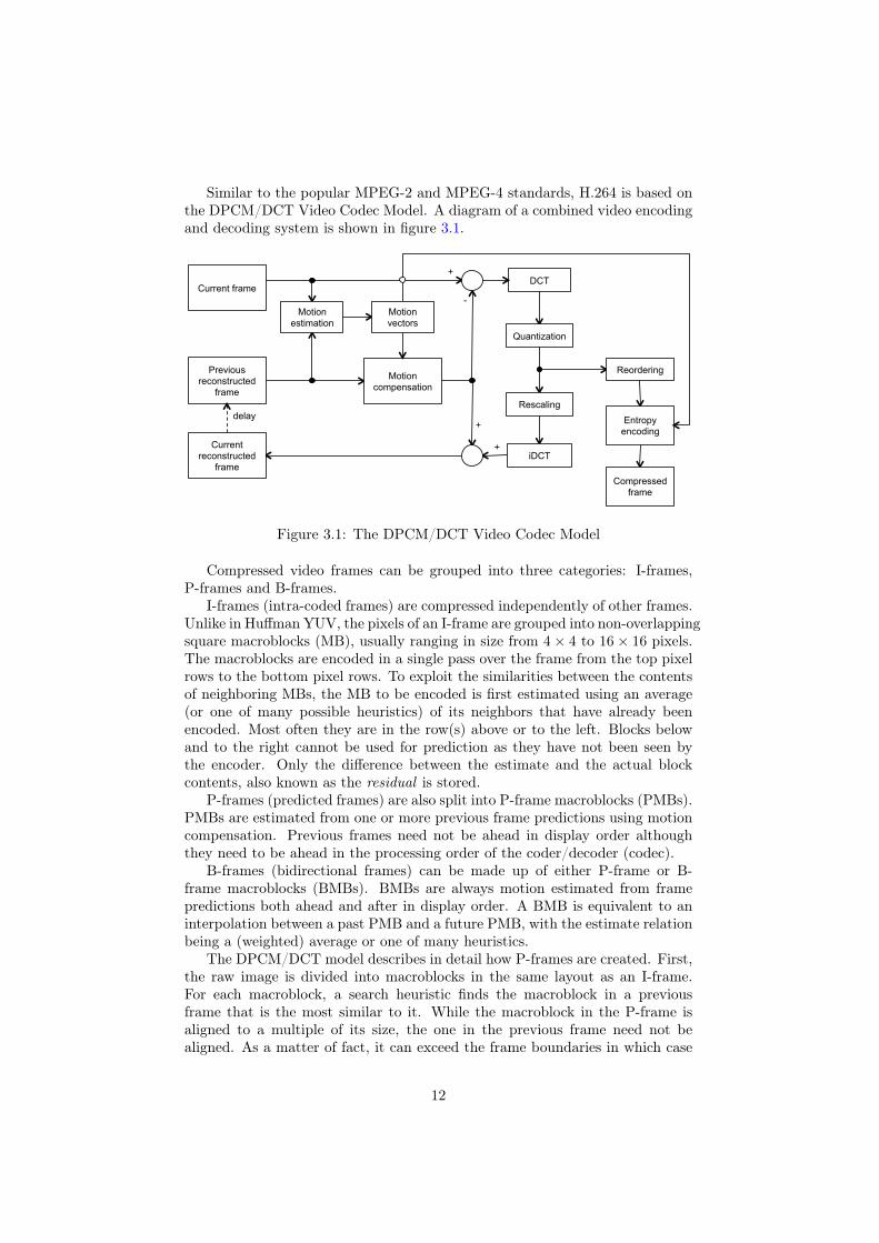
Similar to the popular MPEG-2 and MPEG-4 standards, H.264 is based onthe DPCM/DCT Video Codec Model. A diagram of a combined video encodingand decoding system is shown in figure 3.1.
Current frame
Previous reconstructed
frame
Motion estimation
DCT +
-
+
+
Motion compensation
Quantization
Current reconstructed
frame
Reordering
Entropy encoding
Compressed frame
delay Rescaling
iDCT
Motion vectors
Figure 3.1: The DPCM/DCT Video Codec Model
Compressed video frames can be grouped into three categories: I-frames,P-frames and B-frames.
I-frames (intra-coded frames) are compressed independently of other frames.Unlike in Huffman YUV, the pixels of an I-frame are grouped into non-overlappingsquare macroblocks (MB), usually ranging in size from 4× 4 to 16× 16 pixels.The macroblocks are encoded in a single pass over the frame from the top pixelrows to the bottom pixel rows. To exploit the similarities between the contentsof neighboring MBs, the MB to be encoded is first estimated using an average(or one of many possible heuristics) of its neighbors that have already beenencoded. Most often they are in the row(s) above or to the left. Blocks belowand to the right cannot be used for prediction as they have not been seen bythe encoder. Only the difference between the estimate and the actual blockcontents, also known as the residual is stored.
P-frames (predicted frames) are also split into P-frame macroblocks (PMBs).PMBs are estimated from one or more previous frame predictions using motioncompensation. Previous frames need not be ahead in display order althoughthey need to be ahead in the processing order of the coder/decoder (codec).
B-frames (bidirectional frames) can be made up of either P-frame or B-frame macroblocks (BMBs). BMBs are always motion estimated from framepredictions both ahead and after in display order. A BMB is equivalent to aninterpolation between a past PMB and a future PMB, with the estimate relationbeing a (weighted) average or one of many heuristics.
The DPCM/DCT model describes in detail how P-frames are created. First,the raw image is divided into macroblocks in the same layout as an I-frame.For each macroblock, a search heuristic finds the macroblock in a previousframe that is the most similar to it. While the macroblock in the P-frame isaligned to a multiple of its size, the one in the previous frame need not bealigned. As a matter of fact, it can exceed the frame boundaries in which case
12
the part outside the frame is usually padded with zeroes. The displacement,called a motion vector is stored. The collection of motion vectors is used togenerate a motion compensated version of the P-frame. The difference, alsocalled the residual, is transformed to the frequency domain using the DiscreteCosine Transform (DCT). Given a pixel intensity representation of the residualintensities E = (ex,y), x, y ∈ {0, ..., N − 1} where N is the macroblock size, thefrequency domain representation F = (fi,j) is expressed as F = A × E × ATwhere:
Ax,y = Cx · cos
((2 · y + 1) · x · π
2 ·N
)and Cx =
√
1N when x = 0√2N when x > 0
(3.2)
The corresponding inverse transform iDCT is given by E = AT × F × A.The H.264 standard requires that the integer transform be used. It is an ap-proximation of DCT with the added benefit that no information is lost throughrounding to nearest integers.
The only step when information loss can occur is quantization. When a scalarquantizer is used, the integer frequency values fx,y are divided by a scalar calledthe quantizer or quantization parameter QP yielding the quantized coefficientsqx,y:
qx,y = round
(fx,yQP
)(3.3)
If a QP of 0 is specified, the encoder will skip this step (qx,y = fx,y) andcreate a bit stream from which the original video can be recreated without error.
Next, the coefficients are scanned, most often on a diagonal starting from thetop-left corner, and turned into a data stream. The motion vectors computedin the motion estimation stage are difference coded and then concatenated tothis stream. The entire resulting sequence is compressed in a lossless fashionusing an entropy encoder. The size of the data is drastically reduced becausethe integer transform produces many small values, which are clamped to zero inthe quantization stage. Like in Huffman coding, the entropy encoder produceslonger symbols for less frequent values. However, it uses a predefined symboltable. Huffman coding needs to scan the data in order to compute the proba-bility of occurrence for each symbol before starting the actual encoding process.The entropy encoder can process the data in a single pass and output symbolson the fly. It also takes advantage of the fact that the data stream contains longsequences of zero values by explicitly encoding run lengths of zero.
The symbol list is then stored in the video file. H.264 specifies only theencoding of the video data. How video and audio data are related, the index ofthe video frames for seeking, and other information is stored in the container,which has its own specification. In order to decode the video file, both thecontainer and H.264 must be supported by the software system.
As mentioned previously, the motion estimation is based on the estimationof frames instead of original frames. This is to prevent the phenomenon calleddrift. If instead of the estimation, the raw frame would be used in the prediction,the errors in decompressing the residual would accumulate in time leading toan excessive loss of quality. Using the prediction instead keeps the error withinbounds. In order to make predictions based on estimations, the encoder mustalso employ a decoder during compression.
13
Once the video data and the container are produced, they can be stored orstreamed for later use.
The decoding process is the reverse of the encoding, where the opposite ofquantization is rescaling :
fx,y = qx,y ·QP (3.4)
where fx,y is the estimate of the original frequency coefficients fi,j . The residualpixel intensity estimates ei,j are obtained by iDCT from fi,j .
The motion compensation is then added to the residual to obtain the frameestimate ix,y.
The MSE quality measureKnowing that the decoded frames are merely an approximation of the originalones, a measure of quality needs to be defined. This area has been the focusof extensive research. Measures that attempt at defining the video quality asperceived by humans include Just Noticeable Difference (JDD), Digital VideoQuality (DVQ) and Structural Similarity Index (SSIM) to name a few [12].In this work, compression constitutes a necessary preprocessing step for im-age analysis methodologies introduced in later sections. Information normallydiscarded by the human visual system may still relevant and, as such, the sim-ple and mathematically rigorous Mean Square Error (MSE) may be a betterperformance predictor for automated methods than those intended for subjec-tive quality assessment. MSE is defined as the average pixel-by-pixel squaredifference between the original and predicted frames:
MSE =1
W ·H·
(W−1∑x=0
H−1∑y=0
(ix,y − ix,y)2
)(3.5)
where W and H are the frame width and height, respectively.
x264x264 [11] is a computationally efficient free and open-source H.264 encoding soft-ware package. It is employed in several web video services such as YouTube [18]and Vimeo [11]. The source code is optimized for the GCC compiler and IntelCore architecture, which makes it a good match for the computing environmentutilized in this project.
YUV 4:2:0x264 requires that the raw video frame be encoded in the YUV 4:2:0 format.Pixels are grouped in 2 × 2 pixel non-overlapping square regions. For eachregion, 4 luminance (Y) and one of each chroma values (Cr, Cb) are stored. Thisimposes the constraint that both the width and height of the frame be multiplesof two. The luminance and chroma are stored separately, due to their differentsampling frequencies. For the video files used in this project, the chroma valuesare both zero yet have to be explicitly specified when processed by x264. Theentropy coding ensures that the chroma components have a negligible impacton file size.
14
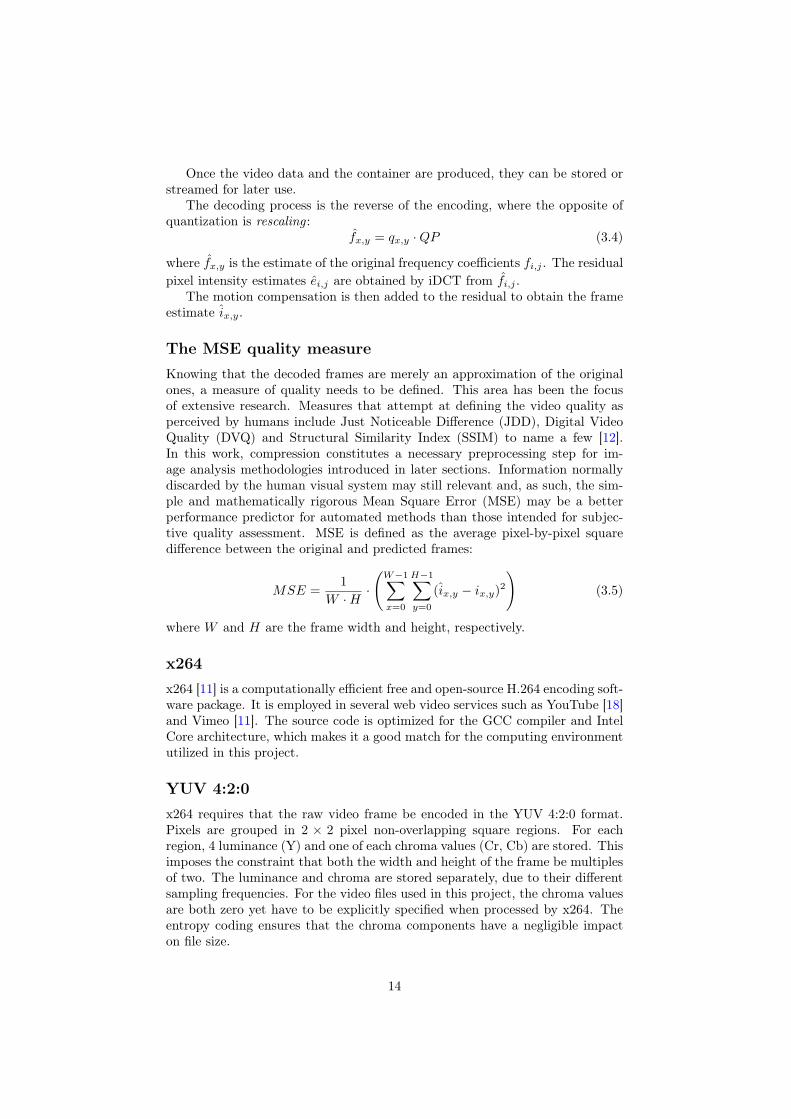
3.1.4 x264 performanceIn order to obtain an accurate estimate of the compression performance of x264,the entire 1 hour long video d1_140812.avi was compressed using fixed scalarquantizers ranging from 0 to 40 with an increment of 4. The YUV 4:2:0 colorspace used was yuv420p instead of the default yuvj420p. The default colorspace maps several gray levels to a single value, leading to information loss.
On the whole video
The source video was read and the compressed video was written at the sametime from the video file hard-disk unit. As it is evident from figure 3.2, de-spite the excessive disk usage, the encoding time was less than the durationof the source video (3600 sec) for all QP values tested. Therefore, faster thanreal-time encoding is possible. Lossless compression does not employ a quanti-zation step so it encodes video faster than with quantizer 4. For low quantizers,motion estimation behaves in the same way as in lossless coding and quanti-zation merely adds complexity to the encoding process while offering little filesize reduction. As the quantizer increases, the compression time drops almostexponentially. One reason is that higher quantizers map many DCT coefficientsto zero. Processing long runs of zero is faster and the entropy encoder pro-duces fewer symbols. Also, disk reads and writes limit the performance of theencoding, regardless of CPU processing power. The smaller the compressed bitstream, the less data is written to disk shifting the compression burden fromthe disk to the CPU.
500
1000
1500
2000
2500
3000
3500
0 4 8 12 16 20 24 28 32 36 40
Encoding time (sec)
Scalar quantizer (QP) value
x264 encoding time for a 3600 sec video
Figure 3.2: x264 encoding time of a 1 hour long video
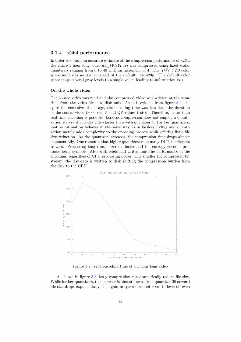
As shown in figure 3.3, lossy compression can dramatically reduce file size.While for low quantizers, the decrease is almost linear, from quantizer 20 onwardfile size drops exponentially. The gain in space does not seem to level off even
15
at the highest quantizer setting tested (QP = 40). At this point, the perceivedquality was too low to warrant going further.
102
103
104
105
0 4 8 12 16 20 24 28 32 36 40
Compressed file size (MiB)
Scalar quantizer (QP) value
x264 compressed file size
Figure 3.3: Compressed size of a 1 hour long video
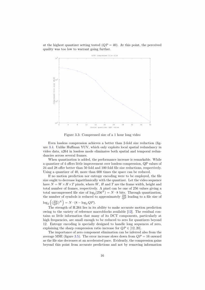
Even lossless compression achieves a better than 2-fold size reduction (fig-ure 3.4. Unlike Huffman YUV, which only exploits local spatial redundancy invideo data, x264 in lossless mode eliminates both spatial and temporal redun-dancies across several frames.
When quantization is added, the performance increase is remarkable. Whilea quantizer of 4 offers little improvement over lossless compression, QP values of24 and 28 offer better than 50 fold and 100 fold file size reductions, respectively.Using a quantizer of 40, more than 600 times the space can be reduced.
If no motion prediction nor entropy encoding were to be employed, the filesize ought to decrease logarithmically with the quantizer. Let the video sequencehave N = W×H×T pixels, whereW , H and T are the frame width, height andtotal number of frames, respectively. A pixel can be one of 256 values giving atotal uncompressed file size of log2(256N ) = N · 8 bits. Through quantization,the number of symbols is reduced to approximately 256
QP leading to a file size of
log2
(( 256QP )N
)= N · (8− log2QP ).
The strength of H.264 lies in its ability to make accurate motion predictionowing to the variety of reference macroblocks available [12]. The residual con-tains so little information that many of its DCT components, particularly athigh frequencies, are small enough to be reduced to zero for quantizers beyond12. Entropy encoding is specially designed to handle long sequences of zero,explaining the sharp compression ratio increase for QP ∈ [12, 20].
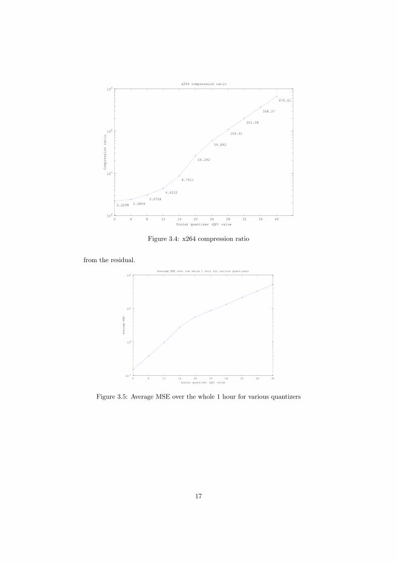
The importance of zero component elimination can be inferred also from theaverage MSE (figure 3.5). The error increase slows down from QP = 16 onwardas the file size decreases at an accelerated pace. Evidently, the compression gainsbeyond this point from accurate predictions and not by removing information
16
100
101
102
103
0 4 8 12 16 20 24 28 32 36 40
Compression ratio
Scalar quantizer (QP) value
x264 compression ratio
2.2298 2.3859
3.0728
4.4222
8.7911
26.292
59.892
109.91
201.08
368.37
670.61
Figure 3.4: x264 compression ratio
from the residual.
10-1
100
101
102
4 8 12 16 20 24 28 32 36 40
Average MSE
Scalar quantizer (QP) value
Average MSE over the whole 1 hour for various quantizers
Figure 3.5: Average MSE over the whole 1 hour for various quantizers
17
Frame by frame
In order to understand how quality varies across the frames for very long se-quences, frame by frame MSE values were computed for various quantizersacross the entire hour long video.
Lossless compression did perform as expected, with MSE = 0 for everyframe analyzed. In terms of frame mix, the 51481 frame sequence was encodedusing 206 I-frames, 51275 P-frames and no B-frames.
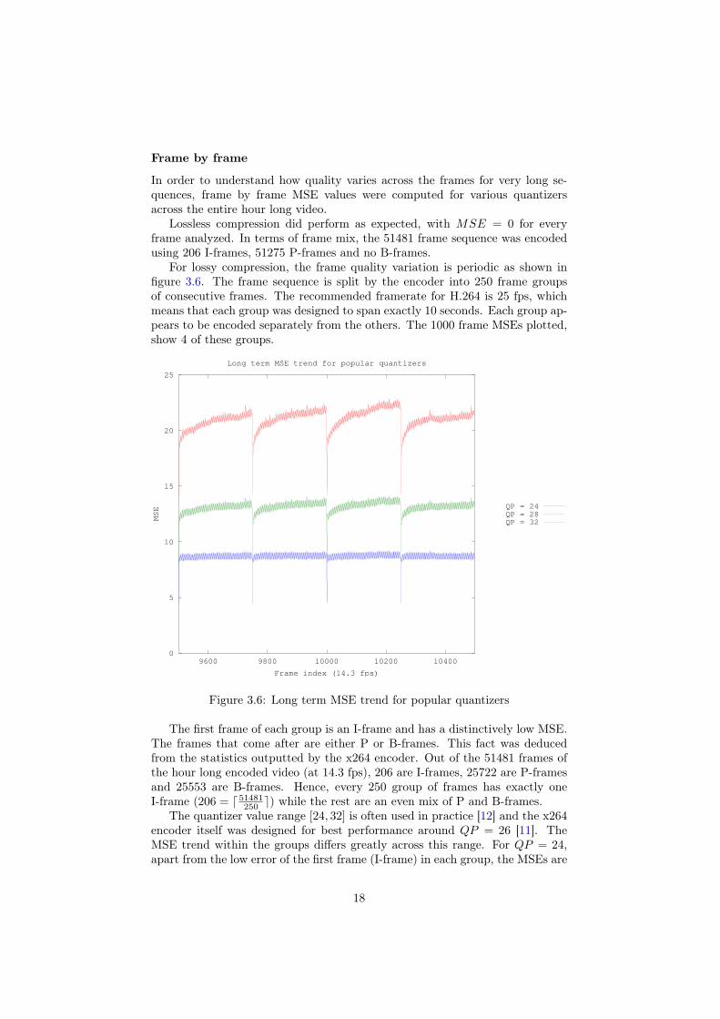
For lossy compression, the frame quality variation is periodic as shown infigure 3.6. The frame sequence is split by the encoder into 250 frame groupsof consecutive frames. The recommended framerate for H.264 is 25 fps, whichmeans that each group was designed to span exactly 10 seconds. Each group ap-pears to be encoded separately from the others. The 1000 frame MSEs plotted,show 4 of these groups.
0
5
10
15
20
25
9600 9800 10000 10200 10400
MSE
Frame index (14.3 fps)
Long term MSE trend for popular quantizers
QP = 24QP = 28QP = 32
Figure 3.6: Long term MSE trend for popular quantizers
The first frame of each group is an I-frame and has a distinctively low MSE.The frames that come after are either P or B-frames. This fact was deducedfrom the statistics outputted by the x264 encoder. Out of the 51481 frames ofthe hour long encoded video (at 14.3 fps), 206 are I-frames, 25722 are P-framesand 25553 are B-frames. Hence, every 250 group of frames has exactly oneI-frame (206 = d 51481
250 e) while the rest are an even mix of P and B-frames.The quantizer value range [24, 32] is often used in practice [12] and the x264
encoder itself was designed for best performance around QP = 26 [11]. TheMSE trend within the groups differs greatly across this range. For QP = 24,apart from the low error of the first frame (I-frame) in each group, the MSEs are
18
stable. Quantizing the difference between the current frame and the estimateof the previously encoded frames prevents error accumulation or drift for thesesettings. For QP = 32, this balance breaks down and quality steadily degradesas the frames are farther away from the first (I-frame) in the group. A new groupresets the MSE, which results in long term error stability. In this sense, the I-frames act as ”fire-walls”, preventing errors from accumulating beyond them.Moreover, if the bit stream contained errors, I-frames ensure that at most 250frames are affected. They are also useful in seeking at random points in video.To decompress any random frame, at most 250 frames need be read, startingwith the I-frame of that group.
In the case of the hour-long video, the 264 encoder selected different quan-tizer values for the three types of frames. Given a global quantization parameterQP , I-frames are compressed with QP − 3, P-frames with QP and B-frameswith QP + 2. I-frames have no motion prediction and thus larger residuals. Alower quantizer is required to encode them accurately enough. Furthermore,the quality of the entire frame group depends on this frame and, since it is veryinfrequent, more space can be used to encode it. B-frames on the other handrely on a great deal more motion compensation than any other frames meaningthat their smaller residuals can withstand more quality loss.
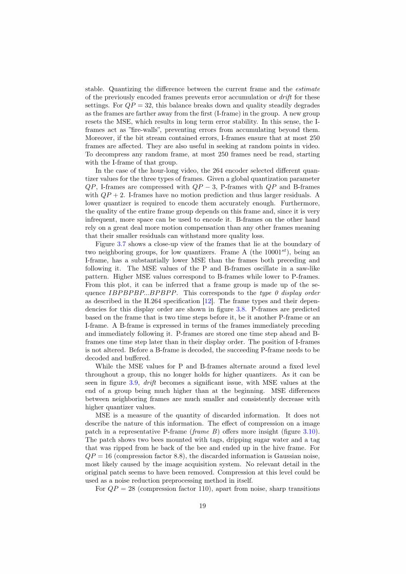
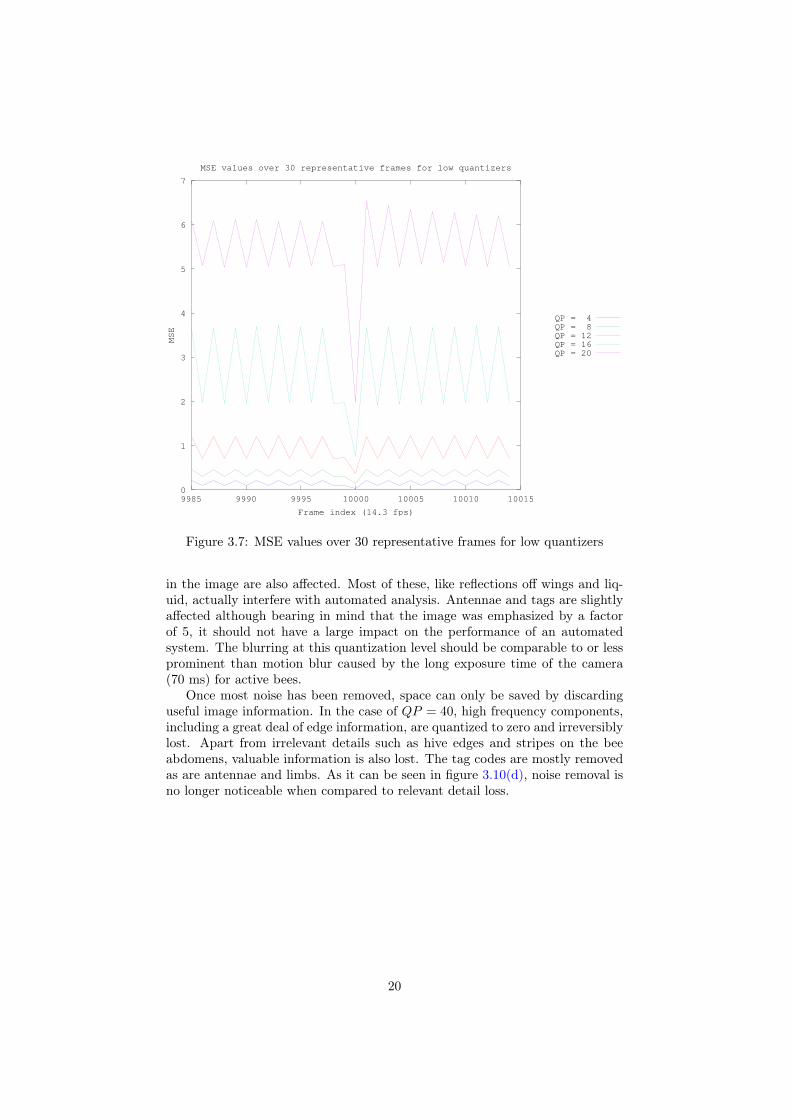
Figure 3.7 shows a close-up view of the frames that lie at the boundary oftwo neighboring groups, for low quantizers. Frame A (the 10001st), being anI-frame, has a substantially lower MSE than the frames both preceding andfollowing it. The MSE values of the P and B-frames oscillate in a saw-likepattern. Higher MSE values correspond to B-frames while lower to P-frames.From this plot, it can be inferred that a frame group is made up of the se-quence IBPBPBP...BPBPP . This corresponds to the type 0 display orderas described in the H.264 specification [12]. The frame types and their depen-dencies for this display order are shown in figure 3.8. P-frames are predictedbased on the frame that is two time steps before it, be it another P-frame or anI-frame. A B-frame is expressed in terms of the frames immediately precedingand immediately following it. P-frames are stored one time step ahead and B-frames one time step later than in their display order. The position of I-framesis not altered. Before a B-frame is decoded, the succeeding P-frame needs to bedecoded and buffered.
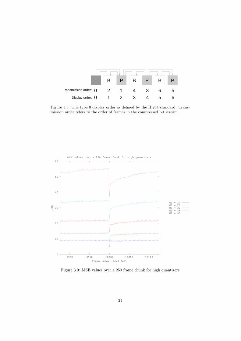
While the MSE values for P and B-frames alternate around a fixed levelthroughout a group, this no longer holds for higher quantizers. As it can beseen in figure 3.9, drift becomes a significant issue, with MSE values at theend of a group being much higher than at the beginning. MSE differencesbetween neighboring frames are much smaller and consistently decrease withhigher quantizer values.
MSE is a measure of the quantity of discarded information. It does notdescribe the nature of this information. The effect of compression on a imagepatch in a representative P-frame (frame B) offers more insight (figure 3.10).The patch shows two bees mounted with tags, dripping sugar water and a tagthat was ripped from he back of the bee and ended up in the hive frame. ForQP = 16 (compression factor 8.8), the discarded information is Gaussian noise,most likely caused by the image acquisition system. No relevant detail in theoriginal patch seems to have been removed. Compression at this level could beused as a noise reduction preprocessing method in itself.
For QP = 28 (compression factor 110), apart from noise, sharp transitions
19
0
1
2
3
4
5
6
7
9985 9990 9995 10000 10005 10010 10015
MSE
Frame index (14.3 fps)
MSE values over 30 representative frames for low quantizers
QP = 4QP = 8QP = 12QP = 16QP = 20
Figure 3.7: MSE values over 30 representative frames for low quantizers
in the image are also affected. Most of these, like reflections off wings and liq-uid, actually interfere with automated analysis. Antennae and tags are slightlyaffected although bearing in mind that the image was emphasized by a factorof 5, it should not have a large impact on the performance of an automatedsystem. The blurring at this quantization level should be comparable to or lessprominent than motion blur caused by the long exposure time of the camera(70 ms) for active bees.
Once most noise has been removed, space can only be saved by discardinguseful image information. In the case of QP = 40, high frequency components,including a great deal of edge information, are quantized to zero and irreversiblylost. Apart from irrelevant details such as hive edges and stripes on the beeabdomens, valuable information is also lost. The tag codes are mostly removedas are antennae and limbs. As it can be seen in figure 3.10(d), noise removal isno longer noticeable when compared to relevant detail loss.
20
I B P B P B P
0 2 1 4 3 6 5
0 1 2 3 4 5 6
Transmission order:
Display order:
Figure 3.8: The type 0 display order as defined by the H.264 standard. Trans-mission order refers to the order of frames in the compressed bit stream.
0
10
20
30
40
50
60
9900 9950 10000 10050 10100
MSE
Frame index (14.3 fps)
MSE values over a 250 frame chunk for high quantizers
QP = 24QP = 28QP = 32QP = 36QP = 40
Figure 3.9: MSE values over a 250 frame chunk for high quantizers
21
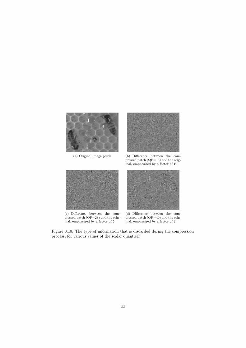
(a) Original image patch (b) Difference between the com-pressed patch (QP=16) and the orig-inal, emphasized by a factor of 10
(c) Difference between the com-pressed patch (QP=28) and the orig-inal, emphasized by a factor of 5
(d) Difference between the com-pressed patch (QP=40) and the orig-inal, emphasized by a factor of 2
Figure 3.10: The type of information that is discarded during the compressionprocess, for various values of the scalar quantizer
22
3.2 Background removalThe scenes are stationary with respect to the hive frame and the field of viewhas been cropped to encompass precisely the region where bees are allowed tomove. Apart from the moving bees, the video images contain hexagonal hivecells and a small part of the wooden outer frame as background. The hive frameand outer frame remain mostly unaltered throughout the video sequence. In thefuture, bees may be filmed long enough to lay eggs and seal hive cells to keepsustenance and larvae. For the time being, however, the background is of leastconcern to this project.
At first, whether the background hinders the segmentation of the bees wasstudied.
Edge imageAn edge image was obtained using an established method: the Canny edgedetector [19]. This method was designed to identify true edges in the presenceof noise, based on low pass filtering and connected components. First, thepixels in the original image ix,y are smoothed using a Gaussian filter of standarddeviation σ yielding the image fx,y. The kernel of the Gaussian filter is givenby:
Gx,y =1√
2 · π · σ· e−
x2+y2
2·σ2 (3.6)
The σ parameter controls minimum distance between two different edges. Thegradients along the axes are computed as gx = ∂f
∂x and gy = ∂f∂y . Gradients can
be computed by convolving with either [-1 0 1] or [-1 1] kernels and their trans-positions. Next, the gradient magnitude Mx,y and direction αx,y are computedusing:
Mx,y =√g2x + g2
y (3.7)
αx,y =
{arctan
gygx
if gx 6= 0
sign(gy) · π2 if gx = 0(3.8)
Magnitude tends to be high in non-edge pixels so nonmaxima suppression isused. For every pixel, the gradient direction αx,y is rounded to the closestmultiple of π
4 , giving one of the 8 directions dk. If the magnitude of a pixel isnot greater than the magnitude of either neighboring pixels along dk, it is set tozero. Intuitively, edges should be one pixel thick and nonmaxima suppressionis a way of thinning the edges.
Two binary images lx,y and hx,y are obtained by thresholding the magnitudeat every pixel with a low threshold TL and a high threshold TH , respectively.The final edge image is the collection of pixels obtained by 8-neighborhoodflood-filling lx,y with seeds in hx,y. Edge pixels in lx,y that are not reached bythe flood-filling are removed. This is called hysteresis thresholding.
The utilized implementation, part of the OpenCV library [20], was designedfor low computational cost and it differs from the original Canny method. Gaus-sian smoothing and gradient calculations were approximated with two Sobel fil-ters [21]. The L2 norm in edge magnitude was approximated with the L1 normas it does not require computing the square root.
23
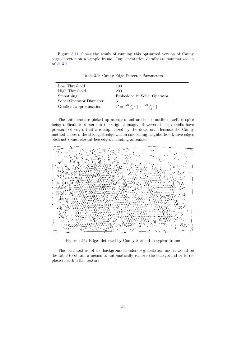
Figure 3.11 shows the result of running this optimized version of Cannyedge detector on a sample frame. Implementation details are summarized intable 3.1.
Table 3.1: Canny Edge Detector Parameters
Low Threshold 100High Threshold 200Smoothing Embedded in Sobel OperatorSobel Operator Diameter 3Gradient approximation G = |dI(x,y)
dx |+ |dI(x,y)dy |
The antennae are picked up as edges and are hence outlined well, despitebeing difficult to discern in the original image. However, the hive cells havepronounced edges that are emphasized by the detector. Because the Cannymethod chooses the strongest edge within smoothing neighborhood, hive edgesobstruct some relevant bee edges including antennae.
Figure 3.11: Edges detected by Canny Method in typical frame
The local texture of the background hinders segmentation and it would bedesirable to obtain a means to automatically remove the background or to re-place it with a flat texture.
24
3.2.1 ClusteringSegmentation can be performed by classifying local texture as belonging to eitherbackground or foreground. The large variety of textures makes manual texturelabeling tedious. If a large corpus of texture prototypes were to be generatedautomatically, dividing the corpus into bee and background sections would bea less daunting task.
In unsupervised learning, a system learns how to represent data based on aquality measure that is defined independently of the task at hand [22]. Apartfrom the measure, no manual input is necessary making it a viable preprocessingprocedure for large sets of data.
Clustering is a form of unsupervised learning where data points are assignedgroupings based on a similarity measure. One of the most simple and robustunsupervised clustering methods is K-means clustering [23]. It uses squaredEuclidean distance as the similarity measure and the sum of intra-class variancesas a data representation quality measure.
Texture based segmentation requires that a mathematical model of texturebe specified. For simplicity, local texture is defined in this work as a pixel-wisetransform of a square patch centered at a particular location (x, y) as ~tx,y =f (ix+x′,y+y′) where x′, y′ ∈ {−r, ..., r} , r is the (Manhattan distance circle)radius of that patch and f is the transform, often a normalization function.
The textures can be scanned from top-down and then left-right making themone-dimensional vectors ~tx,y = (vj) where j ∈ {0, ...,m − 1} is an integer. Thelength of the vector is given by m = (2 · r + 1)2. The textures themselves canbe serialized as to not depend to their center coordinates and are indexed as ti,where i ∈ {0, ..., n− 1} (not to be confused with ix,y) and n is the total numberof texture samples gathered. An individual texture value can be expressed asvi,j where i is the texture index and j is the location within the texture.
Clusters are defined as the partition of the set {0, ..., n−1} into mutually dis-joint subsets Ck that minimizes the objective function J(C). The total numberof clusters K is decided beforehand. The objective function is given by:
J(C) =1
2·K∑k=1
∑i,i′∈Ck
d(~ti,~ti′) (3.9)
where d is the square of the Euclidean distance:
d(~ti,~ti′) =∑
j,j′∈{0,...,m−1}
(vi,j − vi′,j′)2 (3.10)
The advantage of K-means is in that the objective function reduces to:
J(C) =
K∑k=1
∑i∈Ck
d(~ti − µk
)(3.11)
where µk is the centroid of Ck, the average of all textures assigned to Ck.Unlike other learning systems, K-means is transparent in that µk is a texturethat defines its cluster (a prototype).
The calculation of the prototypes is accomplished through an iterative de-scent algorithm:
25
1. Start with a number of clusters K and a value for each µk computed basedon some heuristic on the data.
2. For each k, compute Ck as the set of indices i such that ~ti is closer to µkthan any other µk′ , k 6= k′.
3. Update for cluster µk to be the average of all ~ti, i ∈ Ck.
4. If no µk has changed in this iteration or a certain number of iterations hasbeen reached, terminate the algorithm. Otherwise go back to step 2.
Since the number of clusters is to be specified a priori and greatly affects theoutcome, a large number of clusters was chosen. The initial cluster positionswere chosen as random patches from a video frame. As the illumination and thestructure of the frames changes little throughout the sequence, it is assumedthat it is very likely that patches from one frame can be also found in otherframes. The high number of patches also means that the centroids span thetexture space evenly with high probability.
Shadows may induce unwanted variance and can be alleviated by normaliza-tion. The simplest way is to bring all pixel values of the neighborhood into thesame fixed range. This can be accomplished through min-max normalization.The pixel values can be linearly mapped to span the interval [0, 255]. Letminx,yand maxx,y be the minimum and maximum values of the image patch centeredat (x, y):
minx,y = minx′,y′∈{−r,...,r}
ix+x′,y+y′ (3.12)
maxx,y = maxx′,y′∈{−r,...,r}
ix+x′,y+y′ (3.13)
The normalization function f is:
f(ix,y) = 255 · ix,y −minx,ymaxx,y −minx,y
(3.14)
Another normalization method is Gaussian normalization. Let µx,y and σx,ybe the mean and standard deviation of the image patch centered at (x, y):
µx,y =1
(2 · r + 1)2·
∑x′,y′∈{−r,...,r}
ix+x′,y+y′ (3.15)
σx,y =
√∑x′,y′∈{−r,...,r}(ix+x′,y+y′ − µx,y)2
(2 · r + 1)2 − 1(3.16)
giving a normalization function
f(ix,y) = saturate(
128 + 128 · ix,y − µx,yσx,y
)(3.17)
where the values are saturated to the interval [0, 255] by:
saturate(x) =
0 if x < 0
x if 0 ≤ x ≤ 255
255 if x > 255
(3.18)
26
Gaussian normalization is robust even in the presence of shot noise in theimaging system or glares caused by dripping liquid. Nonetheless, it cannotguarantee that no pixel values get perturbed by saturation nor that the [0, 255]range can be covered efficiently.
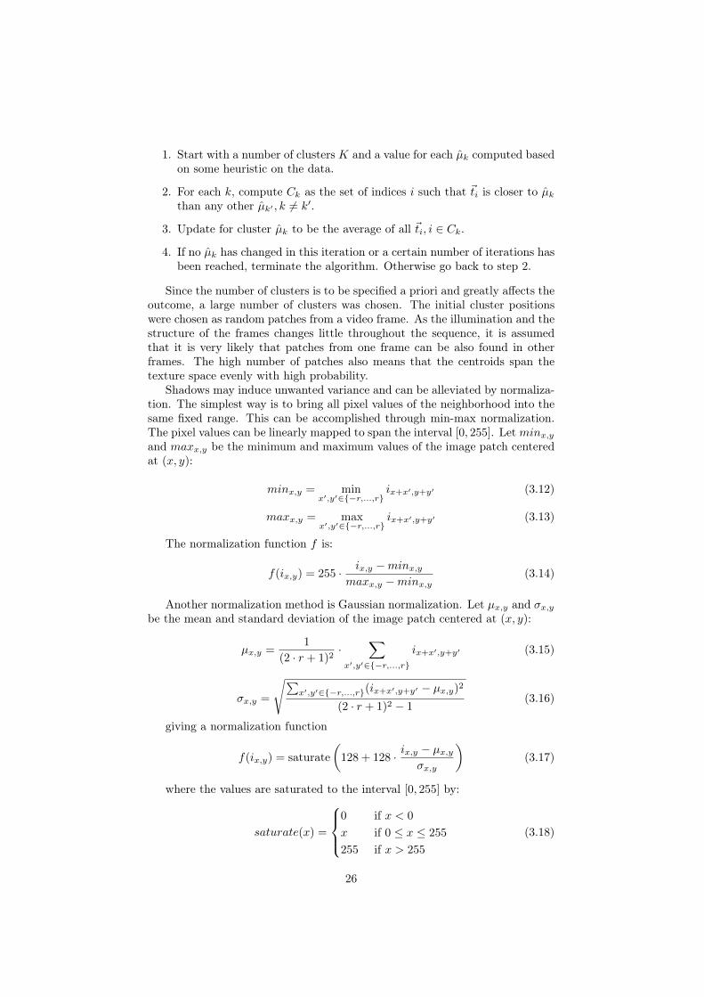
The centroid (prototype) textures for 64 clusters obtained through each nor-malization technique are shown in figure 3.12.
(a) No normalization. Texturessorted by average value
(b) Gaussian Normalization
(c) Min-max Normalization
Figure 3.12: Results of running K-means clustering on a typical frame (frameA) using 11 x 11 pixel patches and 64 clusters
Because the hive cells are regular, the space of all possible cell textures issmall. Also, most of the video frame is made up of cells and the initial clusterseeding was made with equal probability over the image. Most clusters arecreated to represent cells. The combined effect is that the cell texture prototypesconverge to strong, regular, well defined features. Bees are highly irregular andregions of the video frame containing bees have fewer cluster assigned to them.The clusters that describe bee regions end up covering heterogeneous regions intexture space and thus the prototypes are averaged away into smooth gradients.
In particular for small neighborhoods, deciding which clusters belong to beesand which to background can be challenging. Larger neighborhoods require alarge number of clusters to be created in order to span a high dimensional texturespace. In this case, manually selecting which clusters belong to bees and whichto background is tedious. To facilitate the selection, regions in frame A were
27
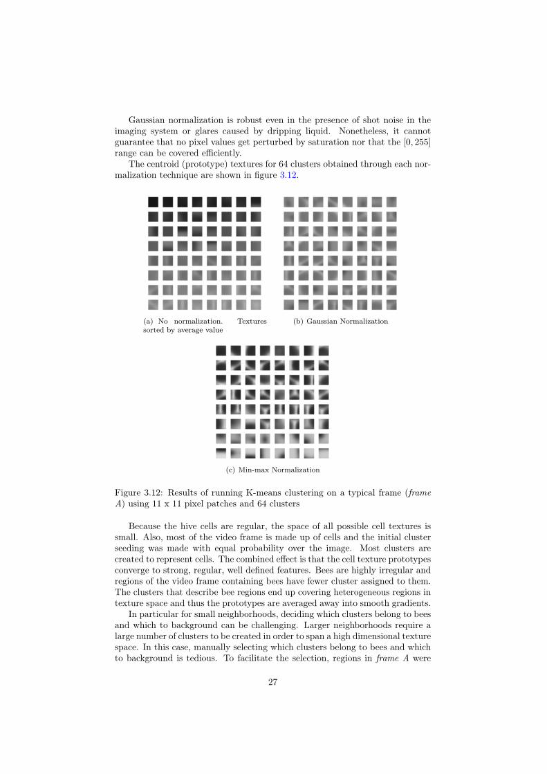
manually marked with red for definitely background and green for definitelybee. Areas of the image were left unpainted as it was difficult to establish whichpixels belonged to bees and which to background in the vicinity of bee bodiesand under shadows. This human editable image was transformed into a singlechannel image as in figure 3.13. The gray valued pixels are considered unlabeledand not used in training or testing.
Figure 3.13: Training data for supervised post-processing
Next, the nearest cluster for each pixel in the frame image was computed.As a result, each cluster has been assigned a collection of pixels. By replacingthe pixels with their corresponding labels, each cluster thus has a positive labelcount and negative label count. Ideally, each cluster should have one of thesecounts equal to zero. In practice, each cluster has a pixel classification error, ormisclassification impurity.
Since the number of positive labels differs from the negative labels, the countsneed to be normalized using:
Pf = count(foreground)prior_count(foreground)
Pb = count(background)prior_count(background)
(3.19)
to account for the prior imbalance and
pf =Pf
Pf+Pb
pb = PbPf+Pb
(3.20)
to make sure that the probabilities sum up to 1.There are several measures of impurity, the most common being:
• Misclassification Impurity: Mi = 1−max(pf , pb)
• Gini impurity: Gi = 2 · pf · pb
28
• Entropy impurity: Ei = −pf · log2(pf )− pb · log2(pb)
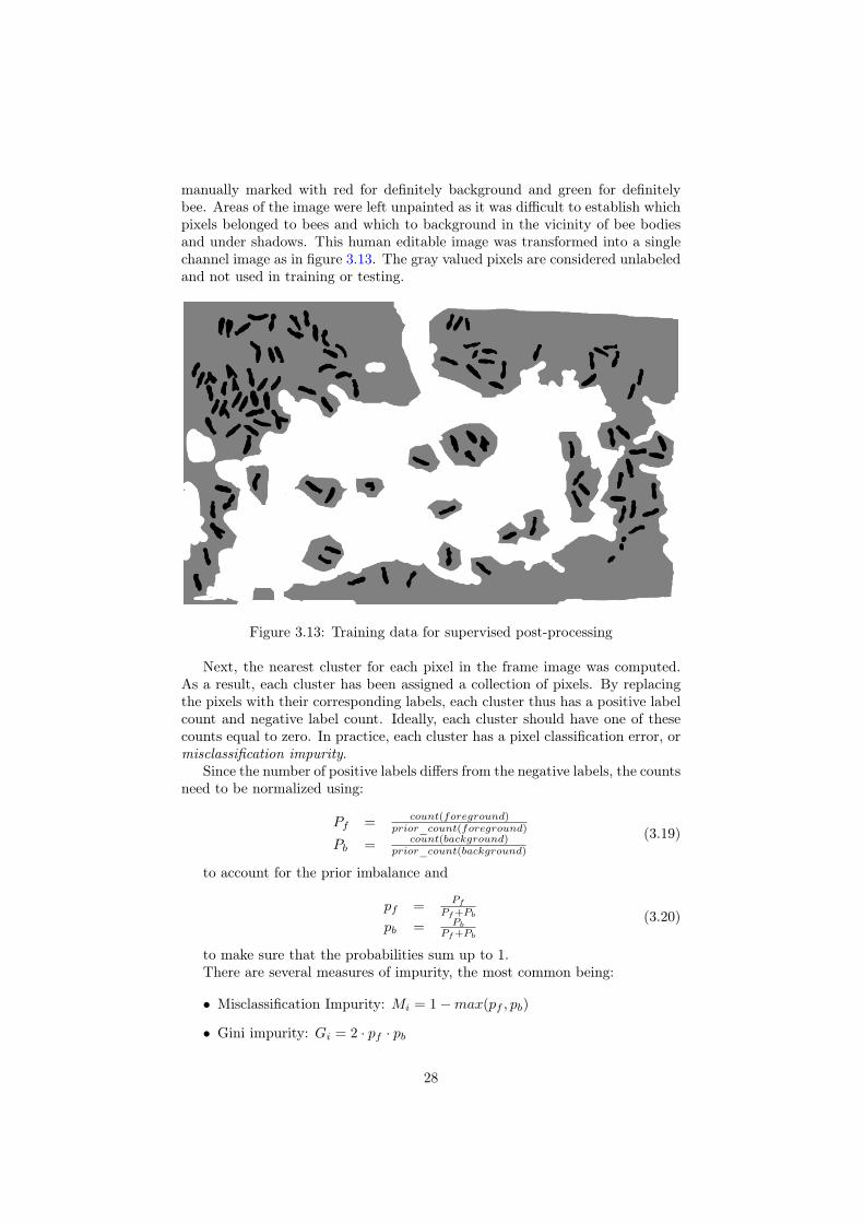
Min-max normalization gave the lowest overall impurity values and theseare shown in figure 3.14. The clusters were sorted by the normalized positiveprobability. Regardless of the measure used, cluster impurity remains withinthe 20% - 80% range.
0
0.2
0.4
0.6
0.8
1
1.2
10 20 30 40 50 60
Classification impurity of the clusters on the training data
Positive ProbabilityImpurity
GiniEntropy
Figure 3.14: Classification purity on training image
The clusters are assigned labels, either positive, or negative based on whichnormalized probability is greater. The label assignment is discrete, not fuzzy,and the purity measure is not taken into account. Because each pixel in theimage can have the closest cluster assigned to it and the clusters are classifiedthemselves into two classes, a binary classification of the pixels themselves ispossible. Figure 3.15 shows the classification of the training image itself.
Hive cell edges are correctly classified as background. Most parts of bees arealso classified correctly despite the fact that only a few of them were markedin the training process. The hive cell centers, having a more even texture areincorrectly marked as belonging to bees. If the background regions were to beremoved and in-painted using the surrounding colors, edge detectors should notpick up hive cells while still focusing on antennae.
Normalized convolution was chosen as the inpainting procedure for its sim-plicity and speed of execution. This procedure takes two parameters: the orig-inal image ix,y and a mask bx,y that specifies which pixels are to be inpainted.
First, an inverse mask, fx,y = 255 − bx,y, is computed to designate whichpixels are to be left unchanged. The original image is masked with fx,y to yieldan image where all pixels to be estimated are set to black: fmx,y. This imageis blurred using a Gaussian filter yielding fgx,y. The σ parameter should belarge enough for the filter to fill in all the black pixels. Then the mask fx,y isblurred with the same Gaussian filter to give mgx,y. The ratio between fgx,yand mgx,y is used to fill in the original image at the pixels designated by the
29
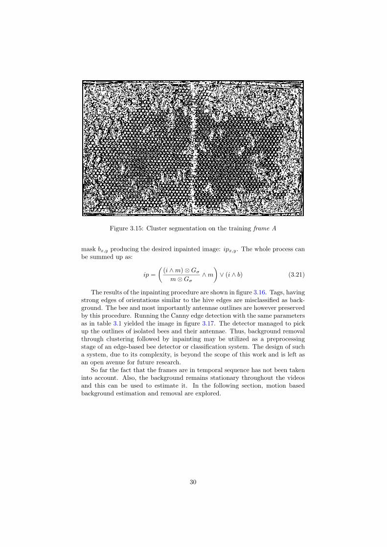
Figure 3.15: Cluster segmentation on the training frame A
mask bx,y producing the desired inpainted image: ipx,y. The whole process canbe summed up as:
ip =
((i ∧m)⊗Gσm⊗Gσ
∧m)∨ (i ∧ b) (3.21)
The results of the inpainting procedure are shown in figure 3.16. Tags, havingstrong edges of orientations similar to the hive edges are misclassified as back-ground. The bee and most importantly antennae outlines are however preservedby this procedure. Running the Canny edge detection with the same parametersas in table 3.1 yielded the image in figure 3.17. The detector managed to pickup the outlines of isolated bees and their antennae. Thus, background removalthrough clustering followed by inpainting may be utilized as a preprocessingstage of an edge-based bee detector or classification system. The design of sucha system, due to its complexity, is beyond the scope of this work and is left asan open avenue for future research.
So far the fact that the frames are in temporal sequence has not been takeninto account. Also, the background remains stationary throughout the videosand this can be used to estimate it. In the following section, motion basedbackground estimation and removal are explored.
30
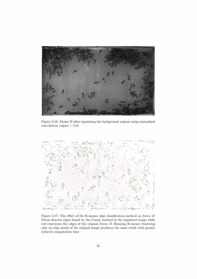
Figure 3.16: Frame D after inpainting the background regions using normalizedconvolution (sigma = 2.0)
Figure 3.17: The effect of the K-means edge classification method on frame D.Green denotes edges found by the Canny method in the inpainted image whilered represents the edges of the original frame D. Running K-means clusteringonly on edge pixels of the original image produces the same result with greatlyreduced computation time
31
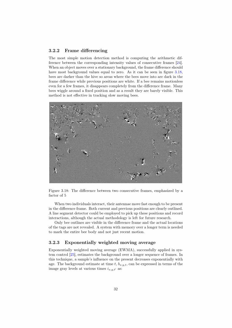
3.2.2 Frame differencingThe most simple motion detection method is computing the arithmetic dif-ference between the corresponding intensity values of consecutive frames [24].When an object moves over a stationary background, the frame difference shouldhave most background values equal to zero. As it can be seen in figure 3.18,bees are darker than the hive so areas where the bees move into are dark in theframe difference while previous positions are white. If a bee remains motionlesseven for a few frames, it disappears completely from the difference frame. Manybees wiggle around a fixed position and as a result they are barely visible. Thismethod is not effective in tracking slow moving bees.
Figure 3.18: The difference between two consecutive frames, emphasized by afactor of 5
When two individuals interact, their antennae move fast enough to be presentin the difference frame. Both current and previous positions are clearly outlined.A line segment detector could be employed to pick up these positions and recordinteractions, although the actual methodology is left for future research.
Only bee outlines are visible in the difference frame and the actual locationsof the tags are not revealed. A system with memory over a longer term is neededto mark the entire bee body and not just recent motion.
3.2.3 Exponentially weighted moving averageExponentially weighted moving average (EWMA), successfully applied in sys-tem control [25], estimates the background over a longer sequence of frames. Inthis technique, a sample’s influence on the present decreases exponentially withage. The background estimate at time t, bx,y,t, can be expressed in terms of theimage gray levels at various times ix,y,t′ as:
32
bx,y,t =
∞∑t′=0
(βt′· ix,y,t−t′)
∞∑t′=0
βt′
(3.22)
where 0 < β < 1 is a parameter that controls how fast the weights decay.The total sum of the weights has to be 1 in order to prevent the backgroundestimate either vanishing to zero or growing out of control. By noting that thedenominator is equal to 1
1−β , the equation can be simplified with the substitutionβ = 1− α:
bx,y,t = α · (∞∑t′=0
(1− α)t′· ix,y,t−t′) (3.23)
where α is the learning rate, a parameter that controls how far in the past frameshave a non-negligible influence on the estimate. Equation 3.23 is equivalent tothe following recursive relation:
bx,y,t = α · ix,y,t + (1− α) · bx,y,t−1 (3.24)
The estimate can be updated in-place using only the current frame data,making EWMA very light in terms of both memory usage and computationalload. A minor drawback is that the background estimate has to be kept infloating point representation.
The background estimate and its removal are highly dependent on the valueof the learning rate and the background initialization. In this work, the estimateis at the beginning set to be the first frame processed, which does include thebees (foreground) as well. The result of EWMA background removal on frameA (the 10001st) for a large learning rate of α = 0.01 is shown in figure 3.19. Thebackground estimate has a been accumulated over 10000 frames. The weight ofthe initial background value is α · (1−α)10000 = 2.25 ·10−46, which is negligible.The initialization does not affect the estimate this far away in time althoughrecent frames do have a large weight. As a consequence, trails can be seen wherebees were recently moving as there is a delay until recent foreground values areeliminated from the background estimate.
Smaller learning rates result in a more equal weighting of past samples anda more robust background estimate. A drawback is that the background needsto accumulate over a very large number of frames in order to downplay the roleof the initialization. Figure 3.20 shows frame A with the background removedafter background accumulation over 10000 frames. The weights are spread outmore evenly. The previous frame has a weight of α · (1−α)1 = 0.99 · 10−4 whilethe first frame analyzed has a weight of α · (1 − α)10000 = 0.37 · 10−4. As theinitial estimate and following frames are difficult to eliminate, the initial beepositions linger as white blobs in the background removed frame.
33
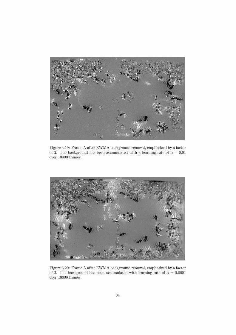
Figure 3.19: Frame A after EWMA background removal, emphasized by a factorof 2. The background has been accumulated with a learning rate of α = 0.01over 10000 frames.
Figure 3.20: Frame A after EWMA background removal, emphasized by a factorof 2. The background has been accumulated with learning rate of α = 0.0001over 10000 frames.
34
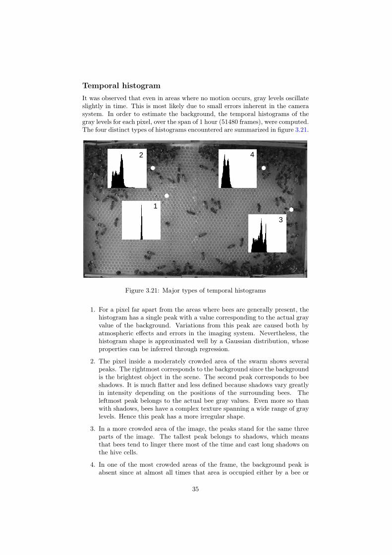
Temporal histogramIt was observed that even in areas where no motion occurs, gray levels oscillateslightly in time. This is most likely due to small errors inherent in the camerasystem. In order to estimate the background, the temporal histograms of thegray levels for each pixel, over the span of 1 hour (51480 frames), were computed.The four distinct types of histograms encountered are summarized in figure 3.21.
1
2
3
4
Figure 3.21: Major types of temporal histograms
1. For a pixel far apart from the areas where bees are generally present, thehistogram has a single peak with a value corresponding to the actual grayvalue of the background. Variations from this peak are caused both byatmospheric effects and errors in the imaging system. Nevertheless, thehistogram shape is approximated well by a Gaussian distribution, whoseproperties can be inferred through regression.
2. The pixel inside a moderately crowded area of the swarm shows severalpeaks. The rightmost corresponds to the background since the backgroundis the brightest object in the scene. The second peak corresponds to beeshadows. It is much flatter and less defined because shadows vary greatlyin intensity depending on the positions of the surrounding bees. Theleftmost peak belongs to the actual bee gray values. Even more so thanwith shadows, bees have a complex texture spanning a wide range of graylevels. Hence this peak has a more irregular shape.
3. In a more crowded area of the image, the peaks stand for the same threeparts of the image. The tallest peak belongs to shadows, which meansthat bees tend to linger there most of the time and cast long shadows onthe hive cells.
4. In one of the most crowded areas of the frame, the background peak isabsent since at almost all times that area is occupied either by a bee or
35

its shadow. Estimating the background from the temporal histogram isthe most difficult in this area.
In order to simplify the analysis of the background, several assumptions aremade in the beginning. These assumptions will be relaxed later on to yieldincreasingly complex models of the background. At first, it is assumed that:
1. The background can be considered an image, which does not change duringthe span of time the histograms were computed.
2. All histograms can be approximated by a single Gaussian distribution.
3. The proportion of non-background gray levels in every temporal histogramis negligible.
4. The background value is given by the mean of the Gaussian distribution.Even when the mean corresponds to a bee gray level, contrast can beincreased in this area to a level that can compensate for the backgroundremoval.
5. The variance of each individual Gaussian distribution is irrelevant sinceonly the mean is used.
6. The mean of every Gaussian distribution is given by a simple functioncomputed over the temporal gray-level histogram.
3.2.4 True averageFirst, it is assumed that the mean of the Gaussian distribution is approximatedwell by the average of the gray values over the entire time span the histogramswere computed. Given these assumptions, the estimate of the background image(bx,y) can be computed directly from the temporal histograms (hx,y(i)) as:
bx,y =
255∑i=0
(hx,y(i) · i)
255∑i=0
hx,y(i)
(3.25)
Here, all frames have equal influence on the background estimate. If the fore-ground pixels are evenly distributed both above and below background values,the average will successfully eliminate them.
3.2.5 Histogram peakAssuming that the mean of the Gaussian distribution corresponds to the highesthistogram count, the background image estimate is given by:
bx,y = arg maxi∈{0,...,255}
(hx,y(i)) (3.26)
A comparison between a patch in the average estimate and this peak estimateis shown in fig. 3.22. The peaks are susceptible to noise in the data, which
36
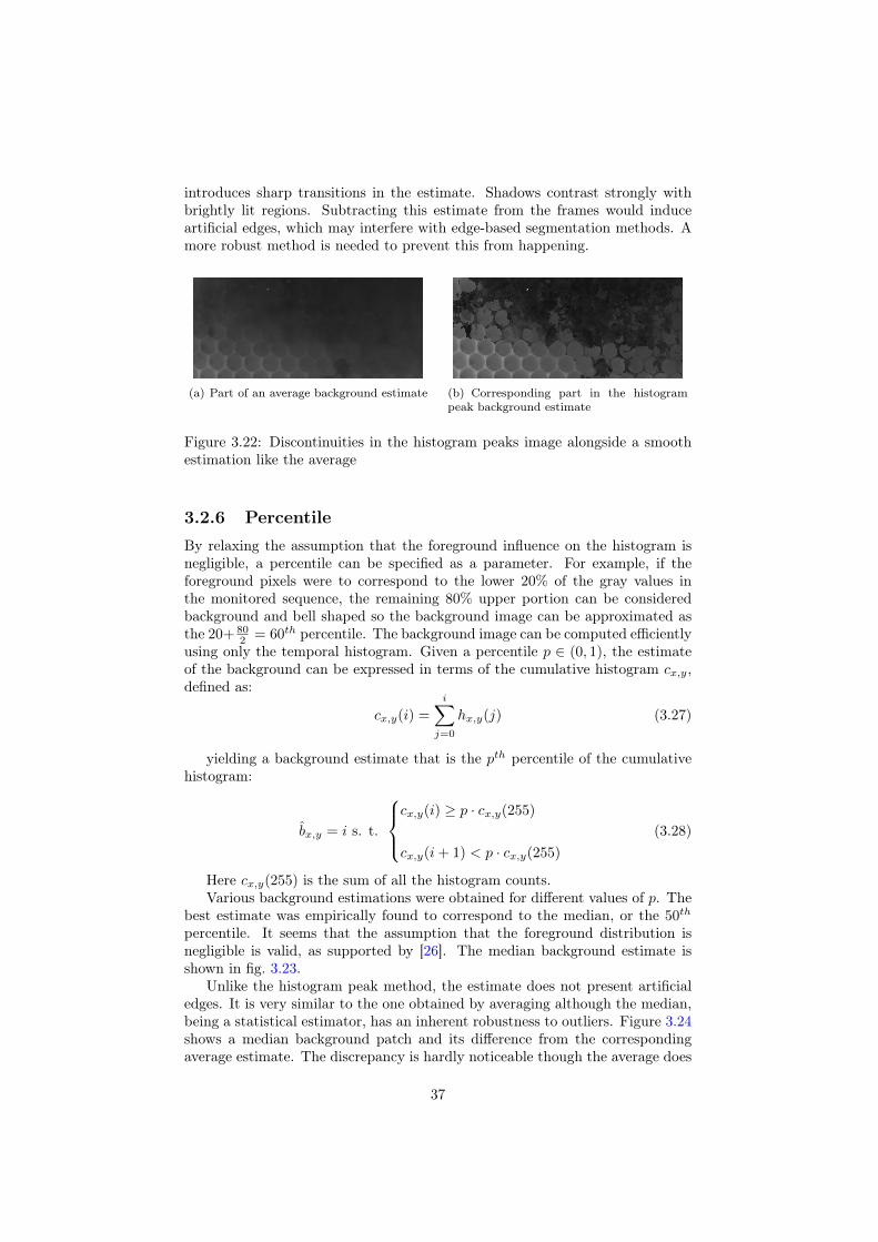
introduces sharp transitions in the estimate. Shadows contrast strongly withbrightly lit regions. Subtracting this estimate from the frames would induceartificial edges, which may interfere with edge-based segmentation methods. Amore robust method is needed to prevent this from happening.
(a) Part of an average background estimate (b) Corresponding part in the histogrampeak background estimate
Figure 3.22: Discontinuities in the histogram peaks image alongside a smoothestimation like the average
3.2.6 PercentileBy relaxing the assumption that the foreground influence on the histogram isnegligible, a percentile can be specified as a parameter. For example, if theforeground pixels were to correspond to the lower 20% of the gray values inthe monitored sequence, the remaining 80% upper portion can be consideredbackground and bell shaped so the background image can be approximated asthe 20+ 80
2 = 60th percentile. The background image can be computed efficientlyusing only the temporal histogram. Given a percentile p ∈ (0, 1), the estimateof the background can be expressed in terms of the cumulative histogram cx,y,defined as:
cx,y(i) =
i∑j=0
hx,y(j) (3.27)
yielding a background estimate that is the pth percentile of the cumulativehistogram:
bx,y = i s. t.
cx,y(i) ≥ p · cx,y(255)
cx,y(i+ 1) < p · cx,y(255)
(3.28)
Here cx,y(255) is the sum of all the histogram counts.Various background estimations were obtained for different values of p. The
best estimate was empirically found to correspond to the median, or the 50th
percentile. It seems that the assumption that the foreground distribution isnegligible is valid, as supported by [26]. The median background estimate isshown in fig. 3.23.
Unlike the histogram peak method, the estimate does not present artificialedges. It is very similar to the one obtained by averaging although the median,being a statistical estimator, has an inherent robustness to outliers. Figure 3.24shows a median background patch and its difference from the correspondingaverage estimate. The discrepancy is hardly noticeable though the average does
37
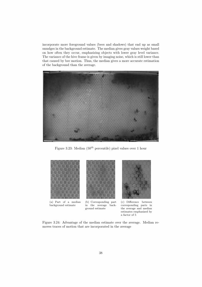
incorporate more foreground values (bees and shadows) that end up as smallsmudges in the background estimate. The median gives gray values weight basedon how often they occur, emphasizing objects with lower gray level variance.The variance of the hive frame is given by imaging noise, which is still lower thanthat caused by bee motion. Thus, the median gives a more accurate estimationof the background than the average.
Figure 3.23: Median (50th percentile) pixel values over 1 hour
(a) Part of a medianbackground estimate
(b) Corresponding partin the average back-ground estimate
(c) Difference betweencorresponding parts inthe average and medianestimates emphasized bya factor of 5
Figure 3.24: Advantage of the median estimate over the average. Median re-moves traces of motion that are incorporated in the average
38
3.2.7 Mixture of GaussiansRegular variations in the background such as shadows, can be accounted for byrelaxing the constraint that histograms take the form of a single Gaussian distri-bution. As stated in temporal histogram analysis, the temporal histogram canbe considered to be made up of 3 Gaussian distributions: regular background,shadows and bees.
This approximation can be computed online (at the same time as the framesare acquired) using the mixture of Gaussians (MOG) method [27]. In general,for every pixel in the frame a list of K Gaussian distributions is maintained.Each distribution k ∈ {0, ...,K − 1} has two parameters: the mean µk,t and thevariance σk,t. In addition, two more values are maintained: a weight wk,t anda background confidence value equal to wk,t
σk,t.
Given this model, the probability that the current gray level is observed isgiven by:
P (ix,y,t) =
K∑k=1
(wk,t · η(ix,y,t, µk,t, σk,t)) (3.29)
where η(ix,y,t, µk,t, σk,t) is the Gaussian probability density function of the kthGaussian distribution and is given by:
η(ix,y,t, µk,t, σk,t) =1√
2 · π · σk,t· exp
(− (ix,y,t − µk,t)2
2 · σ2k,t
)(3.30)
If the gray levels are observed over the 1 hour sequence, then, the probabilitydensity function P is actually given by the normalized histogram:
P (ix,y) =hx,y(ix,y)
255∑i′=0
hx,y(i′)
(3.31)
The weights wk,t express how frequent values belonging to the kth distri-bution are found at that position in the frame. Background gray values occurfrequently (high weight) and do not span a wide range (low variance). Whethera Gaussian distribution corresponds to background or not can be estimated bychecking whether that distribution has a high confidence value wk,t
σk,t.
Maintaining the temporal histogram and obtaining the Gaussian mixtureparameters by regression at every time step is too memory consuming and com-putationally intensive a task to be performed online. Instead a simple search isperformed. At every time step, the distributions are sorted by confidence valueso that the ones that are most likely to be background occur first. Then, fork increasing from 0, it is checked whether the new gray value ix,y,t falls within2.5 · σk,t−1. If a match is found, the search stops. Often, the distance betweenthe means of two Gaussian distributions is less than 5 · σk,t−1, meaning thatthey overlap. The MOG method gives precedence to background distributions.
If no match is found, the distribution most likely to be foreground is replacedwith a distribution centered at this gray value with a high variance and lowweight. Otherwise, the parameters of the matching distribution k are updated:
• The weight is brought closer to a value of 1:
39
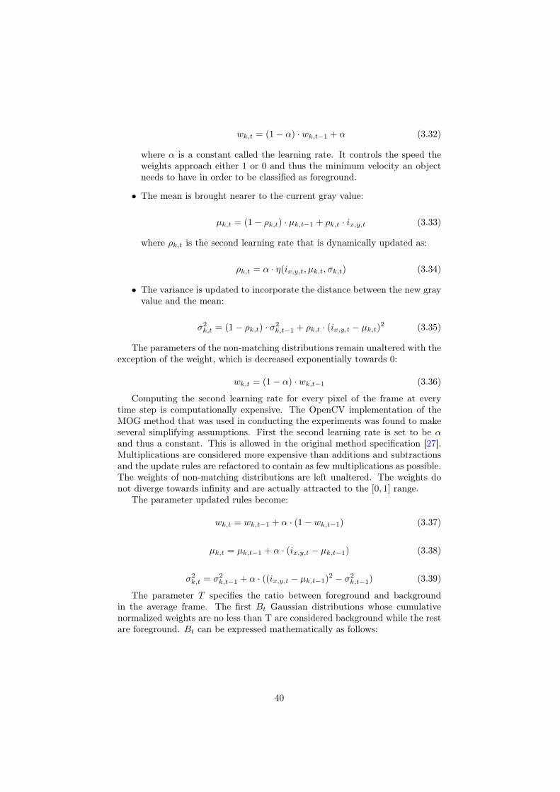
wk,t = (1− α) · wk,t−1 + α (3.32)
where α is a constant called the learning rate. It controls the speed theweights approach either 1 or 0 and thus the minimum velocity an objectneeds to have in order to be classified as foreground.
• The mean is brought nearer to the current gray value:
µk,t = (1− ρk,t) · µk,t−1 + ρk,t · ix,y,t (3.33)
where ρk,t is the second learning rate that is dynamically updated as:
ρk,t = α · η(ix,y,t, µk,t, σk,t) (3.34)
• The variance is updated to incorporate the distance between the new grayvalue and the mean:
σ2k,t = (1− ρk,t) · σ2
k,t−1 + ρk,t · (ix,y,t − µk,t)2 (3.35)
The parameters of the non-matching distributions remain unaltered with theexception of the weight, which is decreased exponentially towards 0:
wk,t = (1− α) · wk,t−1 (3.36)
Computing the second learning rate for every pixel of the frame at everytime step is computationally expensive. The OpenCV implementation of theMOG method that was used in conducting the experiments was found to makeseveral simplifying assumptions. First the second learning rate is set to be αand thus a constant. This is allowed in the original method specification [27].Multiplications are considered more expensive than additions and subtractionsand the update rules are refactored to contain as few multiplications as possible.The weights of non-matching distributions are left unaltered. The weights donot diverge towards infinity and are actually attracted to the [0, 1] range.
The parameter updated rules become:
wk,t = wk,t−1 + α · (1− wk,t−1) (3.37)
µk,t = µk,t−1 + α · (ix,y,t − µk,t−1) (3.38)
σ2k,t = σ2
k,t−1 + α · ((ix,y,t − µk,t−1)2 − σ2k,t−1) (3.39)
The parameter T specifies the ratio between foreground and backgroundin the average frame. The first Bt Gaussian distributions whose cumulativenormalized weights are no less than T are considered background while the restare foreground. Bt can be expressed mathematically as follows:
40
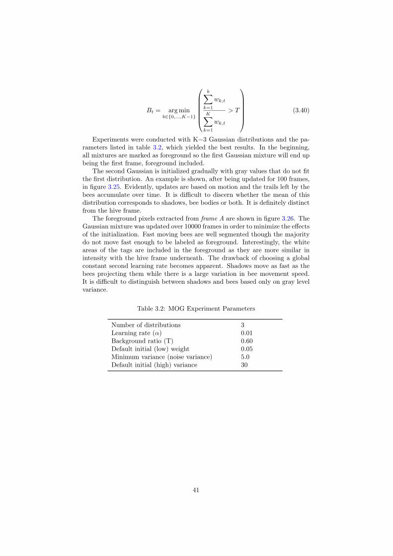
Bt = arg minb∈{0,...,K−1}
b∑
k=1
wk,t
K∑k=1
wk,t
> T
(3.40)
Experiments were conducted with K=3 Gaussian distributions and the pa-rameters listed in table 3.2, which yielded the best results. In the beginning,all mixtures are marked as foreground so the first Gaussian mixture will end upbeing the first frame, foreground included.
The second Gaussian is initialized gradually with gray values that do not fitthe first distribution. An example is shown, after being updated for 100 frames,in figure 3.25. Evidently, updates are based on motion and the trails left by thebees accumulate over time. It is difficult to discern whether the mean of thisdistribution corresponds to shadows, bee bodies or both. It is definitely distinctfrom the hive frame.
The foreground pixels extracted from frame A are shown in figure 3.26. TheGaussian mixture was updated over 10000 frames in order to minimize the effectsof the initialization. Fast moving bees are well segmented though the majoritydo not move fast enough to be labeled as foreground. Interestingly, the whiteareas of the tags are included in the foreground as they are more similar inintensity with the hive frame underneath. The drawback of choosing a globalconstant second learning rate becomes apparent. Shadows move as fast as thebees projecting them while there is a large variation in bee movement speed.It is difficult to distinguish between shadows and bees based only on gray levelvariance.
Table 3.2: MOG Experiment Parameters
Number of distributions 3Learning rate (α) 0.01Background ratio (T) 0.60Default initial (low) weight 0.05Minimum variance (noise variance) 5.0Default initial (high) variance 30
41
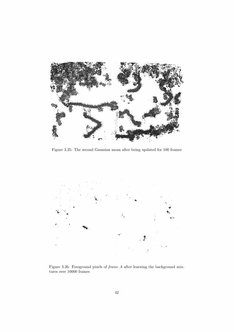
Figure 3.25: The second Gaussian mean after being updated for 100 frames
Figure 3.26: Foreground pixels of frame A after learning the background mix-tures over 10000 frames
42
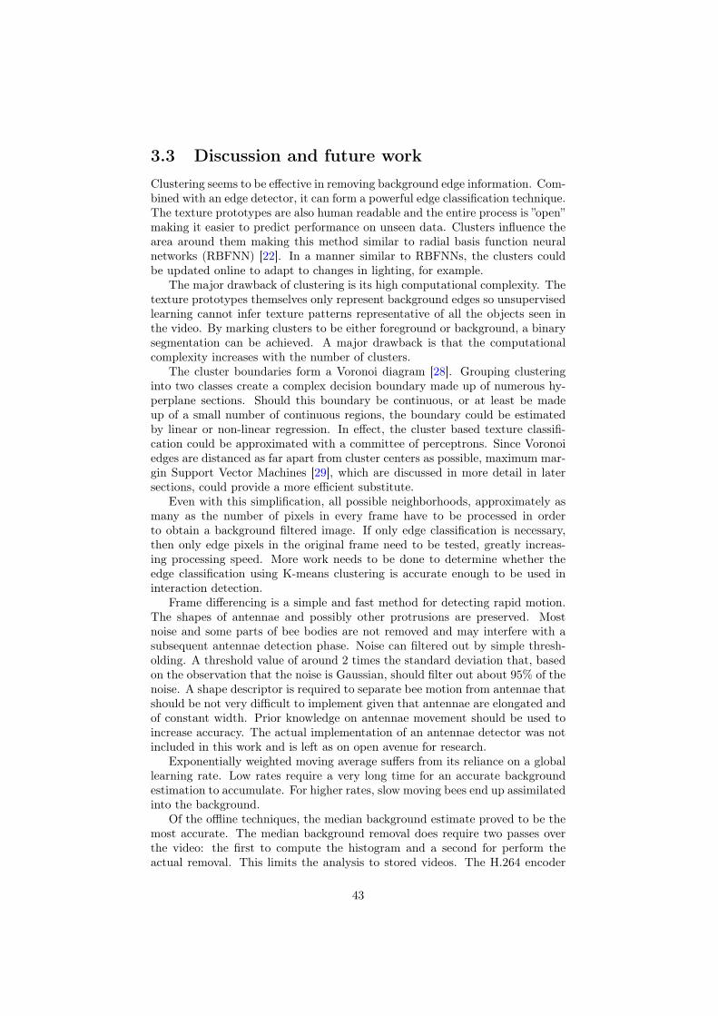
3.3 Discussion and future workClustering seems to be effective in removing background edge information. Com-bined with an edge detector, it can form a powerful edge classification technique.The texture prototypes are also human readable and the entire process is ”open”making it easier to predict performance on unseen data. Clusters influence thearea around them making this method similar to radial basis function neuralnetworks (RBFNN) [22]. In a manner similar to RBFNNs, the clusters couldbe updated online to adapt to changes in lighting, for example.
The major drawback of clustering is its high computational complexity. Thetexture prototypes themselves only represent background edges so unsupervisedlearning cannot infer texture patterns representative of all the objects seen inthe video. By marking clusters to be either foreground or background, a binarysegmentation can be achieved. A major drawback is that the computationalcomplexity increases with the number of clusters.
The cluster boundaries form a Voronoi diagram [28]. Grouping clusteringinto two classes create a complex decision boundary made up of numerous hy-perplane sections. Should this boundary be continuous, or at least be madeup of a small number of continuous regions, the boundary could be estimatedby linear or non-linear regression. In effect, the cluster based texture classifi-cation could be approximated with a committee of perceptrons. Since Voronoiedges are distanced as far apart from cluster centers as possible, maximum mar-gin Support Vector Machines [29], which are discussed in more detail in latersections, could provide a more efficient substitute.
Even with this simplification, all possible neighborhoods, approximately asmany as the number of pixels in every frame have to be processed in orderto obtain a background filtered image. If only edge classification is necessary,then only edge pixels in the original frame need to be tested, greatly increas-ing processing speed. More work needs to be done to determine whether theedge classification using K-means clustering is accurate enough to be used ininteraction detection.
Frame differencing is a simple and fast method for detecting rapid motion.The shapes of antennae and possibly other protrusions are preserved. Mostnoise and some parts of bee bodies are not removed and may interfere with asubsequent antennae detection phase. Noise can filtered out by simple thresh-olding. A threshold value of around 2 times the standard deviation that, basedon the observation that the noise is Gaussian, should filter out about 95% of thenoise. A shape descriptor is required to separate bee motion from antennae thatshould be not very difficult to implement given that antennae are elongated andof constant width. Prior knowledge on antennae movement should be used toincrease accuracy. The actual implementation of an antennae detector was notincluded in this work and is left as on open avenue for research.
Exponentially weighted moving average suffers from its reliance on a globallearning rate. Low rates require a very long time for an accurate backgroundestimation to accumulate. For higher rates, slow moving bees end up assimilatedinto the background.
Of the offline techniques, the median background estimate proved to be themost accurate. The median background removal does require two passes overthe video: the first to compute the histogram and a second for perform theactual removal. This limits the analysis to stored videos. The H.264 encoder
43
manages to reduce the file size by an order of magnitude while preserving therelevant details making offline methods practical. The one drawback, which isdifficult to alleviate is the effect of long term changes in the background suchas bees dying in the middle of the video.
The results of the mixture of Gaussians method were disappointing. Theapproximations made to speed up processing had a detrimental effect on fore-ground estimation. The MOG method was designed primarily to deal withrepeated variations in background. The bee shadow motions are closely linkedto bee motion and shadows and bee bodies appear to have overlapping graylevels. Offline sum of 3 Gaussians regression of the temporal histogram mayprove more effective though it should take into account that some distributionslike background or bees are absent from certain parts of the video.
In areas of the frame where the hive cells are almost always in shadow, it maybe more accurate to define the shadow itself as background and subtract it fromthe image. The median estimator seems to be the most suitable backgroundremoval method and it was chosen as the preprocessing step in the followingsection, which focuses on tag detection.
44
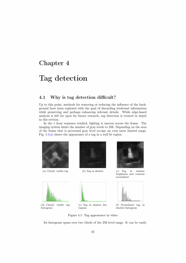
Chapter 4
Tag detection
4.1 Why is tag detection difficult?Up to this point, methods for removing or reducing the influence of the back-ground have been explored with the goal of discarding irrelevant informationwhile preserving and perhaps enhancing relevant details. While edge-basedanalysis is left for open for future research, tag detection is treated in depthin this section.
In the 1 hour sequence studied, lighting is uneven across the frame. Theimaging system limits the number of gray levels to 256. Depending on the areaof the frame that is processed gray level occupy an even more limited range.Fig. 4.1(a) shows the appearance of a tag in a well lit region.
(a) Clearly visible tag (b) Tag in shadow (c) Tag in shadowbrightness and contrastnormalized
0
2
4
6
8
10
12
14
0 50 100 150 200 250
(d) Clearly visible taghistogram
0
5
10
15
20
25
30
35
40
0 50 100 150 200 250
(e) Tag in shadow his-togram
0
5
10
15
20
25
30
35
40
-50 0 50 100 150 200 250 300
(f) Normalized tag inshadow histogram
Figure 4.1: Tag appearance in video
Its histogram spans over two thirds of the 256 level range. It can be easily
45
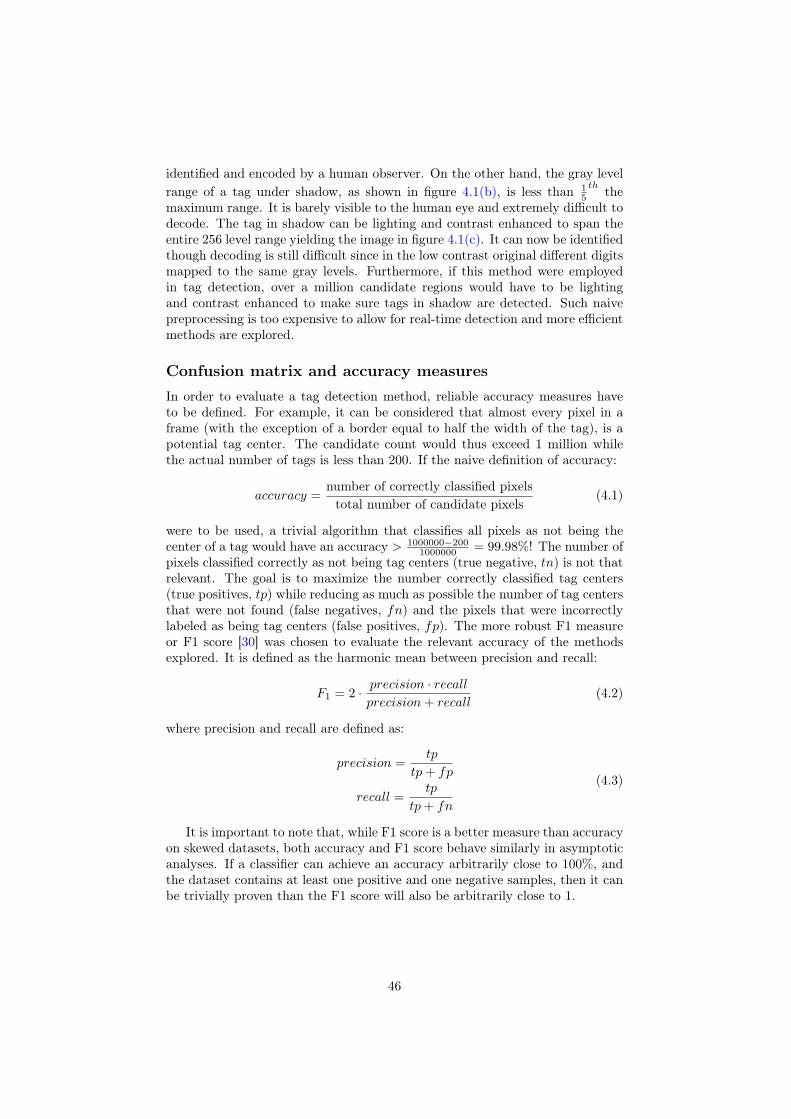
identified and encoded by a human observer. On the other hand, the gray levelrange of a tag under shadow, as shown in figure 4.1(b), is less than 1
5
th themaximum range. It is barely visible to the human eye and extremely difficult todecode. The tag in shadow can be lighting and contrast enhanced to span theentire 256 level range yielding the image in figure 4.1(c). It can now be identifiedthough decoding is still difficult since in the low contrast original different digitsmapped to the same gray levels. Furthermore, if this method were employedin tag detection, over a million candidate regions would have to be lightingand contrast enhanced to make sure tags in shadow are detected. Such naivepreprocessing is too expensive to allow for real-time detection and more efficientmethods are explored.
Confusion matrix and accuracy measuresIn order to evaluate a tag detection method, reliable accuracy measures haveto be defined. For example, it can be considered that almost every pixel in aframe (with the exception of a border equal to half the width of the tag), is apotential tag center. The candidate count would thus exceed 1 million whilethe actual number of tags is less than 200. If the naive definition of accuracy:
accuracy =number of correctly classified pixelstotal number of candidate pixels
(4.1)
were to be used, a trivial algorithm that classifies all pixels as not being thecenter of a tag would have an accuracy > 1000000−200
1000000 = 99.98%! The number ofpixels classified correctly as not being tag centers (true negative, tn) is not thatrelevant. The goal is to maximize the number correctly classified tag centers(true positives, tp) while reducing as much as possible the number of tag centersthat were not found (false negatives, fn) and the pixels that were incorrectlylabeled as being tag centers (false positives, fp). The more robust F1 measureor F1 score [30] was chosen to evaluate the relevant accuracy of the methodsexplored. It is defined as the harmonic mean between precision and recall:
F1 = 2 · precision · recallprecision+ recall
(4.2)
where precision and recall are defined as:
precision =tp
tp+ fp
recall =tp
tp+ fn
(4.3)
It is important to note that, while F1 score is a better measure than accuracyon skewed datasets, both accuracy and F1 score behave similarly in asymptoticanalyses. If a classifier can achieve an accuracy arbitrarily close to 100%, andthe dataset contains at least one positive and one negative samples, then it canbe trivially proven than the F1 score will also be arbitrarily close to 1.
46
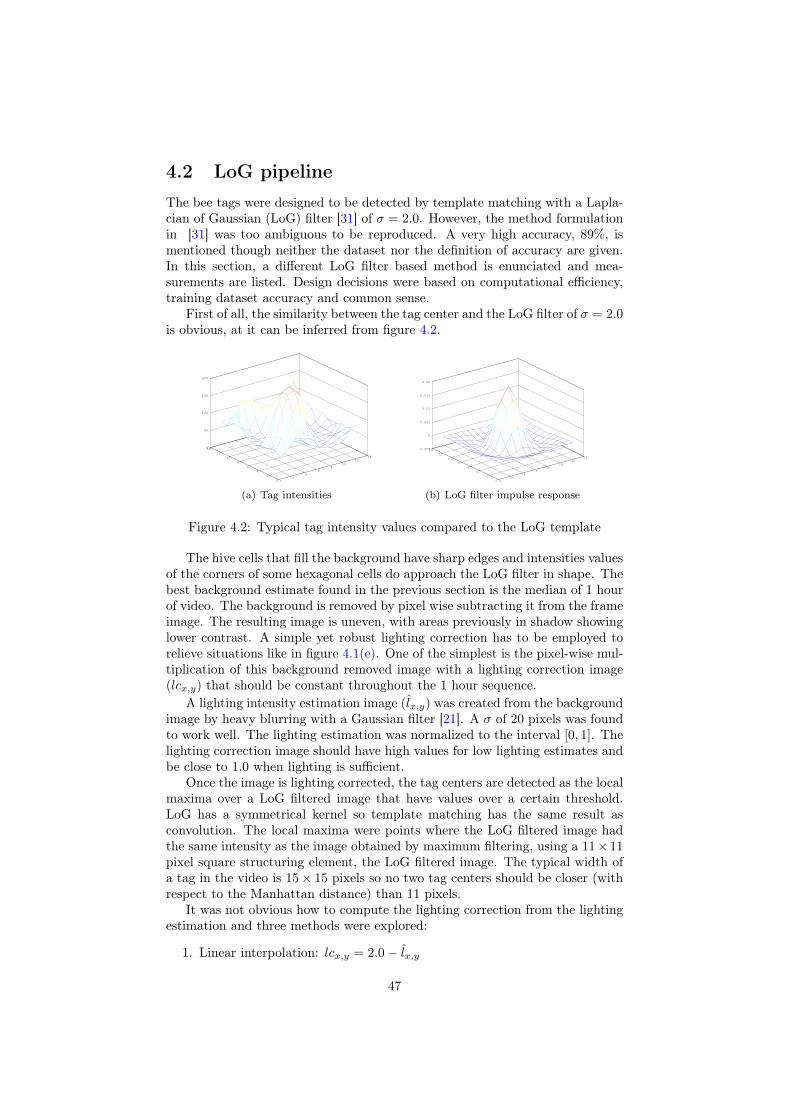
4.2 LoG pipelineThe bee tags were designed to be detected by template matching with a Lapla-cian of Gaussian (LoG) filter [31] of σ = 2.0. However, the method formulationin [31] was too ambiguous to be reproduced. A very high accuracy, 89%, ismentioned though neither the dataset nor the definition of accuracy are given.In this section, a different LoG filter based method is enunciated and mea-surements are listed. Design decisions were based on computational efficiency,training dataset accuracy and common sense.
First of all, the similarity between the tag center and the LoG filter of σ = 2.0is obvious, at it can be inferred from figure 4.2.
0
2
4
6
8
10
12
14
0
2
4
6
8
10
12
140
50
100
150
200
(a) Tag intensities0
2
4
6
8
10
12
14
0
2
4
6
8
10
12
14-0.005
0
0.005
0.01
0.015
0.02
(b) LoG filter impulse response
Figure 4.2: Typical tag intensity values compared to the LoG template
The hive cells that fill the background have sharp edges and intensities valuesof the corners of some hexagonal cells do approach the LoG filter in shape. Thebest background estimate found in the previous section is the median of 1 hourof video. The background is removed by pixel wise subtracting it from the frameimage. The resulting image is uneven, with areas previously in shadow showinglower contrast. A simple yet robust lighting correction has to be employed torelieve situations like in figure 4.1(e). One of the simplest is the pixel-wise mul-tiplication of this background removed image with a lighting correction image(lcx,y) that should be constant throughout the 1 hour sequence.
A lighting intensity estimation image (lx,y) was created from the backgroundimage by heavy blurring with a Gaussian filter [21]. A σ of 20 pixels was foundto work well. The lighting estimation was normalized to the interval [0, 1]. Thelighting correction image should have high values for low lighting estimates andbe close to 1.0 when lighting is sufficient.
Once the image is lighting corrected, the tag centers are detected as the localmaxima over a LoG filtered image that have values over a certain threshold.LoG has a symmetrical kernel so template matching has the same result asconvolution. The local maxima were points where the LoG filtered image hadthe same intensity as the image obtained by maximum filtering, using a 11× 11pixel square structuring element, the LoG filtered image. The typical width ofa tag in the video is 15× 15 pixels so no two tag centers should be closer (withrespect to the Manhattan distance) than 11 pixels.
It was not obvious how to compute the lighting correction from the lightingestimation and three methods were explored:
1. Linear interpolation: lcx,y = 2.0− lx,y
47
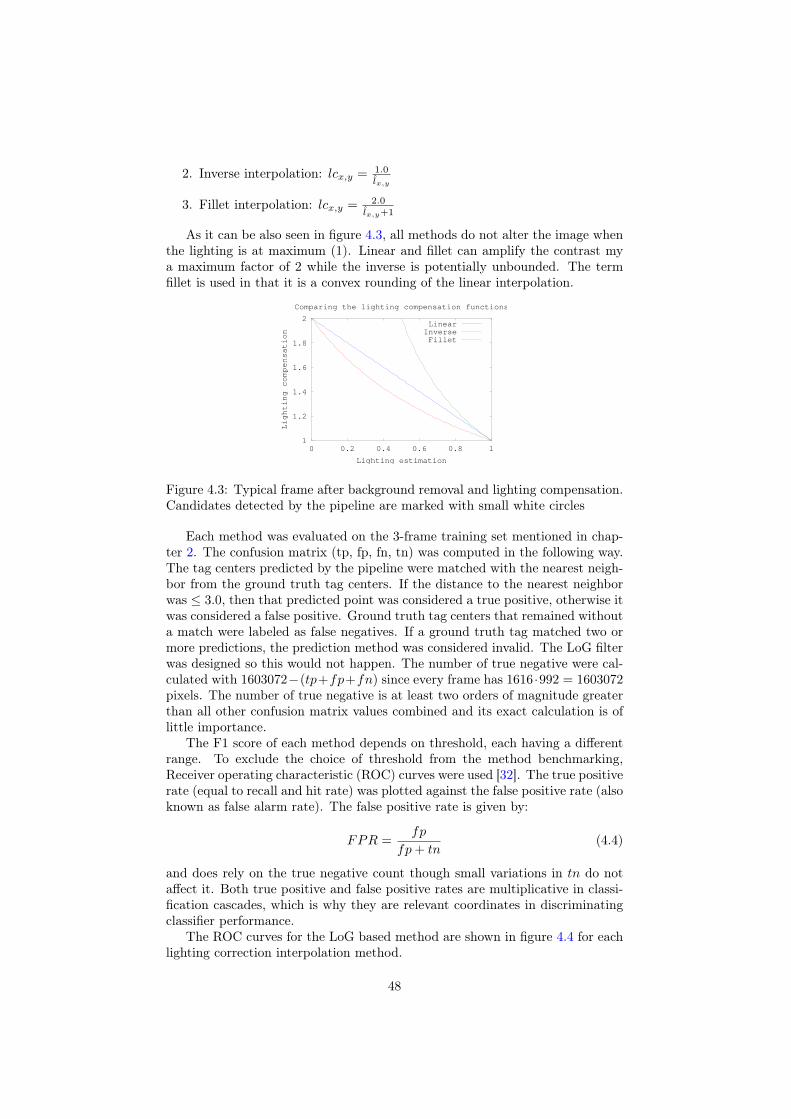
2. Inverse interpolation: lcx,y = 1.0lx,y
3. Fillet interpolation: lcx,y = 2.0lx,y+1
As it can be also seen in figure 4.3, all methods do not alter the image whenthe lighting is at maximum (1). Linear and fillet can amplify the contrast mya maximum factor of 2 while the inverse is potentially unbounded. The termfillet is used in that it is a convex rounding of the linear interpolation.
1
1.2
1.4
1.6
1.8
2
0 0.2 0.4 0.6 0.8 1
Lighting compensation
Lighting estimation
Comparing the lighting compensation functions
LinearInverseFillet
Figure 4.3: Typical frame after background removal and lighting compensation.Candidates detected by the pipeline are marked with small white circles
Each method was evaluated on the 3-frame training set mentioned in chap-ter 2. The confusion matrix (tp, fp, fn, tn) was computed in the following way.The tag centers predicted by the pipeline were matched with the nearest neigh-bor from the ground truth tag centers. If the distance to the nearest neighborwas ≤ 3.0, then that predicted point was considered a true positive, otherwise itwas considered a false positive. Ground truth tag centers that remained withouta match were labeled as false negatives. If a ground truth tag matched two ormore predictions, the prediction method was considered invalid. The LoG filterwas designed so this would not happen. The number of true negative were cal-culated with 1603072−(tp+fp+fn) since every frame has 1616 ·992 = 1603072pixels. The number of true negative is at least two orders of magnitude greaterthan all other confusion matrix values combined and its exact calculation is oflittle importance.
The F1 score of each method depends on threshold, each having a differentrange. To exclude the choice of threshold from the method benchmarking,Receiver operating characteristic (ROC) curves were used [32]. The true positiverate (equal to recall and hit rate) was plotted against the false positive rate (alsoknown as false alarm rate). The false positive rate is given by:
FPR =fp
fp+ tn(4.4)
and does rely on the true negative count though small variations in tn do notaffect it. Both true positive and false positive rates are multiplicative in classi-fication cascades, which is why they are relevant coordinates in discriminatingclassifier performance.
The ROC curves for the LoG based method are shown in figure 4.4 for eachlighting correction interpolation method.
48
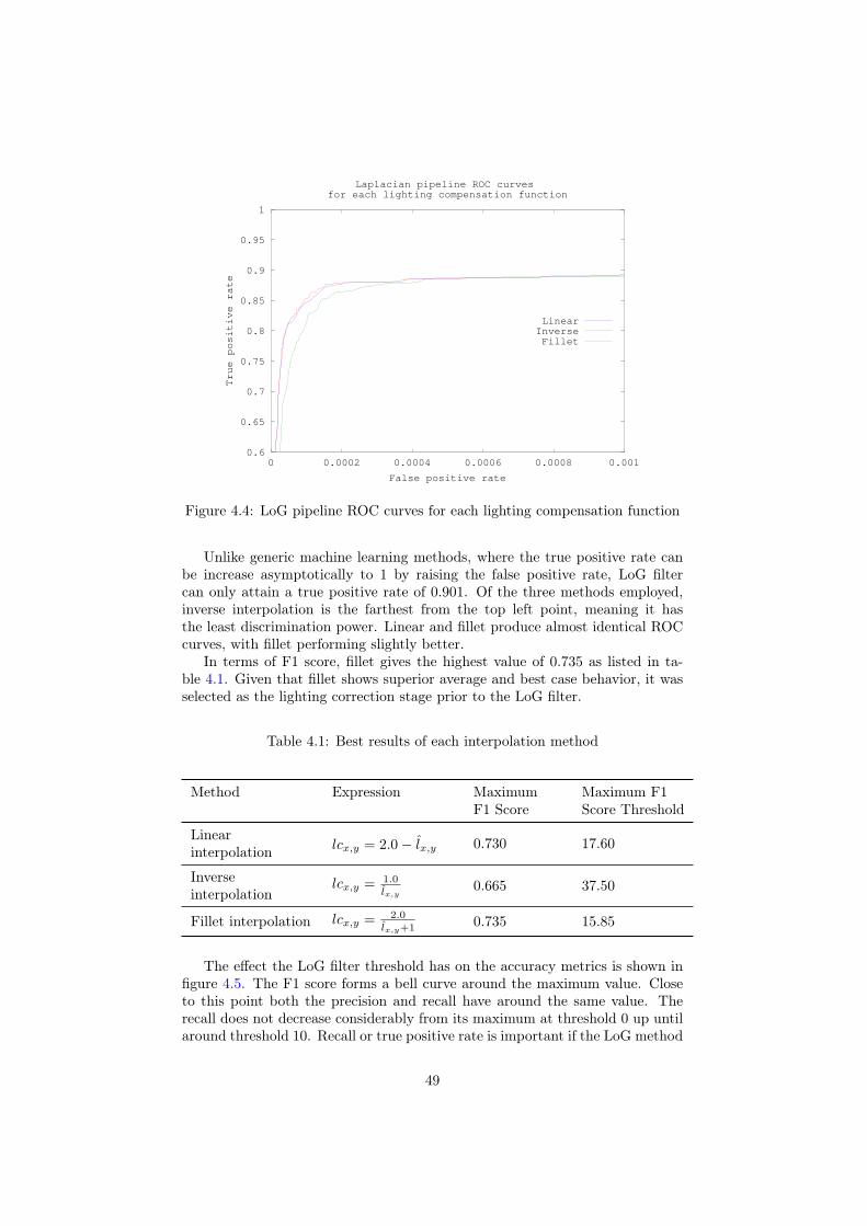
0.6
0.65
0.7
0.75
0.8
0.85
0.9
0.95
1
0 0.0002 0.0004 0.0006 0.0008 0.001
True positive rate
False positive rate
Laplacian pipeline ROC curves for each lighting compensation function
LinearInverseFillet
Figure 4.4: LoG pipeline ROC curves for each lighting compensation function
Unlike generic machine learning methods, where the true positive rate canbe increase asymptotically to 1 by raising the false positive rate, LoG filtercan only attain a true positive rate of 0.901. Of the three methods employed,inverse interpolation is the farthest from the top left point, meaning it hasthe least discrimination power. Linear and fillet produce almost identical ROCcurves, with fillet performing slightly better.
In terms of F1 score, fillet gives the highest value of 0.735 as listed in ta-ble 4.1. Given that fillet shows superior average and best case behavior, it wasselected as the lighting correction stage prior to the LoG filter.
Table 4.1: Best results of each interpolation method
Method Expression Maximum Maximum F1F1 Score Score Threshold
Linearinterpolation lcx,y = 2.0− lx,y 0.730 17.60
Inverseinterpolation
lcx,y = 1.0lx,y
0.665 37.50
Fillet interpolation lcx,y = 2.0lx,y+1 0.735 15.85
The effect the LoG filter threshold has on the accuracy metrics is shown infigure 4.5. The F1 score forms a bell curve around the maximum value. Closeto this point both the precision and recall have around the same value. Therecall does not decrease considerably from its maximum at threshold 0 up untilaround threshold 10. Recall or true positive rate is important if the LoG method
49
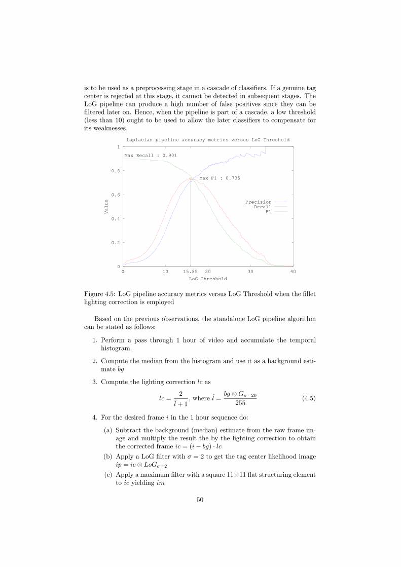
is to be used as a preprocessing stage in a cascade of classifiers. If a genuine tagcenter is rejected at this stage, it cannot be detected in subsequent stages. TheLoG pipeline can produce a high number of false positives since they can befiltered later on. Hence, when the pipeline is part of a cascade, a low threshold(less than 10) ought to be used to allow the later classifiers to compensate forits weaknesses.
0
0.2
0.4
0.6
0.8
1
0 10 15.85 20 30 40
Value
LoG Threshold
Laplacian pipeline accuracy metrics versus LoG Threshold
PrecisionRecall
F1
Max F1 : 0.735
Max Recall : 0.901
Figure 4.5: LoG pipeline accuracy metrics versus LoG Threshold when the filletlighting correction is employed
Based on the previous observations, the standalone LoG pipeline algorithmcan be stated as follows:
1. Perform a pass through 1 hour of video and accumulate the temporalhistogram.
2. Compute the median from the histogram and use it as a background esti-mate bg
3. Compute the lighting correction lc as
lc =2
l + 1, where l =
bg ⊗Gσ=20
255(4.5)
4. For the desired frame i in the 1 hour sequence do:
(a) Subtract the background (median) estimate from the raw frame im-age and multiply the result the by the lighting correction to obtainthe corrected frame ic = (i− bg) · lc
(b) Apply a LoG filter with σ = 2 to get the tag center likelihood imageip = ic⊗ LoGσ=2
(c) Apply a maximum filter with a square 11×11 flat structuring elementto ic yielding im
50
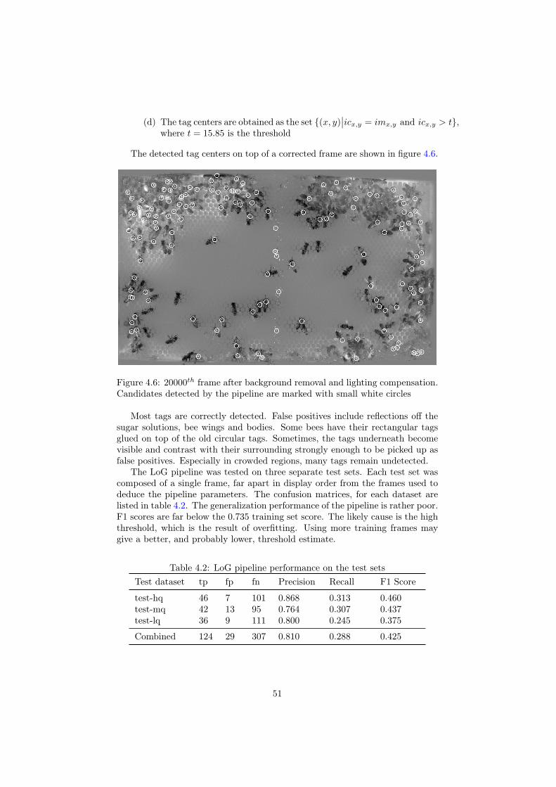
(d) The tag centers are obtained as the set {(x, y)∣∣icx,y = imx,y and icx,y > t},
where t = 15.85 is the threshold
The detected tag centers on top of a corrected frame are shown in figure 4.6.
Figure 4.6: 20000th frame after background removal and lighting compensation.Candidates detected by the pipeline are marked with small white circles
Most tags are correctly detected. False positives include reflections off thesugar solutions, bee wings and bodies. Some bees have their rectangular tagsglued on top of the old circular tags. Sometimes, the tags underneath becomevisible and contrast with their surrounding strongly enough to be picked up asfalse positives. Especially in crowded regions, many tags remain undetected.
The LoG pipeline was tested on three separate test sets. Each test set wascomposed of a single frame, far apart in display order from the frames used todeduce the pipeline parameters. The confusion matrices, for each dataset arelisted in table 4.2. The generalization performance of the pipeline is rather poor.F1 scores are far below the 0.735 training set score. The likely cause is the highthreshold, which is the result of overfitting. Using more training frames maygive a better, and probably lower, threshold estimate.
Table 4.2: LoG pipeline performance on the test setsTest dataset tp fp fn Precision Recall F1 Score
test-hq 46 7 101 0.868 0.313 0.460test-mq 42 13 95 0.764 0.307 0.437test-lq 36 9 111 0.800 0.245 0.375
Combined 124 29 307 0.810 0.288 0.425
51
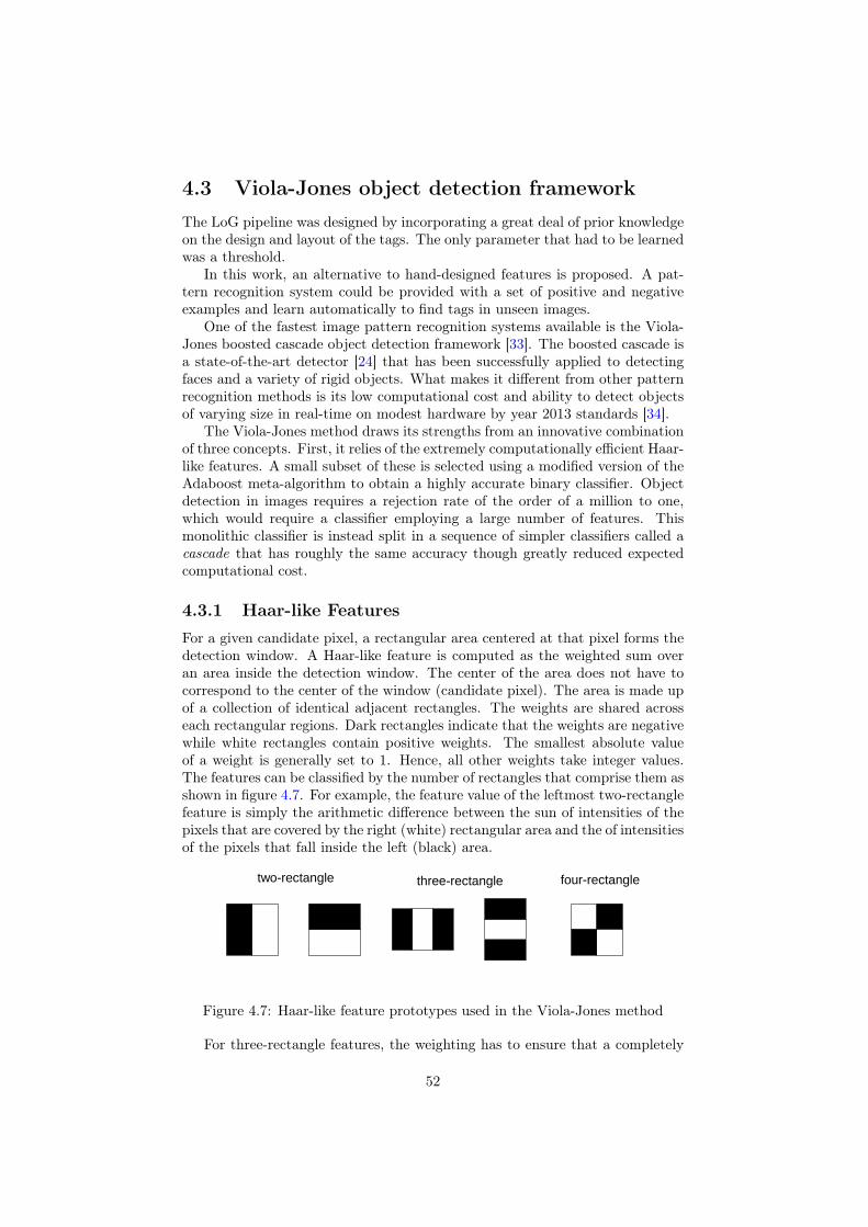
4.3 Viola-Jones object detection frameworkThe LoG pipeline was designed by incorporating a great deal of prior knowledgeon the design and layout of the tags. The only parameter that had to be learnedwas a threshold.
In this work, an alternative to hand-designed features is proposed. A pat-tern recognition system could be provided with a set of positive and negativeexamples and learn automatically to find tags in unseen images.
One of the fastest image pattern recognition systems available is the Viola-Jones boosted cascade object detection framework [33]. The boosted cascade isa state-of-the-art detector [24] that has been successfully applied to detectingfaces and a variety of rigid objects. What makes it different from other patternrecognition methods is its low computational cost and ability to detect objectsof varying size in real-time on modest hardware by year 2013 standards [34].
The Viola-Jones method draws its strengths from an innovative combinationof three concepts. First, it relies of the extremely computationally efficient Haar-like features. A small subset of these is selected using a modified version of theAdaboost meta-algorithm to obtain a highly accurate binary classifier. Objectdetection in images requires a rejection rate of the order of a million to one,which would require a classifier employing a large number of features. Thismonolithic classifier is instead split in a sequence of simpler classifiers called acascade that has roughly the same accuracy though greatly reduced expectedcomputational cost.
4.3.1 Haar-like FeaturesFor a given candidate pixel, a rectangular area centered at that pixel forms thedetection window. A Haar-like feature is computed as the weighted sum overan area inside the detection window. The center of the area does not have tocorrespond to the center of the window (candidate pixel). The area is made upof a collection of identical adjacent rectangles. The weights are shared acrosseach rectangular regions. Dark rectangles indicate that the weights are negativewhile white rectangles contain positive weights. The smallest absolute valueof a weight is generally set to 1. Hence, all other weights take integer values.The features can be classified by the number of rectangles that comprise them asshown in figure 4.7. For example, the feature value of the leftmost two-rectanglefeature is simply the arithmetic difference between the sun of intensities of thepixels that are covered by the right (white) rectangular area and the of intensitiesof the pixels that fall inside the left (black) area.
two-rectangle three-rectangle four-rectangle
Figure 4.7: Haar-like feature prototypes used in the Viola-Jones method
For three-rectangle features, the weighting has to ensure that a completely
52
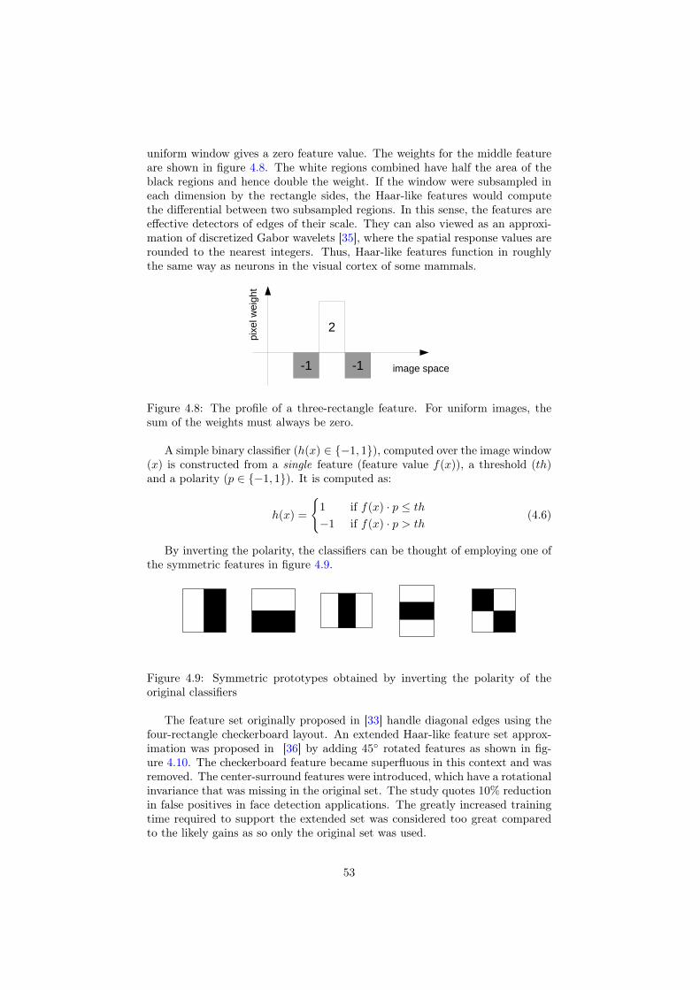
uniform window gives a zero feature value. The weights for the middle featureare shown in figure 4.8. The white regions combined have half the area of theblack regions and hence double the weight. If the window were subsampled ineach dimension by the rectangle sides, the Haar-like features would computethe differential between two subsampled regions. In this sense, the features areeffective detectors of edges of their scale. They can also viewed as an approxi-mation of discretized Gabor wavelets [35], where the spatial response values arerounded to the nearest integers. Thus, Haar-like features function in roughlythe same way as neurons in the visual cortex of some mammals.
2
-1 -1
pixe
l wei
ght
image space
Figure 4.8: The profile of a three-rectangle feature. For uniform images, thesum of the weights must always be zero.
A simple binary classifier (h(x) ∈ {−1, 1}), computed over the image window(x) is constructed from a single feature (feature value f(x)), a threshold (th)and a polarity (p ∈ {−1, 1}). It is computed as:
h(x) =
{1 if f(x) · p ≤ th−1 if f(x) · p > th
(4.6)
By inverting the polarity, the classifiers can be thought of employing one ofthe symmetric features in figure 4.9.
Figure 4.9: Symmetric prototypes obtained by inverting the polarity of theoriginal classifiers
The feature set originally proposed in [33] handle diagonal edges using thefour-rectangle checkerboard layout. An extended Haar-like feature set approx-imation was proposed in [36] by adding 45◦ rotated features as shown in fig-ure 4.10. The checkerboard feature became superfluous in this context and wasremoved. The center-surround features were introduced, which have a rotationalinvariance that was missing in the original set. The study quotes 10% reductionin false positives in face detection applications. The greatly increased trainingtime required to support the extended set was considered too great comparedto the likely gains as so only the original set was used.
53
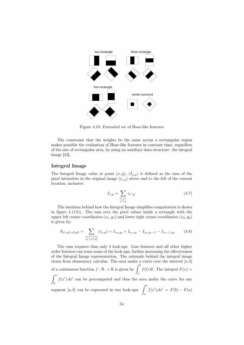
two-rectangle three-rectangle
four-rectangle
center-surround
Figure 4.10: Extended set of Haar-like features
The constraint that the weights be the same across a rectangular regionmakes possible the evaluation of Haar-like features in constant time, regardlessof the size of rectangular area, by using an auxiliary data structure: the integralimage [33].
Integral ImageThe Integral Image value at point (x, y), (Ix,y) is defined as the sum of thepixel intensities in the original image (ix,y) above and to the left of the currentlocation, inclusive:
Ix,y =∑x′≤xy′≤y
ix′,y′ (4.7)
The intuition behind how the Integral Image simplifies computation is shownin figure 4.11(b). The sum over the pixel values inside a rectangle with theupper left corner coordinates (x1, y1) and lower right corner coordinates (x2, y2)is given by:
Sx1,y1,x2,y2 =∑
x1≤x≤x2y1≤y≤y2
(ix,y) = Ix2,y2 + Ix1,y1 − Ix2,y1−1 − Ix1−1,y2 (4.8)
The sum requires thus only 4 look-ups. Line features and all other higherorder features can reuse some of the look-ups, further increasing the effectivenessof the Integral Image representation. The rationale behind the integral imagestems from elementary calculus. The area under a curve over the interval [a, b]
of a continuous function f : R→ R is given by∫ b
a
f(t) dt. The integral F (x) =∫ x
0
f(x′) dx′ can be precomputed and thus the area under the curve for any
segment [a, b] can be expressed in two look-ups:∫ b
a
f(x′) dx′ = F (b) − F (a)
54
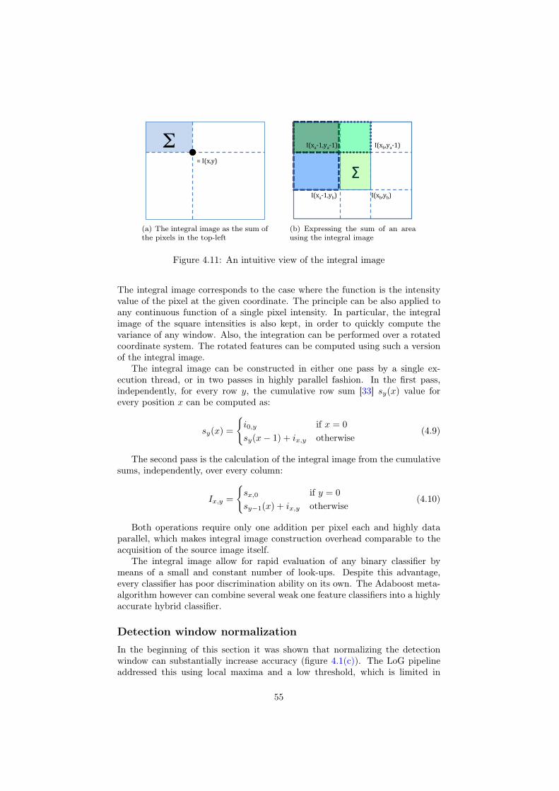
Σ = I(x,y)
(a) The integral image as the sum ofthe pixels in the top-left
Σ
I(xa-‐1,ya-‐1) I(xb,ya-‐1)
I(xb,yb) I(xa-‐1,yb)
(b) Expressing the sum of an areausing the integral image
Figure 4.11: An intuitive view of the integral image
The integral image corresponds to the case where the function is the intensityvalue of the pixel at the given coordinate. The principle can be also applied toany continuous function of a single pixel intensity. In particular, the integralimage of the square intensities is also kept, in order to quickly compute thevariance of any window. Also, the integration can be performed over a rotatedcoordinate system. The rotated features can be computed using such a versionof the integral image.
The integral image can be constructed in either one pass by a single ex-ecution thread, or in two passes in highly parallel fashion. In the first pass,independently, for every row y, the cumulative row sum [33] sy(x) value forevery position x can be computed as:
sy(x) =
{i0,y if x = 0
sy(x− 1) + ix,y otherwise(4.9)
The second pass is the calculation of the integral image from the cumulativesums, independently, over every column:
Ix,y =
{sx,0 if y = 0
sy−1(x) + ix,y otherwise(4.10)
Both operations require only one addition per pixel each and highly dataparallel, which makes integral image construction overhead comparable to theacquisition of the source image itself.
The integral image allow for rapid evaluation of any binary classifier bymeans of a small and constant number of look-ups. Despite this advantage,every classifier has poor discrimination ability on its own. The Adaboost meta-algorithm however can combine several weak one feature classifiers into a highlyaccurate hybrid classifier.
Detection window normalizationIn the beginning of this section it was shown that normalizing the detectionwindow can substantially increase accuracy (figure 4.1(c)). The LoG pipelineaddressed this using local maxima and a low threshold, which is limited in
55
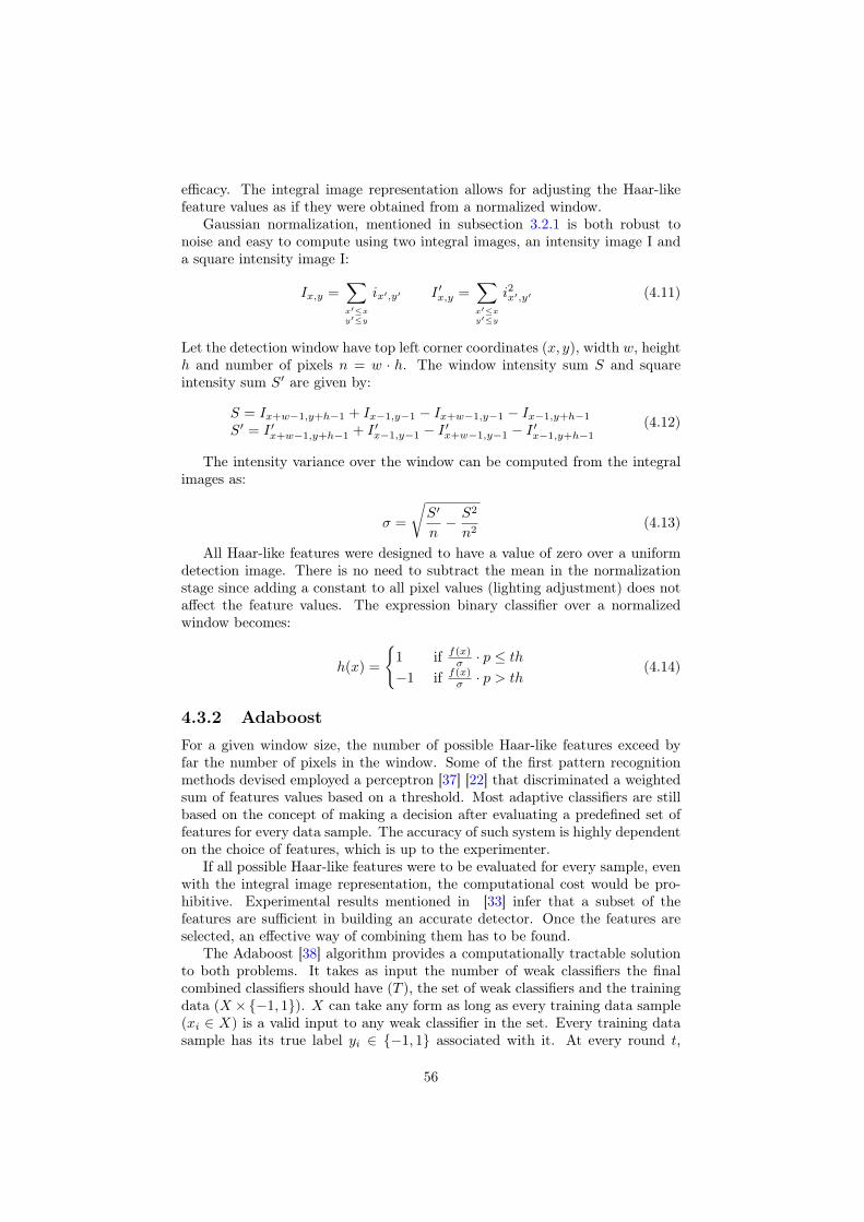
efficacy. The integral image representation allows for adjusting the Haar-likefeature values as if they were obtained from a normalized window.
Gaussian normalization, mentioned in subsection 3.2.1 is both robust tonoise and easy to compute using two integral images, an intensity image I anda square intensity image I:
Ix,y =∑x′≤xy′≤y
ix′,y′ I ′x,y =∑x′≤xy′≤y
i2x′,y′ (4.11)
Let the detection window have top left corner coordinates (x, y), width w, heighth and number of pixels n = w · h. The window intensity sum S and squareintensity sum S′ are given by:
S = Ix+w−1,y+h−1 + Ix−1,y−1 − Ix+w−1,y−1 − Ix−1,y+h−1
S′ = I ′x+w−1,y+h−1 + I ′x−1,y−1 − I ′x+w−1,y−1 − I ′x−1,y+h−1(4.12)
The intensity variance over the window can be computed from the integralimages as:
σ =
√S′
n− S2
n2(4.13)
All Haar-like features were designed to have a value of zero over a uniformdetection image. There is no need to subtract the mean in the normalizationstage since adding a constant to all pixel values (lighting adjustment) does notaffect the feature values. The expression binary classifier over a normalizedwindow becomes:
h(x) =
{1 if f(x)
σ · p ≤ th−1 if f(x)
σ · p > th(4.14)
4.3.2 AdaboostFor a given window size, the number of possible Haar-like features exceed byfar the number of pixels in the window. Some of the first pattern recognitionmethods devised employed a perceptron [37] [22] that discriminated a weightedsum of features values based on a threshold. Most adaptive classifiers are stillbased on the concept of making a decision after evaluating a predefined set offeatures for every data sample. The accuracy of such system is highly dependenton the choice of features, which is up to the experimenter.
If all possible Haar-like features were to be evaluated for every sample, evenwith the integral image representation, the computational cost would be pro-hibitive. Experimental results mentioned in [33] infer that a subset of thefeatures are sufficient in building an accurate detector. Once the features areselected, an effective way of combining them has to be found.
The Adaboost [38] algorithm provides a computationally tractable solutionto both problems. It takes as input the number of weak classifiers the finalcombined classifiers should have (T ), the set of weak classifiers and the trainingdata (X ×{−1, 1}). X can take any form as long as every training data sample(xi ∈ X) is a valid input to any weak classifier in the set. Every training datasample has its true label yi ∈ {−1, 1} associated with it. At every round t,
56
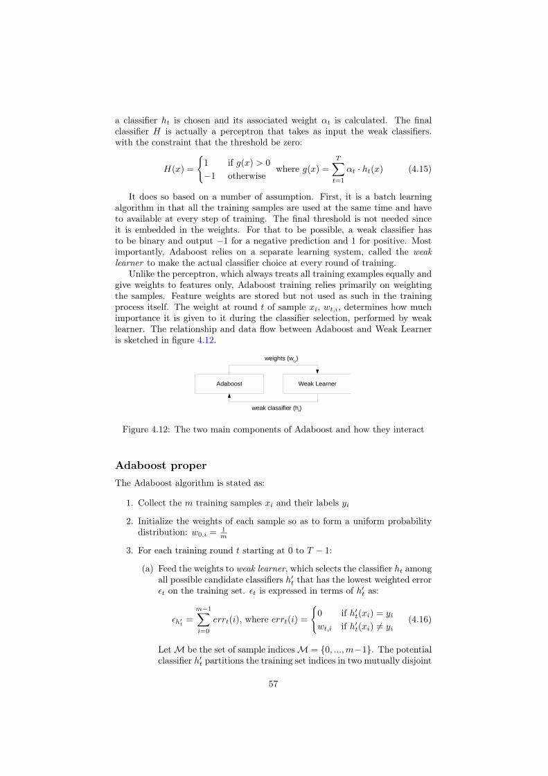
a classifier ht is chosen and its associated weight αt is calculated. The finalclassifier H is actually a perceptron that takes as input the weak classifiers.with the constraint that the threshold be zero:
H(x) =
{1 if g(x) > 0
−1 otherwisewhere g(x) =
T∑t=1
αt · ht(x) (4.15)
It does so based on a number of assumption. First, it is a batch learningalgorithm in that all the training samples are used at the same time and haveto available at every step of training. The final threshold is not needed sinceit is embedded in the weights. For that to be possible, a weak classifier hasto be binary and output −1 for a negative prediction and 1 for positive. Mostimportantly, Adaboost relies on a separate learning system, called the weaklearner to make the actual classifier choice at every round of training.
Unlike the perceptron, which always treats all training examples equally andgive weights to features only, Adaboost training relies primarily on weightingthe samples. Feature weights are stored but not used as such in the trainingprocess itself. The weight at round t of sample xi, wt,i, determines how muchimportance it is given to it during the classifier selection, performed by weaklearner. The relationship and data flow between Adaboost and Weak Learneris sketched in figure 4.12.
Adaboost Weak Learner
weights (wt,i)
weak classifier (ht)
Figure 4.12: The two main components of Adaboost and how they interact
Adaboost properThe Adaboost algorithm is stated as:
1. Collect the m training samples xi and their labels yi
2. Initialize the weights of each sample so as to form a uniform probabilitydistribution: w0,i = 1
m
3. For each training round t starting at 0 to T − 1:
(a) Feed the weights to weak learner, which selects the classifier ht amongall possible candidate classifiers h′t that has the lowest weighted errorεt on the training set. εt is expressed in terms of h′t as:
εh′t =
m−1∑i=0
errt(i), where errt(i) =
{0 if h′t(xi) = yi
wt,i if h′t(xi) 6= yi(4.16)
LetM be the set of sample indicesM = {0, ...,m−1}. The potentialclassifier h′t partitions the training set indices in two mutually disjoint
57
subsetsM = OKh′t
⋃NGh′t where
OKh′t= {i ∈ X
∣∣h′t(xi) = yi} andNGh′t = {i ∈ X
∣∣h′t(xi) 6= yi}(4.17)
OKh′tis the set of indices of the training samples that are correctly
predicted by h′t while NGh′t is the set of those incorrectly predicted.Since all the error terms in OKh′t
are zero, the weighted error of h′tcan be expressed as:
εh′t =∑
i∈NGh′t
wt,i (4.18)
The simplified notation OKt = OKht and NGt = NGht is used forthe partition created by ht.
(b) The correctly classified sample weights are decreased by multiplyingthem with a constant factor 0 < βt < 1 while the misclassified sampleweights are increased by multiplying with 1
βt:
w′t,i =
{wt,i ∗ βt if i ∈ OKt
wt,i ∗ 1βt
if i ∈ NGt(4.19)
The resulting weights are normalized in order to form a probabilitydistribution over the training set. The normalization term normt isgiven by:
normt =∑i∈M
w′t,i (4.20)
and the weights of the next round are obtained using:
wt+1,i =w′t,inormt
(4.21)
Intuitively, it makes sense that future classifiers should focus moreon the samples that could not be predicted correctly by the previ-ous classifiers in order to augment their strength. This also avoidselecting the same classifier.
4. Construct a confidence measure g that is a linear combination of the clas-
sifiers chosen at each round: g(x) =
T−1∑t=0
αt · ht(x)
5. The final classifier is simply the sign of the confidence measure: H(x) =sign(g(x))
The βt values have to be chosen as to prevent the same classifier from beingselected again. The weighted error ε′t on the new weights wt+1i of the classifierht must be as good as random guessing [39]:
ε′t =∑i∈NGt
wt+1,i =1
2(4.22)
58
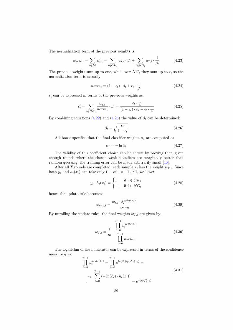
The normalization term of the previous weights is:
normt =∑i∈M
w′t,i =∑i∈OKt
wt,i · βt +∑i∈NGt
wt,i ·1
βt(4.23)
The previous weights sum up to one, while over NGt they sum up to εt so thenormalization term is actually:
normt = (1− εt) · βt + εt ·1
βt(4.24)
ε′t can be expressed in terms of the previous weights as:
ε′t =∑i∈NGt
wt,inormt
· βt =εt · 1
βt
(1− εt) · βt + εt · 1βt
(4.25)
By combining equations (4.22) and (4.25) the value of βt can be determined:
βt =
√εt
1− εt(4.26)
Adaboost specifies that the final classifier weights αt are computed as
αt = − lnβt (4.27)
The validity of this coefficient choice can be shown by proving that, givenenough rounds where the chosen weak classifiers are marginally better thanrandom guessing, the training error can be made arbitrarily small [40].
After all T rounds are completed, each sample xi has the weight wT,i. Sinceboth yi and ht(xi) can take only the values −1 or 1, we have:
yi · ht(xi) =
{1 if i ∈ OKt
−1 if i ∈ NGt(4.28)
hence the update rule becomes:
wt+1,i =wt,i · βyi·ht(xi)t
normt(4.29)
By unrolling the update rules, the final weights wT,i are given by:
wT,i =1
m·
T−1∏t=0
βyi·ht(xi)t
T−1∏t=0
normt
(4.30)
The logarithm of the numerator can be expressed in terms of the confidencemeasure g as:
T−1∏t=0
βyi·ht(xi)t =
T−1∏t=0
eln(βt)·yi·ht(xi) =
e
−yi·
T−1∑t=0
(− ln(βt) · ht(xi))= e−yi·f(xi)
(4.31)
59
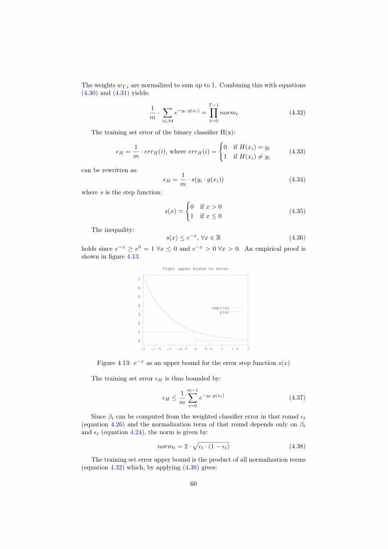
The weights wT,i are normalized to sum up to 1. Combining this with equations(4.30) and (4.31) yields:
1
m·∑i∈M
e−yi·g(xi) =
T−1∏t=0
normt (4.32)
The training set error of the binary classifier H(x):
εH =1
m· errH(i), where errH(i) =
{0 if H(xi) = yi
1 if H(xi) 6= yi(4.33)
can be rewritten as:εH =
1
m· s(yi · g(xi)) (4.34)
where s is the step function:
s(x) =
{0 if x > 0
1 if x ≤ 0(4.35)
The inequality:s(x) ≤ e−x, ∀x ∈ R (4.36)
holds since e−x ≥ e0 = 1 ∀x ≤ 0 and e−x > 0 ∀x > 0. An empirical proof isshown in figure 4.13.
0
1
2
3
4
5
6
7
-2 -1.5 -1 -0.5 0 0.5 1 1.5 2
Tight upper bound on error
exp(-x)s(x)
Figure 4.13: e−x as an upper bound for the error step function s(x)
The training set error εH is thus bounded by:
εH ≤1
m˙
m−1∑i=0
e−yi·g(xi) (4.37)
Since βt can be computed from the weighted classifier error in that round εt(equation 4.26) and the normalization term of that round depends only on βtand εt (equation 4.24), the norm is given by:
normt = 2 ·√εt · (1− εt) (4.38)
The training set error upper bound is the product of all normalization terms(equation 4.32) which, by applying (4.38) gives:
60
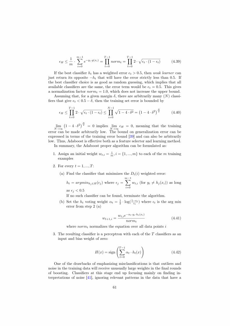
εH ≤1
m·m−1∑i=0
e−yi·g(xi) =
T−1∏t=0
normt =
T−1∏t=0
2 ·√εt · (1− εt) (4.39)
If the best classifier ht has a weighted error et > 0.5, then weak learner canjust return its opposite −ht that will have the error strictly less than 0.5. Ifthe best classifier choice is as good as random guessing, which implies that allavailable classifiers are the same, the error term would be et = 0.5. This givesa normalization factor normt = 1.0, which does not increase the upper bound.
Assuming that, for a given margin δ, there are arbitrarily many (N) classi-fiers that give et < 0.5− δ, then the training set error is bounded by
εH ≤T−1∏t=0
2 ·√εt · (1− εt) ≤
N−1∏i=0
√1− 4 · δ2 =
(1− 4 · δ2
)N2 (4.40)
limN→∞
(1− 4 · δ2
)N2 = 0 implies lim
N→∞εH = 0, meaning that the training
error can be made arbitrarily low. The bound on generalization error can beexpressed in terms of the training error bound [39] and can also be arbitrarilylow. Thus, Adaboost is effective both as a feature selector and learning method.
In summary, the Adaboost proper algorithm can be formulated as:
1. Assign an initial weight wt,i = 1m , i = {1, ...,m} to each of the m training
examples
2. For every t = 1, ..., T :
(a) Find the classifier that minimizes the Dt(i) weighted error:
ht = argminhj∈H(εj) where εj =
m−1∑i=0
wt,i (for yi 6= hj(xi)) as long
as εj < 0.5
If no such classifier can be found, terminate the algorithm.(b) Set the ht voting weight αt = 1
2 · log( 1−εtεt
) where εt is the arg minerror from step 2 (a)
wt+1,i =wt,ie
−αt·yi·ht(xi)
normt(4.41)
where normt normalizes the equation over all data points i
3. The resulting classifier is a perceptron with each of the T classifiers as aninput and bias weight of zero:
H(x) = sign
(T−1∑t=0
αt · ht(x)
)(4.42)
One of the drawbacks of emphasizing misclassifications is that outliers andnoise in the training data will receive unusually large weights in the final roundsof boosting. Classifiers at this stage end up focusing mainly on finding in-terpretations of noise [41], ignoring relevant patterns in the data that have a
61
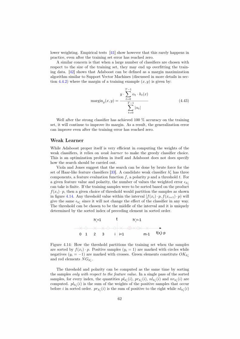
lower weighting. Empirical tests [41] show however that this rarely happens inpractice, even after the training set error has reached zero.
A similar concern is that when a large number of classifiers are chosen withrespect to the size of the training set, they may end up overfitting the train-ing data. [42] shows that Adaboost can be defined as a margin maximizationalgorithm similar to Support Vector Machines (discussed in more details in sec-tion 4.4.2) where the margin of a training example (x, y) is given by:
marging(x, y) =
y ·T−1∑t=0
αt · ht(x)
T−1∑t=0
|αt|
(4.43)
Well after the strong classifier has achieved 100 % accuracy on the trainingset, it will continue to improve its margin. As a result, the generalization errorcan improve even after the training error has reached zero.
Weak LearnerWhile Adaboost proper itself is very efficient in computing the weights of theweak classifiers, it relies on weak learner to make the greedy classifier choice.This is an optimization problem in itself and Adaboost does not does specifyhow the search should be carried out.
Viola and Jones suggest that the search can be done by brute force for theset of Haar-like feature classifiers [33]. A candidate weak classifier h′t has threecomponents, a feature evaluation function f , a polarity p and a threshold t. Fora given feature value and polarity, the number of values the weighted error εh′tcan take is finite. If the training samples were to be sorted based on the productf(xi) · p, then a given choice of threshold would partition the samples as shownin figure 4.14. Any threshold value within the interval [f(xi) · p, f(xi+1) · p) willgive the same εh′t since it will not change the effect of the classifier in any way.The threshold can be chosen to be the middle of the interval and it is uniquelydetermined by the sorted index of preceding element in sorted order.
t h't=-1h'
t=1
0 i+1i321 m-1 f(xi)∙
p
Figure 4.14: How the threshold partitions the training set when the samplesare sorted by f(xi) · p. Positive samples (yi = 1) are marked with circles whilenegatives (yi = −1) are marked with crosses. Green elements constitute OKh′tand red elements NGh′t .
The threshold and polarity can be computed as the same time by sortingthe samples only with respect to the feature value. In a single pass of the sortedsamples, for every index, the quantities plh′t(i), prh′t(i), nlh′t(i) and nrh′t(i) arecomputed. plh′t(i) is the sum of the weights of the positive samples that occurbefore i in sorted order. prh′t(i) is the sum of positive to the right while nlh′t(i)
62
and nrh′t(i) are the corresponding weight sums of negative samples. They aregiven by:
plh′t(i) =∑
j∈OKh′t , j≤iwt,j prh′t(i) =
∑j∈OKh′t , j>i
wt,j (4.44)
nlh′t(i) =∑
j∈NGh′t , j≤iwt,j nrh′t(i) =
∑j∈NGh′t , j>i
wt,j (4.45)
plh′t(i) and nlh′t(i) can be efficiently computed recursively, while prh′t(i) andnrh′t(i) can be expressed in terms of plh′t(i) and nlh′t(i):
prh′t(i) = plh′t(m− 1)− plh′t(i) (4.46)
nrh′t(i) = nlh′t(m− 1)− nlh′t(i) (4.47)
LetM be the set of the sorted indices. Two weighted errors are computed:
ε+h′t = mini∈M
plh′t(i) + nrh′t(i) (4.48)
ε−h′t = mini∈M
prh′t(i) + nlh′t(i) (4.49)
If ε+h′t is the smaller of the two, then the polarity is chosen to be p = 1. Otherwisethe polarity is reversed. The classifier error is ε′h′t = min(ε+h′t, ε
−h′t), This restricts
the search to occur only over all possible features and element indices. Boththe threshold and polarity can be inferred from these. The classifier returnedby weak learner is the one with the lowest error:
ht = arg minf∈F,i∈M
ε′h′t (4.50)
where F is the set of all possible features. The asymptotic complexity of weaklearner is, accounting for worst-case sorting performance, O(|F|·|M|· log(|M|).Since Adaboost calls weak learner exactly once per boosting round, the overalltraining complexity is: O(T · |F| · |M|· log(|M|). It is assumed that the featurescan be evaluated in constant time.
4.3.3 Boosted cascadeThe cascade concept assumes that for any subset of the training data W ,classifier can be trained to achieve a true positive rate greater than a pre-defined threshold TPRtarget and a false positive rate less than a predefinedFPRtarget. Let the set of all such classifiers be CW . A classifier of this kindthat is trained on the entire training data c0, can act as a filter. W is theset of all available training samples x ∈ X along with their labels y ∈ −1, 1,W = {(x, y)
∣∣x ∈ X and y ∈ {−1, 1}}. Let P be the set actual positives inW , P = {(x, y)
∣∣(x, y) ∈ W and y = 1} and N be the set of actual negativesN = W \P . LetW0 the set of all elements inW that are marked positive by c0,W0 = {(x, y)
∣∣(x, y) ∈ W and c0(x) = 1}, P0 and N0 its positive and negativesubsets. The confusion matrix on the training set of c0 is:
tp0 = |P0| fp0 = |N0| (4.51)fn0 = |P | − |P0| tn0 = |N | − |N0| (4.52)
63
Considering the constraints on the true positive rate (recall) tpr0 and falsepositive rate fpr0:
tpr0 =tp
tp+ fn≥ TPRtarget fpr0 =
fp
fp+ tn≤ FPRtarget (4.53)
the following relations are obtained:
|P0| ≥ TPRtarget · |P | |N0| ≤ FPRtarget · |N | (4.54)
W0 can be used to train another classifier, c1 with a true positive rate greaterthan TPRtarget and a false positive rate less than FPRtarget on W0, yieldingW1 and P1. The process can be repeated yielding as cascade of n classifiersc0, ..., cn−1. Let Wk, Pk, Nk, tprk and fprk be defined similarly for any stagek, k ∈ {1, ..., n− 1}. Equation (4.54) holds:
|Pk| ≥ TPRtarget · |Pk−1| |Nk| ≤ FPRtarget · |Nk−1| (4.55)
Applying these relations recursively give bounds on the true positive rate tprand the false positive rate fpr of the entire cascade:
tpr ≥ TPRntarget fpr ≤ FPRntarget (4.56)
Thus, assuming that suitable classifiers can be found, the number of falsenegatives and false positive of the cascade be made arbitrarily small resultingan arbitrarily high accuracy on the training set.
It has also been proven that Adaboost can train an arbitrarily accuratestrong classifier with far more relaxed constraints. Unlike an Adaboost classifier,where all the weak classifiers have to be evaluated for all samples, the cascadecan reduce computation time remarkably.
On the training data, if a sample is negative x ∈ N , the likelihood thatit will be present after k classification stages is P (x ∈ NK) ≤ FPRktarget. Ifa sample is positive, it will at most be evaluated by all the classifiers in thecascade. Hence, the average number of calls freq(ck) of classifier ck a trainingsample is freq(ck) ≤ |P |
|W | + FPRktarget. The cascade is employed in situationswhere the number of positives is very small compared to the size of the trainingdata. In these cases, the computation cost reduction is exceptional.
For instance, if the FPRtarget = 0.5 and the number of positives in thetraining data negligible, the average cost of evaluating a cascade made up ofclassifiers with identical computational complexity is less than of computingtwo classifiers for every data sample, irrespective of the number of classifiersemployed. Performance can be further tuned by selecting simpler classifiers forthe early stages of the cascade with very complex ones at the end.
Experimental results on face data imply that the cascade exhibits the samebehavior on unseen data [33] as on the training data making the cascade a validlearning method.
Cascade training
A cascade architecture requires classifiers with strict bounds on the true positiveand false positive rates. On the other hand, Adaboost produces classifier witharbitrarily high accuracy but does not offer any guarantees on the true positive
64
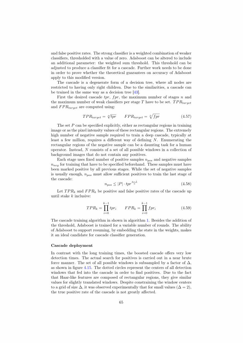
and false positive rates. The strong classifier is a weighted combination of weakerclassifiers, thresholded with a value of zero. Adaboost can be altered to includean additional parameter: the weighted sum threshold. This threshold can beadjusted to produce a classifier fit for a cascade. Further work needs to be donein order to prove whether the theoretical guarantees on accuracy of Adaboostapply to this modified version.
The cascade is a degenerate form of a decision tree, where all nodes arerestricted to having only right children. Due to the similarities, a cascade canbe trained in the same way as a decision tree [43].
First the desired cascade tpr, fpr, the maximum number of stages n andthe maximum number of weak classifiers per stage T have to be set. TPRtargetand FPRtarget are computed using:
TPRtarget = n√tpr FPRtarget = n
√fpr (4.57)
The set P can be specified explicitly, either as rectangular regions in trainingimage or as the pixel intensity values of these rectangular regions. The extremelyhigh number of negative sample required to train a deep cascade, typically atleast a few million, requires a different way of defining N . Enumerating therectangular regions of the negative sample can be a daunting task for a humanoperator. Instead, N consists of a set of all possible windows in a collection ofbackground images that do not contain any positives.
Each stage uses fixed number of positive samples npos and negative samplesnneg for training that have to be specified beforehand. These samples must havebeen marked positive by all previous stages. While the set of negative samplesis usually enough, npos must allow sufficient positives to train the last stage ofthe cascade:
npos ≤ |P | · tprn−1n (4.58)
Let TPRk and FPRk be positive and false positive rates of the cascade upuntil stake k inclusive:
TPRk =k−1∏i=0
tpri FPRk =k−1∏i=0
fpri (4.59)
The cascade training algorithm in shown in algorithm 1. Besides the addition ofthe threshold, Adaboost is trained for a variable number of rounds. The abilityof Adaboost to support resuming, by embedding the state in the weights, makesit an ideal candidate for cascade classifier generation.
Cascade deployment
In contrast with the long training times, the boosted cascade offers very lowdetection times. The actual search for positives is carried out in a near bruteforce manner. The set of all possible windows is subsampled by a factor of ∆,as shown in figure 4.15. The dotted circles represent the centers of all detectionwindows that fed into the cascade in order to find positives. Due to the factthat Haar-like features are composed of rectangular regions, they give similarvalues for slightly translated windows. Despite constraining the window centersto a grid of size ∆, it was observed experimentally that for small values (∆ = 2),the true positive rate of the cascade is not greatly affected.
65

Algorithm 1 Cascade trainingfor k = 0 to n− 1 do
Pk ← ∅ . Create training data for stage kwhile |Pk| < npos do . Obtain positives
Select xp ∈ Pif c0(xp) = 1 ... ck−1(xp) = 1 then
Pk ← Pk ∪ {xp}end if
end whileNk ← ∅ . Obtain negativesreject_countk ← 0while |Nk| < nneg do
Select a window xn ∈ Nif c0(xn) = 1 ... ck−1 = 1 then
Nk ← Nk ∪ {xn}else
reject_countk ← reject_countk + 1end if
end whileif nneg
reject_countk+nneg< FPR then
Terminate algorithmend ifWk ← Pk ∪Nkck ← empty classifier . Add a new stageInitialize weights w0,i over Wk according to Adaboostfor t = 0 to T − 1 do
Add weak classifier ht with weight αt to ck according to AdaboostAdjust weights w0,i according to Adaboostthreshold← 0while tpr(ck) < TPRtarget do
Decrease threshold
ck ← sign
t∑j=0
αj · hj
end whileif fpr(ck) = fprk ≤ FPRtarget then
Stop adding weak classifiers and break from this loopend if
end forend for
66
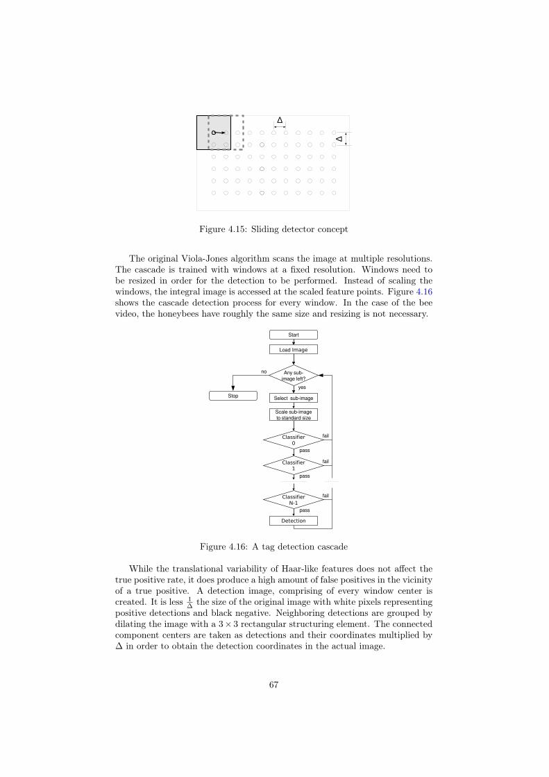
Δ
Δ
Figure 4.15: Sliding detector concept
The original Viola-Jones algorithm scans the image at multiple resolutions.The cascade is trained with windows at a fixed resolution. Windows need tobe resized in order for the detection to be performed. Instead of scaling thewindows, the integral image is accessed at the scaled feature points. Figure 4.16shows the cascade detection process for every window. In the case of the beevideo, the honeybees have roughly the same size and resizing is not necessary.
Start
Load Image
pass
Detection
Any sub-image left?
fail
Stop
Classifier 1
Classifier 0
Scale sub-image to standard size
Select sub-image
Classifier N-1
pass
pass
fail
fail
no
yes
Figure 4.16: A tag detection cascade
While the translational variability of Haar-like features does not affect thetrue positive rate, it does produce a high amount of false positives in the vicinityof a true positive. A detection image, comprising of every window center iscreated. It is less 1
∆ the size of the original image with white pixels representingpositive detections and black negative. Neighboring detections are grouped bydilating the image with a 3× 3 rectangular structuring element. The connectedcomponent centers are taken as detections and their coordinates multiplied by∆ in order to obtain the detection coordinates in the actual image.
67
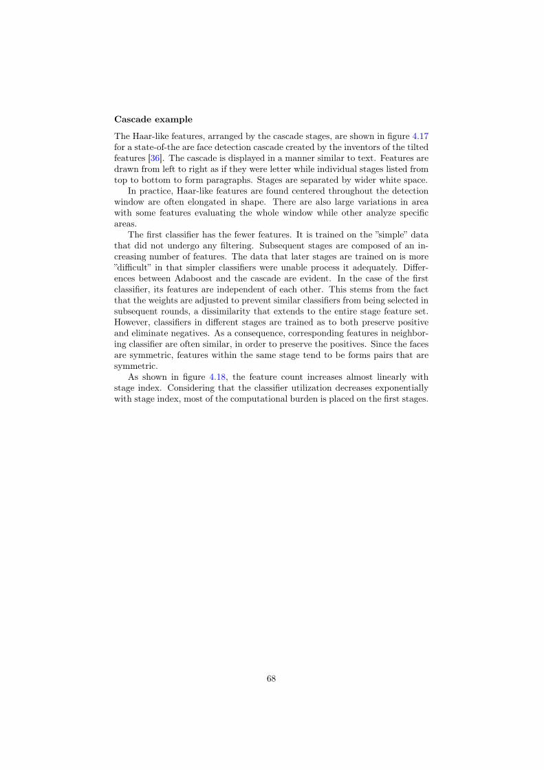
Cascade example
The Haar-like features, arranged by the cascade stages, are shown in figure 4.17for a state-of-the are face detection cascade created by the inventors of the tiltedfeatures [36]. The cascade is displayed in a manner similar to text. Features aredrawn from left to right as if they were letter while individual stages listed fromtop to bottom to form paragraphs. Stages are separated by wider white space.
In practice, Haar-like features are found centered throughout the detectionwindow are often elongated in shape. There are also large variations in areawith some features evaluating the whole window while other analyze specificareas.
The first classifier has the fewer features. It is trained on the ”simple” datathat did not undergo any filtering. Subsequent stages are composed of an in-creasing number of features. The data that later stages are trained on is more”difficult” in that simpler classifiers were unable process it adequately. Differ-ences between Adaboost and the cascade are evident. In the case of the firstclassifier, its features are independent of each other. This stems from the factthat the weights are adjusted to prevent similar classifiers from being selected insubsequent rounds, a dissimilarity that extends to the entire stage feature set.However, classifiers in different stages are trained as to both preserve positiveand eliminate negatives. As a consequence, corresponding features in neighbor-ing classifier are often similar, in order to preserve the positives. Since the facesare symmetric, features within the same stage tend to be forms pairs that aresymmetric.
As shown in figure 4.18, the feature count increases almost linearly withstage index. Considering that the classifier utilization decreases exponentiallywith stage index, most of the computational burden is placed on the first stages.
68
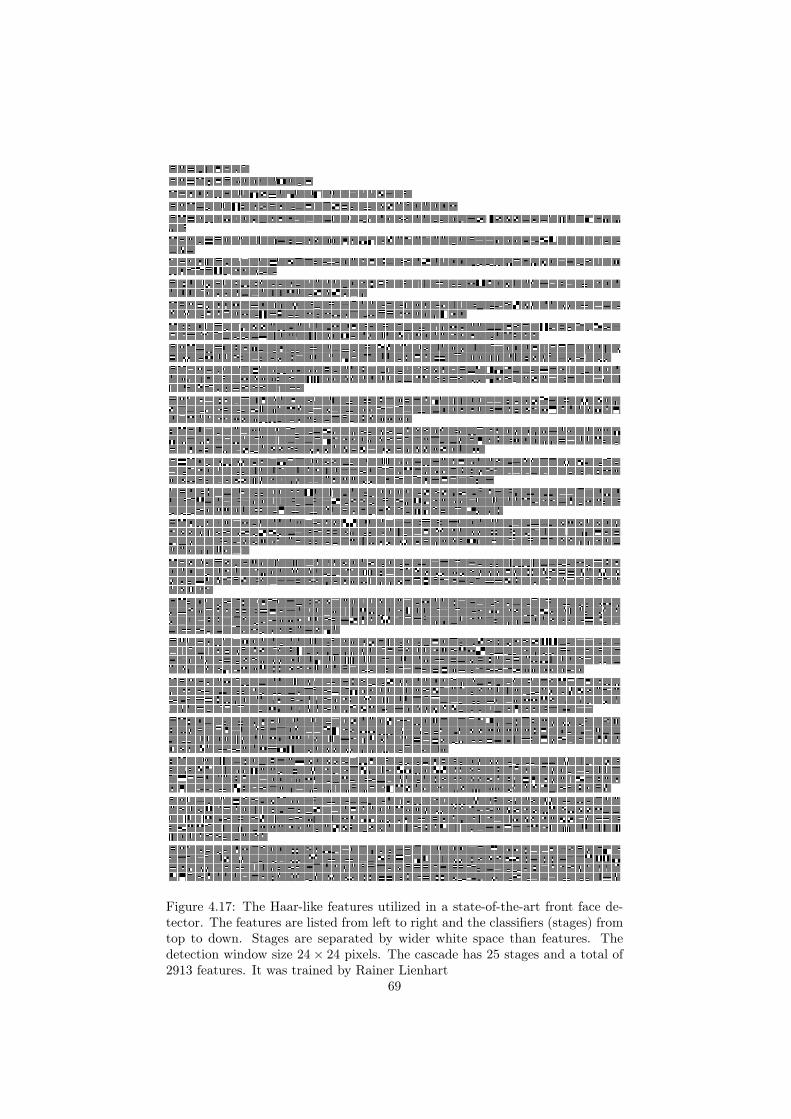
Figure 4.17: The Haar-like features utilized in a state-of-the-art front face de-tector. The features are listed from left to right and the classifiers (stages) fromtop to down. Stages are separated by wider white space than features. Thedetection window size 24× 24 pixels. The cascade has 25 stages and a total of2913 features. It was trained by Rainer Lienhart
69
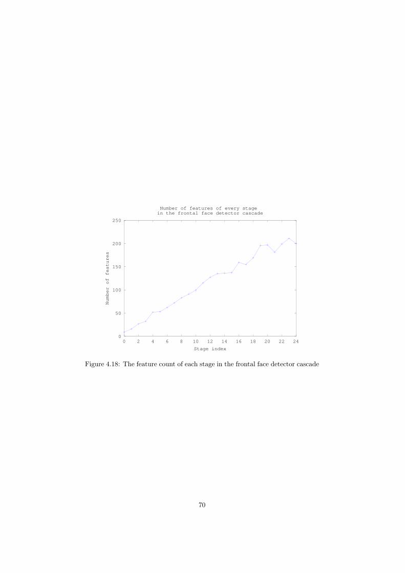
0
50
100
150
200
250
0 2 4 6 8 10 12 14 16 18 20 22 24
Number of features
Stage index
Number of features of every stage in the frontal face detector cascade
Figure 4.18: The feature count of each stage in the frontal face detector cascade
70
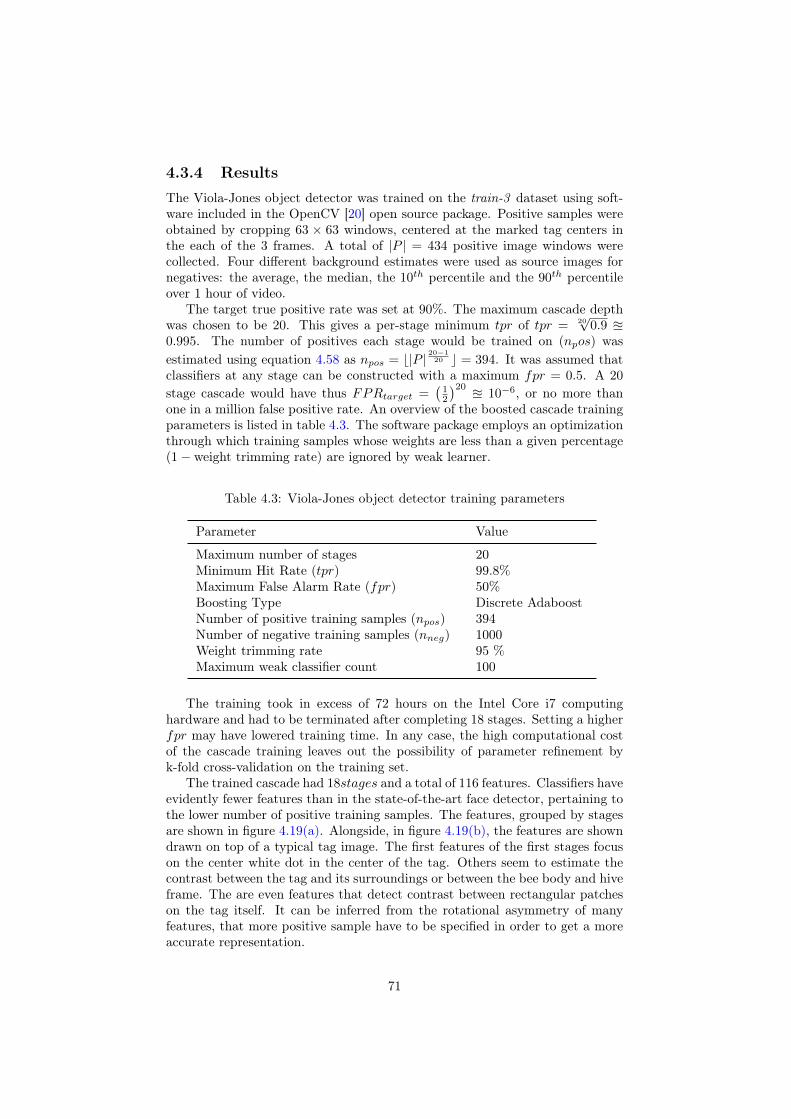
4.3.4 ResultsThe Viola-Jones object detector was trained on the train-3 dataset using soft-ware included in the OpenCV [20] open source package. Positive samples wereobtained by cropping 63 × 63 windows, centered at the marked tag centers inthe each of the 3 frames. A total of |P | = 434 positive image windows werecollected. Four different background estimates were used as source images fornegatives: the average, the median, the 10th percentile and the 90th percentileover 1 hour of video.
The target true positive rate was set at 90%. The maximum cascade depthwas chosen to be 20. This gives a per-stage minimum tpr of tpr = 20
√0.9 u
0.995. The number of positives each stage would be trained on (npos) wasestimated using equation 4.58 as npos = b|P | 20−1
20 c = 394. It was assumed thatclassifiers at any stage can be constructed with a maximum fpr = 0.5. A 20
stage cascade would have thus FPRtarget =(
12
)20 u 10−6, or no more thanone in a million false positive rate. An overview of the boosted cascade trainingparameters is listed in table 4.3. The software package employs an optimizationthrough which training samples whose weights are less than a given percentage(1− weight trimming rate) are ignored by weak learner.
Table 4.3: Viola-Jones object detector training parameters
Parameter Value
Maximum number of stages 20Minimum Hit Rate (tpr) 99.8%Maximum False Alarm Rate (fpr) 50%Boosting Type Discrete AdaboostNumber of positive training samples (npos) 394Number of negative training samples (nneg) 1000Weight trimming rate 95 %Maximum weak classifier count 100
The training took in excess of 72 hours on the Intel Core i7 computinghardware and had to be terminated after completing 18 stages. Setting a higherfpr may have lowered training time. In any case, the high computational costof the cascade training leaves out the possibility of parameter refinement byk-fold cross-validation on the training set.
The trained cascade had 18stages and a total of 116 features. Classifiers haveevidently fewer features than in the state-of-the-art face detector, pertaining tothe lower number of positive training samples. The features, grouped by stagesare shown in figure 4.19(a). Alongside, in figure 4.19(b), the features are showndrawn on top of a typical tag image. The first features of the first stages focuson the center white dot in the center of the tag. Others seem to estimate thecontrast between the tag and its surroundings or between the bee body and hiveframe. The are even features that detect contrast between rectangular patcheson the tag itself. It can be inferred from the rotational asymmetry of manyfeatures, that more positive sample have to be specified in order to get a moreaccurate representation.
71

(a) Boosted cascade Haar-like features (b) Boosted cascade Haar-like features su-perimposed on a typical tag image
Figure 4.19: Meaning of learned Haar-like features
Despite the apparent overfitting, the Viola-Jones cascade performs markedlybetter than the LoG pipeline on the single-frame test datasets. The confusionmatrices for every set are listed in table 4.4.
Table 4.4: Viola-Jones performance on the test sets
Test dataset tp fp fn Precision Recall F1 Score
test-hq 97 38 50 0.719 0.660 0.688test-mq 93 64 44 0.592 0.679 0.633test-lq 99 40 48 0.733 0.653 0.691
Combined 289 142 142 0.671 0.671 0.671
The detected tags in a typical frame (frame D) are shown in figure 4.20.The Gaussian normalization enable the cascade to detect tags in shadow. Someliquid splashes are mistakenly identified as they have a texture that is not presentin neither the positive nor the negative training samples.
72
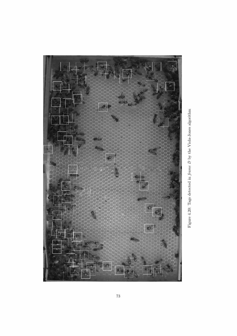
Figure4.20:Tagsdetected
infram
eD
bytheViola-Jon
esalgorithm
73
4.4 BenchmarksThe MNIST dataset is a popular means of evaluating the performance classi-fiers [44]. Among top performing methods on this dataset that do not requirepreprocessing and accept raw pixels as features are support vector machinesand multilayer perceptrons. Based on this evidence, both methods were chosenas benchmarks. Both methods have been covered extensively in the literature[45] [22], and will be explained only briefly. As black-box methods, they willbe evaluated based on their default specifications. Comprehensive study on thepotential of these methods is left for future research.
4.4.1 Multilayer perceptronsMultilayer perceptrons (MLP) are a form of neural networks that have shown aresurgence in popularity as a general purpose pattern recognition system [45].MLPs perform regression on a multidimensional input vector by mapping it toan output vector of (mostly) different dimensionality. The mapping consists ofa series of linear transformations (matrix multiplications), each followed by asigmoid squashing function. MLPs can be used in classification by roundingtheir output, often to a binary value. The most popular training algorithm forneural networks is gradient descent back-propagation [46]. It is based on thatfact that derivatives the objective function with respect to each weight (elementof a matrix), can be computed efficiently by performing the linear operationsin reverse order with the derivative of the sigmoid as a squashing function.Resilient propagation (RProp) [47] is an improvement on gradient descent thatuses an acceleration term and takes into account only the sign of the gradient.
4.4.2 Support vector machinesThe support vector machine (SVM) is a classification technique first introducedin [29]. It bears resemblance a Perceptron [22]. Given a set of points in highdimensional space, each marked with either a positive or negative label, the SVMstrives, just like the perceptron, to find a hyperplane that separates the positivesample from the negative samples. The perceptron convergence procedure stopswhen such a hyperplane was found. The SVM on the other hand, tries to findthe hyperplane that has a maximum margin, i.e. that maximizes the smallestdistance from any point in the space to it (figure 4.21). The points that havethis maximal margin distance, when projected onto the hyperplane form thesupport vectors, hence the name. Where the perceptron has potentially aninfinite number of possible viable solutions, the SVM has only one. The greaterthe margin, the more robust is SVM in generalization.
When the data points are not linearly separable (i.e. there is no hyperplanethat separates them), the perceptron fails to converge. The SVM instead adds apenalty term in its objective function for every misclassification. The objectivefunction combines margins with the penalty terms.
For very high dimensional spaces, a linear decision boundary is often suf-ficient [45]. There are cases, however, when accurate classification requires anon-linear boundary. The SVM calculates distances based on the definition ofthe dot product in the space. This definition can be altered algebraically towarp the space into an infinite dimensional space where a linear boundary can
74
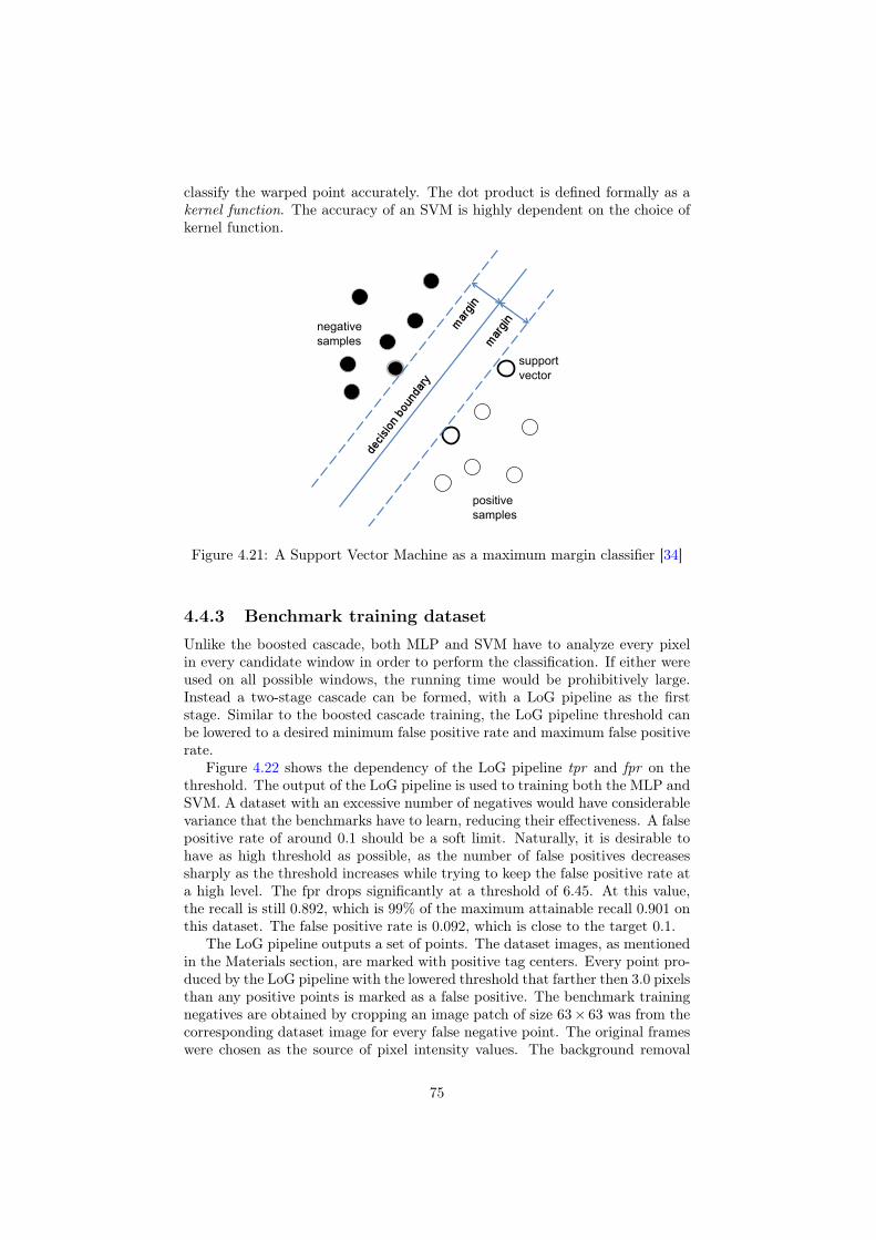
classify the warped point accurately. The dot product is defined formally as akernel function. The accuracy of an SVM is highly dependent on the choice ofkernel function.
positive samples
negative samples
support vector
Figure 4.21: A Support Vector Machine as a maximum margin classifier [34]
4.4.3 Benchmark training datasetUnlike the boosted cascade, both MLP and SVM have to analyze every pixelin every candidate window in order to perform the classification. If either wereused on all possible windows, the running time would be prohibitively large.Instead a two-stage cascade can be formed, with a LoG pipeline as the firststage. Similar to the boosted cascade training, the LoG pipeline threshold canbe lowered to a desired minimum false positive rate and maximum false positiverate.
Figure 4.22 shows the dependency of the LoG pipeline tpr and fpr on thethreshold. The output of the LoG pipeline is used to training both the MLP andSVM. A dataset with an excessive number of negatives would have considerablevariance that the benchmarks have to learn, reducing their effectiveness. A falsepositive rate of around 0.1 should be a soft limit. Naturally, it is desirable tohave as high threshold as possible, as the number of false positives decreasessharply as the threshold increases while trying to keep the false positive rate ata high level. The fpr drops significantly at a threshold of 6.45. At this value,the recall is still 0.892, which is 99% of the maximum attainable recall 0.901 onthis dataset. The false positive rate is 0.092, which is close to the target 0.1.
The LoG pipeline outputs a set of points. The dataset images, as mentionedin the Materials section, are marked with positive tag centers. Every point pro-duced by the LoG pipeline with the lowered threshold that farther then 3.0 pixelsthan any positive points is marked as a false positive. The benchmark trainingnegatives are obtained by cropping an image patch of size 63× 63 was from thecorresponding dataset image for every false negative point. The original frameswere chosen as the source of pixel intensity values. The background removal
75
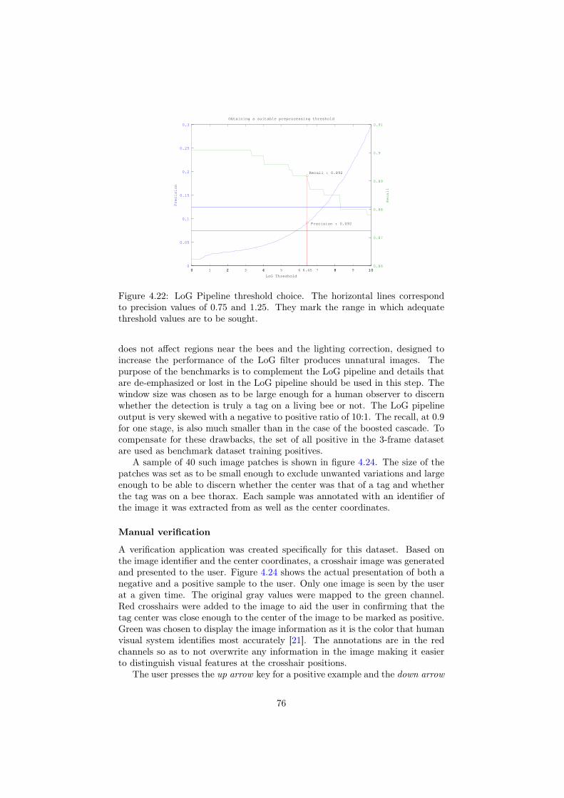
0
0.05
0.1
0.15
0.2
0.25
0.3
0 1 2 3 4 5 6.45 7 8 9 10
Precision
LoG Threshold
Precision : 0.092
0 2 4 6 8 100.86
0.87
0.88
0.89
0.9
0.91
Recall
Obtaining a suitable preprocessing threshold
Recall : 0.892
Figure 4.22: LoG Pipeline threshold choice. The horizontal lines correspondto precision values of 0.75 and 1.25. They mark the range in which adequatethreshold values are to be sought.
does not affect regions near the bees and the lighting correction, designed toincrease the performance of the LoG filter produces unnatural images. Thepurpose of the benchmarks is to complement the LoG pipeline and details thatare de-emphasized or lost in the LoG pipeline should be used in this step. Thewindow size was chosen as to be large enough for a human observer to discernwhether the detection is truly a tag on a living bee or not. The LoG pipelineoutput is very skewed with a negative to positive ratio of 10:1. The recall, at 0.9for one stage, is also much smaller than in the case of the boosted cascade. Tocompensate for these drawbacks, the set of all positive in the 3-frame datasetare used as benchmark dataset training positives.
A sample of 40 such image patches is shown in figure 4.24. The size of thepatches was set as to be small enough to exclude unwanted variations and largeenough to be able to discern whether the center was that of a tag and whetherthe tag was on a bee thorax. Each sample was annotated with an identifier ofthe image it was extracted from as well as the center coordinates.
Manual verification
A verification application was created specifically for this dataset. Based onthe image identifier and the center coordinates, a crosshair image was generatedand presented to the user. Figure 4.24 shows the actual presentation of both anegative and a positive sample to the user. Only one image is seen by the userat a given time. The original gray values were mapped to the green channel.Red crosshairs were added to the image to aid the user in confirming that thetag center was close enough to the center of the image to be marked as positive.Green was chosen to display the image information as it is the color that humanvisual system identifies most accurately [21]. The annotations are in the redchannels so as to not overwrite any information in the image making it easierto distinguish visual features at the crosshair positions.
The user presses the up arrow key for a positive example and the down arrow
76
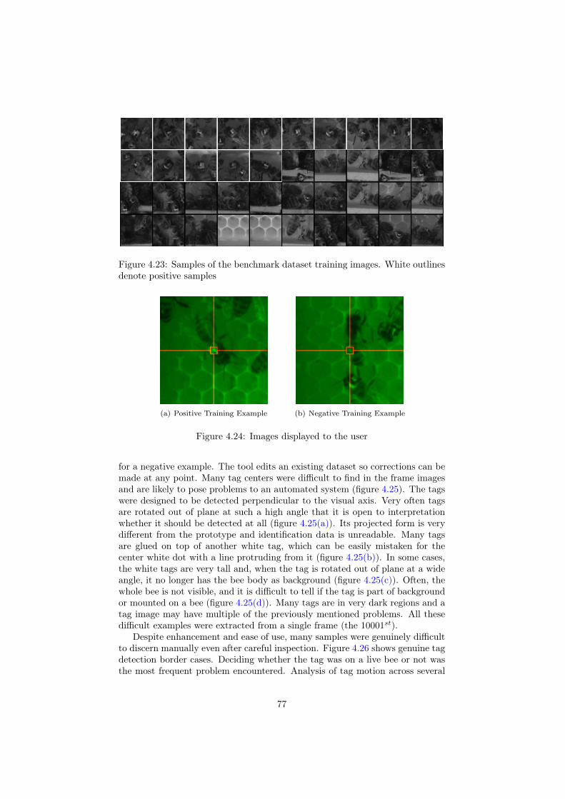
Figure 4.23: Samples of the benchmark dataset training images. White outlinesdenote positive samples
(a) Positive Training Example (b) Negative Training Example
Figure 4.24: Images displayed to the user
for a negative example. The tool edits an existing dataset so corrections can bemade at any point. Many tag centers were difficult to find in the frame imagesand are likely to pose problems to an automated system (figure 4.25). The tagswere designed to be detected perpendicular to the visual axis. Very often tagsare rotated out of plane at such a high angle that it is open to interpretationwhether it should be detected at all (figure 4.25(a)). Its projected form is verydifferent from the prototype and identification data is unreadable. Many tagsare glued on top of another white tag, which can be easily mistaken for thecenter white dot with a line protruding from it (figure 4.25(b)). In some cases,the white tags are very tall and, when the tag is rotated out of plane at a wideangle, it no longer has the bee body as background (figure 4.25(c)). Often, thewhole bee is not visible, and it is difficult to tell if the tag is part of backgroundor mounted on a bee (figure 4.25(d)). Many tags are in very dark regions and atag image may have multiple of the previously mentioned problems. All thesedifficult examples were extracted from a single frame (the 10001st).
Despite enhancement and ease of use, many samples were genuinely difficultto discern manually even after careful inspection. Figure 4.26 shows genuine tagdetection border cases. Deciding whether the tag was on a live bee or not wasthe most frequent problem encountered. Analysis of tag motion across several
77
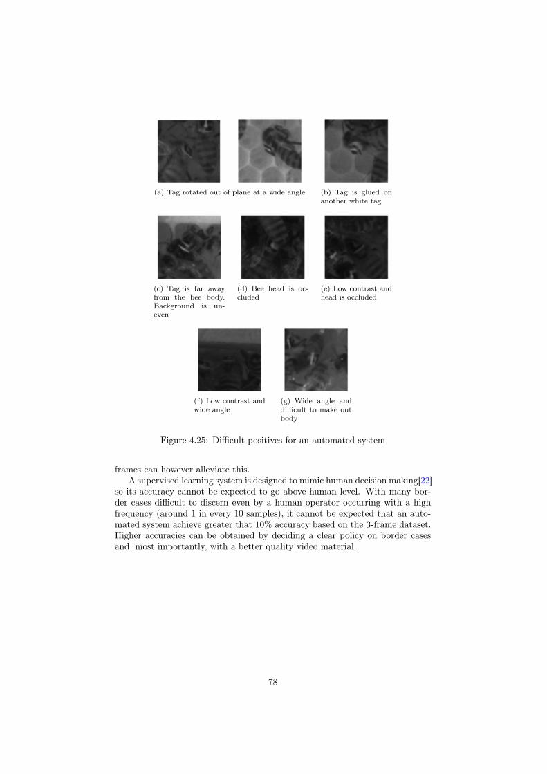
(a) Tag rotated out of plane at a wide angle (b) Tag is glued onanother white tag
(c) Tag is far awayfrom the bee body.Background is un-even
(d) Bee head is oc-cluded
(e) Low contrast andhead is occluded
(f) Low contrast andwide angle
(g) Wide angle anddifficult to make outbody
Figure 4.25: Difficult positives for an automated system
frames can however alleviate this.A supervised learning system is designed to mimic human decision making[22]
so its accuracy cannot be expected to go above human level. With many bor-der cases difficult to discern even by a human operator occurring with a highfrequency (around 1 in every 10 samples), it cannot be expected that an auto-mated system achieve greater that 10% accuracy based on the 3-frame dataset.Higher accuracies can be obtained by deciding a clear policy on border casesand, most importantly, with a better quality video material.
78
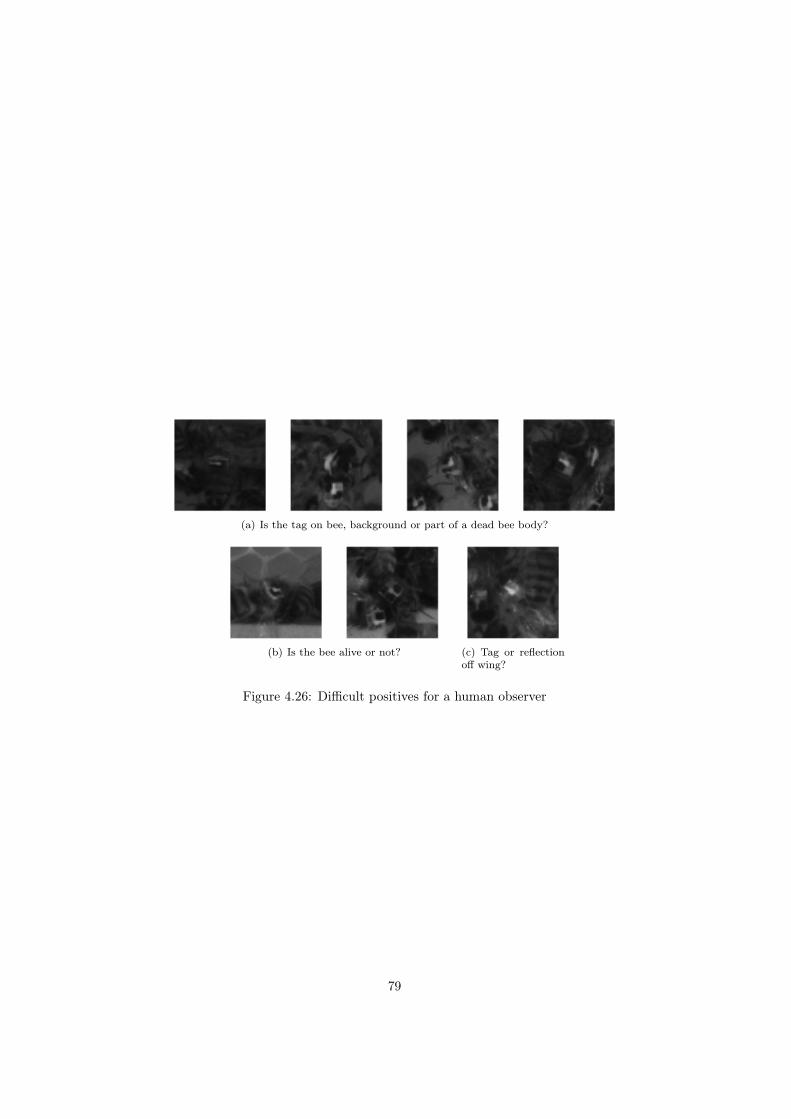
(a) Is the tag on bee, background or part of a dead bee body?
(b) Is the bee alive or not? (c) Tag or reflectionoff wing?
Figure 4.26: Difficult positives for a human observer
79
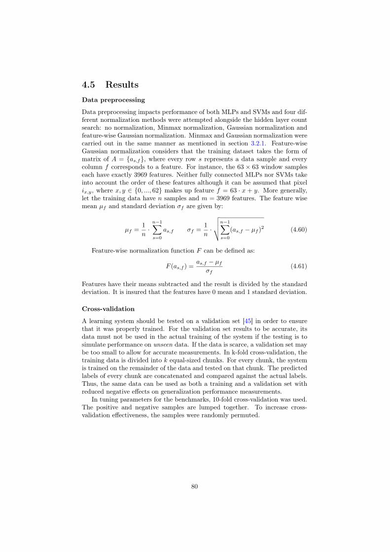
4.5 ResultsData preprocessing
Data preprocessing impacts performance of both MLPs and SVMs and four dif-ferent normalization methods were attempted alongside the hidden layer countsearch: no normalization, Minmax normalization, Gaussian normalization andfeature-wise Gaussian normalization. Minmax and Gaussian normalization werecarried out in the same manner as mentioned in section 3.2.1. Feature-wiseGaussian normalization considers that the training dataset takes the form ofmatrix of A = {as,f}, where every row s represents a data sample and everycolumn f corresponds to a feature. For instance, the 63 × 63 window sampleseach have exactly 3969 features. Neither fully connected MLPs nor SVMs takeinto account the order of these features although it can be assumed that pixelix,y, where x, y ∈ {0, ..., 62} makes up feature f = 63 · x + y. More generally,let the training data have n samples and m = 3969 features. The feature wisemean µf and standard deviation σf are given by:
µf =1
n·n−1∑s=0
as,f σf =1
n·
√√√√n−1∑s=0
(as,f − µf )2 (4.60)
Feature-wise normalization function F can be defined as:
F (as,f ) =as,f − µf
σf(4.61)
Features have their means subtracted and the result is divided by the standarddeviation. It is insured that the features have 0 mean and 1 standard deviation.
Cross-validation
A learning system should be tested on a validation set [45] in order to ensurethat it was properly trained. For the validation set results to be accurate, itsdata must not be used in the actual training of the system if the testing is tosimulate performance on unseen data. If the data is scarce, a validation set maybe too small to allow for accurate measurements. In k-fold cross-validation, thetraining data is divided into k equal-sized chunks. For every chunk, the systemis trained on the remainder of the data and tested on that chunk. The predictedlabels of every chunk are concatenated and compared against the actual labels.Thus, the same data can be used as both a training and a validation set withreduced negative effects on generalization performance measurements.
In tuning parameters for the benchmarks, 10-fold cross-validation was used.The positive and negative samples are lumped together. To increase cross-validation effectiveness, the samples were randomly permuted.
80
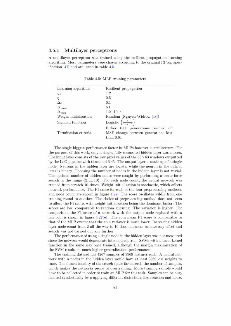
4.5.1 Multilayer perceptronsA multilayer perceptron was trained using the resilient propagation learningalgorithm. Most parameters were chosen according to the original RProp spec-ification [47] and are listed in table 4.5.
Table 4.5: MLP training parameters
Learning algorithm Resilient propagationη+ 1.2η− 0.5∆0 0.1∆max 50∆min 1.2 · 10−7
Weight initialization Random (Nguyen-Widrow [48])Sigmoid function Logistic
(1
1+e−x
)Termination criteria
Either 1000 generations reached orMSE change between generations lessthan 0.01
The single biggest performance factor in MLPs however is architecture. Forthe purpose of this work, only a single, fully connected hidden layer was chosen.The input layer consists of the raw pixel values of the 63×63 windows outputtedby the LoG pipeline with threshold 6.45. The output layer is made up of a singlenode. Neurons in the hidden layer are logistic while the neuron in the outputlater is binary. Choosing the number of nodes in the hidden layer is not trivial.The optimal number of hidden nodes were sought by performing a brute forcesearch in the range {2, ..., 10}. For each node count, the neural network wastrained from scratch 10 times. Weight initialization is stochastic, which affectsnetwork performance. The F1 score for each of the four preprocessing methodsand node count are shown in figure 4.27. The score oscillates wildly from onetraining round to another. The choice of preprocessing method does not seemto affect the F1 score, with weight initialization being the dominant factor. Thescores are low, comparable to random guessing. The variation is higher. Forcomparison, the F1 score of a network with the output node replaced with afair coin is shown in figure 4.27(e). The coin mean F1 score is comparable tothat of the MLP except that the coin variance is much lower. Increasing hiddenlayer node count from 2 all the way to 10 does not seem to have any effect andsearch was not carried out any further.
The performance of using a single node in the hidden layer was not measuredsince the network would degenerate into a perceptron. SVMs with a linear kernelfunction in the same way once trained, although the margin maximization ofthe SVM results in much higher generalization performance.
The training dataset has 4267 samples of 3969 features each. A neural net-work with n nodes in the hidden layer would have at least 3969× n weights totune. The dimensionality of the search space far exceeds the number of samples,which makes the networks prone to overtraining. More training sample wouldhave to be collected in order to train an MLP for this task. Samples can be aug-mented synthetically by a applying different distortions like rotation and noise.
81
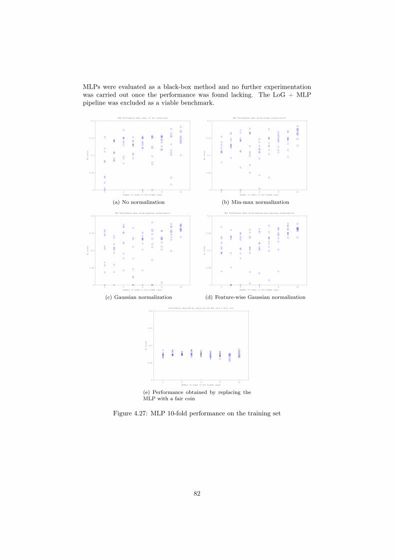
MLPs were evaluated as a black-box method and no further experimentationwas carried out once the performance was found lacking. The LoG + MLPpipeline was excluded as a viable benchmark.
0
0.05
0.1
0.15
0.2
2 4 6 8 10
F1 Score
Number of nodes in the hidden layer
MLP Performance when input is not normalized
(a) No normalization
0
0.05
0.1
0.15
0.2
2 4 6 8 10
F1 Score
Number of nodes in the hidden layer
MLP Performance when using minmax normalization
(b) Min-max normalization
0
0.05
0.1
0.15
0.2
2 4 6 8 10
F1 Score
Number of nodes in the hidden layer
MLP Performance when using Gaussian normalization
(c) Gaussian normalization
0
0.05
0.1
0.15
0.2
2 4 6 8 10
F1 Score
Number of nodes in the hidden layer
MLP Performance when using feature-wise Gaussian normalization
(d) Feature-wise Gaussian normalization
0
0.05
0.1
0.15
0.2
2 4 6 8 10
F1 Score
Number of nodes in the hidden layer
Performance obtained by replacing the MLP with a fair coin
(e) Performance obtained by replacing theMLP with a fair coin
Figure 4.27: MLP 10-fold performance on the training set
82
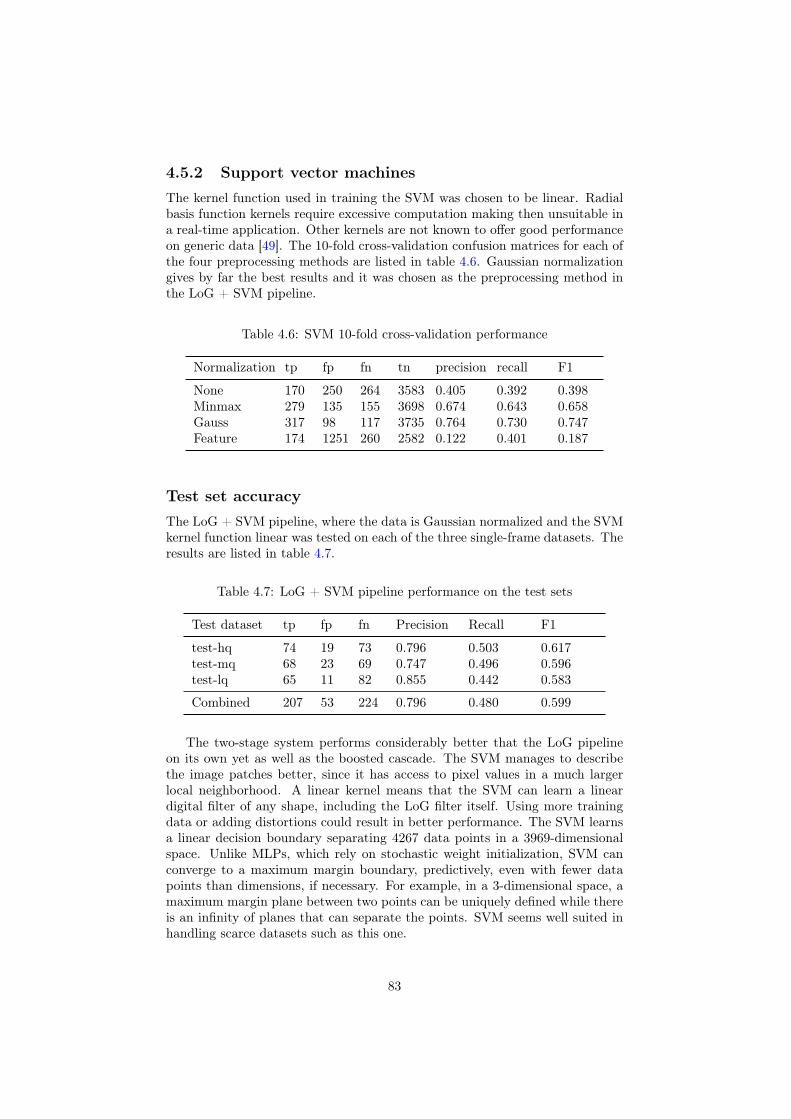
4.5.2 Support vector machinesThe kernel function used in training the SVM was chosen to be linear. Radialbasis function kernels require excessive computation making then unsuitable ina real-time application. Other kernels are not known to offer good performanceon generic data [49]. The 10-fold cross-validation confusion matrices for each ofthe four preprocessing methods are listed in table 4.6. Gaussian normalizationgives by far the best results and it was chosen as the preprocessing method inthe LoG + SVM pipeline.
Table 4.6: SVM 10-fold cross-validation performance
Normalization tp fp fn tn precision recall F1
None 170 250 264 3583 0.405 0.392 0.398Minmax 279 135 155 3698 0.674 0.643 0.658Gauss 317 98 117 3735 0.764 0.730 0.747Feature 174 1251 260 2582 0.122 0.401 0.187
Test set accuracyThe LoG + SVM pipeline, where the data is Gaussian normalized and the SVMkernel function linear was tested on each of the three single-frame datasets. Theresults are listed in table 4.7.
Table 4.7: LoG + SVM pipeline performance on the test sets
Test dataset tp fp fn Precision Recall F1
test-hq 74 19 73 0.796 0.503 0.617test-mq 68 23 69 0.747 0.496 0.596test-lq 65 11 82 0.855 0.442 0.583
Combined 207 53 224 0.796 0.480 0.599
The two-stage system performs considerably better that the LoG pipelineon its own yet as well as the boosted cascade. The SVM manages to describethe image patches better, since it has access to pixel values in a much largerlocal neighborhood. A linear kernel means that the SVM can learn a lineardigital filter of any shape, including the LoG filter itself. Using more trainingdata or adding distortions could result in better performance. The SVM learnsa linear decision boundary separating 4267 data points in a 3969-dimensionalspace. Unlike MLPs, which rely on stochastic weight initialization, SVM canconverge to a maximum margin boundary, predictively, even with fewer datapoints than dimensions, if necessary. For example, in a 3-dimensional space, amaximum margin plane between two points can be uniquely defined while thereis an infinity of planes that can separate the points. SVM seems well suited inhandling scarce datasets such as this one.
83
4.5.3 Effect of compression on performanceIn section 3.1.4 it was established that the size of the video files can be reducedby two orders of magnitude when compressed using the x264 open source H.264encoder. Some of this decrease can be owed to exploiting spatial and temporalstatistical redundancies in the data although most savings are attained by dis-carding information that is deemed irrelevant to the human visual system. Fora scalar quantizer below 28, most of the discarded information is very high fre-quency noise, which would only impede analysis of the video. From 28 onward,lower frequency data is removed, including tag and bee edges. By quantizer 40,visual quality decreases substantially even for a human observer.
The performance of three tag detection systems is analyzed from the effectcompression has on detection F1 measure. To this end, the three single-framedataset were selected, not only to be far apart from the training set in displayorder but mostly for the way they are compressed. The test-hq frame is alwaystreated as an I-frame, the first frame in a chunk of 250 consecutive frames thatis compressed independently of other blocks. Since all frames in this chunk arepredicted based on test-hq, when the video is compressed with a scalar quantizerQPvideo, test-hq is compressed using intra-coded prediction with QPvideo − 3.test-mq is always a P-frame, exactly in the middle of a 250 frame chunk. It isinter-coded based on the preceding P-frame using a quantizer of QPvideo. Forhigh quantizers, the farther away a frame is from the I-frame within a chunk,the poorer its quality, defined by MSE. A P-frame in the middle of the chunkshould approximate well the average quality across the video. test-hq is thelast B-frame in 250 frame chunk. It is inter-predicted from the preceding andsucceeding P-frames with a quantizer of QPvideo + 2 ans show be among theworst quality frames in the video.
Only the tag position information from each of the three dataset was used.For quantizer value QP ∈ {0, 4, ..., 40}, the tag centers were marked on top ofthe compressed versions of the three original dataset frames. When LoG pipelinebased methods were employed, the median over 1 hour of the compressed videowas computed and used in the tests.
All systems were trained once, on the uncompressed version of the train-3dataset. It was expected that the compression would generally result in loweraccuracy metrics as it would alter data in a manner not reflected in the trainingset.
The F1 scores of the original LoG pipeline (threshold 15.85) on the threedatasets, as a function of QPvideo are shown in figure 4.28. In the range [0, 32],QPvideo does not significantly affect the F1 score. The difference between thevideo quantizer and frame quantizer is evident, with the variation on test-hq(I-frame) shifted by almost 4 compared to the other datasets. For a QPvideo of24 (28 in the case of test-hq), the F1 score slightly increases. In this range, noisefrequencies are suppressed, facilitating detection. At this point, the detectionquality is almost the same as when no compression is employed yet the videofile size has been reduced by around 60 times. With higher values of QPvideo,F1 scores decrease steadily for all frames, with a sharp at 40. As mentionedpreviously, QPvalue = 40 results in very low perceived quality, which affects bythe pipeline as well.
The LoG + SVM pipeline, with the SVM having learned a large convolutionkernel for a limited number of samples, shows more erratic fluctuations with
84
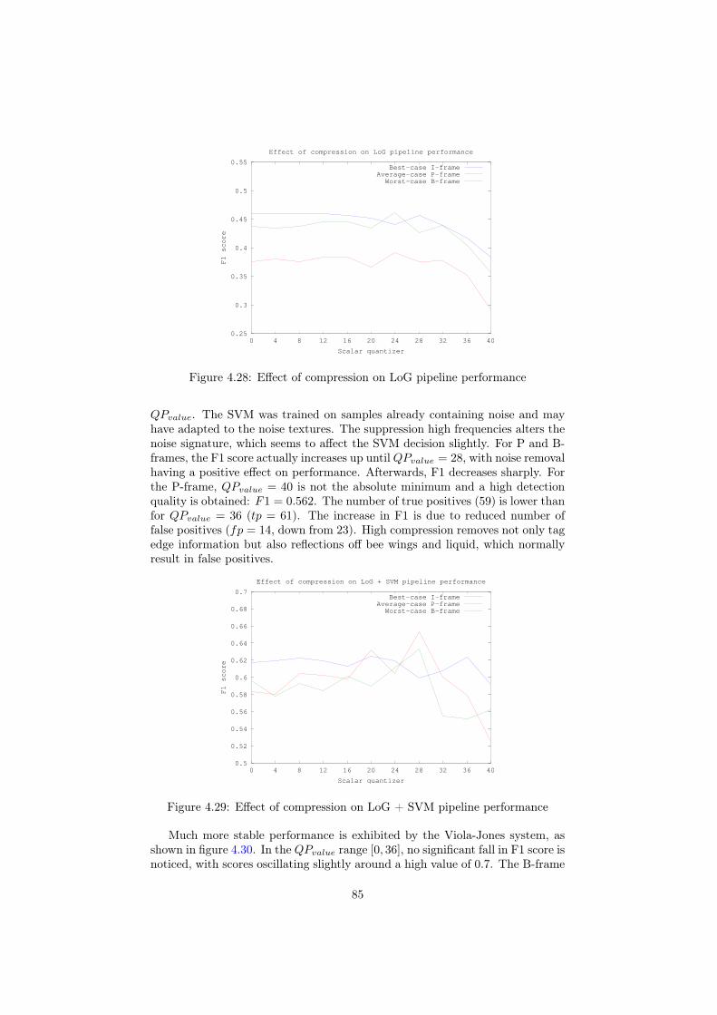
0.25
0.3
0.35
0.4
0.45
0.5
0.55
0 4 8 12 16 20 24 28 32 36 40
F1 score
Scalar quantizer
Effect of compression on LoG pipeline performance
Best-case I-frameAverage-case P-frame
Worst-case B-frame
Figure 4.28: Effect of compression on LoG pipeline performance
QPvalue. The SVM was trained on samples already containing noise and mayhave adapted to the noise textures. The suppression high frequencies alters thenoise signature, which seems to affect the SVM decision slightly. For P and B-frames, the F1 score actually increases up untilQPvalue = 28, with noise removalhaving a positive effect on performance. Afterwards, F1 decreases sharply. Forthe P-frame, QPvalue = 40 is not the absolute minimum and a high detectionquality is obtained: F1 = 0.562. The number of true positives (59) is lower thanfor QPvalue = 36 (tp = 61). The increase in F1 is due to reduced number offalse positives (fp = 14, down from 23). High compression removes not only tagedge information but also reflections off bee wings and liquid, which normallyresult in false positives.
0.5
0.52
0.54
0.56
0.58
0.6
0.62
0.64
0.66
0.68
0.7
0 4 8 12 16 20 24 28 32 36 40
F1 score
Scalar quantizer
Effect of compression on LoG + SVM pipeline performance
Best-case I-frameAverage-case P-frame
Worst-case B-frame
Figure 4.29: Effect of compression on LoG + SVM pipeline performance
Much more stable performance is exhibited by the Viola-Jones system, asshown in figure 4.30. In the QPvalue range [0, 36], no significant fall in F1 score isnoticed, with scores oscillating slightly around a high value of 0.7. The B-frame
85
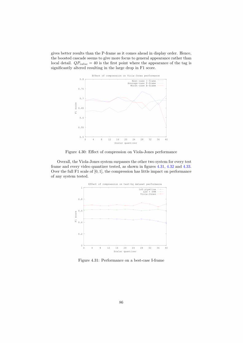
gives better results than the P-frame as it comes ahead in display order. Hence,the boosted cascade seems to give more focus to general appearance rather thanlocal detail. QPvalue = 40 is the first point where the appearance of the tag issignificantly altered resulting in the large drop in F1 score.
0.5
0.55
0.6
0.65
0.7
0.75
0.8
0 4 8 12 16 20 24 28 32 36 40
F1 score
Scalar quantizer
Effect of compression on Viola-Jones performance
Best-case I-frameAverage-case P-frame
Worst-case B-frame
Figure 4.30: Effect of compression on Viola-Jones performance
Overall, the Viola-Jones system surpasses the other two system for every testframe and every video quantizer tested, as shown in figures 4.31, 4.32 and 4.33.Over the full F1 scale of [0, 1], the compression has little impact on performanceof any system tested.
0
0.2
0.4
0.6
0.8
1
0 4 8 12 16 20 24 28 32 36 40
F1 score
Scalar quantizer
Effect of compression on test-hq dataset performance
LoG pipelineLoG + SVM
Viola-Jones
Figure 4.31: Performance on a best-case I-frame
86
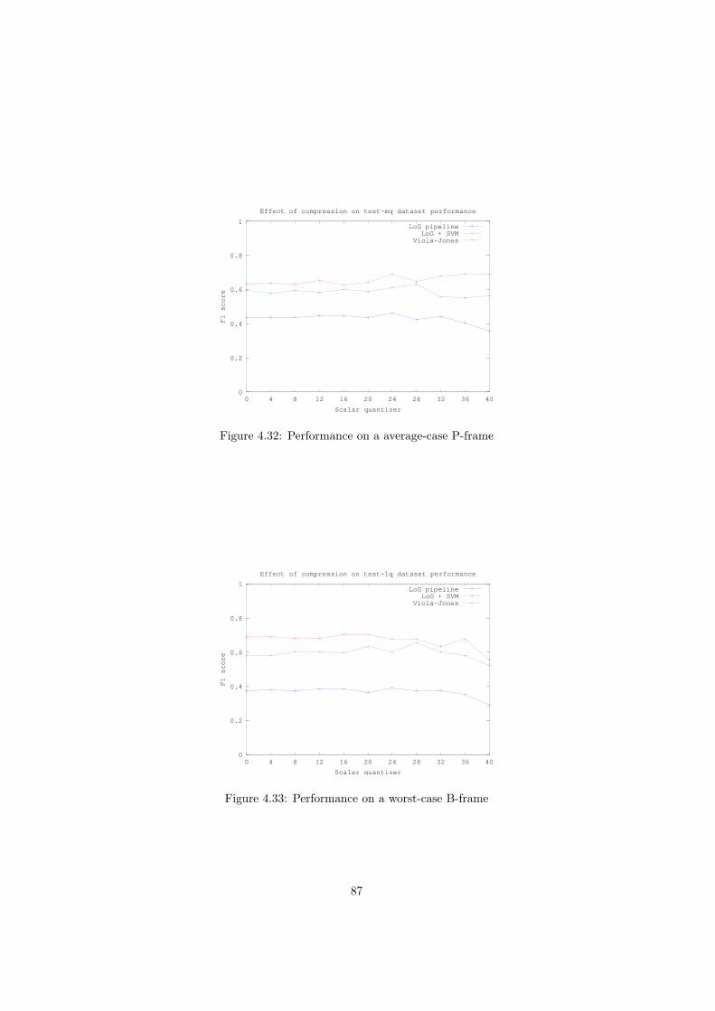
0
0.2
0.4
0.6
0.8
1
0 4 8 12 16 20 24 28 32 36 40
F1 score
Scalar quantizer
Effect of compression on test-mq dataset performance
LoG pipelineLoG + SVM
Viola-Jones
Figure 4.32: Performance on a average-case P-frame
0
0.2
0.4
0.6
0.8
1
0 4 8 12 16 20 24 28 32 36 40
F1 score
Scalar quantizer
Effect of compression on test-lq dataset performance
LoG pipelineLoG + SVM
Viola-Jones
Figure 4.33: Performance on a worst-case B-frame
87
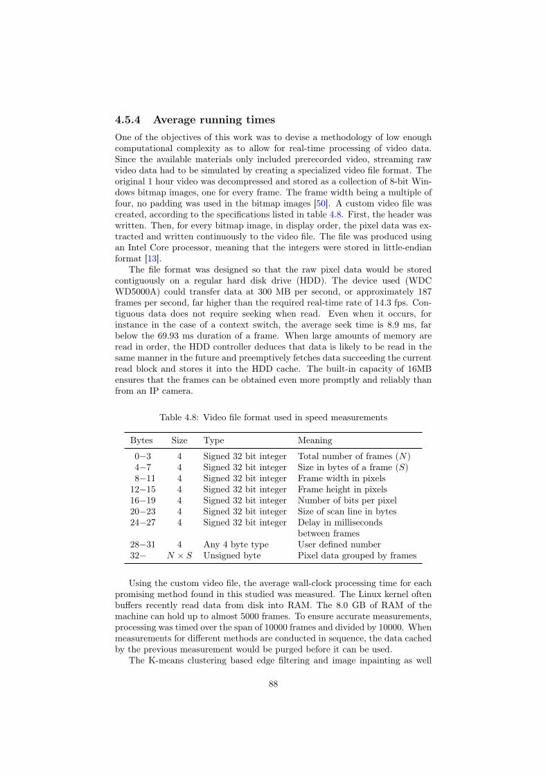
4.5.4 Average running timesOne of the objectives of this work was to devise a methodology of low enoughcomputational complexity as to allow for real-time processing of video data.Since the available materials only included prerecorded video, streaming rawvideo data had to be simulated by creating a specialized video file format. Theoriginal 1 hour video was decompressed and stored as a collection of 8-bit Win-dows bitmap images, one for every frame. The frame width being a multiple offour, no padding was used in the bitmap images [50]. A custom video file wascreated, according to the specifications listed in table 4.8. First, the header waswritten. Then, for every bitmap image, in display order, the pixel data was ex-tracted and written continuously to the video file. The file was produced usingan Intel Core processor, meaning that the integers were stored in little-endianformat [13].
The file format was designed so that the raw pixel data would be storedcontiguously on a regular hard disk drive (HDD). The device used (WDCWD5000A) could transfer data at 300 MB per second, or approximately 187frames per second, far higher than the required real-time rate of 14.3 fps. Con-tiguous data does not require seeking when read. Even when it occurs, forinstance in the case of a context switch, the average seek time is 8.9 ms, farbelow the 69.93 ms duration of a frame. When large amounts of memory areread in order, the HDD controller deduces that data is likely to be read in thesame manner in the future and preemptively fetches data succeeding the currentread block and stores it into the HDD cache. The built-in capacity of 16MBensures that the frames can be obtained even more promptly and reliably thanfrom an IP camera.
Table 4.8: Video file format used in speed measurements
Bytes Size Type Meaning
0−3 4 Signed 32 bit integer Total number of frames (N)4−7 4 Signed 32 bit integer Size in bytes of a frame (S)8−11 4 Signed 32 bit integer Frame width in pixels
12−15 4 Signed 32 bit integer Frame height in pixels16−19 4 Signed 32 bit integer Number of bits per pixel20−23 4 Signed 32 bit integer Size of scan line in bytes24−27 4 Signed 32 bit integer Delay in milliseconds
between frames28−31 4 Any 4 byte type User defined number32− N × S Unsigned byte Pixel data grouped by frames
Using the custom video file, the average wall-clock processing time for eachpromising method found in this studied was measured. The Linux kernel oftenbuffers recently read data from disk into RAM. The 8.0 GB of RAM of themachine can hold up to almost 5000 frames. To ensure accurate measurements,processing was timed over the span of 10000 frames and divided by 10000. Whenmeasurements for different methods are conducted in sequence, the data cachedby the previous measurement would be purged before it can be used.
The K-means clustering based edge filtering and image inpainting as well
88
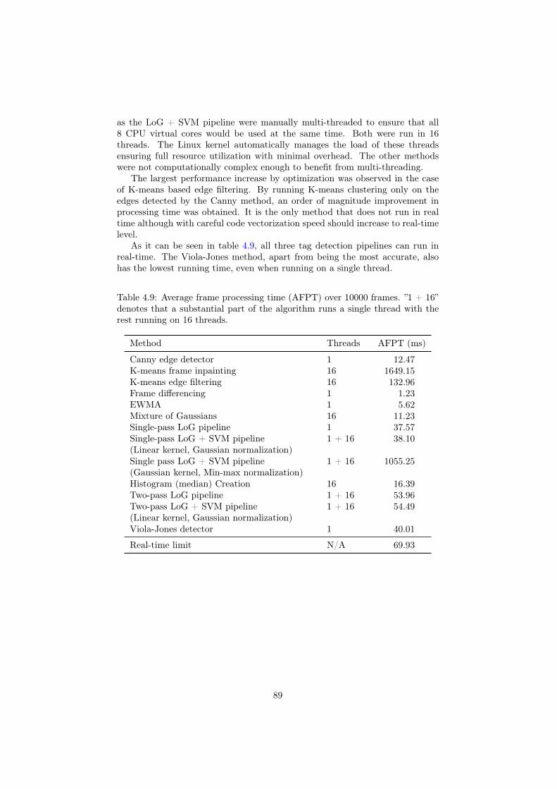
as the LoG + SVM pipeline were manually multi-threaded to ensure that all8 CPU virtual cores would be used at the same time. Both were run in 16threads. The Linux kernel automatically manages the load of these threadsensuring full resource utilization with minimal overhead. The other methodswere not computationally complex enough to benefit from multi-threading.
The largest performance increase by optimization was observed in the caseof K-means based edge filtering. By running K-means clustering only on theedges detected by the Canny method, an order of magnitude improvement inprocessing time was obtained. It is the only method that does not run in realtime although with careful code vectorization speed should increase to real-timelevel.
As it can be seen in table 4.9, all three tag detection pipelines can run inreal-time. The Viola-Jones method, apart from being the most accurate, alsohas the lowest running time, even when running on a single thread.
Table 4.9: Average frame processing time (AFPT) over 10000 frames. ”1 + 16”denotes that a substantial part of the algorithm runs a single thread with therest running on 16 threads.
Method Threads AFPT (ms)
Canny edge detector 1 12.47K-means frame inpainting 16 1649.15K-means edge filtering 16 132.96Frame differencing 1 1.23EWMA 1 5.62Mixture of Gaussians 16 11.23Single-pass LoG pipeline 1 37.57Single-pass LoG + SVM pipeline 1 + 16 38.10(Linear kernel, Gaussian normalization)Single pass LoG + SVM pipeline 1 + 16 1055.25(Gaussian kernel, Min-max normalization)Histogram (median) Creation 16 16.39Two-pass LoG pipeline 1 + 16 53.96Two-pass LoG + SVM pipeline 1 + 16 54.49(Linear kernel, Gaussian normalization)Viola-Jones detector 1 40.01
Real-time limit N/A 69.93
89
Chapter 5
Discussion and future work
5.1 Background removalK-means texture cluster analysis was found ineffective as a preprocessing step fortag detection but it shows promise in filtering foreground edge in order to be fedinto an edge-based antennae detector. If used only for edge filtering, K-meanshas a close to real-time performance as initial experiments have shown. Morework needs to be done on establishing whether K-means is accurate enough toallow for antenna and trophallaxis detection and how an edge-based detectorshould be designed.
Frame differencing worked well at preserving fast moving antennae. A greatdeal of post-processing is required and the exact methodology is left as an openavenue for research. Methods like RANSAC or an adaptive classifier with ori-ented edge features may be viable options.
The median image over 1 hour of video was found to be the best backgroundestimate and it was removed by subtraction. Online techniques would havebeen more desirable although their reliance on learning rate made them imprac-tical. A low learning rate required a very long ”learning” time, wasting largespans of video time while high learning rate resulted in slow moving bees beingassimilated into the background estimate. The mixture of Gaussians methoddid not perform well, partly due to oversimplification of the model to achievecomputational efficiency but mostly due to its reliance on variance in discerningbackground form foreground. Shadows and bees have the same variance andcannot be distinguished by this method. Future work may focus on estimatingseveral background images, such as hive frame and shadows from the temporalhistogram, either by regression or more complex machine learning models.
5.2 Tag detectionThree methods were found to have an adequate tag detection accuracy: a Lapla-cian of Gaussian based pipeline, a cascade made out of a high true positive rateLoG pipeline and Support Vector Machine and the Viola-Jones object detectionframework. The Viola-Jones method had the best performance both in termsof F1 score (0.686) and average computational complexity (40.01 ms per frameon a single thread). The learned cascade had very few features compared to
90
state-of-the-art face detection systems. Training a boosted cascade with thou-sands instead of hundreds of positive samples could further increase accuracy.LoG filter based methods have an upper bound of around 0.9 on recall. Manytags do not resemble the ”Mexican hat” prototype of the LoG filter and cannotbe detected regardless how low a threshold is set. The Viola-Jones method doesnot have recall limitations due to the flexibility of the Haar-like features. It ispossible that, if trained with enough positive samples, the Viola-Jones methodcould reach near-human performance. Tag labeling does not require any techni-cal knowledge and can be undertaken by researchers with basic understandingof the problem.
A problem shared by all tag detection methods was the inconsistency indetection between consecutive frame or ”flickering”. Accuracy can be greatlyimproved by interpolating detection between neighboring frames in display or-der. The particle filters could be used in generating regions in the frame wherebees are likely to move and enforcing detections within that region [51].
The hardware and software barriers pertaining to bee detection in a type Astream have been successfully surmounted. File size was a limiting factor in theamount of video that could be recorded. Using the x264 open source H.264/AVCencoder, the video file size can be reduced by a factor of over 50 with affectingthe performance of any of the tag detection systems employed in this work. Inparticular, the Viola-Jones tag detection system can deliver roughly the sameperformance as on uncompressed data with videos compressed with a scalarquantizer of 36 that are over 360 times smaller in size.
All background removal and tag detection techniques have been shown torequire less than 69 ms of computation per frame, allowing for real time pro-cessing. K-means clustering based edge filtering can be made to run in real-timeas well by writing code optimized for the Intel Core architecture.
A vital factor in obtaining good performance was the utilization of free orotherwise open-source software technology. In particular, the OpenCV opensource computer vision platform has proven to have included implementationsof all basic image analysis techniques employed throughout this work and noother platform was utilized in the experiments. Real-time performance and indepth study of the underlying methods was possible by modifying the sourcecode of some OpenCV primitives. The open nature of the platform allows foradequate reproducible of the experiments carried out in this work, making open-source well suited for academic research.
5.3 Future experimentsEven with advanced detection and tracking methods, whether a tag is validor not is open to interpretation. Manual labeling of positives has proven tobe difficult and a high accuracy was not expected from any system. Recentwork on ant tracking [52] utilized much higher quality materials. The antsmonitored did not rip the tags from their back nor did they walk on top of eachother. The background was made out of a uniform synthetic material and nobackground removal was necessary. Instead of filming at a high framerate withlow resolution, framerate was reduced to around 2 fps, resolution was muchhigher and bursts of light eliminated motion blur and elongated shadows. Mostimportantly, instead of a custom tag design, the well studied ARTags [53] were
91
employed. Well tested detection software was freely available. Several lessonscan be learned from the success of this work. First, it is apparent that detectingtag images 15 × 15 pixels in size is unlikely to be accomplished in a reliablefashion. This work has proven that tag detection is possible at this stage, evenwith high levels of compression. A trade-off can be made by collecting twovideo streams at the same time. One stream (A) can retain the current settings.A second stream (B) can have a higher number of pixels, at least 2 × 2 or3 × 3 times more and be collected with a lower exposure time, a framerate of2 fps and under bursts of infrared light. A camera could be programmed todynamically switch between stream A mode and stream B mode. If this wouldnot be possible, two cameras, one of which can be a programmable still photocamera, can be mounted in close vicinity to have an optical axis as perpendicularto the hive frame as possible. Under these conditions, the frames containingthe lighting bursts can be ignored in stream A. The bursts can also help intemporal alignment of the two streams. If large markings on the corners of thehive frame were to be used, possibly large version of the ARTags themselves,the two streams can be accurately spatially registrated. Stream B would allowfor ARTags to be mounted on the bees. Instead of mounting tags only on thedorsal part of the thorax, pairs of tags could be mounted either on both thedorsal and ventral sized of the thorax or the abdomen as in [7]. The tags canbe detected and identified in stream B. Stream A should only be used in tagdetection. Assuming that very fast motion is unlikely to occur in an 0.5 secondinterval, the information in the two streams can be combined to give an accuratedetection and identification of the bees at 14.3 framerate. Lighting should beimproved overall by using more infrared LED’s and a light diffuser instead ofwide angles, which were found to result in bees casting long shadows.
92
Chapter 6
Conclusions
Using the x264 encoder, file size has been reduced by two orders of magnitudewithout loss of relevant detail. This has been confirmed by the fact that com-pression did not significantly affect the accuracy of any tag detection systemtested.
Almost all methodologies analyzed in this work were implemented to run inreal-time. Year 2013 computing hardware was not found to be a limiting factorin developing a complete real-time bee interaction tracking system.
Viola-Jones object detection framework proved to be the most suitable fordetecting tagged bees. The system delivers high accuracy using only labeleddata, without the need of either formal problem description or encoding of priorknowledge. Better results can be obtained with higher quality video and moretraining samples. The Viola-Jones system is flexible enough to function withother tag designs without the need to write specialized software.
Future filming experiments should employ robust and mature fiducial mark-ers like the ARTags and produce a video stream of higher quality.
93
Acknowledgements
I would like to thank my supervisior Cris Luengo for allowing me to undertakethis degree project in parallel with other courses. Many thanks to Zi Quan Yufor manually tagging the bees and recording the video. My gratitude towardsAnders Brun for proposing K-means clustering as a background removal methodand for his high expectations in the results of this work. Special thanks to OlleTerenius for enthusiastically explaining many apsects of bee society and forgenerously providing the computing hardware on which real-time performancewas attained. Many thanks to Olle Gallmo for our constructive discussions onmachine learning matters. And last, I would like to express esteem towardsprofessor Carlos Adriel Del Carpio at Tohoku Univeristy for painstainkinglyproofreading the manuscript, offering valuable advice on academic writing andespecially for his inspirational guidance on scholarly values.
94

Bibliography
[1] Karl von Frisch. Bees: Their Vision, Chemical Senses, and Language.Cornell University Press, Ithaca, New York, 1963.
[2] Cris Luengo Hendriks, Ziquan Yu, Antoine Lecocq, Teatske Bakker, Bar-bara Locke, and Olle Terenius. Identifying all individuals in a honeybee hive: progress towards mapping all social interactions. In Visual observationand analysis of animal and insect behavior, pages 5–8, 2012.
[3] Aristotle. Historia Animalium Vol. 1, Books I-X. Cambridge UniversityPress, 2002.
[4] Zia Khan, Tucker Balch, and Frank Dellaert. A rao-blackwellized particlefilter for eigentracking. IEEE Computer Vision and Pattern Recognition,pages 980–986, 2004.
[5] Adam Feldman and Tucker Balch. Representing honey bee behavior forrecognition using human trainable models. Adaptive Behavior, 12:241–250,2004.
[6] Antoine Lecocq. The development of tools for network analysis in the honeybee (apis mellifera l.). Master’s thesis, Swedish University of AgriculturalSciences, Faculty of Natural Resources and Agricultural Sciences, Dept. ofEcology, 2011.
[7] A. Meshi and G. Blogh. Monitoring circadian rhythms of individual honeybees in a social environment reveals social influences on post-embryonicontogeny of activity rhythms. Journal of Biological Rhythms, 22(4):343–355, 2007.
[8] R. Okada T. Kimura, M. Ohashi and H. Ikeno. A new approach for thesimultaneous tracking of multiple honeybees for analysis of hive behaviour.Apidologie, 42(5):607–617, 2011.
[9] Richard Stallman. Viewpoint: Why "open source" misses the point of freesoftware. Commun. ACM, 52(6):31–33, June 2009.
[10] Huffyuv. http://neuron2.net/www.math.berkeley.edu/benrg/huffyuv.html. Accessed: 2013-04-07.
[11] Videolan - x264, the best h.264/avc encoder. www.videolan.org/developers/x264.html. Accessed: 2013-06-01.
95
[12] Iain E. Richardson. The H.264 Advanced Video Compression Standard.John Wiley and Sons, Chichester, West Sussex, UK, second edition, 2010.
[13] David A. Patterson and John L. Hennessy. Computer Organization andDesign: The Hardware Software Interface. Morgan Kaufmann, Burlington,MA, USA, fourth edition, 2009.
[14] Mplayer - the movie player. http://www.mplayerhq.hu. Accessed: 2013-04-07.
[15] Digtv : The home of virtual vcr. http://virtualvcr.sourceforge.net.Accessed: 2013-04-07.
[16] D. A. Huffman. A method for the construction of minimum redundancycodes. Proc. IRE, 40(10):1098–1101, 1952.
[17] Eric Hamilton. Jpeg file interchange format - version 1.02. http://www.jpeg.org/public/jfif.pdf, 1992. Accessed: 2013-06-20.
[18] Jason Garrett-Glaser. Diary of an x264 developer. http://x264dev.multimedia.cx/archives/377, 2010. Accessed: 2013-06-20.
[19] John Canny. A computational approach to edge detection. IEEE Trans.Pattern Anal. Mach. Intell., 8(6):679–698, June 1986.
[20] Opencv (open source computer vision). http://opencv.org. Accessed:2013-05-12.
[21] Rafael C. Gonzalez and Richard E. Woods. Digital Image Processing. Pear-son Prentice Hall, Upper Saddle River, NJ, USA, third edition, 2008.
[22] Simon Haykin. Neural Networks and Learning Machines. Person Education,Upper Saddle Rive, NJ, USA, third edition, 2009.
[23] S. P. Lloyd. Least squares quantization in pcm. IEEE Transactions onInformation Theory, 28:129–137, 1982.
[24] Gary Bradski and Adrian Kaehler. Learning OpenCV. O’Reilly Media,Sebastopol, CA, USA, 2008.
[25] G. E. P. Box, G. M. Jenkins, and J. F. MacGregor. Some recent advancesin forecasting and control. Applied Statistics, 23:158–179, 1974.
[26] Milan Sonka, Vaclav Hlavac, and Roger Boyle. Image Processing, Analysis,and Machine Vision. Cengage Learning, Stamford, CT, USA, third edition,2008.
[27] Chris Stauffer and W. E L Grimson. Adaptive background mixture modelsfor real-time tracking. In Computer Vision and Pattern Recognition, 1999.IEEE Computer Society Conference on., volume 2, pages 246–252, 1999.
[28] Georges Voronoi. Nouvelles applications des parametres continus a la the-orie des formes quadratiques. Journal fur die reine und angewandte Math-ematik, 1908:97–102, 1908.
96
[29] Corinna Cortes and Vladimir Vapnik. Machine Learning, volume 20, pages273–297. Kluwer Academic Publishers, Boston, US, 1995.
[30] C. J. van Rijsbergen. Information Retrieval. Butterworths, London, UK,second edition, 1979.
[31] Zi Quan Yu. Tracking individual bees in a beehive. Master’s thesis, De-partment of Information Technology, 2013.
[32] David M. Green and John A. Swets. Signal detection theory and psy-chophysics. John Wiley and Sons Inc., New York, NY, USA, 1966.
[33] Paul Viola and Michael Jones. Robust real-time object detection. In In-ternational Journal of Computer Vision, 2001.
[34] Robert Laganiere. OpenCV 2 Computer Vision Application ProgrammingCookbook. Packt Publishing, Olton, Birmingham, UK, 2011.
[35] Judson P Jones and Larry A Palmer. An evaluation of the two-dimensionalgabor filter model of simple receptive fields in cat striate cortex. Journalof Neurophysiology, 58(6):1233–1258, 1987.
[36] Rainer Lienhart and Jochen Maydt. An extended set of haar-like featuresfor rapid object detection. In IEEE ICIP 2002, pages 900–903, 2002.
[37] Frank Rosenblatt. The perceptron: A probabilistic model for informationstorage and organization in the brain. Psychological Reviews, 65(6):386–408, November 1958.
[38] Robert E. Schapire. Nonlinear Estimation and Classification, chapter TheBoosting Approach to Machine Learning: An Overview. Springer, 2003.
[39] Yoav Freund and Robert E Schapire. A decision-theoretic generalization ofon-line learning and an application to boosting. Journal of Computer andSystem Sciences, 55(1):119–139, 1997.
[40] RobertE. Schapire and Yoram Singer. Improved boosting algorithms usingconfidence-rated predictions. Machine Learning, 37(3):297–336, 1999.
[41] Philip M. Long and Rocco A. Servedio. Random classification noise defeatsall convex potential boosters. In 25th international conference on Machinelearning, pages 608–615, 2008.
[42] Robert E. Schapire, Yoav Freund, Peter Bartlett, and Wee Sun Lee. Boost-ing the margin: A new explanation for the effectiveness of voting methods.The Annals of Statistics, 26(5):1651–1686, 1998.
[43] J.R. Quinlan. Induction of decision trees. Machine Learning, 1(1):81–106,1986.
[44] Yann Lecun and Corinna Cortes. The MNIST database of handwrittendigits. http://yann.lecun.com/exdb/mnist/. Accessed: 2013-05-30.
[45] Andries P. Engelbrecht. Computational Intelligence - An Introduction. JohnWiley and Sons, Chichester, West Sussex, UK, second edition, 2007.
97

[46] David E. Rumelhart, Geoffrey E. Hinton, and Ronald J. Williams. Learningrepresentations by back-propagating errors. Nature, 323:533–536, October1986.
[47] M. Riedmiller and H. Braun. A direct adaptive method for faster backprop-agation learning: the rprop algorithm. In Neural Networks, 1993., IEEEInternational Conference on, pages 586–591 vol.1, 1993.
[48] D. Nguyen and B. Widrow. The truck backer-upper: an example of self-learning in neural networks. In Neural Networks, 1989. IJCNN., Interna-tional Joint Conference on, volume 2, pages 357–363, June 1989.
[49] Chih-Chung Chang and Chih-Jen Lin. LIBSVM: A library for supportvector machines. ACM Transactions on Intelligent Systems and Technology,2:27:1–27:27, 2011. Software available at http://www.csie.ntu.edu.tw/~cjlin/libsvm.
[50] Feng Yuan. Windows Graphics Programming: Win32 GDI and DirectDraw.Hewlett-Packard Professional Books, Upper Saddle River, NJ, USA, 2000.
[51] Olle Gallmo. private communication, 2013.
[52] Danielle P. Mersch, Alessandro Crespi, and Laurent Keller. Tracking indi-viduals shows spatial fidelity is a key regulator of ant social organization.Science, 340(6136):1090–1093, 2013.
[53] M. Fiala. Comparing artag and artoolkit plus fiducial marker systems.In Haptic Audio Visual Environments and their Applications, 2005. IEEEInternational Workshop on, pages 148–153, October 2005.
[54] Ffmpeg. http://ffmpeg.org. Accessed: 2013-04-07.
[55] Libav - open source audio and video processing tools. http://libav.org.Accessed: 2013-04-07.
98
Appendix A
Video transcoding
Because of scarcity of free video recording software on the Microsoft Windowsplatform used by the experimenters, the video has been recorded using VirtualVCR freeware [15]. The only lossless compression method available was thepoorly supported Huffman YUV. Transcoding was complicated by the fact thatvideo has been cropped to a width that is not a multiple of 4. As of 2013,this video frame size is no longer supported by libavcodec, which is currentlyamong the most popular free video transcoding libraries. It is employed byboth FFMpeg [54] and Mencoder [14] software projects. A fork of FFMpeg,called libav [55], contains a modified variant of libavcodec that does not havethis limitation. However, the version libav utilized (9.3 ) had poor containersupport for long video files. Mencoder SVN-r31628-4.4.4 or earlier and FFmpeg0.7.1 or earlier were found suitable. Both are command line applications withextensive manuals.
FFMpeg and, especially, Mencoder were designed to transcode motion pic-tures and television programming and thus offer extensive support for inter-lacing/deintelacing and telecine. Their manuals also focus on encoding videofor the best possible viewing quality and in formats that are popular in theentertainment industry. By contrast, the video utilized in this research projectrequires a constant quality throughout the sequence and was obtained from adigital camera as a series of progressive frames.
Going through the official documentation and extracting relevant commandline options has proven tedious both because of the sheer number of options andof the fact that parts of the documentation were out of date. To those who maywant to employ video transcoding in their research, table A.1 has been whencompiled with ease of use in mind.
99
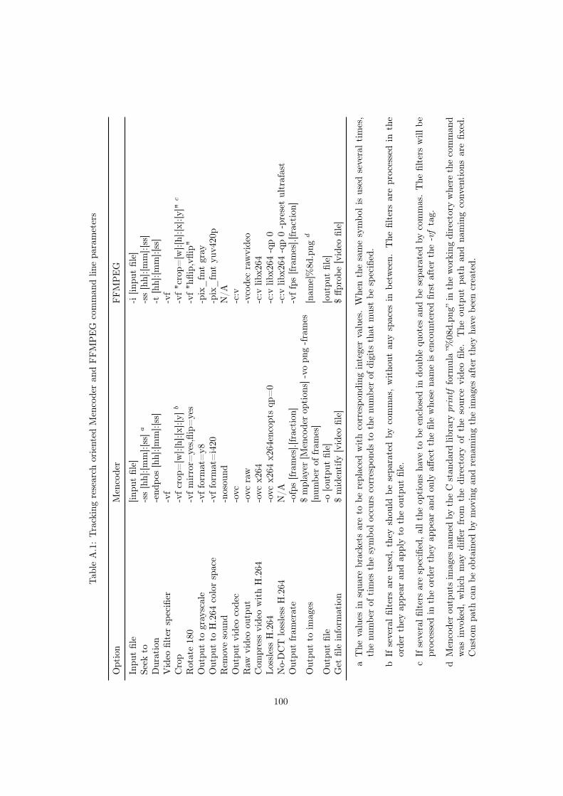
Tab
leA.1:Trackingresearch
oriented
Mencoderan
dFFMPEG
comman
dlin
epa
rameters
Option
Mencoder
FFMPEG
Inpu
tfile
[inpu
tfile]
-i[in
putfile]
Seek
to-ss[hh]:[m
m]:[ss]a
-ss[hh]:[m
m]:[ss]
Duration
-end
pos[hh]:[m
m]:[ss]
-t[hh]:[m
m]:[ss]
Video
filterspecifier
-vf
-vf
Crop
-vfcrop
=[w]:[h]:[x
]:[y]
b-vf"crop=
[w]:[h]:[x
]:[y]"c
Rotate180
-vfmirror=
yes,flip=
yes
-vf"h
flip,vfl
ip"
Outpu
tto
gray
scale
-vfform
at=y8
-pix_fm
tgray
Outpu
tto
H.264
colorspace
-vfform
at=i420
-pix_fm
tyu
v420p
Rem
ovesoun
d-nosou
ndN/A
Outpu
tvideocodec
-ovc
-c:v
Raw
videoou
tput
-ovc
raw
-vcode
crawvideo
Com
pressvideowithH.264
-ovc
x264
-c:v
libx2
64Lo
ssless
H.264
-ovc
x264
x264encoptsqp
=0
-c:v
libx2
64-qp0
No-DCT
lossless
H.264
N/A
-c:v
libx2
64-qp0-presetultrafast
Outpu
tfram
erate
-ofps[fram
es].[fraction
]-vffps[fram
es].[fraction
]
Outpu
tto
images
$mplayer
[Men
coderop
tion
s]-vopn
g-frames
[num
berof
fram
es]
[nam
e]%8d
.png
d
Outpu
tfile
-o[outpu
tfile]
[outpu
tfile]
Get
fileinform
ation
$midentify
[video
file]
$ffp
robe
[video
file]
aThe
values
insqua
rebrackets
areto
bereplaced
withcorrespo
ndingintegervalues.W
henthesamesymbo
lis
used
severaltimes,
thenu
mbe
rof
times
thesymbo
loccurscorrespo
ndsto
thenu
mbe
rof
digits
that
mustbe
specified.
bIf
severalfilters
areused,they
shou
ldbe
sepa
ratedby
commas,witho
utan
yspaces
inbe
tween.
The
filters
areprocessedin
the
orderthey
appe
aran
dap
plyto
theou
tput
file.
cIf
severalfi
ltersarespecified,a
lltheop
tion
sha
veto
beenclosed
indo
uble
quotes
andbe
sepa
ratedby
commas.The
filters
will
beprocessedin
theorderthey
appe
aran
don
lyaff
ectthefilewho
sena
meis
encoun
teredfirst
afterthe-vftag.
dMencoderou
tputsim
ages
named
bytheC
stan
dard
library
printf
form
ula”%
08d.pn
g”in
theworking
directorywhere
thecomman
dwas
invoked,
which
may
diffe
rfrom
thedirectoryof
thesource
videofile.
The
output
path
andna
mingconv
ention
sarefix
ed.
Custom
path
canbe
obtained
bymovingan
drena
mingtheim
ages
afterthey
have
been
created.
100
Appendix B
Improving the custom tagsthrough ID choice
In the videos analyzed in this work, the experiments chose the tag IDs in se-quence, starting from zero to the number of tags. Many tags got lost eitherbecause the bees managed to remove the tags from their back or died and hadto be removed along with the tags. Still the IDs did not go beyond 500. Byimposing constraints on the IDs, their range can be extended and tags that areeasier to be analyzed by an automated system can be produced.
Originally, each of the 8 patches can represent a base 3 digit that is in-dependent from the others. The number of possible IDs encoded this way is38 = 6561. Shadows affect both the brightness and contrast of the tags. Thecenter white dot has the highest possible gray value (255) though there is noguaranteed low value. If the tags were constrained to always contain at east oneblack patch (encoding digit 0), the original tag gray values could be restoredthrough min-max normalization. The number of IDs under these constraints isthe number of IDs without constrains minus the number of ID that do not haveany black patch at all. A non-black patch can only encode 2 possible values(1 or 2) and these total 28 combinations. Thus, the number of patches thatcontain at least a black patch is given by 38 − 28 = 6305. The range reductionsmall compared to the potential benefits.
Let Ntotal = 6561 be the total number of IDs under no constraints. LetNi1,i2,... be the number of IDs that don’t contain digits i1, i2 and so forth.
If the center dot and line would be left out of the min-max normalization,it may be useful to always have at least one 0 patch and one 2 patch. Thetotal number of tags under these constraints is Ntotal − N0 − N2 + N0,2 =38 − 28 − 28 + 18 = 6050.
If gray levels are distorted in a non-linear fashion, it may be necessary tohave at least one of each digits in order to restore the tags by analyzing thehistogram. The number of IDs would be in this case Ntotal −N0 −N1 −N2 +N0,1 + N1,2 + N2,0 − N0,1,2 = 38 − 28 − 28 − 28 + 18 + 18 + 18 − 0 = 5796.Again, even under heavy constraints, the ID range is large enough to easilyaccommodate a whole hive.
If transitions between neighboring patches were detected, detection could besimplified with neighboring patches on either side would encode different digits.
101
Patches on one side need not differ from the other as the center dot and lineare guaranteed in differ in gray levels. Without affecting the result, it can beassumed that the patches in the front left and front right of the tag (the whiteline points towards from front) can take any of the 3 values while all othersare restricted to have only 2 values. The total number of IDs would be thus(3 ·23) ·(3 ·23) = 32 ·26 = 576. This is still enough to encode a small hive and thelimited choice of IDs can be used in error checking. The probability of a decodedID being valid, assuming uniformly random error would be 576
6561 = 8.78%, whichwould perform better than a 3 bit checksum (12.5%).
For larger ID-ranges, the checksum could be embedded in the ID choice withgreater ranges allowing for greater choice.
In general, if k is the base of the digit being encoded in a tag, p the numberof digits, n the number of digits that must occur at least once in each tag, thenthe number of IDs is given by
N = Ntotal −k∑
i1=0
Ni1 +
k∑i1,i2=0,i1 6=i2
Ni1,i2 −k∑
i1,i2,i3=0,i1 6=i2,i16=i3
Ni1,i2,i3 + ... (B.1)
which can be expressed in terms of combinations Cqn = n!q!·(n−q)! as:
N =
k∑q=0
(−1)q · Cqn · (k − q)p (B.2)
102