autonomous fire detection robot using modified voting … · autonomous fire detection robot using...

1

Autonomous Fire Detection Robot Using

Modified Voting Logic

by

Adeel ur Rehman

Thesis submitted to the Faculty of Graduate and Postdoctoral Studies

In partial fulfillment of the requirements For the Master’s in Applied Science degree in

Mechanical Engineering

Department of Mechanical Engineering Faculty of Engineering University of Ottawa

© Adeel ur Rehman, Ottawa, Canada, 2015

2

Abstract:

Recent developments at Fukushima Nuclear Power Plant in Japan have created

urgency in the scientist community to come up with solutions for hostile industrial

environment in case of a breakdown or natural disaster.

There are many hazardous scenarios in an indoor industrial environment such as

risk of fire, failure of high speed rotary machines, chemical leaks, etc. Fire is one of the

leading causes for workplace injuries and fatalities[1]. The current fire protection systems

available in the market mainly consist of a sprinkler systems and personnel on duty. In

the case of a sprinkler system there could be several things that could go wrong, such as

spraying water on a fire created by an oil leak may even spread it, the water from the

sprinkler system may harm the machinery in use that is not under the fire threat and the

water could potentially destroy expensive raw material, finished goods and valuable

electronic and printed data.

There is a dire need of an inexpensive autonomous system that can detect and

approach the source of these hazardous scenarios. This thesis focuses mainly on

industrial fires but, using same or similar techniques on different sensors, may allow it to

detect and approach other hostile situations in industrial workplace.

Autonomous robots can be equipped to detect potential threats of fire and find out

the source while avoiding the obstacles during navigation. The proposed system uses

Modified Voting Logic Fusion to approach and declare a potential fire source

autonomously. The robot follows the increasing gradient of light and heat intensity to

identify the threat and approach the source.

3

Dedication This thesis is dedicated to my parents without whose prayers I would not have been able

to finish this work, and to Faiqa, whose love, encouragement and support helped me in

this journey of mine, and last but not least to Muawiz, Zahra and Zainab whose innocent

questions, suggestions, words of encouragement and prayers opened so many doors for

me.

4

Acknowledgements I would like to express my gratitude to my supervisor Dr. Dan Necsulescu whose

continuous guidance, encouragement and support made it possible for me to finish this

work, and to Dr. Jurek Sasiadek whose reviews and inputs helped me improve different

aspects of this thesis.

I would also like to thank (late) Dr. Atef Fahim who saw the capability in me the first

time and took me under his supervision.

Also I would like to express my thanks to my colleagues in the lab whose ideas, help and

support played a big part in the completion of this thesis.

Most importantly I would like to thank the Creator who made everything possible for me

to achieve and gave me strength, courage and guidance to go through this phase of my

life.

5

Table of Contents Abstract: .......................................................................................................................... 2

Dedication ................................................................................................................... 3

Acknowledgements ..................................................................................................... 4

Table of Contents ........................................................................................................ 5

List of Figures ............................................................................................................. 7

List of Tables ............................................................................................................ 10

Chapter 1 Introduction ........................................................................................... 11

1.1 Motivation: ..................................................................................................... 11

1.2 Research Objective: ........................................................................................ 13

1.3 Method of Approach ....................................................................................... 14

1.4 Thesis Outline: ................................................................................................ 15

Chapter 2 Literature Review ................................................................................. 17

Chapter 3 The Robot NXT 2.0 ............................................................................... 22

3.1 Programmable 32-bit Brick ............................................................................ 23

3.2 Inputs for Mindstorms ™ ............................................................................... 24

3.3 Outputs for Mindstorms ™ ............................................................................. 27

3.4 The Assembly: ................................................................................................... 28

3.5 Robot Operation: ............................................................................................ 30

3.6 Robot Kinematics ........................................................................................... 32

Chapter 4 Gradient Increase Approach .................................................................... 35

Relationship between distance from the light source and light intensity .................. 35

Chapter 5 Navigation Strategy ................................................................................ 38

5.1 Sinusoidal or Zigzag Movement of the Robot ................................................ 41

5.2 Tracking of a heat source with one sensor ..................................................... 45

5.3 Tracking of the source with TWO sensors ..................................................... 51

5.4 Obstacle Avoidance ........................................................................................ 55

Chapter 6 Voting Logic Fusion.............................................................................. 59

6.1 Introduction .................................................................................................... 59

6.2 Confidence Levels .......................................................................................... 62

6.3 Detection Modes ............................................................................................. 64

6.4 Detection Probability ...................................................................................... 69

Chapter 7 Modified Voting Logic Fusion ............................................................... 74

7.1 Introduction: .................................................................................................. 74

6

7.2 Single Sensor Detection Modes ...................................................................... 74

7.3 Two-sensor Detection and Non-Possibility Modes ........................................ 86

Chapter 8 LabVIEW Program ............................................................................... 97

8.1 Sinusoidal or Zigzag Movement ..................................................................... 98

8.2 Obstacle Avoidance ...................................................................................... 101

8.3 Fire Detection and Approach ........................................................................ 104

8.4 Fire Declaration ............................................................................................ 106

Chapter 9 Experimental Results........................................................................... 120

9.1 Introduction ................................................................................................. 120

9.2 The Target .................................................................................................... 121

9.3 Testing Scenarios ......................................................................................... 122

9.4 Sensor arrangement with two light and one temperature sensor: ................. 122

9.5 Sensor arrangement with one light and two temperature sensors: ............... 149

9.6 Discussion Regarding Experimental Results ................................................ 167

9.7 Conclusions .................................................................................................. 169

9.8 Future Work:................................................................................................. 171

References: .................................................................................................................. 173

7

List of Figures Figure 3. 1 Programmable NXT Brick ......................................................................... 23

Figure 3. 2 Dexter Industries Thermal Infrared Sensor ................................................. 24

Figure 3. 3 Ultrasonic Sensor for Mindstorms® NXT .................................................. 25

Figure 3. 4 Color Sensor for Mindstorms ® NXT ........................................................ 26

Figure 3. 5 Servo Motor with Built-in Rotation Sensor ................................................ 27

Figure 3. 6 The assembled NXT 2.0 with one TIR, two light and color sensors and one ultrasonic sensor.......................................................................................... 29

Figure 3. 7 The Model of a Differentially Driven Two Wheeled Autonomous Robot in a two-dimensional workspace. .................................................................... 32

Figure 4. 1 Light intensity decrease with distance. (NASA Imagine website

http://imagine.gsfc.nasa.gov/YBA/M31-velocity/1overR2-more.html) ..... 35

Figure 5. 1 Sensor Peripheral Vision............................................................................. 40

Figure 5. 2 Sinusoidal movement of the robot and scannable angles ........................... 41

Figure 5. 3 Scannable area and zigzag motion pattern .................................................. 42

Figure 5. 5 LabVIEW Virtual Instrument (VI) for sinusoidal movement of the robot ending as higher levels of light are reached ...................................................................... 43

Figure 5. 6 Flow chart for the zigzag movement of robot ............................................. 44

Figure 5. 7 LabVIEW programming for a while loop with shift register showing the true case of increasing gradient of object temperature ..................................................... 47

Figure 5. 8 LabVIEW programming for a while loop with shift register showing false case for increasing gradient of object temperature ........................................................... 48

Figure 5. 9 Block diagram for one sensor gradient increase VI ................................... 49

Figure 5. 10 Temperature waveform for the single sensor based increasing gradient trail guidance 50

Figure 5. 11 Two light-sensor tracking system .......................................................... 52

Figure 5. 12 VI for two sensor source approaching..................................................... 53

Figure 5. 13 Block diagram for two-sensor light following ........................................ 54

Figure 5. 14 Front Panel for two-sensor light tracking system.................................... 54

Figure 5. 15 Intelligent obstacle avoidance keeping into account the direction of backing up 56

Figure 5. 16 Block diagram for obstacle avoidance ................................................... 56

Figure 5. 17 Obstacle Avoidance................................................................................ 57

Figure 5. 18 Front panel results for obstacle avoidance with record of temperature readings 58

8 Figure 6. 1 Parallel sensor arrangement [17] ................................................................ 60

Figure 6. 2 Venn diagram for parallel sensor arrangement [17] ................................... 60

Figure 6. 3 Series sensor arrangement with Venn diagram[17] ................................... 60

Figure 6. 4 Series/Parallel configuration of sensor arrangement [17] ........................... 61

Figure 7. 1 Possible combinations of sensor readings................................................... 76

Figure 7. 2 Fire present at First detection mode A1 ....................................................... 77

Figure 7. 3 Fire present at First detection mode A2B2 ................................................... 77

Figure 7. 4 Fire present at First detection mode A2C2 .................................................. 78

Figure 7. 5 Fire present at First detection mode A3B1C2 .............................................. 78

Figure 7. 6 Fire present at First detection mode A3B2C1 .............................................. 79

Figure 7. 7 Possible combinations of sensors with A and B as heat sensors and C as a light sensor 87

Figure 8. 1 Movement control of the robot before elevated heat or light has been

detected ..................................................................................................... 100

Figure 8. 2 Case structure showing even values at label “H” ..................................... 100

Figure 8. 3 Block diagram for zigzag movement ........................................................ 100

Figure 8. 4 No actions taken while the obstacle is more than 25 cm away ................ 102

Figure 8. 5 Obstacle Avoidance with light intensity comparison ............................ 102

Figure 8. 6 Block diagram for smart obstacle avoidance ............................................ 103

Figure 8. 7 Light following program while light sensor connected to Port 1 has a higher value than the one connected to Port 2 (Robot turns right) ........... 105

Figure 8. 8 Light trail following while light sensor connected to Port 2 has a higher value than the one connected to port 1 (Robot turns left) ......................... 105

Figure 8. 9 Sensors and confidence levels .................................................................. 108

Figure 8. 10 Detection Modes in accordance to Eq. 7.1 ................................................ 111

Figure 8. 11 The actual detection VI for this sensor arrangement............................. 113

Figure 8. 12 Confidence level definition for the case of two TIR sensors and one light sensor ...................................................................................................... 114

Figure 8. 13 Detection Modes for two TIR and one Light sensor arrangement in accordance to eq. 7.7 ............................................................................... 115

Figure 8. 14 Open loop control of Motor A is running indicating the true condition of the presence of fire .................................................................................. 116

Figure 8. 15 Open loop control of Motor A is stopped indicating the false condition of the presence of fire .................................................................................. 116

Figure 8. 16 Complete LabVIEW VI for Fire Declaration algorithm with two light and one TIR sensors. Describing Eq. 7.4....................................................... 119

Figure 8. 17 Complete LabVIEW VI for Fire Declaration algorithm with one light and two TIR sensors in accordance with Eq. 7.7 (The other parts remain the same as figure 8.16 ........................................................................................................... 119

Figure 9. 1 Thermal Infrared light bulb used as fire source ........................................ 121

Figure 9. 2 Robot approach GUI values with no obstacle........................................... 123

Figure 9. 3 Sinusoidal movement of the robot ............................................................. 123

Figure 9. 4 Robot detected elevated light and navigating towards it .......................... 124

9 Figure 9. 5 Robot approaching the target .................................................................... 124

Figure 9. 6 Sensor readings are high but the target is not declared yet ....................... 125

Figure 9. 7 Target declaration using modified voting logic ........................................ 125

Figure 9. 8 Target behind a flat obstacle ..................................................................... 127

Figure 9. 9 Initial approach behind a flat obstacle ...................................................... 128

Figure 9. 10 Sinusoidal movement because of low light values................................ 128

Figure 9. 11 Going around the obstacle ..................................................................... 129

Figure 9. 12 Clearing the obstacle ............................................................................. 129

Figure 9. 13 Target approach ..................................................................................... 130

Figure 9. 14 Target (Source) declaration with detection mode A2B2 ........................ 130

Figure 9. 15 Target present behind a concave obstacle ............................................. 131

Figure 9. 16 Concave obstacle target detected with detection mode A1 ................... 132

Figure 9. 17 Target behind a convex obstacle ........................................................... 133

Figure 9. 18 Target declaration behind a convex obstacle with two detection modes 134

Figure 9. 19 Another case with different detection mode for target present behind a convex obstacle 135

Figure 9. 20 Flat obstacle with a reflective wall ........................................................ 136

Figure 9. 21 Robot follows the reflected light from the obstacle .............................. 137

Figure 9. 22 Robot approaches the reflected light from the obstacle ........................ 137

Figure 9. 23 Robot detects higher values of light and temperature as it turns back facing towards a higher value of light ............................................................................. 138

Figure 9. 24 Robot clears the obstacle and is following the correct source .............. 138

Figure 9. 25 : Source (Target) confirmation be modified voting logic ..................... 139

Figure 9. 26 An explanation of the thermal readings and milestones ....................... 140

Figure 9. 27 Target behind an obstacle with a reflective wall on the side Case 1 ..... 141

Figure 9. 28 Target declaration for same sensor and obstacle arrangement – Case 2 141

Figure 9. 29 Target present behind an obstacle with a non-reflecting wall on the side 142

Figure 9. 30 Sinusoidal or Zigzag movement of the robot because of lower light values 143

Figure 9. 31 Robot turns around to avoid obstacle .................................................... 143

Figure 9. 32 Robot follows visible brightest point .................................................... 144

Figure 9. 33 Robot detects most powerful light signal .............................................. 144

Figure 9. 34 Robot avoids obstacle............................................................................ 145

Figure 9. 35 Robot compares available light values from reflected and light from the source 145

Figure 9. 36 Robot declares fire incident................................................................... 146

Figure 9. 37 Robot navigation with no target present ............................................... 148

Figure 9. 38 LabVIEW VI for two temperature sensors and one light sensor .......... 149

Figure 9. 39 Open loop control for sinusoidal or zigzag movement before the elevated light or temperatures are detected ................................................................................... 150

Figure 9. 40 Comparison of the average of previous four values to the current values collected by the sensor using a while loop with shift register. Case 1............................ 152

Figure 9. 41 Comparison of the average of previous four values to the current values collected by the sensor using a while loop with shift register. Case 2.... 153

10 Figure 9. 42 Block diagram for an increasing gradient following VI corresponding to

Figure 9.41 and 9.42 ............................................................................... 154

Figure 9. 43 Robot declaring a target in plain sight .................................................. 155

Figure 9. 44 Light sensor based navigation approach to the source .......................... 156

Figure 9. 45 Light sensor based declaration .............................................................. 157

Figure 9. 46 Target behind a concave obstacle.......................................................... 158

Figure 9. 47 Target behind a convex obstacle ........................................................... 160

Figure 9. 48 Target behind a flat obstacle with reflective wall on the side ............... 162

Figure 9. 49 Target present behind a flat obstacle with a non-reflective wall on one side 164

Figure 9. 50 No target present scenario ..................................................................... 166

List of Tables Table 4. 1 Relationship of light intensity with distance from the source ..................... 37

Table 6. 2 Some representative features and other attributes of different types of

targets [18] .................................................................................................. 63

Table 6. 3 Three sensor combinations when all sensors inputs are obtained.............. 66

Table 6. 4 Two sensor combinations for sensors A and B ........................................... 67

Table 6. 5 Two sensor combinations for sensors A and C ........................................... 67

Table 6. 6 Two sensor combinations for sensors B and C ........................................... 68

Table 6. 7 Confidence levels in a three-sensor system declaring detection modes ..... 69

Table 7. 1 Distribution of detections among sensor confidence levels ........................ 84

Table 7. 2 Inherent detection probabilities among sensor confidence level ................ 84

Table 7. 3 Inherent false alarm probability for sensor A for all four confidence ........... levels ........................................................................................................... 85

Table 7. 4 Inherent false alarm probabilities for sensors B and C ............................... 85

Table 7. 5 Conditional probabilities for sensors A, B and C in the current combination of the sensors............................................................................................... 94

Table 7. 6 Inherent detection probabilities of the sensors A, B and C obtained as a result of distribution of detections .............................................................. 95

Table 7. 7 Inherent false alarm probabilities for sensor A at different confidence ......... levels ........................................................................................................... 96

Table 7. 8 Inherent false alarm probabilities for sensor B at different confidence ......... levels ........................................................................................................... 96

Table 7. 9 Inherent false alarm probabilities for sensor C at different confidence ......... levels ........................................................................................................... 97

11

Chapter 1

Introduction

1.1 Motivation:

An industrial environment is full of hazards for the workers. There are safety and

security system guidelines in place but there is always room for improvement. After the

Fukushima Nuclear Power Plant disaster in Japan the need of monitoring whole industrial

environment has caught the attention of researchers around the world. These hazards may

be chemical leak, machinery breakdown causing dangerous situations or industrial fire.

Industrial fires are a leading cause of workplace injuries and fatalities. According to

NFPA (National Fire Protection Agency, USA) 2012 statistics, [1]

• 1,375,000 fires were reported in the U.S during 2012.

• 2,855 civilian fire deaths

• One civilian death occurred every 3 hours and 4 minutes

• 16,500 civilian fire injuries

• One civilian injury occurred every 32 minutes

• $12.4billion in property damage

• A fire department responded to a fire every 23 seconds

• 480,500 of these fires were structure fires.

Fire is an abrupt exothermic oxidation of materials that generates light, heat, gases

and some other by-products. If in control, fire is very helpful to humans but if not

contained, in some cases it can be disastrous. [2] The best way to not arrive to a

12 threatening situation is to detect unwanted fire in its early stages and extinguish it before

it spreads to other combustible objects nearby.

This work is particularly important in the case of having a monitoring done at night or

days where active surveillance cannot be performed by a human.

There is a need of an autonomous robot that can detect potential threats of fire in a

workshop and approach the source autonomously while avoiding the obstacles during

navigation.

There are security systems in place in factories that keep the workers safe, for

example, in case of fire, a sprinkler system will be activated helping to contain fires.

However, a sprinkler system may make a larger area wet which could not only be

harmful for the machines but also sometimes that could cause a loss of millions of dollars

by destroying raw materials or finished goods that should not be exposed to water. In

case of a sensitive office building, it may destroy valuable data stored in the computers.

Also some industrial fires actually grow more or are not affected by the use of water as

oil being lighter than water will still burn after thrown water on.

The most efficient way to put out a fire will be using a fire extinguisher at the

source of fire not the whole workshop, after the fire source is declared using an

autonomous fire detection robot. This will also ensure that the production or the work is

not stopped in the whole organization and the areas not under threat of fire are

undisturbed.

13

1.2 Research Objective:

In order to increase the productivity of the currently available options, a robot will

need to scan an area of interest, detect and approach the source of fire accurately and

consistently while avoiding the obstacles autonomously. This robot should have very few

false negatives and false positives, i.e., declaration of a fire when no fire is present and

non declaration of fire where a fire is present. Also this robot should be able to

distinguish between a less likely and a more likely source of fire and prioritize its

investigation.

Certain scenarios will need to be tested and the approach will be refined by using

the mathematical expressions and experimental results.

There are three main scenarios that will be tested.

1. Fire in plain sight of the robot,

2. Fire incident behind an opaque wall and a reflective wall in front reflecting only

the light,

3. Fire incident behind an opaque wall and a non reflective wall present close to the

opening.

14

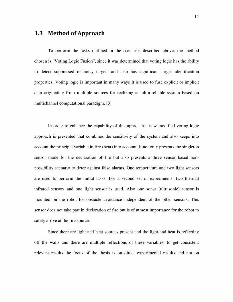
1.3 Method of Approach

To perform the tasks outlined in the scenarios described above, the method

chosen is “Voting Logic Fusion”, since it was determined that voting logic has the ability

to detect suppressed or noisy targets and also has significant target identification

properties. Voting logic is important in many ways It is used to fuse explicit or implicit

data originating from multiple sources for realizing an ultra-reliable system based on

multichannel computational paradigm. [3]

In order to enhance the capability of this approach a new modified voting logic

approach is presented that combines the sensitivity of the system and also keeps into

account the principal variable in fire (heat) into account. It not only presents the singleton

sensor mode for the declaration of fire but also presents a three sensor based non-

possibility scenario to deter against false alarms. One temperature and two light sensors

are used to perform the initial tasks. For a second set of experiments, two thermal

infrared sensors and one light sensor is used. Also one sonar (ultrasonic) sensor is

mounted on the robot for obstacle avoidance independent of the other sensors. This

sensor does not take part in declaration of fire but is of utmost importance for the robot to

safely arrive at the fire source.

Since there are light and heat sources present and the light and heat is reflecting

off the walls and there are multiple reflections of these variables, to get consistent

relevant results the focus of the thesis is on direct experimental results and not on

15 simulation, as each scenario is environment specific and cannot represent another

possible case of fire detection.

1.4 Thesis Outline:

This thesis consists of 9 chapters that walk the reader through different stages of

work.

Chapter 2 provides a literature review of previously published research from

scientists working on similar technology around the world. It also discusses the

advantages and limitations of such work.

Chapter 3 presents the robot used, the reason for this choice, the advantages,

qualities, limitations and challenges of using it. It also describes the kinematics of the

robot.

Chapter 4 discusses the properties of light and heat and how the strength of

signals varies at different distances and includes relevant graphical representations.

Chapter 5 describes the navigation strategy of the robot and presents the

advantages of using the sinusoidal motion approach. It also includes the “VI” or Virtual

Instrument, (another name of LabVIEW programs) designed to achieve this motion

pattern.

Chapter 6 introduces the “Voting Logic” approach and explains the different parts

of it such as confidence levels, sensor fusion, block diagrams and prepares the reader to

understand the approach considering the robot available.

16

Chapter 7 explains the “Modified Voting Logic”, its implementation, confidence

level calculations, detection modes, fire declaration algorithm, its derivation and

explanation. It also presents the calculations of probabilities of detection and false alarms.

Chapter 8 details the experimental results and also discusses certain scenarios. It

also includes the commentary for using different sensor arrangements and modifications

of the hardware where necessary

Finally, Chapter 9 concludes the thesis by discussing the results, conclusions

drawn and providing recommendations for further research.

17

Chapter 2

Literature Review

In their paper, Oleh Adamiv et al. [4] have suggested a regular iterative method of

gradient search based on the local estimation of second order limits. They suggest this

improved method of robot local navigation based on the use of potential fields for

movement taking into account the gradient of direction to the goal. They discuss the

environment for Autonomous Mobile Robot (AMR). In their research, they take into

account that the robot follows the artificial potential fields and has enough clearance from

the obstacles to perform manoeuvres safely. The direction of movement is chosen from

alternative solutions where the value of cost function is largest. In order to determine the

optimal movement path with any influence of AMR of two or more obstacles, the sum of

the cost function values is used based on least-squares method. The navigation of AMR

consists of two stages in this paper, namely the movement to the goal using gradient of

direction to the goal and the value of cost function of obstacles, and obstacle avoidance

along perimeter.

Hu Huosheng, et al. [5] in their paper “Sensors and Data Fusion Algorithms in

Mobile Robotics” have provided a broad overview and understanding of sensor

technologies and data fusion algorithms that have been developed in robotics in general

and mobile robots in particular, with a scope for envisaging their important role in UK

robotics research and development over the next 10 years. The key theme of this report is

to present a brief review on sensor technology. It includes a brief description of the

current advancement of a range of sensors and data fusion algorithms and the reason why

18 it is so hard. Then, a brief summary on sensor and data fusion algorithm development in

the UK is presented, including its position in the world.

E. Zervas et al in the paper “Multisensor data fusion for fire detection” [6], 2008, discuss

the forest fire detection by using the fire detection method constituting of fusion of

temperature, humidity and vision sensors. Each sensor reading is transmitted to a

centralized control unit. A belief of fire probability is established for each resultant node,

and then this data is fused with the vision sensors that monitor the same geographical

area. In the first level the data is fused but in the second stage, the information is also

fused to establish a confidence level of possibility of fire. The first level data fusion

consists of gathering the required data from in-field and out-field sensors. It then goes

through the process of recognition of smoke or flame or in case of in-field sensors it

looks for changes in distribution of data. If there is a detection and distribution change is

detected then the second level (Information Fusion) comes into effect where collection of

probabilities, fusion of probabilities and reasoning about the fire is established.

In the paper "Autonomous Fire Fighting Mobile platform", Teh Nam Khoon[7], et al.

have come up with a novel design of an autonomous robot. This robot, as called by them,

Autonomous Fire Fighting Mobile Platform or AFFPM, has flame sensor and obstacle

avoidance systems. The AFFPM follows a preset path through the building and uses a

guide rail or markers such as black painted line or a tape to navigate through the

environment until it detects an elevated chance of a fire being present. At that point it will

leave its track and follow the fire reaching within 30 cm of the flame. It then would

engage the fire extinguisher that is mounted on the platform. Once it has left the

19 navigation route, the obstacle avoidance will start to perform and it will be able to guide

the AFFPM precisely closer to the source of the fire. When it has extinguished the fire

completely it would then return to its guiding track to carry on with its further

investigation of any other fire sources.

Flame detection in the AFFPM has its limitations as it can only scan the area in front of

the flame detection sensor. Typically the angle of vision of such sensor is 45º. If,

however the robot is programmed to make a 360º turn every now and then, it would

increase the area of vision of the robot, slowing down the robot significantly. Also it

would be using more area for navigation as the track has to have paths circling in a 360˚

in every new room it enters on its way. Typically this robot would go into each room of

the establishment, after a set period of time and perform the required actions, such as

scanning for and extinguishing the fire.

In the paper, “Distributed Detection With Multiple Sensors: Part I—Fundamentals”[8],

Ramnayayan Wiswanath and Pramod K. Varshney discuss some basic results on

distributed detection. They have discussed series and parallel architectures and the

governing decision rules that may be implemented. They also talked about optimization

based on Neyman-Pearson criterion and Bayes formulation for conditionally independent

sensor observations. The optimality of the likelihood ratio test (LRT) at the sensors is

established. General comments on several important issues are made including the

computational complexity of obtaining the optimal solutions, the design of detection

networks with more general topologies, and applications to different areas.

20 In the paper “Cooperative Detection of Moving Targets in Wireless Sensor Network

Based on Fuzzy Dynamic Weighted Majority Voting Decision Fusion” Ahmad Aljaafreh,

and Liang Dong[9] discus the advantages of weighted majority voting decision making to

detect targets.

In another Voting Logic approach, A Boolean Algebra Approach to Multiple Sensor

Voting Fusion, Lawrence A. Klein [10] introduced an algorithm to solve the maze that

avoids the long process to save time and memory. The proposed algorithm is based on

image of the maze and the algorithm works efficiently because of the pre-processing on

the entire maze`s image data before the robot starts navigation, so the robot will have

information about the maze and all the paths; only capturing the image and processing it

will be enough to make the robot navigate to the target without searching because the

path will be known and this will give the robot preplanning time and selection of the

method before falling in mistakes like loops and being trapped in a local minimum. In

this research an algorithm to solve maze discovery problem has been produced, based on

an image of the maze, to create and pre-processing the data of the entire maze. This

avoids the robot traversing long pathways and saves time and memory. Even if it fails to

cover the entire maze it still better then navigating the whole maze cell by cell. Results

show that not all walls are detected properly and this means that image processing

techniques go to approximate half of the maze. For complete solution it doesn't give

proper results, so it is better if it is done in process as long as the robot approaches to the

end and tries to capture more images so it gets more accurate results. Image processing

21 does not give the complete solution; if the image would have been taken from the top of

the maze this would work better, but in this situation it’s not completely appropriate.

D. Necsulescu and Adeel ur Rehman [11] have discussed the “Modified Voting Logic”,

different sensor arrangements and some experimental results claiming that modified

voting logic for target declaration is a valuable technique to identify industrial fires in an

indoor environment. This thesis is based on that paper.

The above works have great contribution to the field but there is a possibility of using

another more productive way of detection and declaration of industrial fires using a

modified voting logic fusion, the approach chosen for investigation in this thesis.

22

Chapter 3

The Robot NXT 2.0 The robot used for these experiments is a non holonomic differentially driven robot

called Mindstorms NXT ®. This light weight easy to assemble robot was chosen due to

the following qualities:

• Lightweight

• Inexpensive

• Easy to build

• Can be programmed in LabVIEW

• Quite accurate and precise

• Is capable of quick changes in the hardware as required by the user

• Is compatible with a number of sensors including light, color, proximity, touch,

PIR, TIR, gyroscope and other sensors.

Some of the limitations include

• Only four inputs can be connected at one time

• Very low profile on the ground

• Slow

• Does not have support for smoke sensors

The robot can be constructed in accordance to the user’s needs. It consists of four input

ports and three output ports. The input ports are capable of receiving signals from a

variety of sensors including ultrasonic, TIR (Thermal infrared), light, color and touch

sensors.

The output ports can run three d

robot or perform certain actions. The input ports are denoted as numbers 1 through 4 and

the output ports are named as the first three alphabets namely A, B and C. Using the same

nomenclature the sensors would

corresponding motors to the ports would be denoted

respectively. The processing unit of this particular robot is called the “brick”.

generally placed in the middle of the robot being the biggest unit. This could also be

considered as the central processing unit

Here is a quick description of different parts of the robot.

3.1 Programmable 32

Figure 3.


The output ports can run three different motors which can either mobilise the


named as the first three alphabets namely A, B and C. Using the same

nomenclature the sensors would be referred as Sensor 1, 2, 3 and 4 respectively and the

corresponding motors to the ports would be denoted as Motor A, Motor B and Motor C

The processing unit of this particular robot is called the “brick”.

he middle of the robot being the biggest unit. This could also be

considered as the central processing unit of the robot.

Here is a quick description of different parts of the robot.

Programmable 32-bit Brick

Figure 3. 1 Programmable NXT Brick

23


ifferent motors which can either mobilise the


named as the first three alphabets namely A, B and C. Using the same

as Sensor 1, 2, 3 and 4 respectively and the

as Motor A, Motor B and Motor C

The processing unit of this particular robot is called the “brick”. The brick is

he middle of the robot being the biggest unit. This could also be

24 The NXT Brick™ is the center of the system. It features a powerful 32-bit ARM7

microprocessor and a flash memory. It also includes support for Bluetooth ™ and USB

2.0. It has 4 input ports and 3 output ports. It is powered by six AA (1.5 V) batteries. A

better choice for the batteries is Lithium Rechargeable Batteries. At one time up to three

bricks can be connected however only one brick can be communicated at one time. It has

a programmable dot matrix display. It also allows you to use a number of pre-defined

commands directly on the brick.

3.2 Inputs for Mindstorms ™

3.2.1 TIR (Thermal Infrared Sensor)

Figure 3. 2 Dexter Industries Thermal Infrared Sensor

The Thermal Infrared Sensor or TIR used in the experiments in this thesis was

manufactured by Dexter Industries. This choice was made because of the qualities

that this sensor possesses. It is completely compatible to be used with the Brick. A

brief description of this sensor follows:

• Capable of reading surface temperature of the objects from a distance

• It can read object temperatures between

• It has an accuracy of 0.5

• Capable of reading both ambient and surface temperatures

• It is also capa

• The software patch to allow it to be used with LabVIEW ® was

downloaded from the download section of Dexter Industries support

website.

• This sensor has an angle of vision of a total of 90

the positive and the other 45° is on the negative side of the normal

axis.

3.2.2 SONAR (Ultrasonic Sensor)

• Consists of two sensors 3 cm apart horizontally

• The Ultrasonic sensor is able to detect an object

• It is also capable of measuring its proximity in inches

Figure 3. 3


brief description of this sensor follows:

Capable of reading surface temperature of the objects from a distance

It can read object temperatures between -70°C and +380°C.

It has an accuracy of 0.5°C and a resolution of 0.02°C.

Capable of reading both ambient and surface temperatures

It is also capable of reading the emissivity values.

The software patch to allow it to be used with LabVIEW ® was


This sensor has an angle of vision of a total of 90°, 45° of which are to

sitive and the other 45° is on the negative side of the normal

SONAR (Ultrasonic Sensor)

Consists of two sensors 3 cm apart horizontally

The Ultrasonic sensor is able to detect an object in the way

It is also capable of measuring its proximity in inches or centimeters

Ultrasonic Sensor for Mindstorms® NXT

25


Capable of reading surface temperature of the objects from a distance

380°C.

Capable of reading both ambient and surface temperatures

The software patch to allow it to be used with LabVIEW ® was


°, 45° of which are to

sitive and the other 45° is on the negative side of the normal

in the way

centimeters

• Maximum range is 255 cm

this distance, it returns the maximum value that is 255 cm.

• Compatible with Mindstorms ™ NXT 2.0

• It measures approximate distances

physical values for greater precision. Its accuracy is +/

• The distance of the object detected by the ultrasonic sensor depends

upon the ultraso

• It detects larger hard objects from a greater distance compared to the

small soft ones.

• The sensor detects objects right in front of it at greater distances than

objects off to the sides.

• The Ultrasonic Sensor uses the same scientific principle as bats: it

measures distance by calculating the time it takes for a sound wave to

hit an object and come back

3.2.3 Color and Light

Figure 3. 4

• Using the NXT brick, the Color Sensor is able to perform three unique

functions.

Maximum range is 255 cm. When the objects are further away from


Compatible with Mindstorms ™ NXT 2.0

measures approximate distances and needs to be calibrated against

al values for greater precision. Its accuracy is +/- 3cm.

The distance of the object detected by the ultrasonic sensor depends

upon the ultrasonic reflectance of the object’s composition and size.

It detects larger hard objects from a greater distance compared to the

small soft ones.

The sensor detects objects right in front of it at greater distances than

objects off to the sides. [12]

The Ultrasonic Sensor uses the same scientific principle as bats: it


hit an object and come back – just like an echo.

and Light Sensor

4 Color Sensor for Mindstorms ® NXT

Using the NXT brick, the Color Sensor is able to perform three unique

26

. When the objects are further away from


and needs to be calibrated against

3cm.

The distance of the object detected by the ultrasonic sensor depends

nic reflectance of the object’s composition and size.

It detects larger hard objects from a greater distance compared to the

The sensor detects objects right in front of it at greater distances than

The Ultrasonic Sensor uses the same scientific principle as bats: it


Using the NXT brick, the Color Sensor is able to perform three unique

• It acts as a Color Sensor distinguishing between six colors

• It works as a Light Sensor detecting light intensities

ambient light.

• It works as a Color Lamp, emitting red, green or blue light.

• It detects colors using separate Red, Green and Blue (RGB) components

• The angle of vision of this

axis.

• To detect color, it needs to be very close to the colored object (1~2 cm).

• Its output values also range from 0 to 255 for the luminance.

3.3 Outputs for Mindstorms ™

Mindstorms robot used in the experiments has

and C respectively. These output ports are connected to Servo Motors with built in

rotation sensors.

3.3.1 Servo Motor with in

Figure 3. 5

It acts as a Color Sensor distinguishing between six colors

works as a Light Sensor detecting light intensities for both reflected

ambient light.

It works as a Color Lamp, emitting red, green or blue light.

It detects colors using separate Red, Green and Blue (RGB) components

The angle of vision of this sensor is also 45° on either side of the normal

To detect color, it needs to be very close to the colored object (1~2 cm).

Its output values also range from 0 to 255 for the luminance. [13]

Outputs for Mindstorms ™

robot used in the experiments has three output ports, described as A B


Servo Motor with in-built rotation sensor

Servo Motor with Built-in Rotation Sensor

27

for both reflected and

It detects colors using separate Red, Green and Blue (RGB) components

on either side of the normal

To detect color, it needs to be very close to the colored object (1~2 cm).

[13]

three output ports, described as A B


28

• Sensor measures speed and distance and reports back to the NXT.

• Allows for motor control within one degree of accuracy.

• Several motors can be aligned to drive at the same speed.

• Each motor has a built-in rotation sensor that lets the user control the

robot’s movements precisely.

• Rotation sensor measures the motor rotations in degrees or full rotations

with an accuracy of +/- one degree.

• The motors automatically get synchronized by using the “move”

command. [13]

• The motor speed can be programmed from 0 to 200% power indicating the

speed of the motors.

• The speed of the robot due to the rotation of these motors at 100% power

is 30cm/s. (0.3 m/s)

3.3.2 Other Outputs: There are certain other outputs such as sound or a signal to the PC that may also be obtained from the NXT Brick.

3.4 The Assembly:

The robot can be assembled from these components and can either be programmed by

communicating through a Bluetooth® or a USB cable connected to the computer.

It comes with LabVIEW® based software called NXT-G2.0 but that can only perform

basic actions. In order to perform the advanced calculations as required in this thesis,

29 LabVIEW® was preferred. LabVIEW® has a built-in support for Mindstorms. In order to

accommodate the third part sensor (the TIR sensor), a software patch from the website of

Dexter Industries was downloaded. This patch enables the software to acquire the

ambient, object and emissivity from the TIR sensor.

After the assembly the robot appears as follows

Figure 3. 6 The assembled NXT 2.0 with one TIR, two light and color sensors and one

ultrasonic sensor

The ports visible to the viewer are the input ports and the ports on the other side are

output ports connected to the three Servo Motors, one of them in this design is not

actively used in the robot movement.

30 Certain ports are designated to certain sensors to avoid any programming confusion.

• Port 1 was allotted to the TIR Sensor

• Port 2 was allotted to the “Color and Light Sensor” with Green LED

• Port 3 was allotted to the “Color and Light Sensor” with Blue LED

• Port 4 was allotted to the Ultrasonic SONAR sensor.

Also for the output ports:

• Port A moves the Servo Motor A, which was used as an indication of declaration

of fire.

• Port B powers the motor on the right side of the robot, looking from front

• Port C powers the motor on the left side of the robot, looking from front

The ultrasonic sensor was also mounted in the front and its job was to avoid any physical

obstacles. As the robot reaches the vicinity of another object within 25 cm it would back

up turning afterwards depending upon which side has a greater gradient of light and

keeps detecting the elevated levels of light and heat.

3.5 Robot Operation:

As mentioned above, this is a differentially driven robot that moves depending

upon the relative speeds of the driving wheels, controlled by the driving motors. Here is a

brief description of the movements of the robot.

31

� If Motor B and C run at the same speed, the robot will move forward or

backwards

� If Motor B is running forward and Motor C is stopped the robot would turn LEFT

(or rotate in anticlockwise direction) with the axis origin as the center of the left

wheel.

� If Motor C is running forward and Motor B is stopped the robot would turn

RIGHT (or clockwise direction) about the axis origin of the center of the right

wheel.

� If Motor C is running forward and Motor B is running backwards, the robot will

rotate clockwise at that particular spot with the axis of movement to be the center

of the robot.

� If Motor B is running forward and motor C is running backwards, the robot will

rotate anticlockwise at that particular spot. With the axis of movement to be the

center of the robot.

� The speed and power of these two motors can be altered to have different

combinations of turns having different radii and speeds.

This is a qualitative description of the kinematics of the robot. Next section presents the

mathematical model of the kinematics of the robot

32

3.6 Robot Kinematics

Fig. 3.7 describes the differentially driven robot

3.6.1 Kinematic Equations of a two-wheeled vehicle

Assumptions:

� No slippage between the wheels and axel

� No Slippage allowed between the tire and terrain, meaning the relative velocity at

contact point between the wheel and horizontal plane is zero.

� Steady state movement (Lightweight robot)

� 2D environment

ω

V

Vr

Vl

2b

θ

Figure 3. 7 The Model of a Differentially Driven Two Wheeled Autonomous Robot

in a two-dimensional workspace.

33

Nomenclature:

Vl = Velocity of the left wheel,

Vr = Velocity of the right wheel,

V = velocity of the assembly,

ω = Angular velocity of the geometric center of the vehicle,

2b = Distance between wheels,

R = Wheel radius,

φr(t) = Rotation angle of the right wheel

φl(t) = Rotation angle of the left wheel

Non-holonomic differential robot kinematic model is given by:

d

VV

SinVV

Vy

CosVV

Vx

lr

lr

lr

2

2

2

−=

+=

+=

ω

θ

θ

The configuration of the robot can be described by:

34

T

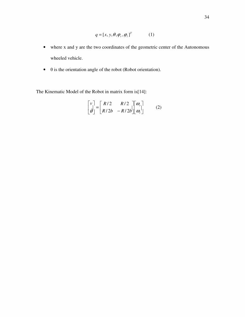
lryxq ],,,,[ ϕϕθ= (1)

• where x and y are the two coordinates of the geometric center of the Autonomous

wheeled vehicle.

• θ is the orientation angle of the robot (Robot orientation).

The Kinematic Model of the Robot in matrix form is[14]:

−=

l

r

bRbR

RRv

ω

ω

θ 2/2/

2/2/

& (2)

Chapter 4

Gradient Increase Approach

Relationship between distance from the light source and

light intensity

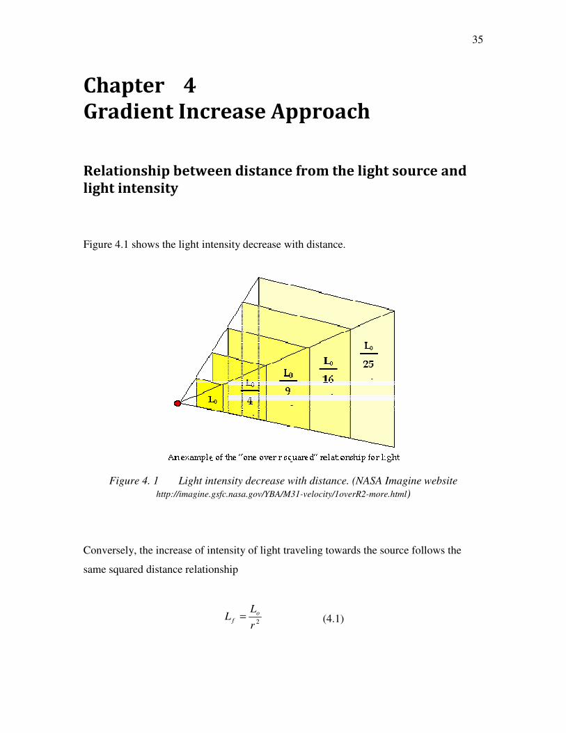
Figure 4.1 shows the light intensity decrease

Figure 4. 1 Light intensity decrease with distance. (NASA Imagine website

http://imagine.gsfc.nasa.gov/YBA/M31

Conversely, the increase of intensity of li

same squared distance relationsh

Increase Approach


ight intensity decrease with distance.

Light intensity decrease with distance. (NASA Imagine website

http://imagine.gsfc.nasa.gov/YBA/M31-velocity/1overR2-more.html)

the increase of intensity of light traveling towards the source follows the

relationship

2r

LL o

f = (4.1)

35


Light intensity decrease with distance. (NASA Imagine website

ght traveling towards the source follows the

36

When the sensors detect a light source, the value of incandescence will increase at this

squared distance relationship in terms of distance (r) moving towards the light source.

Heat can be transferred from an object in three different ways, namely, conduction,

convection and radiation. In the case of a fire source, the heat is transferred to the sensor

by radiation.

The radiated heat follows the same relationship with respect to distance from the source.

Hence the detected increase in temperature will not be very substantial but, as the

distance to the source decreases, the increase in temperature will be exponential.

To calculate that, we have to take “solid angle” in account this has the units “Stradians”

in the SI system. The conical vision of the sensors will have a detection area depending

upon the angle of vision of the sensor.

One whole sphere has about 4π Stradians. We will not go into the solid angles in detail

as we have made an assumption that the robot is detecting the fire source in a two-

dimensional environment.

Hence the distance to the source and the intensity of light are the two factors that remain

of interest.

Table 4. 1 Relationship of light intensity with distance from the source

The light coming from a luminous source can be considered as a three dimensional ball

increasing in size and decreasing in intensity

4.2 describes the relationship in a graphical manner.

It is possible for a sensor to detect the

comparing the gradient of light at different positions from a source

calculate the distance and also direction of the source.

0

5

10

15

20

1 2 3 4 5

Relationship of light intensity with distance from the source

from a luminous source can be considered as a three dimensional ball

and decreasing in intensity as it travels away from the source. Figure

4.2 describes the relationship in a graphical manner.

t is possible for a sensor to detect the robot movement relative to the source

comparing the gradient of light at different positions from a source and to permit

calculate the distance and also direction of the source.

Light Source Distance (cm)5 6 7 8 9 10 11

Light Source Distance (cm)

Intensity of Light (percent)

37

Relationship of light intensity with distance from the source

from a luminous source can be considered as a three dimensional ball

as it travels away from the source. Figure

relative to the source by

and to permit to



Intensity of Light (percent)

38

Chapter 5

Navigation Strategy

There are certain animals in the wild having sensors of different kinds. For example some

snakes have IR sensors; Bats use the reflected sound waves to map their surroundings,

path and prey. Also some insects such as beetles have shown some greatly evolved

infrared sensing of forest fires, not to escape it but to lay their eggs in freshly burnt wood.

[15]

Most of the animals including humans have two eyes, ears, hands, nostrils. That not only

gives them a “stereo sensing” of the objects in question but also a perception of “depth”.

It is very easy for humans and most other animals to just move their neck and sense the

objects around them but it becomes a more challenging when an autonomous robot has to

do the same thing.

Lilienthal et al. in his paper “Gas Source Tracing With a Mobile Robot Using an Adapted

Moth Strategy, 2003”[15] discusses different strategies adopted by different moths to

detect sources of different kinds. One silkworm insect called Bombyx Mori uses a similar

strategy. In that strategy, a fixed motion pattern realizes a local search and restarts the

motion pattern if increased source concentration is sensed.

It results in “Asymmetric motion pattern biased towards the side where higher sensor

readings are obtained hence keeping the robot in a close proximity of the source after

guiding it”.

The behavior of the silkworm moth Bombyx mori is well-investigated and suitable for

adaptation on a wheeled robot, because this moth usually does not fly. The behavior is

mainly based on three mechanisms [15]

39

� a trigger: if the moth’s antennae are stimulated by intermittent patches of phero-

mones, a fixed motion pattern is (re-)started

� local search: the motion pattern realizes an oriented local search for the next

pheromone patch

� estimation of source direction: the main orientation of the motion pattern that

implements the local search is given by the instantaneous upwind direction, which

provides an estimate of the direction to the source

Stimulation to either antenna triggers the specific motion pattern of the Bombyx males.

This fixed motion sequence starts with a forward surge directed against the local air flow

direction. Afterwards, the moth performs a “zigzag” walk, while it starts to turn to that

direction where the stimulation was sensed. The turn angles and the length of the path

between subsequent zigzag motions turns increase with each turn. Finally, a turning

behavior is performed, while the turns can be more than 360 ◦. This “programmed”

motion sequence is exactly restarted from the beginning if a new patch of pheromones is

sensed. As it could be shown in wind tunnel experiments by Kanzaki [16], this behavior

results in a more and more straightforward path directed towards the pheromone source if

the frequency of pheromone stimulation is increased. [17]

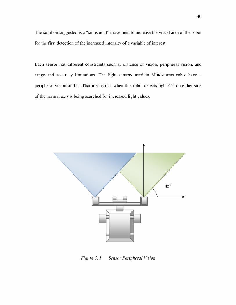
40 The solution suggested is a “sinusoidal” movement to increase the visual area of the robot

for the first detection of the increased intensity of a variable of interest.

Each sensor has different constraints such as distance of vision, peripheral vision, and

range and accuracy limitations. The light sensors used in Mindstorms robot have a

peripheral vision of 45°. That means that when this robot detects light 45° on either side

of the normal axis is being searched for increased light values.

Figure 5. 1 Sensor Peripheral Vision

45°

41

5.1 Sinusoidal or Zigzag Movement of the Robot

Introduction of the sinusoidal movement of the robot is important to scan a larger

area for possible heat and light sources.

Figure 5. 2 Sinusoidal movement of the robot and scannable angles

Since the sensors are fixed on the robot and the movement of robot determines the

direction of these sensors, the vision of these sensors is limited to 45˚. The sinusoidal

movement used for the navigation strategy, moves the robot 45˚ to the right and 45˚ to

the left while sampling the elevated levels of light or heat. This sinusoidal movement,

shown in Figure 5.2, requires peripheral vision of sensors of 180˚ in the direction of

motion of the robot.

In order to cover 180˚ in the direction of motion it was chosen to use a scanning approach

such that, as the robot travels in a straight line, the sensors cover the area surrounding it.

DIRECTION OF MOTION

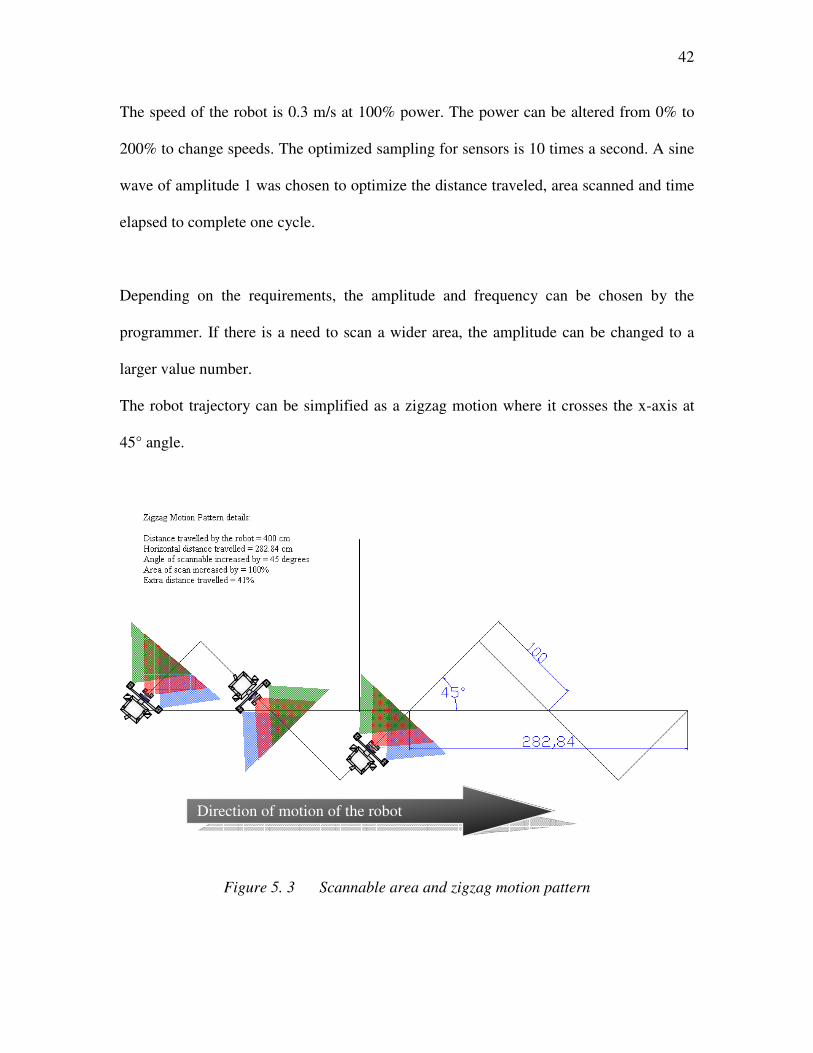
42 The speed of the robot is 0.3 m/s at 100% power. The power can be altered from 0% to

200% to change speeds. The optimized sampling for sensors is 10 times a second. A sine

wave of amplitude 1 was chosen to optimize the distance traveled, area scanned and time

elapsed to complete one cycle.

Depending on the requirements, the amplitude and frequency can be chosen by the

programmer. If there is a need to scan a wider area, the amplitude can be changed to a

larger value number.

The robot trajectory can be simplified as a zigzag motion where it crosses the x-axis at

45° angle.

Figure 5. 3 Scannable area and zigzag motion pattern

Direction of motion of the robot

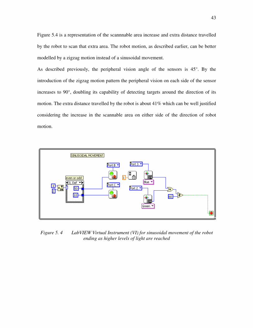
43 Figure 5.4 is a representation of the scannnable area increase and extra distance travelled

by the robot to scan that extra area. The robot motion, as described earlier, can be better

modelled by a zigzag motion instead of a sinusoidal movement.

As described previously, the peripheral vision angle of the sensors is 45°. By the

introduction of the zigzag motion pattern the peripheral vision on each side of the sensor

increases to 90°, doubling its capability of detecting targets around the direction of its

motion. The extra distance travelled by the robot is about 41% which can be well justified

considering the increase in the scannable area on either side of the direction of robot

motion.

Figure 5. 4 LabVIEW Virtual Instrument (VI) for sinusoidal movement of the robot

ending as higher levels of light are reached

44

Figure 5. 5 Flow chart for the zigzag movement of robot

As previously described, the program written in LabVIEW is called a Virtual Instrument

or a VI. In the above VI designed for sinusoidal movement several issues were

considered. The motors of the robot are running at a predefined speed, changing their

direction as the speeds of the motors are changed. For the first second, Motor B runs at

50% power while Motor C runs at 10% power essentially turning the robot right. After

that one second, the same ratio is applied to the motors but it is reversed, moving the

robot in the other direction, achieving a sinusoidal curve of amplitude of 1.

Two light sensors can also be observed detecting light. The sensor connected to

Port 2 emits green light and the sensor connected to Port 3 emits blue light for

recognition purposes. If one of these sensors detects light value more than or equal to 60

Lumens, this sinusoidal movement program terminates bringing the robot to halt. But the

Start Navigation

Go forward 200

cm reading light

sensor

Make a 90 right

turn reading light

sensor

Go forward 200

cm reading light

sensor

Make a 90 left

turn reading light

sensor

Stop Navigation if

light reading is

above 60 lumens

45 next level of program comes into effect which guides the robot towards the now-detected

light or heat source. That strategy is discussed in Chapter 7.

Next, a description is given for tracking of the light source with one, two and

three sensors. The information given in this chapter only refers to the tracking and

approach of the robot to the source. Fire declaration algorithms are described later in

Chapter 6 and 7.

5.2 Tracking of a heat source with one sensor

In the case of a single sensor tracking, the way to follow the increasing gradient of heat

was to compare the current temperature reading with previous reading. As mentioned in

Chapter 4, the gradient of light and heat would increase if the robot is approaching the

source. Hence a program was designed to make the robot go straight as long as the

current temperature was greater than the previous one. As soon as the comparison shifted

the other way around or gave the same temperature reading as the previous reading, the

robot would slightly turn right (or left). If the comparison continues to give lower or

equal values, the robot will keep on going in a circle until it detects elevated temperature

values and starts travelling towards it.

The TIR sensor was mounted in the front of the robot. TIR sensor gives the object

temperature function of distance. As described in Chapter 4, the relationship between the

light or temperature intensity increase to the distance is exponential.

46 For this purpose a “While loop with Shift Register” was used. The strategy developed

was that the motors A and B would make the robot make a 360° turn. On the detection of

elevated temperature, both motors start moving and drive the robot towards frontward.

Temperature readings are taken every 100th of a second. These readings are compared to

the previous temperature readings which makes the robot decide if it needs to go straight

or turn.

To maximize the certainty and minimize jerky motion of the robot, an average of the last

4 readings is taken in account to be compared to the current value, producing a much

smoother curve and hence smooth movement.

By comparing the previous readings and always going towards the higher reading than

the previous one, the robot is able to get to the source. A predefined temperature value

determines that the robot has approached close enough to the source and at that point it

beeps and stops moving.

47

Figure 5. 6 LabVIEW programming for a while loop with shift register showing the

true case of increasing gradient of object temperature

As it can be seen from the simple programming that the TIR sensor is connected

to the brick via port 1. There are two charts produced by this program. One shows the

current raw value of temperature detected by the sensor in degree Celsius and the other

chart displays the average of the last four values of the temperatures to make the chart

smoother. The case structure has the capability to return different values if a true or a

false value is provided to it as input. The stop button terminates the program. It can also

be connected to a specific situation as it is reached when the program may stop, such as

the achievement of a high temperature to declare a fire incident.

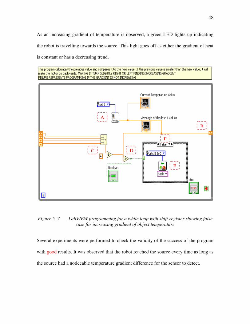
48 As an increasing gradient of temperature is observed, a green LED lights up indicating

the robot is travelling towards the source. This light goes off as either the gradient of heat

is constant or has a decreasing trend.

Figure 5. 7 LabVIEW programming for a while loop with shift register showing false

case for increasing gradient of object temperature

Several experiments were performed to check the validity of the success of the program

with good results. It was observed that the robot reached the source every time as long as

the source had a noticeable temperature gradient difference for the sensor to detect.

A

B

E

DC

F

Figure 5. 8 Block diagram for one sensor gradient increase VI

In this particular experiment

any obstacles in the way. Hence the obstacle avoidance techniques were not used. The

speed of the robot was kept at 50% to allow

not miss readings.

The waiting time for each reading was one tenth of a second, way below the

sensor capacity to make sure that the sensor does not return an indefinite value.

Gradient Decrease?

(E)

Turn right for 0.5

seconds

(F)

Block diagram for one sensor gradient increase VI

the robot was placed in the plain sight of the source without

Hence the obstacle avoidance techniques were not used. The

speed of the robot was kept at 50% to allow enough time to detect the temperature and

time for each reading was one tenth of a second, way below the

y to make sure that the sensor does not return an indefinite value.

Get light intensity

values from the

sensor (A)

Fig 5.3

Get the current

value of light

intensity (B)

Compare light

values from the

average of previous

4 values (D)

Gradient Decrease?

(E)

Turn right for 0.5

seconds

(F)

Gradient Increase?

(E)

Go forward

(F)

Get previous four

values of light

intensity and divide

it by 4 (C)

49

Block diagram for one sensor gradient increase VI

the robot was placed in the plain sight of the source without

Hence the obstacle avoidance techniques were not used. The

time to detect the temperature and

time for each reading was one tenth of a second, way below the

y to make sure that the sensor does not return an indefinite value.

50 As evident from Figure 5.5, the robot continuously followed the increased gradient of

temperature until it reached a peak value of 130°C, which had been pre-defined as the

declaration of fire.

Figure 5. 9 Temperature waveform for the single sensor based increasing gradient

trail guidance

If the waveform was to be looked at critically it can be observed that there are

some points in the curve where the temperature was steady for a brief moment of time

such as at 95°C and 126°C. Also another observation could be made for the temperature

actually reducing at 114°C, 128°C and 120°C. but other than these points the gradient

followed is always increasing.

Also from 80°C to 95°C the curve is exponential which at a constant speed

signifies that the robot was traveling straight towards the heat source. When the reflected

temperatures come into effect as the robot approaches closer to the source it can be

51 observed that the robot had to correct its direction to find the highest possible value in its

area of scanning. It took the robot 10 seconds to reach the goal.

Certain amplitudes and frequencies were tested and a mean value was reached

that produced accurate detection of the source (giving enough time to the sensors to track

the light source) while not exhausting the batteries at a faster rate.

Tangents were drawn at 45˚ on the chart to find out that the actual area covered

was 180˚. Moving in the sinusoidal movement not only eliminates the chances of the

robot travelling to a point that is reflecting the signal in question but also makes sure that

other sources are also kept under consideration.

5.3 Tracking of the source with TWO sensors

Tracking of a light source with two sensors gives us an opportunity for a strategy of a

continuous comparison between the sensor readings is and, depending upon the sensor

reading values, for a robot control that can change its direction of movement.

52

Figure 5. 10 Two light-sensor tracking system

Essentially the two sensor readings are compared by using a comparison operator. In

Figure 5.6 the peripheral visual range of the sensors is described but the ambient and

reflected light does reach the sensor as well. The robot successfully reaches the source by

NXT 2.0

Sensor S1 Sensor S2

NXT 2.0

Sensor S1 Sensor S2

53 repeating the commands until a termination condition such as a stop button or intensity of

light above a certain value is reached.

Figure 5. 11 VI for two sensor source approaching

As the two sensors are connected to two different ports, they are defined by the color of

light their lamp emits and the position of port they are connected to. The motors are also

defined by the name of port they are connected to. For data acquisition two charts are

also connected to the raw data so that the observer can log the data. For the comparison

operator, a greater or equal operator is used. The reason for this operator being used is

that if the readings of both sensors at any given scenario are equal, the robot moves and

creates an unequal reading from these sensors hence avoiding indeterminate points while

approaching the source of light.

A

B

B

Figure 5. 12

The front panel from Fig. 5.10

representation of the approach towards the light.

Figure 5. 13 Front Panel for two

Light value of the

right sensor is

greater than the left sensor (B)

Go right going

forward

Gradual increase of light values. Comparison can be seen on both readings

Block diagram for two-sensor light following

10 of this virtual instrument (VI) gives a graphical

representation of the approach towards the light.

Front Panel for two-sensor light tracking system

Compare light

values from the

two sensors (Fig 5.7) (A)

Light value of the

right sensor is

greater than the left sensor (B)

Go right going

forward

Light value of the

left sensor is equal

to or greater than the right (B)

Go left going

forward

54

of this virtual instrument (VI) gives a graphical

r light tracking system

55

Figure 5.8 shows the sensor readings as the robot travels in a zigzag motion leaning

towards a higher gradient of light and finally approaching it. For this experiment the

robot was placed in a dark room with one light source while it detected and approached

it.

5.4 Obstacle Avoidance One of the major ingredients of a robot program is obstacle avoidance. This is

particularly necessary for the robot to be in a good shape to perform different actions.

SONAR or Ultrasonic sensor was used for obstacle avoidance in these

experiments. Simple avoidance would consist of three steps

• Scan the area for any obstacles

• When an obstacle is detected within a pre-defined distance, either change

direction or back up

• Continue to scan for variables of interest after performing these actions.

In the current deployment of the VI’s it was important that the robot does not waste time

in trying to figure out which way to turn hence the two light sensors on either side help

the robot making a choice of direction to back up too.

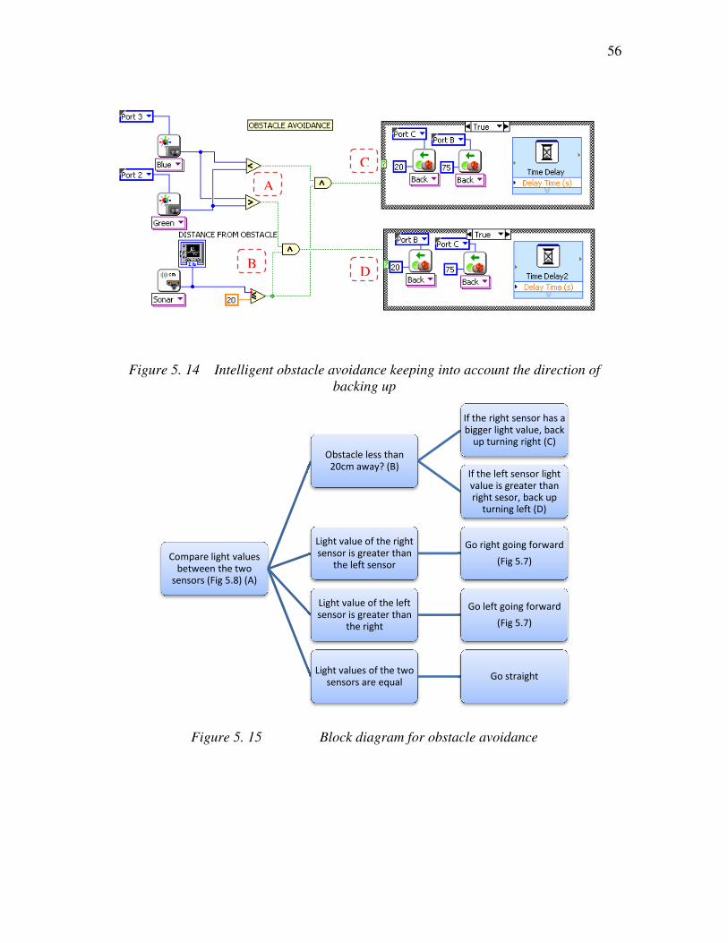
Figure 5. 14 Intelligent obstacle avoidance keeping into account the direction of

Figure 5. 15

Compare light values

between the two

sensors (Fig 5.8) (A)

A

B

Intelligent obstacle avoidance keeping into account the direction of

backing up

Block diagram for obstacle avoidance

Obstacle less than

20cm away? (B)

If the right sensor has a

bigger light value, back

up turning right (C)

If the left sensor light

value is greater than

right sesor, back up

turning left (D)

Light value of the right

sensor is greater than

the left sensor

Go right going forward

(Fig 5.7)

Light value of the left


the right

Go left going forward

(Fig 5.7)

Light values of the two

sensors are equalGo straight

A

C

D

56

Intelligent obstacle avoidance keeping into account the direction of







turning left (D)



57 As the robot approaches an obstacle the ultrasonic sensor S4 comes into control of the

motors. At this point the robot would back up not going straight backwards but detects

the light values from the two light sensors.

Figure 5. 16 Obstacle Avoidance

If Sensor S1 receives a higher value of light than the sensor S2, it would back up turning

towards the direction of the sensor S1 and if the sensor S2 is displaying a higher reading,

it would turn towards the direction while backing up, towards the sensor S2.

Obstacle 1

Obstacle 2

Obstacle 3

Figure 5. 17 Front panel results for obstacle avoidance with record of temperature

Obstacle more than 255 cm away temperature values

Front panel results for obstacle avoidance with record of temperature

readings

Gradual increase in

temperature values

Following

increasing light

Approaching the obstacle

Obstacle avoided

Target is also an obstacle

Fire Declaration

58

Front panel results for obstacle avoidance with record of temperature

Gradual increase in

temperature values

Following

increasing light

Approaching the

Obstacle avoided

Target is also an obstacle

59

Chapter 6

Voting Logic Fusion

6.1 Introduction As evident from its name, Voting Logic Fusion is a sensor fusion technique that

takes all the sensors and their level of readings into account in the source declaration

process. It is a very useful technique to detect, track and classify objects. This technique

provides superior protection against false alarms in a high clutter or noisy background. A

detailed description of this technique is given in the book “Sensor and Data Fusion: A

Tool for Information Assessment and Decision Making” by Lawrence A Klein [18] .

Different sensor arrangements have different advantages and disadvantages. For

example a parallel configuration of the sensors means that each sensor is working

independently and the decision making process does not depend on other sensors

readings. This arrangement is especially very efficient in detecting the suppressed or

noisy targets. For this sensor arrangement, extra care must be taken to choose the sensors

as it requires sophisticated and accurate sensors, increasing the cost of the assembly. Also

this type of arrangement is susceptible to false alarms, as at one time only one sensor is

responsible for declaration of the targets. Hence it is easy to distract a robot with this type

of sensor arrangement.

60

Figure 6. 1 Parallel sensor arrangement [18]

Venn Diagram for the parallel arrangement appears to be as follows:

Figure 6. 2 Venn diagram for parallel sensor arrangement [18]

Series configuration, on the other hand requires all the sensors to declare a target

simultaneously for the system to announce declaration. The advantages of this system are

reverse of the parallel configuration. This configuration is very good in rejecting false

alarms from decoys but on the other hand this system does not exhibit a good suppressed

target declaration. This configuration does not require extremely high quality sensors

hence the cost of the system is low.

Figure 6. 3 Series sensor arrangement with Venn diagram[18]

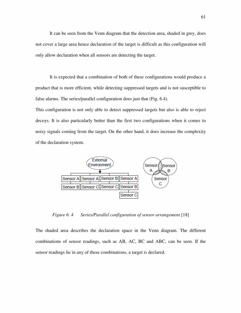
61 It can be seen from the Venn diagram that the detection area, shaded in grey, does

not cover a large area hence declaration of the target is difficult as this configuration will

only allow declaration when all sensors are detecting the target.

It is expected that a combination of both of these configurations would produce a

product that is more efficient, while detecting suppressed targets and is not susceptible to

false alarms. The series/parallel configuration does just that (Fig. 6.4).

This configuration is not only able to detect suppressed targets but also is able to reject

decoys. It is also particularly better than the first two configurations when it comes to

noisy signals coming from the target. On the other hand, it does increase the complexity

of the declaration system.

Figure 6. 4 Series/Parallel configuration of sensor arrangement [18]

The shaded area describes the declaration space in the Venn diagram. The different

combinations of sensor readings, such as AB, AC, BC and ABC, can be seen. If the

sensor readings lie in any of these combinations, a target is declared.

62 This type of sensor arrangement supports a Voting Logic Fusion process. In this

process, the user gets the best of both the worlds. It allows the sensors to automatically

detect and classify targets based on the knowledge gained by sensing. This process also

does not require manual switching of the sensors based on the quality of their inputs

rather this system has the ability to understand different levels of signatures in different

combinations. This configuration may also be modified to suit the needs of another

current project. Some predefined conditions may also be added in the rules of

declarations.

The fusion algorithm combines the target report data and assesses the likelihood of the

target being present at any location. The characteristics of the sensor inputs such as

spatial frequency, amplitudes and bandwidth play a significant role in fusion algorithm.

6.2 Confidence Levels

Each sensor has a degree to which the signal conforms to pre-defined target

characteristics. The amount to which an output signal complies with the pre-defined

characteristics of the potential target, determines the confidence level of the sensor report.

The confidence level is dependent not only on the sensor qualities but also the target

characteristics. So it can be said that the confidence level is dependent on the degree of

which an input signal matches an ideal target, the pre-identified value that matches to the

ideal target and signal to interference ratio.

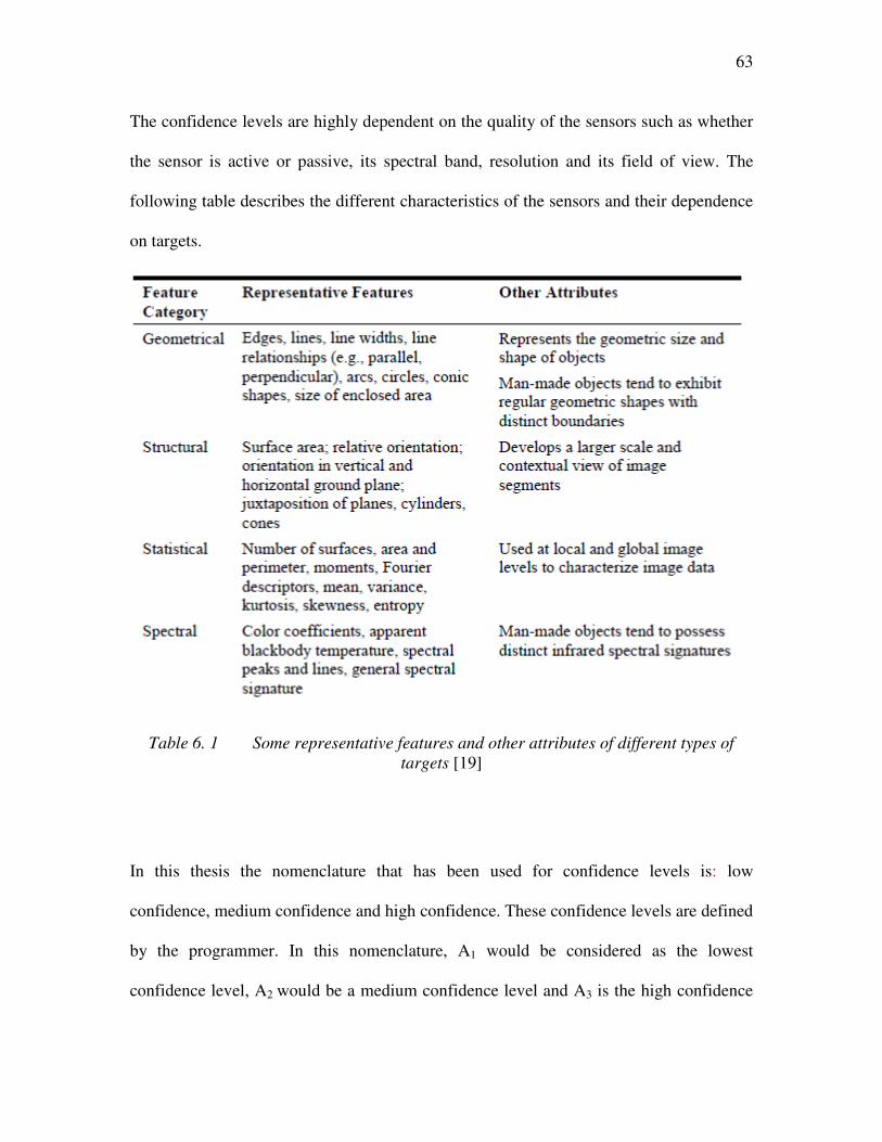
63 The confidence levels are highly dependent on the quality of the sensors such as whether

the sensor is active or passive, its spectral band, resolution and its field of view. The

following table describes the different characteristics of the sensors and their dependence

on targets.

Table 6. 1 Some representative features and other attributes of different types of

targets [19]

In this thesis the nomenclature that has been used for confidence levels is: low

confidence, medium confidence and high confidence. These confidence levels are defined

by the programmer. In this nomenclature, A1 would be considered as the lowest

confidence level, A2 would be a medium confidence level and A3 is the high confidence

64 level. Later in the next chapter there has been an introduction of the confidence level A4

which will be discussed in detail while examining the modification of the voting logic.

Same nomenclature can be adopted for the other sensors with a subscript of the level of

confidence.

6.3 Detection Modes Detection modes may be defined as the combinations of sensor outputs that may be

considered as the presence of a valid target declaration. In a typical detection mode the

user may define a combination of the lowest confidence level detected by all the sensors

detecting the target, or it may include one sensor with high confidence level and two with

intermediate or low confidence levels.

In a three-sensor detection system, if the sensor nomenclature was to be considered as A,

B and C and the confidence levels are defined as subscript 1 for the lowest and 3 for the

highest confidence level, the combinations that are attained are discussed in table 6.2.

As it can be clearly seen from the combinations that a variety of possible combinations is

present and the combinations of interest may only be defined by the user as deciding

combinations for declaration of the target.

There are 27 i.e., (33 or 3x3x3) combinations for the three sensor system with three

confidence levels as described in Table 6.2. They range from the lowest confidence levels

to the highest confidence levels.

65

Also Tables 6.3, 6.4 and 6.5 detail the possible combinations for the two sensor

combinations. Nine possible combinations i.e. (32) describe detection modes for two

sensor combination.

Out of these possible combinations detection modes may be defined. For example if a

detection mode for three sensors is to be defined as a combination of at least low

confidence level reading from all these sensors may be considered to be a detection

mode. Also for two sensor combinations, at least medium confidence from both of the

sensors may be defined as a possible detection mode. In different cases different

combinations are required for detections.

Combination of sensors Possible combinations of confidence levels

ABC

A1B1C1

A1B1C2

A1B1C3

A1B2C1

A1B2C2

A1B2C3

A1B3C1

A1B3C2

A1B3C3

66

A2B1C1

A2B1C2

A2B1C3

A2B2C1

A2B2C2

A2B2C3

A2B3C1

A2B3C2

A2B3C3

A3B1C1

A3B1C2

A3B1C3

A3B2C1

A3B2C2

A3B2C3

A3B3C1

A3B3C2

A3B3C3

Table 6. 2 Three sensor combinations when all sensors inputs are obtained


AB A1B1

67

A1B2

A1B3

A2B1

A2B2

A2B3

A3B1

A3B2

A3B3

Table 6. 3 Two sensor combinations for sensors A and B


AC

A1C1

A1C2

A1C3

A2C1

A2C2

A2C3

A3C1

A3C2

A3C3

Table 6. 4 Two sensor combinations for sensors A and C

68


BC

B1C1

B1C2

B1C3

B2C1

B2C2

B2C3

B3C1

B3C2

B3C3

Table 6. 5 Two sensor combinations for sensors B and C

These choices highly depend upon the inherent qualities of the sensors. So in a

typical case where sensor A has a higher probability of detection, the confidence level of

sensor A required to declare a target may not require the highest possible level when in

combination with other sensors. An example of the declaration modes is provided in the

following table 6.6

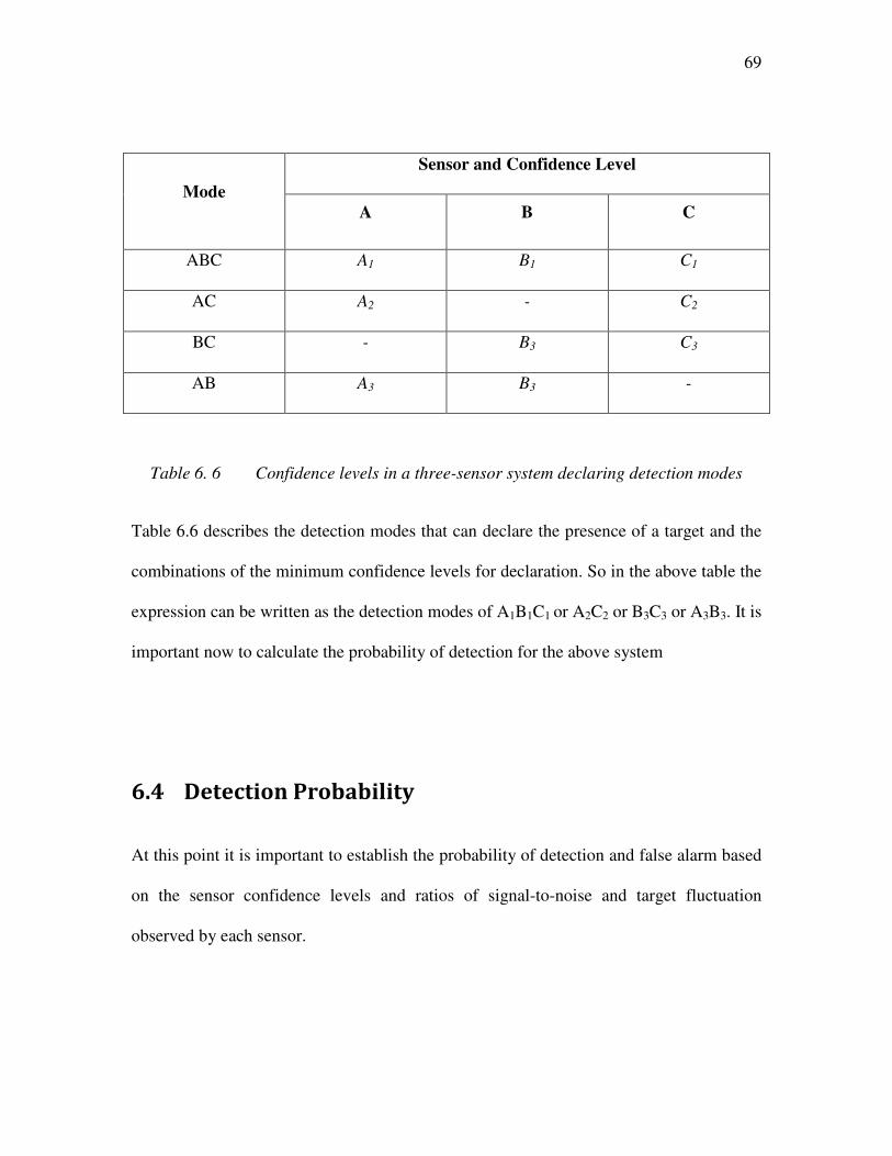
69

Mode

Sensor and Confidence Level

A B C

ABC A1 B1 C1

AC A2 - C2

BC - B3 C3

AB A3 B3 -

Table 6. 6 Confidence levels in a three-sensor system declaring detection modes

Table 6.6 describes the detection modes that can declare the presence of a target and the

combinations of the minimum confidence levels for declaration. So in the above table the

expression can be written as the detection modes of A1B1C1 or A2C2 or B3C3 or A3B3. It is

important now to calculate the probability of detection for the above system

6.4 Detection Probability

At this point it is important to establish the probability of detection and false alarm based

on the sensor confidence levels and ratios of signal-to-noise and target fluctuation

observed by each sensor.

70

6.4.1 Derivation of system detection and false-alarm probabilities

Using these confidence level combinations (detection modes) Boolean algebra may be

used to derive the system detection and system false-alarm probabilities. As described in

the previous section, there are one three-sensor and three two sensor detection modes.

The system probability would be the sum of the individual probabilities of each detection

mode. As an illustration, based on the expert knowledge of the designer, it will be

considered the following logic combination

A3B3C3 OR A2C2 OR B1C1 OR A1B1

gives the equation for system probability of detection

System Pd = Pd{A3B3C3 OR A2C2 OR B1C1 OR A1B1} (6.1)

This equation may be expanded by repeated application of the Boolean algebra

expression given as

P{X OR Y} = P{X} + P{Y} – P{XY} (6.2)

The equation 6.1 then gets expanded as follows

System Pd = Pd{A3B3C3} + Pd{A2C2} + Pd{B1C1} +

Pd{A1B1} - Pd{A3B3C1A2C2} - Pd{A3B3C3B1C1} -

Pd{A3B3C3A1B1} - Pd{A2B2B1C1} – Pd{A2C2A1B1} –

Pd{B1C1A1} + Pd{A3B3C3A2C2B1C1} +

Pd{A3B3C3A2C2A1B1} + Pd{A3B3C3B3C1A1B1} +

(6.3)

71

Pd{A2C2B1C1A1B1} + Pd{A3B3C3A2C2B1C1A1B1}

These are non-nested sensors so the confidence levels of each sensor is independent of

others, hence the expression for union and intersection that are applicable are as follows:

Pd{A1 U A2} = Pd{A1}+ Pd{A2} (6.4)

And

Hence the simplified system detection probability expression becomes:

As each sensor is independent of the readings of the other sensors, the probability of

detection may be written as the product of the probability of detection from each sensor.

This yield:

Equation 6.7 describes the total system probability of detection as the product of

the detection probabilities of sensors A, B and C at the lowest confidence level added to

the product of probability of detection of the sensors A and B at the medium confidence

Pd{A1 ∩ A2} = 0 (6.5)

System Pd = Pd{A3B3C3} + Pd{A2C2} + Pd{B1C1} + Pd{A1B1} -

Pd{A1B1C1} (6.6)

System Pd = Pd{A3} Pd {B3} Pd {C3} + Pd{A2} Pd {C2} +

Pd{B1} Pd {C1} + Pd{A1} Pd {B1} - Pd{A1} Pd {B1} Pd {C1} (6.7)

72 levels added to the product of probability of detection of sensors A and C at the highest

confidence level, subtracted by the product of detection probabilities of sensors A, B and

C at the highest confidence level.

Meanwhile as each system has a false alarm probability, it is as important to

calculate the false alarm probability as it is to calculate the detection probability. The

same equation, (Equation 6.7) may be used to detect false alarm probability of the system

as well. [18]

Where “System Pfa” is the false alarm probability of the system.

6.4.2 System detection probability

Using the values from three sensors, two of which are light and color sensors, and one of

them is temperature sensor. The individual sensor detection probability at a particular

confidence level is calculated by multiplying the inherent detection probability of that

sensor by the conditional probability. Then the modal detection probability is calculated

by multiplication of sensor detection probabilities

System Pfa = Pfa{A3} Pfa {B3} Pfa {C3} + Pfa{A2} Pfa {C2} +

Pfa{B1} Pfa {C1} + Pfa{A1} Pfa{B1} – Pfa{A1} Pfa {B1} Pfa {C1} (6.7)

73

These are the steps to follow while computing the detection probability

� Determination of the detection modes

� Selection of inherent false alarm probabilities for each sensor confidence level

� Calculation of the conditional probabilities corresponding different confidence

levels by performing offline experiments.

� Calculation and verification of false alarm probabilities

� Calculation of the inherent false alarm probabilities of each sensor

� Calculation of the inherent detection probabilities of each sensor

� Calculation of the probabilities of target detection by each sensor at appropriate

confidence level

� Computation of system detection probability

� Computation of system false alarm probability

� Verification of the satisfaction of the requirements

74

Chapter 7

Modified Voting Logic Fusion

7.1 Introduction:

Voting logic, as described in Chapter 6, is the process of declaration of a source that

keeps into account the values, confidence levels and algorithms of all participating

sensors. This system has great deterrence against non detection and false alarms. In order

to improve on the currently available voting logic system, there are certain modifications

that may be made. Even though this system exhibits a great flexibility, there is still the

possibility of non-detection and false alarm.

Depending upon the type of sensors, certain logic rules may be implemented that

are necessarily not part of voting logic to use these sensors more efficiently.

7.2 Single Sensor Detection Modes The current thesis focuses on fire detection in an industrial environment. Fire

exhibits certain qualities that may be clues for declaration of a fire source. Some of these

variables are more important part of declaration process than others. For example a fire

would

• Sometimes generate smoke

• Most often generate light

75

• Always generate heat

• Always produce CO2

The presence of only smoke or light may not be enough evidence to declare fire.

Also CO2 is normally found in the atmosphere and the fire may not be the only source to

produce that gas if elevated levels of Carbon Dioxide are detected. That could be because

of people breathing in a closed environment or a manufacturing process.

Heat, on the other hand, if above certain threshold, maybe enough evidence of a

threatening situation provided there are no controlled fires present in that area, such as a

forging shop or a heat treatment shop. In heat treatment shops normally the temperatures

are inside the kiln and outside temperatures are normal.

Therefore it is fitting to include the singleton sensor detection modes in fire

declarations for the industrial environment[11] Current hardware did not allow the use of

smoke or CO2 sensors so two light sensors and one heat sensor was used in the first batch

of experiments.

A fire declaration is possible in the current circumstances when we have the light

readings above threshold and the temperature above a certain level. The possibility of fire

diminishes if the light sensors are providing a reading that is higher but the robot does not

detect elevated temperatures. The robot may reach close to the target where due to robot

geometry the light sensors may not give a reading that falls in any confidence level but it

76 has approached the source. At that instance the sensor A will give the highest confidence

level due to the temperature present but since the other sensors are not able to sense it,

voting logic will not declare a target based on the output of just one sensor.

Figure 7. 1 Possible combinations of sensor readings

At this point the reading from the other sensors becomes irrelevant. Normal voting logic

does not keep this scenario into account. Whereas in order to reach the point of interest

the robot has to follow any lead of increased light only and will not declare the fire

source until it reaches a point where elevated temperatures are also detected.

Hence single sensor detection mode was introduced in this chapter which marks

one modification of the mode. In the following in this thesis, sensor A, as described by

the temperature sensor (TIR), the confidence level A1 will always declare fire, as it may

be the deciding factor due to robot geometry or type of fire. As an illustration, based on

the expert knowledge of the designer, it will be considered the following logic

combination of the detection modes ehich gives the following equation for system

ABC

AC AB

A B C

77

7.2.1 Visual Representation of these detection modes

Figure 7. 2 Fire present at First detection mode A1

Figure 7. 3 Fire present at First detection mode A2B2

A1 or A2B2 or A2C2 or A3B1C2 or A3B2C1 (7.1)

ABC

AC AB

A B C

ABC

AC AB

A B C

78

Figure 7. 4 Fire present at First detection mode A2C2

Figure 7. 5 Fire present at First detection mode A3B1C2

ABC

AC AB

A B C

ABC

AC AB

A B C

79

Figure 7. 6 Fire present at First detection mode A3B2C1

7.2.2 Single Sensor Non-Possibility Mode As in section 7.2 different detectable fire characteristics were described, one of

which is that it is not possible to have a fire while the temperatures are low. There could

be a presence of light, Carbon Dioxide, smoke but if there is no heat present, it can be

safely said that there is no fire present, as smoke and CO2 may have been generated from

other processes and light is always present in any workshop.

Hence it is also fitting to say that a single sensor may not only be a deciding

factor in a declaration but also the same sensor may imply that a fire occurrence is not

possible., as clear from the name, single sensor non possibility mode. In this case the

ABC

AC AB

A B C

80 algorithm will ignore any combination of detection probabilities while elevated

temperatures are not detected.

In the description to follow, the confidence level introduced as A4 will declare the

non-possibility of fire.

The nomenclature for the subscript numbers for sensor A are:

A1 = Highest confidence (Single sensor declaration level confidence)

A2 = High confidence

A3 = Medium confidence

A4 = Low confidence (Single sensor non-declaration level confidence)

The reason for adoption of this nomenclature even though, different from the one

provided in the previous chapter is the introduction of A4, the non-possibility confidence

level.

The significance of this single sensor non-possibility mode becomes more practical

where there is a need to reduce calculation pressure on a CPU while there are many other

combinations that it has to compute, all the combinations with single sensor non

possibility mode may be ignored, increasing the efficiency and performance of the CPU.

It is also a very practical solution for a limited capability robot that may increase its

performance.

81

7.2.3 Derivation of Single Sensor System Pd

Equation 6.1 can be used to describe the Probability of detection of a sensor system. As

we have a different combination of detection modes in this case, the equation can be

modified to become

System Pd = Pd{ A1 or A2B2 or A2C2 or A3B1C2 or A3B2C1} (7.2)

A point to be noted here is that there is no combination having A4 present, which

automatically declares the non-possibility of the declaration of fire.

This equation may be expanded by repeated application of the Boolean algebra

expression given as

P{X OR Y} = P{X} + P{Y} – P{XY} (6.2)


System Pd = Pd{A1} + Pd{A2B2} + Pd{A2C2} + Pd{A3B1 C2}

+Pd{A3B2 C1}

– Pd{ A1 A2B2} – Pd{ A1 A2C2}} – Pd{ A1 A3B1 C2} – Pd{ A2B2 A2C2}

– Pd{ A2B2 A3B1 C2} – Pd{ A2B2 A3B2 C1} – Pd{ A2C2 A3B1 C2}

– Pd{ A2C2 A3B2 C1} – Pd{ A3B1 C2 A3B2 C1}

+ Pd{ A1 A2B2 A2C2} + Pd{ A1 A2B2 A3B1 C2} + Pd{ A1 A2B2 }

(7.3)

82

+ Pd{ A2B2 A2C2 A3B1 C2} + Pd{ A2B2 A2C2 } + Pd{ A2C2 A3B1 C2 A3B2

C1}

–Pd{ A1 A2B2 A2C2 } – Pd{ A1 A2B2 A2C2 A3B2 C1}

– Pd{ A2B2 A2C2 A3B1 C2 A3B2 C1}+ Pd{ A1 A2B2 A2C2 A3B1 C2 A3B2 C1}

These are non-nested sensors so the confidence levels of each sensor is independent of

others, hence the expression for union and intersection that are applicable are as follows:

Pd{A1 U A2} = Pd{A1}+ Pd{A2} (6.4)

And


As each sensor is independent of the readings of the other sensors, the probability of

detection may be written as the product of the probability of detection from each sensor.

This yield:

Pd{A1 ∩ A2} = 0 (6.5)

System Pd = Pd{A1} + Pd{A2B2} + Pd{A2C2} + Pd{A3B1 C2}

+Pd{A3B2 C1} (7.4)

System Pd = Pd{A1} + Pd {A2 } Pd {B2} + Pd{A2} Pd {C2} (7.5)

83

Equation 7.4 describes the total system probability of detection as the product of

the detection probabilities of sensors A, B and C at the lowest confidence level added to

the product of probability of detection of the sensors A and B at the medium confidence

levels added to the product of probability of detection of sensors A and C at the highest

confidence level, subtracted by the product of detection probabilities of sensors A, B and

C at the highest confidence level.

The numerical values in tables 7.1-7.4 are assumed typical values just for illustrating the

approach.

Meanwhile as each system has a false alarm probability, it is as important to

calculate the false alarm probability as it is to calculate the detection probability. The

same equation, (Equation 6.7) may be used to detect false alarm probability of the system

as well. [18]

Where “System Pfa” is the false alarm probability of the whole system after the algorithm

is deployed.

Tables 7.1 to 7.9 contain illustrative numerical values for testing the how the proposed

algorithms work.

+ Pd{A3} Pd {B1 } Pd {C2} +Pd{A3} Pd {B2 } Pd {C1}

System Pfa = Pfa{A1} + Pfa{A2} Pfa{B2} + Pfa{A2} Pfa{C2}

+ Pfa{A3} Pfa{B1 } Pfa{C2} + Pfa{A3} Pfa{B2 } Pfa{C1}

(7.6)

84

Sensor

Confidence

Level

Sensor A Sensor B Sensor C

A1 A2 A3 A4 B1 B2 B3 C1 C2 C3

Detection

distribution 350 550 800 1000 400 600 1000 400 600 1000

Conditional

probability 0.35 0.55 0.8 1.0 0.4 0.6 1.0 0.4 0.6 1.0

Table 7. 1 Distribution of detections among sensor confidence levels

Inherent detection probabilities calculated for the sensors at the different confidence

levels, as described in Equation 6.8

Table 7. 2 Inherent detection probabilities among sensor confidence level

To calculate the system probability of detection (System Pd), the values from the above

tables are inserted in equation 7.5, which yields:

System Pd = 0.981

System detection probability at 98.1% is a valuable result, where the possibility of non-

detection is less than 2%.

Sensor

Confidence

Level


A1 A2 A3 A4 B1 B2 B3 C1 C2 C3

Inherent

Detection

Probability

0.9 0.84 0.8 0.74 0.88 0.81 0.73 0.88 0.81 0.73

System Pd = Pd{A1} + Pd {A2 } Pd {B2} + Pd{A2} Pd {C2}

+ Pd{A3} Pd {B1 } Pd {C2} +Pd{A3} Pd {B2 } Pd {C1} (7.5)

System Pd = 0.315 + (0.46 × 0.486) + (0.46 × 0.486)

+ (0.64 × 0.352 × 0.486) +(0.64 × 0.352 × 0.486) (7.7)

85

Similarly the calculations can be done for the false alarm probability of the system.

Equation 7.6 provides the expression for false alarm calculations, as

Table 7. 3 Inherent false alarm probability for sensor A for all four confidence levels

Table 7. 4 Inherent false alarm probabilities for sensors B and C

System Pfa = Pfa{A1} + Pfa{A2} Pfa{B2} + Pfa{A2} Pfa{C2}

+ Pfa{A3} Pfa{B1 } Pfa{C2} + Pfa{A3} Pfa{B2 } Pfa{C1}

(7.6)

Sensor Confidence

Level

Sensor A

A1 A2 A3 A4

Inherent false alarm

Probability (Pfa') 1.06×10-4 1.8×10-3 1.4×10-3 1.01×10-2

Sensor Confidence

Level

Sensor B Sensor C

B1 B2 B3 C1 C2 C3


Probability(Pfa') 3.5×10-4 2.0×10-3 1 ×10-3 3.5×10-4 2.0×10-3 1 ×10-3

86 Taking the values from tables 7.3 and 7.4 into account, and using them to solve equation

7.6, the total system false alarm probability is obtained.

System Pfa = (1.06×10-4×0.9) + (1.8×10-3×2.0×10-3) + (1.8×10-3×2.0×10-3)

+ (1.4×10-3) × (3.5×10-4) × (1 ×10-3) + (1.4×10-3) × (1 ×10-3) × (3.5×10-4)

System Pfa = (9.54 ×10-5) + (4.32×10-6) + (4.32×10-6) + (4.9×10-10) + (4.9×10-10)

System Pfa = 1.0 ×10-4

7.3 Two-sensor Detection and Non-Possibility Modes Also depending upon the choice of sensors, if there were to be two heat sensors

each of the two TIR sensors may be able to declare a fire source and also declare a non

possibility if both of the heat sensors are returning a lower value of the signal. This

situation is particularly important where a choice of more realistic sensors was made.

This combination has seven declaration modes that span on a variety of combinations and

individual sensor readings. That in itself is a deterrent against sensor malfunction.

The detection modes in this case would be illustrated by an equation different from eq.

7.1, as follows

87

Figure 7. 7 Possible combinations of sensors with A and B as heat sensors and C as a

light sensor

7.3.1 Derivation of Two-sensor detection modes

As previously described that the detection modes in this particular case would be

A1 or B1 or A2B3 or A3B2 or A2C3 or B2C3 or A2B2C1

The chosen nomenclature in this case again is that the subscript 1 with the sensor is the

declaration level confidence level and the subscript 4, as introduced in the modified

voting logic, is the non-declaration level confidence level, which means that no possible

combination with the highest values of the sensor C may contribute to the declaration of a

source of fire.

A1 or B1 or A2B3 or A3B2 or A2C3 or B2C3 or A2B2C1 (7.7)

ABC

AC BC

C

B A

AB AB

88 It involves some lengthy calculations to derive the Boolean expression for these sensor

combinations. In fact because of the seven available variable combinations, there are 120

terms that are generated. In order to get all possible combinations

(7.8)

Where

All possible combinations for variables ABCDEFG would be as follows

One variable (7 Combinations):

A B C D E F

Two variables (21 Combinations):

AB AC AD AE AF AG BC BD BE BF BG CD

CE CF CG DE DF EF EG FG

Three variables (35 Combinations):

ABC ABD ABE ABF ABG ACD ACE ACF ACG AFG ADE ADF

ADG AEF AEG BCD BCE BCF BCG BDE BDF BDG BEF BFG

CDE CDF CDG CEF CEG CFG DEF DEG DFG EFG

(7.9)

89

Four Variables (35 Combinations):

ABCD ABCE ABCF ABCG ABDE ABDF

ABDG ABEF ABEG ACDE ACDF ACDG

ACEF ACEG ACFG ADEF ADEG AEFG

ADFG ABFG BCDE BCDF BCDG BCEF

BCEG BCFG BDEF BDEG BEFG BDFG

CDEF CDEG CEFG CDFG DEFG

Five variables (21 Combinations):

ABCDE ABCDF ABCDG ABCEF ABCEG ABCFG

ABDEF ABDEG ABDFG ABEFG ACDEF ACDEG

ACDFG ACEFG ADEFG BCDEF BCDEG BCDFG

BDEFG BCEFG CDEFG

Six variables (7 Combinations):

ABCDEF ABCDEG ACDEFG ABCEFG ABDEFG ABCDFG

BCDEFG

Seven Variables (1 Combination):

ABCDEFG

The system probability of detection has seven detection modes as follows:

System Pd = A1 or B1 or A2B3 or A3B2 or A2C3 or B2C3 or A2B2C1 (7.10)

90

As earlier, this equation may be expanded by repeated application of the Boolean algebra

expression given as

P{X OR Y} = P{X} + P{Y} – P{XY} (6.2)

Hence the System Pd would be the addition of the one-variable terms, then subtraction of

the two-variable terms, then addition of the three-variable terms, subtraction of the four-

variable terms, addition of five-variable terms, subtraction of the six-variable terms and

finally addition of the seven-variable term., while in the above mentioned combinations it

may be considered as

A = A1

B = B1

C = A2B3

D = A3B2

E = A2C3

F = B2C3

And

G = A2B2C1

The declaration modes are color-coded for the readers to better understand the terms and

where they came from.


91

System Pd = Pd{A1} + Pd{B1} + Pd{A2B3} + Pd{A3B2} +Pd{A2C3}+Pd{B2C3}+

Pd{A2B2C1}

– Pd{ A1 B1 }– Pd { A1 A2B3 }– Pd { A1 A3B2 }– Pd { A1 A2C3 }– Pd{ A1 B2C3 }–

Pd { A1 A2B2C1 }– Pd { B1 A2B3 }– Pd { B1 A3B2 }– Pd { B1 A2C3 }– Pd { B1

B2C3 }– Pd { B1 A2B2C1 }– Pd { A2B3 A3B2 }– Pd { A2B3 A2C3 }– Pd { A2B3

B2C3 }– Pd { A2B3 A2B2C1 }– Pd { A3B2 A2C3 }– Pd { A3B2 B2C3 }– Pd { A3B2

A2B2C1 }– Pd { A2C3 B2C3 }– Pd { A2C3 A2B2C1 }– Pd { B2C3 A2B2C1 }

+ Pd { A1 B1 A2B3 } + Pd { A1 B1 A3B2 } + Pd { A1 B1 A2C3 } + Pd { A1 B1 B2C3 }

+ Pd { A1 B1 A2B2C1} + Pd { A1 A2B3 A3B2} + Pd { A1 A2B3 A2C3 } + Pd { A1

A2B3 B2C3 } + Pd { A1 A2B3 A2B2C1} + Pd { A1 B2C3 A2B2C1} + Pd { A1 A3B2

A2C3 } + Pd { A1 A3B2 B2C3 } + Pd { A1A3B2 A2B2C1} + Pd { A1A2C3 B2C3 } + Pd

{ A1 A2C3 A2B2C1} + Pd { B1 A2B3 A3B2} + Pd { B1 A2B3 A2C3 } + Pd { B1 A2B3

B2C3 } + Pd { B1 A2B3 A2B2C1}+ Pd { B1 A3B2 A2C3 } + Pd { B1 A3B2 B2C3 } +

Pd { B1 A3B2 A2B2C1}+ Pd { B1 A2C3 B2C3 } + Pd { B1 A2C3 A2B2C1} + Pd { B1

B2C3 A2B2C1} + Pd { A2B3 A3B2 A2C3 } + Pd { A2B3 A3B2 B2C3 } + Pd { A2B3

A3B2 A2B2C1} + Pd { A2B3 A2C3 B2C3 } + Pd { A2B3 A2C3 A2B2C1} + Pd { A2B3

B2C3 A2B2C1} + Pd { A3B2 A2C3 B2C3 } + Pd { A3B2 A2C3 A2B2C1} + Pd { A3B2

B2C3 A2B2C1} + Pd { A2C3 B2C3 A2B2C1}

– Pd { A1 B1 A2B3 A3B2} – Pd { A1 B1 A2B3 A2C3 } – Pd { A1 B1 A2B3 B2C3

} – Pd { A1 B1 A2B3 A2B2C1 } – Pd { A1 B1 A3B2 A2C3 } – Pd { A1 B1 A3B2

B2C3 } – Pd { A1 B1 A3B2 A2B2C1} – Pd { A1 B1 A2C3 B2C3 } – Pd { A1 B1

A2C3 A2B2C1} – Pd { A1 A2B3 A3B2 A2C3 } – Pd { A1 A2B3 A3B2 B2C3 } – Pd {

(7.11)

92

A1 A2B3 A3B2 A2B2C1} – Pd { A1 A2B3 A2C3 B2C3 } – Pd { A1 A2B3 A2C3

A2B2C1} – Pd { A1 A2B3 B2C3 A2B2C1} – Pd { A1 A3B2 A2C3 B2C3 } – Pd { A1

A3B2 A2C3 A2B2C1} – Pd { A1 A2C3 B2C3 A2B2C1} – Pd { A1 A3B2 B2C3

A2B2C1} – Pd { A1 B1 B2C3 A2B2C1} – Pd { B1 A2B3 A3B2 A2C3 } – Pd { B1

A2B3 A3B2 B2C3 } – Pd { B1 A2B3 A3B2 A2B2C1} – Pd { B1 A2B3 A2C3 B2C3 }

– Pd { B1 A2B3 A2C3 A2B2C1} – Pd { B1 A2B3 B2C3 A2B2C1} – Pd { B1 A3B2

A2C3 B2C3 } – Pd { B1 A3B2 A2C3 A2B2C1} – Pd { B1 A2C3 B2C3 A2B2C1} –

Pd { B1 A3B2 B2C3 A2B2C1} – Pd { A2B3 A3B2 A2C3 B2C3 } – Pd { A2B3 A3B2

A2C3 A2B2C1} – Pd { A2B3 A2C3 B2C3 A2B2C1} – Pd { A2B3 A3B2 B2C3 A2B2C1}

– Pd { A3B2 A2C3 B2C3 A2B2C1}

+ Pd { A1 B1 A2B3 A3B2 A2C3 } + Pd { A1 B1 A2B3 A3B2 B2C3 } + Pd { A1 B1

A2B3 A3B2 A2B2C1} + Pd { A1 B1 A2B3 A2C3 B2C3 } + Pd { A1 B1 A2B3 A2C3

A2B2C1} + Pd { A1 B1 A2B3 B2C3 A2B2C1} + Pd { A1 B1 A3B2 A2C3 B2C3 } +

Pd { A1 B1 A3B2 A2C3 A2B2C1} + Pd { A1 B1 A3B2 B2C3 A2B2C1} + Pd { A1 B1

A2C3 B2C3 A2B2C1} + Pd { A1 A2B3 A2C3 B2C3 A2B2C1} + Pd { A1 A2B3 A3B2

A2C3 B2C3 } + Pd { A1 A2B3 A3B2 A2C3 A2B2C1} + Pd { A1 A2B3 A3B2 B2C3

A2B2C1} + Pd { A1 A3B2 A2C3 B2C3 A2B2C1} + Pd { B1 A2B3 A3B2 A2C3 B2C3 }

+ Pd { B1 A2B3 A3B2 A2C3 A2B2C1} + Pd { B1 A2B3 A3B2 B2C3 A2B2C1} + Pd {

B1 A3B2 A2C3 B2C3 A2B2C1} + Pd { B1 A2B3 A2C3 B2C3 A2B2C1} + Pd { A2B3

A3B2 A2C3 B2C3 A2B2C1}

– Pd { A1 B1 A2B3 A3B2 A2C3 B2C3 } – Pd { A1 B1 A2B3 A3B2 A2C3 A2B2C1}

– Pd { A1 A2B3 A3B2 A2C3 B2C3 A2B2C1} – Pd { A1 B1 A2B3 A2C3 B2C3

A2B2C1} – Pd { A1 B1 A3B2 A2C3 B2C3 A2B2C1} – Pd { A1 B1 A2B3 A3B2 B2C3

93

A2B2C1} – Pd { B1 A2B3 A3B2 A2C3 B2C3 A2B2C1}

+ Pd { A1 B1 A2B3 A3B2 A2C3 B2C3 A2B2C1}

The confidence levels of each sensor is independent of others because of these being non-

nested sensors, hence the expression for union and intersection that are applicable are as

follows:

Pd{A1 U A2} = Pd{A1}+ Pd{A2} (6.4)


Applying the union expression given as:

Pd{A1 U A2} = Pd{A1}+ Pd{A2} (6.4)

Yields:

Pd{A1 ∩ A2} = 0 (6.5)

System Pd = Pd{A1}+Pd{B1}+Pd{A2B3}+Pd{A3B2}+Pd{A2C3}

+Pd{B2C3}+Pd{A2B2C1}–Pd{ A1 B1 }– Pd { A1 B2C3 }–

Pd { B1 A2C3 }

(7.12)

System Pd = Pd{A1}+Pd{B1} + Pd{A2}Pd{B3} + Pd{A3}Pd{B2}

+Pd{A2}Pd{C3} + Pd{B2}Pd{C3} + Pd{A2}Pd{B2}Pd{C1}–(7.13)

94

Equation 7.13 can be used to determine the total system probability of detection.

Similarly the false-alarm probability of the current system would be as follows:

The numerical values in tables 7.5-7.9 are assumed typical values just for illustrating the

approach.

Sensor

Confidence

Level


A1 A2 A3 A4 B1 B2 B3 C1 C2 C3

Detection

distribution 350 550 800 1000 350 550 800 400 600 1000

Conditional

probability 0.35 0.55 0.8 1.0 0.35 0.55 0.8 0.4 0.6 1.0

Table 7. 5 Conditional probabilities for sensors A, B and C in the current

combination of the sensors

Pd{A1}Pd{B1 } – Pd{A1}Pd{ B2}Pd{C3 } – Pd {B1}Pd{A2}Pd{C3}

System Pfa = Pfa{A1}+ Pfa {B1} + Pfa {A2} Pfa {B3} + Pfa{A3}

Pfa{B2} + Pfa{A2} Pfa{C3} + Pfa{B2} Pfa{C3} + Pfa{A2} Pfa{B2}

Pfa {C1}– Pfa{A1} Pfa{B1 } – Pfa{A1} Pfa{ B2} Pfa{C3} – Pfa{ B1}

Pfa{A2} Pfa{C3}

(7.14)

95

Table 7. 6 Inherent detection probabilities of the sensors A, B and C obtained as a

result of distribution of detections

Substituting the values in the equation computed for the system detection probability (Equation No. 7.13)

System Pd = 0.315 + 0.315 + 0.29 + 0.33 + 0.07 – 0.11 – 0.11 – 0.11

System Pd = 0.99 Hence with the suggested sensor combination the detection probability of the system is

99%, which is above the current detection probabilities available for the sensor

combinations.

This suggests a very accurate system in declaration of fires.

The next step is to calculate the system false alarm probability. For this purpose, equation

7.14 has been derived above.

Sensor

Confidence

Level


A1 A2 A3 A4 B1 B2 B3 C1 C2 C3

Inherent

Detection

Probability

0.9 0.84 0.8 0.74 0.88 0.81 0.73 0.88 0.81 0.73

System Pd = Pd{A1}+Pd{B1} + Pd{A2}Pd{B3} + Pd{A3}Pd{B2}

+Pd{A2}Pd{C3} + Pd{B2}Pd{C3} + Pd{A2}Pd{B2}Pd{C1}–

Pd{A1}Pd{B1 } – Pd{A1}Pd{ B2}Pd{C3 } – Pd {B1}Pd{A2}Pd{C3}

(7.13)

96

The typical false alarm probabilities may be obtained from the following tables as

provided by the sensor manufacturers. Note that in this combination, sensor A and sensor

B have the same values as they describe the heat (Thermal Infrared sensors) by Dexter

industries. Both of these sensors are capable of the single sensor detection but the single

sensor non possibility does not apply in this situation, as both of these sensors have to

return values below certain levels for the non-possibility modes.

Table 7. 7 Inherent false alarm probabilities for sensor A at different confidence

levels

Table 7. 8 Inherent false alarm probabilities for sensor B at different confidence

levels

System Pfa = Pfa{A1}+ Pfa {B1} + Pfa {A2} Pfa {B3} + Pfa{A3}

Pfa{B2} + Pfa{A2} Pfa{C3} + Pfa{B2} Pfa{C3} + Pfa{A2} Pfa{B2}

Pfa {C1}– Pfa{A1} Pfa{B1 } – Pfa{A1} Pfa{ B2} Pfa{C3} – Pfa{ B1}

Pfa{A2} Pfa{C3}

(7.14)

Sensor Confidence

Level

Sensor A

A1 A2 A3 A4


Probability 1.06×10-4 1.8×10-3 1.4×10-3 1.01×10-2

Sensor Confidence

Level

Sensor B

B1 B2 B3 B4


Probability 1.06×10-4 1.8×10-3 1.4×10-3 1.01×10-2

97

Table 7. 9 Inherent false alarm probabilities for sensor C at different confidence

levels

System Pfa = 3.7×10-5 + 3.7×10-5 + 1.1×10-6 + 9.9 ×10-7 + 1.37×10-10 – 1.37×10-9

– 3.66×10-11– 3.66×10-11

Hence the false alarm probability of the system becomes:

System P fa = 7.6×10-5

Chapter 8

LabVIEW Program

Sensor Confidence

Level

Sensor B

C1 C2 C3


Probability 3.5×10-4 2.0×10-3 1.0×10-3

98 The LabVIEW program written for the thesis consists of four parts

1. Sinusoidal (or zig-zag) movement

2. Obstacle avoidance

3. Fire detection and approach

4. Fire declaration

Sinusoidal movement part of the program is only in effect until higher level of any of the

variables of interest such as intense light or temperature above a certain threshold are

detected.

Obstacle avoidance is a continuous process that only comes into play when an

obstacle is detected that is closer to the robot than the allowable distance predefined by

the programmer. In this case the distance is 25 cm.

Fire detection is also a continuous process that follows the light or the heat as the

robot detects the fire source. It is important to know that this fire detection process does

not have a role in the decision making process of declaration of fire. This is strictly to

find the highest possible gradient until it reaches the desired predefined values and at that

point the navigation stops.

Fire declaration is the core of this research. It allows the user to see how the

sensor confidence levels play a part in declaration of a fire source. LabVIEW allows the

reader to see graphically how these sensor arrangements are made and it is self

explanatory. The screenshots of the program will have labels to describe the process

8.1 Sinusoidal or Zigzag Movement

99 Figures 8.1 and 8.2 show the open-loop movement control of the robot before the values

of light and temperature acquired by all three sensors are below the value of 60 lumens

and 60°C. . When the case structure is on an even point the values given to the motors

correspond to label A and when it is at odd numbers, which is every second, the

information given to the motors is represented in label H in figure 8.2 Label B are the

connecting circuits giving commands to the motors as when to run and when to stop or

slow down. Label C is the time delay carefully chosen to control the amplitude of the

curve the robot is assuming. Labels D and E represent the values of light and heat

combined in a three input OR gate whereas label F defines the condition of these values

to be above 60 lumens or centigrade. Label G is the stopping condition, as the values

returned by any sensors fulfil the requirement of being above 60, the while loop stops.

A

B

E

D

F

G

C

100

Figure 8. 1 Movement control of the robot before elevated heat or light has been

detected

Figure 8. 2 Case structure showing even values at label “H”

Figure 8. 3 Block diagram for zigzag movement

Figures 8.1 and 8.2 show the open-loop movement control of the robot before the values

of light and temperature acquired by all three sensors are below the value of 60 lumens

Start Navigation (A)Motor 1 at 20% and Motor

2 at 100% power (B)

Continue for 1.25 seconds

(C)

Motor 1 at 100% and Motor

2 at 20% power

Continue for 1.25 seconds

(C)

Stop Navigation if light

reading is above 60 lumens

or temperature exceeds

60˚C

(D, E, F)

H

101 and 60°C. . When the case structure is on an even point the values given to the motors

correspond to label A and when it is at odd numbers, which is every second, the

information given to the motors is represented in label H in figure 8.2 Label B are the

connecting circuits giving commands to the motors as when to run and when to stop or

slow down. Label C is the time delay carefully chosen to control the amplitude of the

curve the robot is assuming. Labels D and E represent the values of light and heat

combined in a three input OR gate whereas label F defines the condition of these values

to be above 60 lumens or centigrade. Label G is the stopping condition, as the values

returned by any sensors fulfil the requirement of being above 60, the while loop stops.

8.2 Obstacle Avoidance One of the integral parts of the robot navigation is obstacle avoidance. As evident by the

name it will ensure that the robot does not run into other objects, walls and humans. For

this purpose a SONAR sensor was used. This ultrasonic sensor has been described in

detail in Chapter 3 under section 3.22.

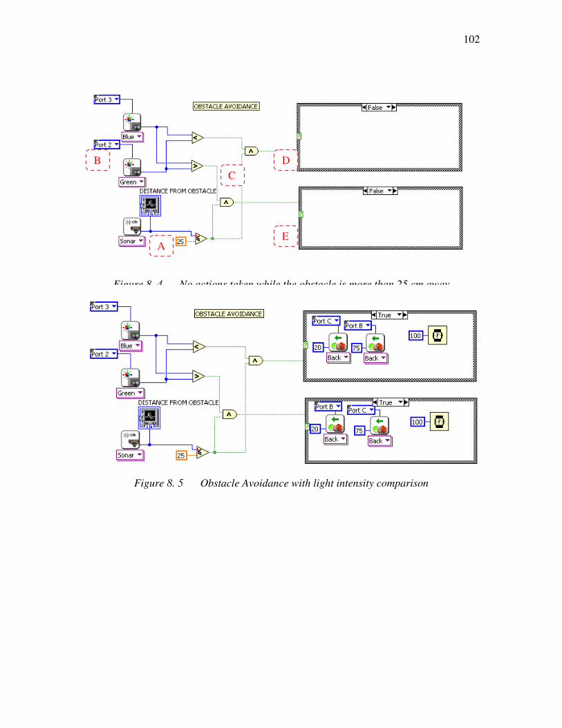
102

Figure 8. 4 No actions taken while the obstacle is more than 25 cm away

Figure 8. 5 Obstacle Avoidance with light intensity comparison

C

A

B D

E

Figure 8. 6

Simple obstacle avoidance would consist of a sonar reading to be less then a predefined

value in centimeters or inches for the robot to change its trajectory. In this case there was

another consideration taken into account as to w

provided an obstacle is detected closer than the allowable distance from the robot. For

this, the two light sensors were also taken into account.

If the distance of the robot from the obstacle is more than 25 cm, it

effect. (Fig 8.4). But as in Figure 8.5

light sensors are consulted (Label B) and the direction of backing up depends upon the

values provided by the sensors. If the right sensor exhibits h

Compare light values

between the two

sensors (Fig 5.8) (A)

Block diagram for smart obstacle avoidance



another consideration taken into account as to which direction the robot would turn


this, the two light sensors were also taken into account.

If the distance of the robot from the obstacle is more than 25 cm, it does not come into

effect. (Fig 8.4). But as in Figure 8.5, when an obstacle is detected (Label A) the two


values provided by the sensors. If the right sensor exhibits higher light value, the robot

Obstacle less than

20cm away? (B)







turning left (D)

Light value of the right


the left sensor


(Fig 5.7)

Light value of the left


the right


(Fig 5.7)

Light values of the two

sensors are equalGo straight

103



hich direction the robot would turn


s not come into

, when an obstacle is detected (Label A) the two


igher light value, the robot







turning left (D)



104 will back up facing right( Label D), and if the left light sensor is having a higher light

intensity value than the right sensor, it would back up facing to the left (Label E).

This addition to the obstacle avoidance greatly increases the efficiency of the system as

the robot not only becomes less likely to get stuck but also it reduces the navigation time

of the robot considerably to reach the goal.

In other cases the obstacle avoidance may also just be defined as backing up straight for a

set distance from an obstacle.

8.3 Fire Detection and Approach

Part of the program written for the fire detection and approach follows a simple

comparison between the two light sensors. First of all, it needs to be kept in mind that the

robot is already moving at this point in a zigzag pattern motion. As soon as one of sensors

detects an elevated value of light or heat, this part of the program comes into effect,

ending the zigzag motion pattern and starting the light following algorithm.

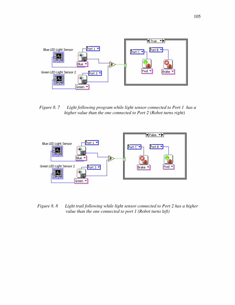
105

Figure 8. 7 Light following program while light sensor connected to Port 1 has a

higher value than the one connected to Port 2 (Robot turns right)

Figure 8. 8 Light trail following while light sensor connected to Port 2 has a higher

value than the one connected to port 1 (Robot turns left)

106

8.4 Fire Declaration

After the robot has followed the trail of light and heat and is getting closer to the fire

source, there has to be a mechanism to declare whether the approached source is fire or

not. In Chapter 6 and Chapter 7 this is described in detail because certain variables come

into play in this regard and finding the correct combination of the sensor readings to

declare a fire has to be deployed.

8.4.1 Confidence Level Definitions

The first part is to define what value has to return which confidence level, for example in

the case of two light sensors and one thermal infrared sensor, the thermal infrared sensor

is named sensor A. Numerical values are assumed plausible values to illustrate how the

approach works. If the value of A is below 60°C, there is no possibility of fire. This value

can be considered as A1, which is the fire non-possibility mode. In Chapter 7 it was

defined that at level A1, the fire is not possible no matter what values other sensors may

provide. Also a temperature value between 60°C and 100°C is considered to be the

medium confidence level, denoted by A2. Meanwhile, the temperature values between

100°C and 115°C are considered to be high confidence. Declaration of fire may happen at

these values depending upon the readings from other sensors, as that may be considered

supporting evidence for the presence of fire. Finally if the temperature reading returned

by the sensor A is above 115°C, a fire has to be present there. That level of confidence is

107 denoted as A4, and this is also called Single Sensor Declaration Mode. According to the

derivations in Chapter 7, this would be considered the declaration of fire.

An illustration of confidence levels is given in the following figure, as they were defined

in LabVIEW.

108

Figure 8. 9 Sensors and confidence levels

Figure 8.9 describes the different confidence levels as defined by the programmer. For

the TIR (Thermal Infrared Sensor), four confidence levels have been defined namely

temperature below 60° C, which is confidence level A4. This is the single sensor non-

109 possibility value as it is impossible to have a fire incident no matter what values are

returned by the light sensors. When the temperature value returned by the sensor is

between 60°C and 100°C, a medium confidence level is declared. A high confidence

value is declared between 100°C and 115°C. Medium and high confidence values are

even though not a detection mode but the possibility of fire being present there would

depend upon the “vote” and confidence levels from the other sensors in the process of

identifying a fire. The confidence level A1 is declared when temperature readings

returned by the sensor are above 115°C. At this point the software identifies the reading

as a positive identification of fire, as these temperatures are not achieved by other objects

normally.

Also the confidence levels of the two light sensors can be seen labelled as B1, B2 B3 and

C1 C2 and C3. Defining the high, medium and low confidence levels respectively for the

light sensors B and C.

Point to be noted is that the low confidence level starts at 60 Lumens. As described

previously, below 60 Lumens, the robot goes through a sinusoidal or zigzag movement

increasing its peripheral vision. When lights under 60 Lumens are detected it is not

considered to be a trail guidance signal. Hence between the light values of 60 and 90

Lumens, a low confidence is defined. Between 90 and 115 Lumens a medium confidence

level and above 115 Lumens, high confidence level is defined.

110

8.4.2 Detection Modes (Confidence Level Combinations)

As described previously a combination of confidence levels of different sensors that

declares a particular incident is called a Detection Mode. The following two scenarios

were programmed in LabVIEW for declaration of fire source

8.4.2.1 LabVIEW VI for Two Light Sensors and One TIR Sensor In the case of two light sensors and one temperature sensor, the detection modes defined

were described in Equation 7.1 as follows

This means:

If the sensor A which is the temperature sensor detects heat at the confidence level A1

(Above 115°C) OR Sensor A has a confidence level A2 AND sensor B has the

confidence level B2 OR Sensor A is at a confidence level A2 AND sensor C has the

confidence level C2 OR Sensor A has a confidence level A3 AND Sensor B has

confidence level B1 AND sensor C has confidence level C2 OR

A1 or A2B2 or A2C2 or A3B1C2 or A3B2C1 (7.1)

111

Figure 8. 10 Detection Modes in accordance to Eq. 7.1

Figure 8.10 describes the detection modes as defined in Equation 7.1. These

combinations, when obtained from the robot sensors, will be able to define a condition

that there is a fire present in a close vicinity of the robot.

L

A

B

C

E

H

F J

G

K

D

112

8.4.2.2 LabVIEW VI for One Light Sensor and Two TIR Sensors Similarly the VI (LabVIEW Virtual Instrument) for the case of two temperature sensors

and one light sensor can be created.

The Detection Modes for that case are given by equation 7.7 i.e.

The sensor arrangement also needs to be changed. As previously described the single

sensor non-possibility mode does not apply in this case as the two TIR sensors can

declare fire individually. Hence the acceptable detection modes consist of seven parts.

The LabVIEW program will need to accommodate these seven detection modes. Figure

8.9 describes the confidence levels of this sensor arrangement and the confidence levels

associated with each sensor for a particular sensor detected value.

A1 or B1 or A2B3 or A3B2 or A2C3 or B2C3 or A2B2C1 (7.7)

113

Figure 8. 11 The actual detection VI for this sensor arrangement

114

Figure 8. 12 Confidence level definition for the case of two TIR sensors and one light

sensor

115 At this point detection modes may be applied to the VI.

Figure 8. 13 Detection Modes for two TIR and one Light sensor arrangement in

accordance to eq. 7.7

Fire Declaration is a Boolean switch activated by any one of the detection modes. This

switch may start other operations such as fire extinguishing mechanism or an alarm. In

116 this VI, Motor connected to port A (also called Motor A) is one of the outputs still

available. To show the mechanism, the motor will run for one second declaring the fire.

Figure 8. 14 Open loop control of Motor A is running indicating the true condition of

the presence of fire

Figure 8. 15 Open loop control of Motor A is stopped indicating the false condition of

the presence of fire

It is to be noted that in the true condition of the presence of fire, Motor B and Motor C,

which are the driving motors are also stopped which prevents the robot to move away

from the target.

117 The complete LabVIEW Virtual Instrument or VI is the combination of all the above

mentioned conditions. The VI for the case of two light sensors and one TIR would

become:

119 Figure 8. 16 Complete LabVIEW VI for Fire Declaration algorithm with two light and

one TIR sensors. Describing Eq. 7.4

Also the final program for the scenario with two TIR sensors and one light sensor would

be as follows

Figure 8. 17 Complete LabVIEW VI for Fire Declaration algorithm with one light and

two TIR sensors in accordance with Eq. 7.7 (The other parts remain the same as figure

8.16

120

Chapter 9

Experimental Results

9.1 Introduction Experiments were performed indicating different scenarios. As described in the previous

chapters, two different sensor arrangements were used. In both the configurations, three

sensors participated in decision making process of declaration of fire and one sensor was

used for obstacle avoidance. Two different variations of algorithm were also applied to

accommodate single sensor detection mode.

In the arrangement with two light sensors and one thermal infrared sensor, the single

sensor detection mode and single sensor non possibility mode are in effect while in the

arrangement with two heat sensors and one light sensor, single sensor detection mode is

available but single sensor non-declaration is not practical as any heat sensor may declare

the presence of fire.

Experiments were performed in dimly lit environment to minimize the risk of unwanted

source seeking. While using the single sensor non declaration mode is a deterrent against

a false alarm, as the algorithm requires the heat to be present in declarations but having

multiple light sources increases the source finding time.

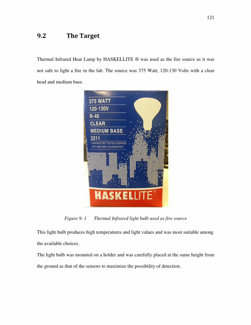
121

9.2 The Target

Thermal Infrared Heat Lamp by HASKELLITE ® was used as the fire source as it was

not safe to light a fire in the lab. The source was 375 Watt, 120-130 Volts with a clear

head and medium base.

Figure 9. 1 Thermal Infrared light bulb used as fire source

This light bulb produces high temperatures and light values and was most suitable among

the available choices.

The light bulb was mounted on a holder and was carefully placed at the same height from

the ground as that of the sensors to maximize the possibility of detection.

122

9.3 Testing Scenarios

The following scenarios were tested with both sensor arrangements

1. Target present in plain sight not directly in front of the robot

2. Target present behind a flat obstacle

3. Target present behind a set of obstacles making a concave shape

4. Target present behind a convex obstacle

5. Target present behind a flat obstacle with a reflective wall present on the side

6. Target present behind a flat obstacle with a non-reflective wall on the side

7. No target present

9.4 Sensor arrangement with two light and one

temperature sensor:

9.4.1 Target present in plain sight not directly present in front of the

robot

This is the simplest scenario where the target was in plain sight of the robot

The robot started its movement in a sinusoidal motion but as it detected elevated levels of

light it began target tracking. The following waveform charts describe the approach,

sensor readings, distance from obstacles, light values and the detection mode that was

responsible for declaration of fire incident.

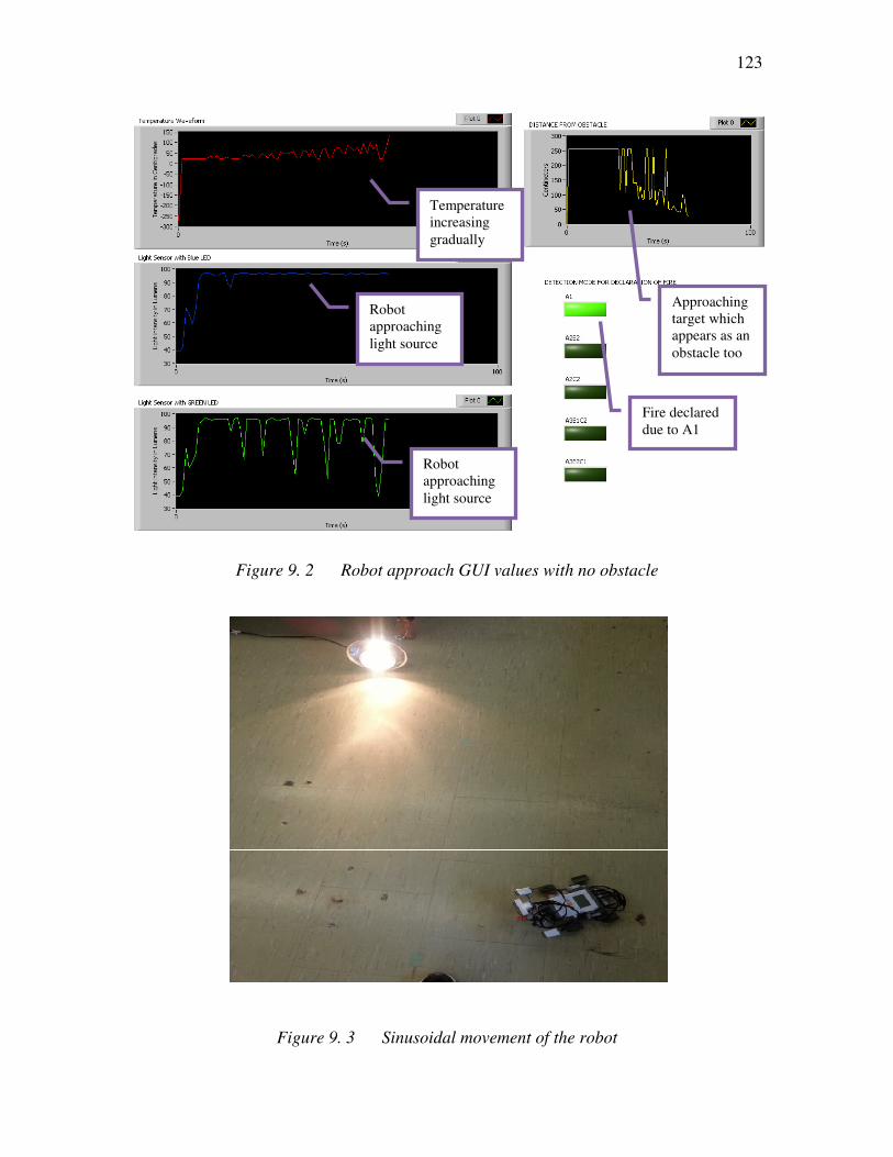
123

Figure 9. 2 Robot approach GUI values with no obstacle

Figure 9. 3 Sinusoidal movement of the robot

Temperature increasing

gradually

Approaching target which appears as an

obstacle too

Fire declared due to A1

Robot approaching

light source

Robot approaching

light source

124

Figure 9. 4 Robot detected elevated light and navigating towards it

Figure 9. 5 Robot approaching the target

125

Figure 9. 6 Sensor readings are high but the target is not declared yet

Figure 9. 7 Target declaration using modified voting logic

126 Figures 9.3 to 9.7 describe the robot motion towards the target. In Figure 9.3 Robot does

not observe the target but there is a higher value of light towards its right. The sinusoidal

movement allowed it to detect that value for the first time and then the sensor value

comparison brought it to the source. At that point, in Figure 9.7 the fire declaration

algorithm allowed the robot to positively identify the presence of fire.

At the same time the Figure 9.2 supports the movement by providing the readings for

each time. It can be clearly seen that the light values increase gradually but also a shift in

the two peak values from the two light sensors may be seen which is the guiding

mechanism of the robot. It can also be observed that the declaration of fire occurred

because of the declaration mode A1 which means that this time the sensor was directly in

front of the source and other sensors were not required to participate in the decision

making process. Meanwhile the distance to the obstacle can be observed reducing with

every cycle since the robot identifies he light bulb as an obstacle as well. Because of the

powerful light and heat combination the fire is declared in more than 24 cm which is the

minimum allowable distance of the robot with an obstacle in accordance with the

LabVIEW VI governing this source seeking.

9.4.2 Target present behind a flat obstacle

The same VI for the same sensor arrangement is used for all the experiments in this

section. In this case the target is present behind an obstacle that is flat.

127

Figure 9. 8 Target behind a flat obstacle

In this case the target was present behind a flat obstacle. It can be observed from the

temperature graph against time that the temperatures are at the room level in the first ten

seconds but the light values differ. That leads the robot to move and follow the light.

Once the source is detected it can be observed that whenever the robot goes behind an

obstacle, the temperature values fall to the room temperature. Also when there is no

obstacle in sight the Sonar sensor returns the value of 255cm for the distance hence the

graph never goes over 255 for the proximity sensor.

Temp. gradually

increasing

Its colder behind an obstacle

Obstacle cleared and elevated temperatures

are detected

Obstacle

approach

Obstacle cleared, approaching target

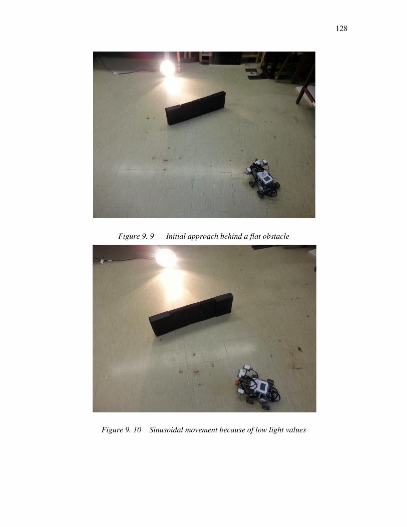
128

Figure 9. 9 Initial approach behind a flat obstacle

Figure 9. 10 Sinusoidal movement because of low light values

129

Figure 9. 11 Going around the obstacle

Figure 9. 12 Clearing the obstacle

130

Figure 9. 13 Target approach

Figure 9. 14 Target (Source) declaration with detection mode A2B2

131

It was also observed that when the robot crosses the obstacle from the right side, it tends

to touch and sometimes knock over the obstacle. Even though it does not affect the

working of the robot, it is not desirable. To overcome this challenge, the backing up time

was increased to 1 second (1000 ms) with results

9.4.3 Target present behind a concave obstacle

Figure 9. 15 Target present behind a concave obstacle

It was observed that while approaching the source with concave shaped obstacles, the

directional backing up was not successful and the robot got stuck 3 times out of 10.

132 The VI was modified slightly to allow the robot to back up straight for 1 second and

restart the approach towards the target. This allowed the robot enough time to get out of

the concave obstacle and find the light or heat signal to follow.

Figure 9. 16 Concave obstacle target detected with detection mode A1

Robot approaching light source

Robot approaching

light source

Concave

Obstacle

Obstacle cleared, robot

moving to the target

Temperature exceeds the declaration limit

Fire declared

due to A1

Fluctuation of readings due to

comparative sensor approach

133

9.4.4 Target present behind a convex obstacle Finding a target behind a convex obstacle was the easiest of all the scenarios.

Figure 9. 17 Target behind a convex obstacle

134

Figure 9. 18 Target declaration behind a convex obstacle with two detection modes

Robot approaching light source in a sensor comparison approach

Robot approaching

light source

Obstacle

cleared easily

Fire declaration due to two

detection modes

135

Figure 9. 19 Another case with different detection mode for target present behind a

convex obstacle

9.4.5 Target present behind a flat obstacle with a reflective wall on

one side

This is one of the most interesting results. Looking at the graphs closely it can be

observed that elevated temperatures and light values were detected starting the timeslot of

46 seconds. Then the temperature and light values abruptly come to a lower level. At that

point there is a little sinusoidal-like variation in the light intensity values and

temperatures. Then the values increase and the robot follows a familiar approach until

declaration of the fire, which, in this case, happens to be a single sensor declaration mode

identified as A1.

Obstacle

Target

Fire declaration due to A1 (Straight

approach)

Robot approaching

light source

Robot approaching

light source

Declaration

136

In this particular case the robot started its approach towards the wall after the detection of

elevated light values, as the wall was reflecting light. As the robot approached the wall

the obstacle avoidance mechanism kicked in. In the obstacle avoidance as there is

gradient of light comparison also included, therefore the robot faced the source while

backing up. Right from there, the case practically becomes as described in the first

scenario, i.e. the source in plain sight of the robot.

Figure 9. 20 Flat obstacle with a reflective wall

137

Figure 9. 21 Robot follows the reflected light from the obstacle

Figure 9. 22 Robot approaches the reflected light from the obstacle

138

Figure 9. 23 Robot detects higher values of light and temperature as it turns back

facing towards a higher value of light

Figure 9. 24 Robot clears the obstacle and is following the correct source

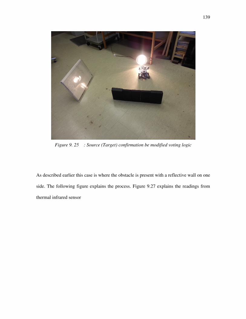
139

Figure 9. 25 : Source (Target) confirmation be modified voting logic

As described earlier this case is where the obstacle is present with a reflective wall on one

side. The following figure explains the process. Figure 9.27 explains the readings from

thermal infrared sensor

140

Figure 9. 26 An explanation of the thermal readings and milestones

If the Sonar waveform is closely examined in the following figure it can be clearly seen

that the robot follows the reflected light, detects reflected wall as an obstacle, which is

where its reading dips down to a lower value. Again the lower values are seen because of

the actual obstacle as it passes by it. While it performs obstacle avoidance it faces the

actual source of light and heat and follows it to declare a fire incident.

Following reflected heat off the wall

The wall itself is not hot

Crossed the obstacle and reflective wall

Declared the fire because of temperatures exceeding predefined limits

autonomous fire detection robot using modified voting … · autonomous fire detection robot using...

Documents