autopipe training outline
DESCRIPTION
training materialTRANSCRIPT
Bentley Confidential 1
AutoPIPE Advanced Training Outline
Component Modeling • Nozzle/Vessel models in AutoPIPE • Nozzle/Vessel Stresses Using WINNOZL • Expansion Joints • Jacketed Piping • Valves • Reducers • Flanged elbows, miters and bends • Tees • Frame
Nonlinear Analysis
• Analysis assumptions (linear and non-linear) • Support non-linearity’s • Load sequencing • Non-linear occasional loads • Result interpretation
Dynamics
• Analysis assumptions • Analysis algorithms • Frequency and Mode Shapes • Response spectrum analysis • Spectrum Enveloping • Static Correction • Harmonic analysis • Force spectrum analysis • Seismic Anchor Movement Analysis • Time history analysis • Dynamic Load Factor
Fluid Transients • Water hammer analysis • Steam relief valve analysis • Slug flow analysis
Miscellaneous • Buried pipe analysis • Submerged piping and wave loads • Special Modeling Cases • Open discussion

Bentley Confidential 2
Vessel and Nozzle Modeling Considerations
• Nozzles of equipment like pump and compressors are modeled as Anchor
• Vessel nozzle can be generally modeled as Anchors - May give too
conservative values for forces on equipment nozzle • Nozzle option allows modeling of local stiffness effects of the vessel
and nozzle junction • Commonly used methods of calculating nozzle stiffness
• Finite element modeling • ASME III Class I - implemented in AutoPIPE • API 650 - implemented in AutoPIPE • Bijllard theory - implemented in AutoPIPE • Welding Research Council Bulletin 297 - based on Steele’s
theory - implemented in AutoPIPE
• Other than finite element model, all methods are approximate and only valid for a specified range of nozzles. Finite element method will take longer time and is impractical for everyday design.
• Nozzle option only models the local effects of nozzle and vessel. The vessel must be modeled separately.
• Nozzle may be connected to a Cylindrical or Spherical vessels. Nozzle connected to cylindrical vessel is more sensitive to diameter of the pipe.
• AutoPIPE uses flexible joint element to model a nozzle
• Unbalanced pressure thrust effect is not modeled. Please refer to WinNOZL WRC368 and applied radial load.
Bentley Confidential 3
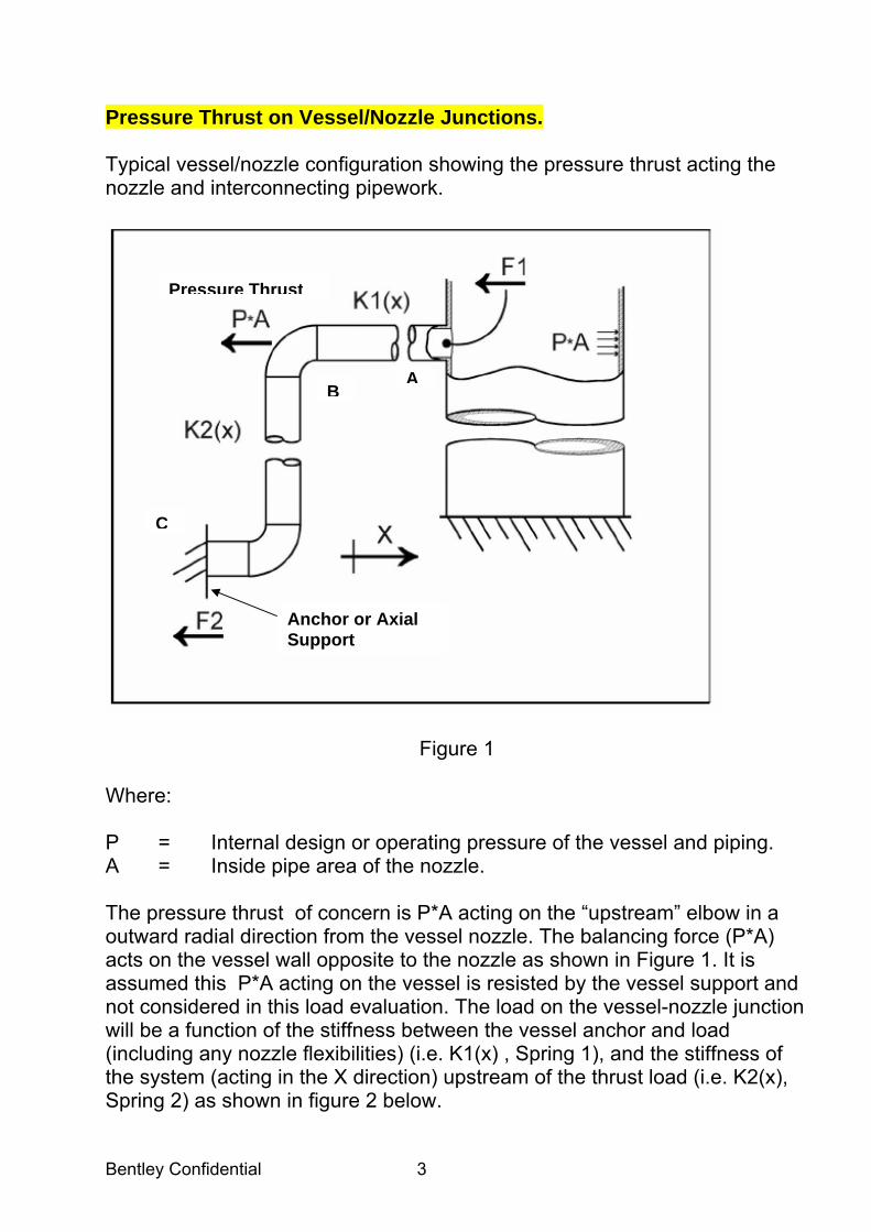
Pressure Thrust on Vessel/Nozzle Junctions. Typical vessel/nozzle configuration showing the pressure thrust acting the nozzle and interconnecting pipework.
Figure 1 Where: P = Internal design or operating pressure of the vessel and piping. A = Inside pipe area of the nozzle. The pressure thrust of concern is P*A acting on the “upstream” elbow in a outward radial direction from the vessel nozzle. The balancing force (P*A) acts on the vessel wall opposite to the nozzle as shown in Figure 1. It is assumed this P*A acting on the vessel is resisted by the vessel support and not considered in this load evaluation. The load on the vessel-nozzle junction will be a function of the stiffness between the vessel anchor and load (including any nozzle flexibilities) (i.e. K1(x) , Spring 1), and the stiffness of the system (acting in the X direction) upstream of the thrust load (i.e. K2(x), Spring 2) as shown in figure 2 below.
Anchor or Axial Support
Pressure Thrust
AB
C

Bentley Confidential 4
Figure 2
The force F is in equilibrium with the two spring forces F1 and F2: F = F1 + F2 (1) The spring stiffness K and the displacement δ can be related as: K1 = F1 / δ1 K2 = F2 / δ2 So: F = δ1 * K1 + δ2 * K2 Since, δ1 = δ2, let’s denote it by δ: So: F = δ * ( K1 + K2 ) δ = F / ( K1 + K2 ) Pressure thrust load on the vessel-nozzle junction: F1 = F * K1 / ( K1 + K2 ) (2) If the piping system on the other side of the applied load (Spring 2) is stiff, for example due to an anchor, then pressure thrust will be absorbed by the anchor. Thus, the nozzle will experience very little direct axial stress. This can be seen from equation 2. Note that a greater K2 results in a lower thrust force F1. Therefore, in this case including all of the pressure thrust into analysis will be conservative. However if the pipe shown by spring 2 is flexible (maybe an expansion loop or small diameter pipe with bends) then the nozzle will see more of the force due to the pressure thrust. Therefore it is appropriate to analyze the local vessel/nozzle stresses due to most of the pressure thrust load.
Pressure Thrust (P*A)

Bentley Confidential 5
Pressure Thrust Guidelines If the combined (membrane + bending) stresses exceed the allowable stress with the applied full (pressure thrust option under combinations Load TAB) or partial (applied load with correct sign under LOADS TAB) thrust load then it is suggested to check the membrane and combined (secondary ) stress levels with WRC368 option enabled and thrust load (or option) removed. WinNOZL WRC368 within its geometric limits provides a good design check of pressure stress levels which includes the full thrust load otherwise use FEA analysis to obtain more accurate combined stresses. If the full pressure thrust is acting on the vessel/nozzle junction e.g. nozzle with a blind flange then FEA would generally be the most accurate analysis tool to evaluate. Note: FEA programs have limitations due to the accuracy of the type of elements used e.g. many programs use thin shell elements which do not capture transverse shear effects of thick shell elements.
Bentley Confidential 6
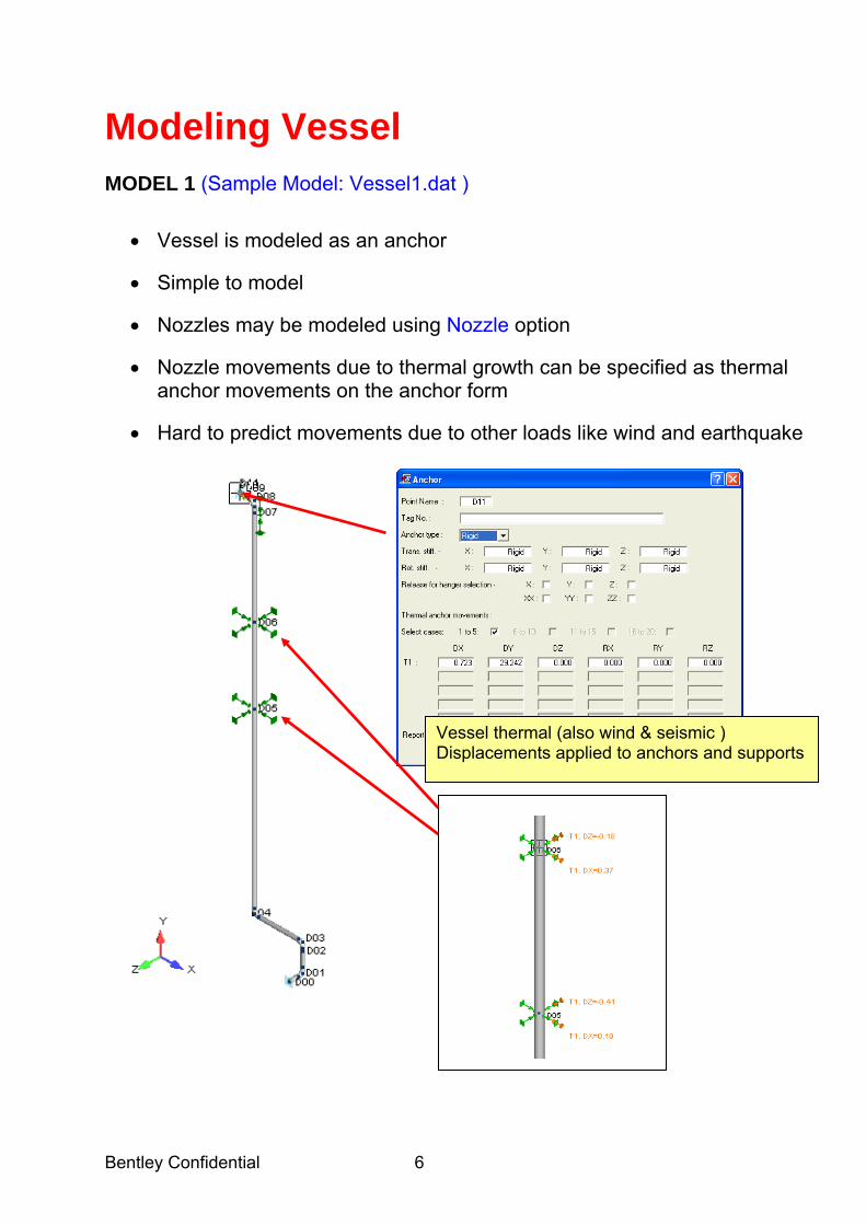
Modeling Vessel MODEL 1 (Sample Model: Vessel1.dat )
• Vessel is modeled as an anchor
• Simple to model
• Nozzles may be modeled using Nozzle option
• Nozzle movements due to thermal growth can be specified as thermal anchor movements on the anchor form
• Hard to predict movements due to other loads like wind and earthquake
Vessel thermal (also wind & seismic ) Displacements applied to anchors and supports
Bentley Confidential 7
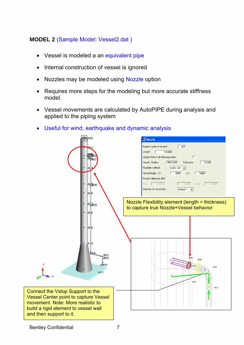
MODEL 2 (Sample Model: Vessel2.dat )
• Vessel is modeled a an equivalent pipe
• Internal construction of vessel is ignored
• Nozzles may be modeled using Nozzle option
• Requires more steps for the modeling but more accurate stiffness model.
• Vessel movements are calculated by AutoPIPE during analysis and applied to the piping system
• Useful for wind, earthquake and dynamic analysis
Connect the Vstop Support to the Vessel Center point to capture Vessel movement. Note: More realistic to build a rigid element to vessel wall and then support to it.
Nozzle Flexibility element (length = thickness) to capture true Nozzle+Vessel behavior

Bentley Confidential 8
Nozzle Stresses Using WinNOZL
• Including shell flexibility in AutoPIPE model
• Proper nozzle length to use in AutoPIPE
• Modeling pressure thrust and nozzle thermal/pressure movements. WRC368 method recommended to check pressure thrust design.
• Estimating nozzle loads in AutoPIPE
• Exporting nozzle loads into WINNOZL
• Peak stress calculation • API 650: Tanks (large diameter cylindrical shells)
• WRC 107 and PD5500: Cylindrical and Spherical shells
• WRC297: Addendum to WRC 107 for cylindrical shells. More
accurate and gives stresses in the nozzle in addition to nozzle-
shell and pad-shell junction stresses
• KHK level 1 and 2
• Peak stress evaluation using ASME Section VIII, Division 1 or Division
2 and PD5500.
• Pad design and allowable loads
Bentley Confidential 9
Expansion Joints
• Used to absorb thermal expansion to reduce movement of pipe at equipment
• Types of expansion joints:
• Bellows (tied and untied) • Universal expansion joint • Pressure balanced expansion joint • Hinged expansion joint • Gimbal • Slip Joint • Ball Joint
• Modeled using Flexible Joint • Ability to specify axial, shear, torsional and bending rates • Torsion may be modeled as rigid or free • Back-to-back flexible joint may cause instability if not modeled
properly.
• Internal pressure causes bellows to expand. Must be constrained using external supports or tie rods.
• Tie rods can be modeled using tie link. This is a simplified model
and does not capture bending resistance due to locking of rods • The bending moment resistance of tie rods can be captured using a
comprehensive model of tie rod assembly using beams. The modeling is complex and not always necessary for design.
Bentley Confidential 10
Jacketed Piping • Carrier pipe and jacket modeled as two separate segments with
different pipe identifiers e.g. Jacket6 and carrier8
• Segments may be made of different materials and have different operating conditions
• Carrier pipe is supported by the jacket at regular intervals using spacers and at flanged ends.
• Spacers are modeled as two point supports e.g. guide between a carrier segment point and a jacket segment point with same coords.
• Flanged ends can be modeled in two different ways. For purposes of structural analysis, both models are same
• If both carrier and jacket are liquid filled then adjust jacket SG.
• Remember to only apply hydrodynamic (e.g. submerged piping), wind and insulation only to jacket.
• Ideally suited for graphical copy/paste operations
• New segment cannot be inserted at the start of a 2 point component like a valve. New segment at end of the valve is ok therefore need to insert small run point before the valve to connect the jacket segment.

Bentley Confidential 11
MODEL 1 – Beam connected model (Sample model: jacket1.dat)
• Flanged ends are modeled as rigid beams between a point on the carrier segment and the jacket segment
• Model is applicable for all types of flanged ends
STEPS
1. Open Jacket_1A
2. View/Transparency : Pipe = checked
3. Select range C02 to C12, and also branch B16 to B04 so highlighted red.
4. Edit /copy using base point = C02

Bentley Confidential 12
5. Select / Clear
6. Click cursor on point C02 (so point name = RED) and Edit/Paste , uncheck the “connect to select points” then click Ok (This creates jacket segments D and E)
7. View / segment and uncheck all segments except D & E
8. Select / All or Select /Segment to select segments D & E
9. Edit/ Move/Stretch , Enter DY = 0.01 10. Select / Clear 11. Select Segment E and Modify/Pipe properties over Range, and select
pipe identifier = Jacket8 12. Select / Clear 13. Select Segment D and Modify/Pipe properties over Range, and select
pipe identifier = Jacket6

Bentley Confidential 13
14. Click on point E07 (previously a reducer on carrier pipe) and
Modify/convert point to run 15. Delete the additional flanges at C02, D00 and E10, Select / Flanges,
Press Delete key Now connect Jacket to the Carrier 16. View/Show All components 17. Click on point E00 and Insert / Frame , enter J point = C02, Table name
= RIGID. 18. Click on point D00 and Insert / Frame , enter J point = B04, Table name
= RIGID. 19. Click on point E10 and Insert / Frame , enter J point = C12, Table name
= RIGID. The Jacket is now connected to the carrier at C02, B04 and C12 using rigid beams.
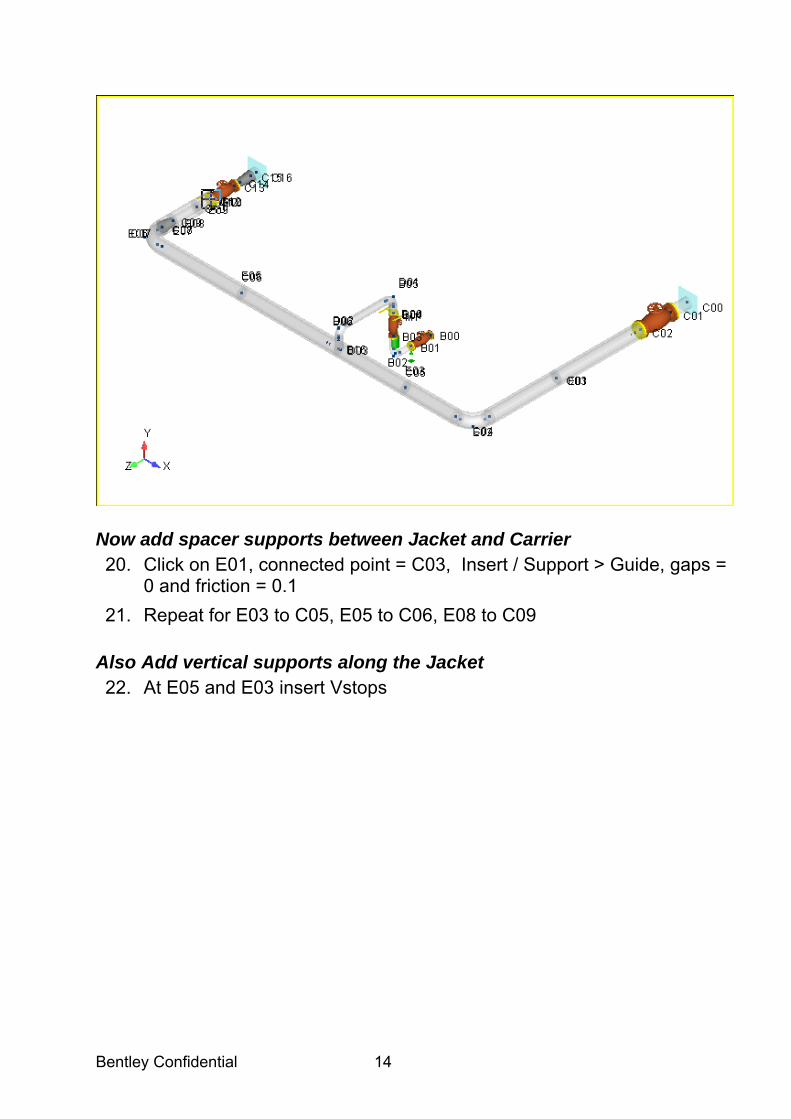
Bentley Confidential 14
Now add spacer supports between Jacket and Carrier 20. Click on E01, connected point = C03, Insert / Support > Guide, gaps =
0 and friction = 0.1 21. Repeat for E03 to C05, E05 to C06, E08 to C09
Also Add vertical supports along the Jacket 22. At E05 and E03 insert Vstops
Bentley Confidential 15
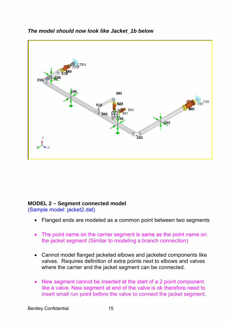
The model should now look like Jacket_1b below
MODEL 2 – Segment connected model (Sample model: jacket2.dat)
• Flanged ends are modeled as a common point between two segments
• The point name on the carrier segment is same as the point name on the jacket segment (Similar to modeling a branch connection)
• Cannot model flanged jacketed elbows and jacketed components like valves. Requires definition of extra points next to elbows and valves where the carrier and the jacket segment can be connected.
• New segment cannot be inserted at the start of a 2 point component like a valve. New segment at end of the valve is ok therefore need to insert small run point before the valve to connect the jacket segment.
Bentley Confidential 16
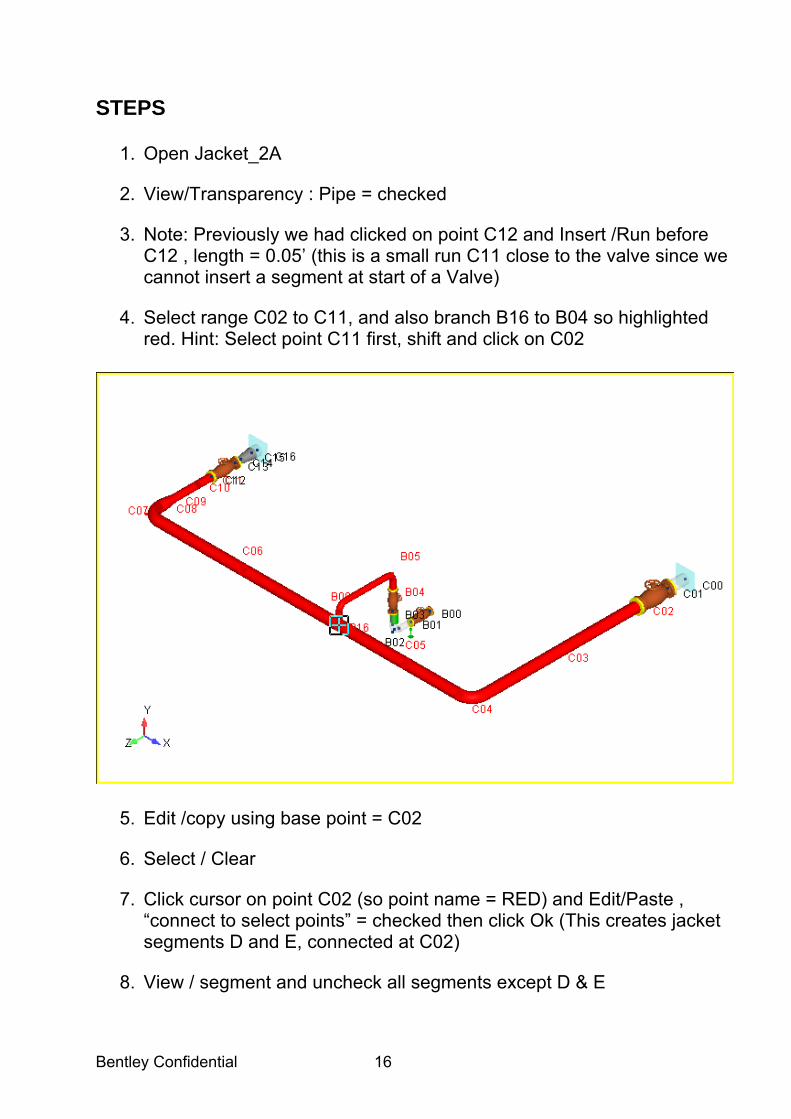
STEPS
1. Open Jacket_2A
2. View/Transparency : Pipe = checked
3. Note: Previously we had clicked on point C12 and Insert /Run before C12 , length = 0.05’ (this is a small run C11 close to the valve since we cannot insert a segment at start of a Valve)
4. Select range C02 to C11, and also branch B16 to B04 so highlighted red. Hint: Select point C11 first, shift and click on C02
5. Edit /copy using base point = C02
6. Select / Clear
7. Click cursor on point C02 (so point name = RED) and Edit/Paste , “connect to select points” = checked then click Ok (This creates jacket segments D and E, connected at C02)
8. View / segment and uncheck all segments except D & E
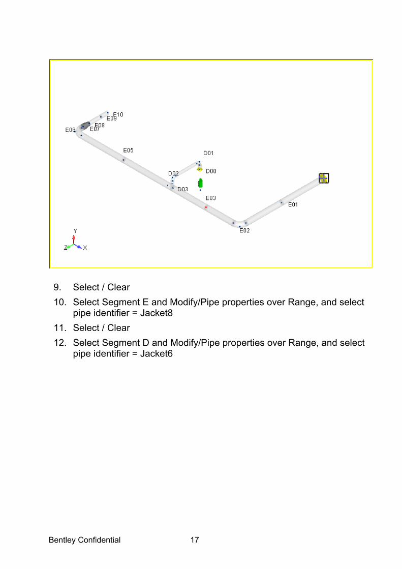
Bentley Confidential 17
9. Select / Clear 10. Select Segment E and Modify/Pipe properties over Range, and select
pipe identifier = Jacket8 11. Select / Clear 12. Select Segment D and Modify/Pipe properties over Range, and select
pipe identifier = Jacket6
Bentley Confidential 18
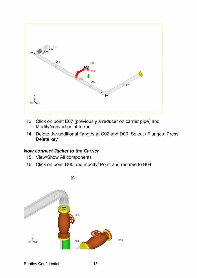
13. Click on point E07 (previously a reducer on carrier pipe) and
Modify/convert point to run 14. Delete the additional flanges at C02 and D00 Select / Flanges, Press
Delete key Now connect Jacket to the Carrier 15. View/Show All components 16. Click on point D00 and modify/ Point and rename to B04

Bentley Confidential 19
17. Similarly click on point E10 (or F5 goto point) and modify/ Point and
rename to C11 The Jacket is now connected to the carrier at C02, B04 and C11 using tee segment connections
Now change all the Welding tees at C02, B04 and C11 to Tee type = Other with SIF = 1.0. 18. This can easily be done in the Tee Input Grid using multiple Select of
“Type “ cell and use CTRL key to change to OTHER and then press CTRL + Enter
Now add spacer supports between Jacket and Carrier 19. Click on E01, connected point = C03, Insert / Support > Guide, gaps =
0 and friction = 0.1 20. Repeat for E03 to C05, E05 to C06, E08 to C09
Also Add vertical supports along the Jacket 21. At E05 and E03 insert Vstops
Bentley Confidential 20
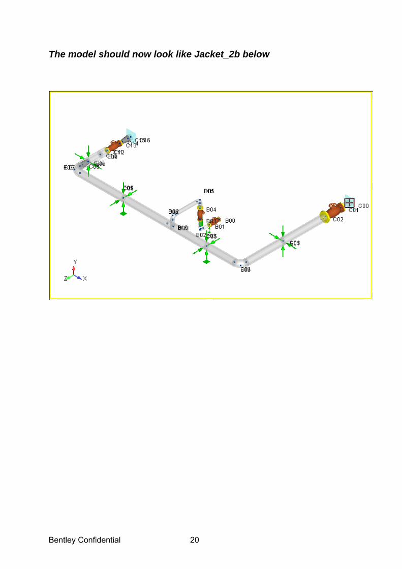
The model should now look like Jacket_2b below
Bentley Confidential 21
Valves
• Construction of valves makes it stiffer than pipe. The stiffness of valve cannot be estimated without a detailed finite element analysis of the valve.
• For purposes of piping design, valves are modeled as stiff pipes
• AutoPIPE models a valve as 100 times stiffer than the pipe at starting point of the valve. This is achieved by increasing the modulus of elasticity of the pipe.
• Specified weight of the valve is distributed evenly along the length
ANGLE VALVES
• Angle valves and Relief valve can be modeled using valve component and specifying offsets of the far end from the valve point
• The valve is defined as a tilted valve. The exact form of the valve is not important as long as end points are defined at correct location
• AutoPIPE will generate a warning during global consistency check
VALVE OPERATORS
• Heavy operator far from valve center of gravity can induce significant force into the piping system in seismic event.
• Eccentric weight can be used to model operators
• This model is accurate for static loads including earthquake cases. Ignores off diagonal mass matrix terms. May not be exact if operator weight is large compared to valve weight
• Exact model of the operator requires a rigid beam with weight at the free end. Modeling is complex and may not be necessary

Bentley Confidential 22
Reducers
• Used at locations where pipe size changes
• AutoPIPE generates a warning if pipe size is changed without using a reducer component
• Eccentric reducers are modeled by specifying offset of the far end
• Cone angle of the reducer (for SIF) is calculated based on the full length of the reducer.
• For analysis purposes, a reducer is modeled as a pipe with average diameter, thickness and weight per unit length.
• This model captures the exact axial behavior. The bending behavior is approximate
Bentley Confidential 23
Bends and Elbows
• Elbows tend to become more flexible with increase in plane bending due to ovaling – Von Karman effect
• The change in section modulus due to ovaling is not considered
• Ovaling also changes stress distribution and maximum stress
• Internal pressure also stiffens the elbow. The change is not significant for most operating pressure ranges.
• Flexibility factors and Stress Intensification Factors (SIF's) are used capture effects due to ovaling
• Flanged elbows are stiffer than regular elbows
• ASME codes require different flexibility factor for elbows flanged at one and both ends
• Increases SIF factors at the elbow
• AutoPIPE uses curved pipe element to model a bend
• Miters are modeled as bends with modified flexibility factors and SIF's
• Special bend components can be modeled as bends with user specified flexibility factor and SIF’s
Bentley Confidential 24
Tees
• Tee component is modeled as single point connecting, three pipes • End points of a tee components are not modeled and the change in
thickness/diameter is ignored • Tees information is only used to determine SIF at the branch
connection per piping code. • SIF's are used to capture local stresses at the branch-header junction
and their affect on strength due to cyclic thermal loading. • Some codes (B31.3) do not provide any guidelines for use of SIF's at
tees for sustained loading and occasional loading • SIF's for tees are empirical based on fatigue test a series of simple full
size tees. SIF's for other types of tees (reduced) are derived from this study.
• Piping codes do not specify SIF's for connections like laterals, Y's and
crosses. User must specify SIF's for code compliance. Bonney forge does provide a published technical paper on calculating SIF’s for lateralets.
Bentley Confidential 25
FRAMES
• To model racks and pipe supports • Usually modeled as rigid supports • Useful in dynamic analysis to capture pipe / structural interaction.
Options
• Add • Delete • Modify
Features
• Beta angle • AISC cross section & material library • Rigid lengths • End releases

Bentley Confidential 26
Analysis Assumptions
• Finite element Analysis (stiffness method) • Beam element - Uses center line dimensions • Elastic response - small deformation theory (1st order only). e.g. One
rule of thumb: Check that the maximum slope angle in radians of the deformed pipe = approx. sin(slope angle) then the solution should be ok.
• Pipes remain linear - no yielding of pipe • Supports may act one way or both ways • Longitudinal bending deformations only. Ignore local stress like
bending of pipe wall and stress concentration at tees and bends (SIF's are used to capture this behavior). Use FE or WRC local stress program like WinNOZL.
• Six degrees of freedom per node • Analysis is performed by solving a set of linear equations
[K] [U] = [R] where, K = structural stiffness matrix U = response (displacement) matrix R = applied load matrix • Gauss elimination method for solution of these equations
Bentley Confidential 27
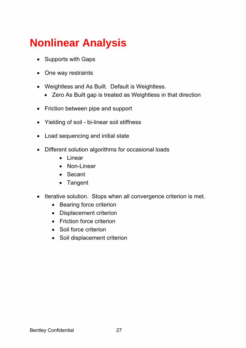
Nonlinear Analysis
• Supports with Gaps • One way restraints • Weightless and As Built. Default is Weightless.
• Zero As Built gap is treated as Weightless in that direction
• Friction between pipe and support • Yielding of soil - bi-linear soil stiffness • Load sequencing and initial state • Different solution algorithms for occasional loads
• Linear • Non-Linear • Secant • Tangent
• Iterative solution. Stops when all convergence criterion is met.
• Bearing force criterion • Displacement criterion • Friction force criterion • Soil force criterion • Soil displacement criterion

Bentley Confidential 28
Load Sequencing & Interpretation
• A load case (e.g. gravity, thermal, wind, etc.) represents an increment of load, NOT a total load (except for gravity) for linear or non-linear analysis.
• Combinations (or "Superposition" of load cases) must be defined to obtain total load effects which is a commonly accepted principle for a static linear analysis.
• Load sequencing is required in non-linear analysis
• Principal of superposition does not apply in non-linear analysis, therefore the starting point for a load case is important.
e.g. The results for Thermal load case will depend on state of supports (gaps) at the end of Gravity analysis. Some gaps may be open, other may be closed.
• Default load sequencing
• GR is analyzed with no initial state • Thermal load cases are analyzed with GR as the initial load case • Pressure load cases are analyzed with the corresponding thermal
(T?) load case as the initial load case • Occasional load cases are analyzed with GR as the initial load case
• Operating condition is determined by combining Gravity load case and thermal load case
• The end state of the piping system is always the same i.e. Operating case GR + T1 + P1 results are the same if use load sequence Gr -> T1 -> P1 or Gr -> P1 -> T1
Bentley Confidential 29
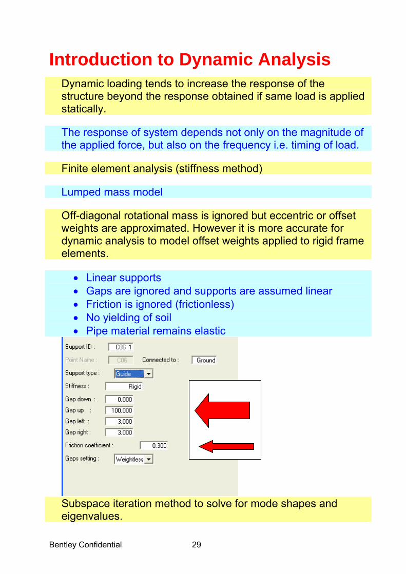
Introduction to Dynamic Analysis
Dynamic loading tends to increase the response of the structure beyond the response obtained if same load is applied statically. The response of system depends not only on the magnitude of the applied force, but also on the frequency i.e. timing of load. Finite element analysis (stiffness method) Lumped mass model Off-diagonal rotational mass is ignored but eccentric or offset weights are approximated. However it is more accurate for dynamic analysis to model offset weights applied to rigid frame elements.
• Linear supports • Gaps are ignored and supports are assumed linear • Friction is ignored (frictionless) • No yielding of soil • Pipe material remains elastic
Subspace iteration method to solve for mode shapes and eigenvalues.

Bentley Confidential 30
Static correction can be used to capture effect of mass not captured by eigenvalue analysis
• Missing Mass Correction • Zero Period Acceleration (ZPA)
Mass distribution of the model can be controlled by the user. Recommend always set Tools / model options / Edit , “Mass points per span” = A , to allow the program to capture the mass in the piping system. Forces and moments are always positive Accelerations are reported by AutoPIPE for pipe and now frame points which is an important criteria. E.g. valves in a nuclear power plant, must be able to resist 4g & 5g for OBE & SSE loadings, respectively. A common rule of thumb is to capture at least 75% of the modal mass Types of Dynamic Analyses include: Response Spectrum, Harmonic, Force Spectrum, SAM and Time History. In cases where the dynamic load is applied very near a support or directly at the support, the support reaction may be near zero or very much less than the actual reaction. The reason is because the mode shapes involving the movement between the applied load direction and the support point were not computed as specified by the number of modes or cut-off frequency. These missing mode shapes are usually very stiff and hence associated with mode shapes in the high frequency range. In such cases, an additional static earthquake analysis should be performed and the maximum reaction from both static and dynamic analyses should be used. This can be easily done by using the ZPA option which envelops dynamic results with equivalent static results.
Bentley Confidential 31
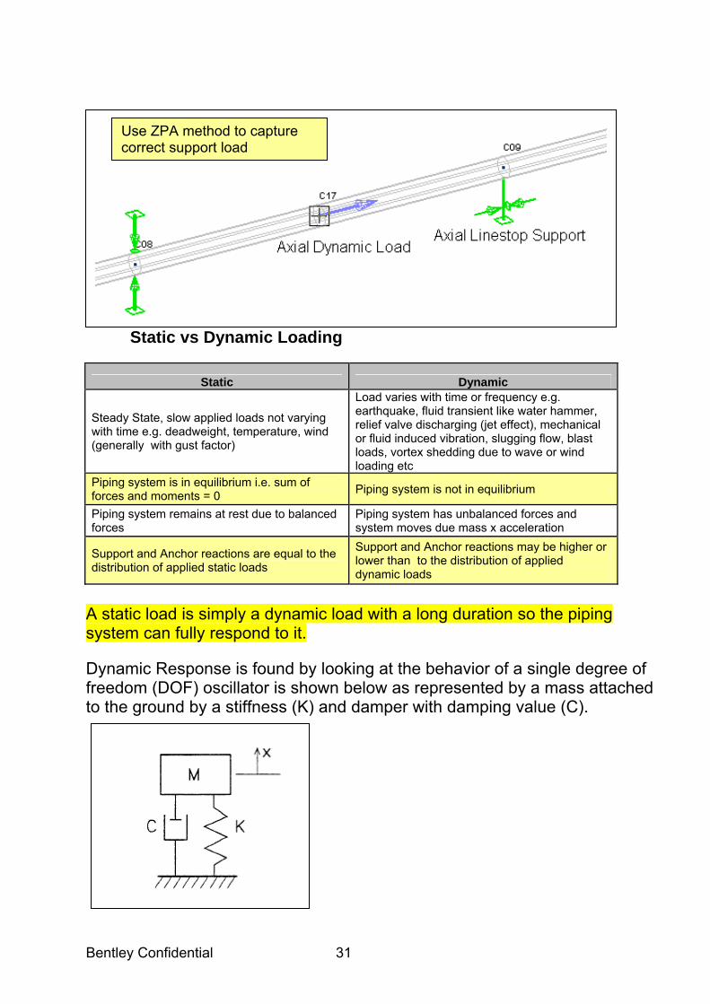
Static vs Dynamic Loading
Static Dynamic
Steady State, slow applied loads not varying with time e.g. deadweight, temperature, wind (generally with gust factor)
Load varies with time or frequency e.g. earthquake, fluid transient like water hammer, relief valve discharging (jet effect), mechanical or fluid induced vibration, slugging flow, blast loads, vortex shedding due to wave or wind loading etc
Piping system is in equilibrium i.e. sum of forces and moments = 0 Piping system is not in equilibrium
Piping system remains at rest due to balanced forces
Piping system has unbalanced forces and system moves due mass x acceleration
Support and Anchor reactions are equal to the distribution of applied static loads
Support and Anchor reactions may be higher or lower than to the distribution of applied dynamic loads
A static load is simply a dynamic load with a long duration so the piping system can fully respond to it. Dynamic Response is found by looking at the behavior of a single degree of freedom (DOF) oscillator is shown below as represented by a mass attached to the ground by a stiffness (K) and damper with damping value (C).
Use ZPA method to capture correct support load
Bentley Confidential 32
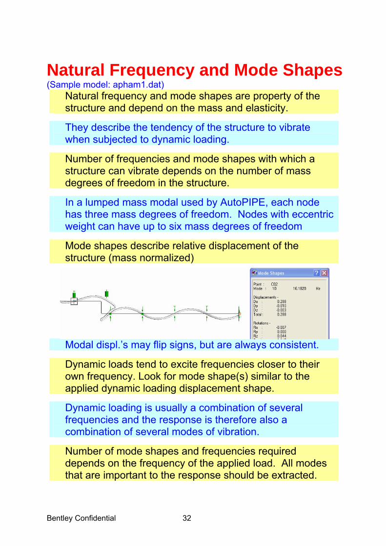
Natural Frequency and Mode Shapes (Sample model: apham1.dat)
Natural frequency and mode shapes are property of the structure and depend on the mass and elasticity.
They describe the tendency of the structure to vibrate when subjected to dynamic loading.
Number of frequencies and mode shapes with which a structure can vibrate depends on the number of mass degrees of freedom in the structure.
In a lumped mass modal used by AutoPIPE, each node has three mass degrees of freedom. Nodes with eccentric weight can have up to six mass degrees of freedom
Mode shapes describe relative displacement of the structure (mass normalized)
Modal displ.’s may flip signs, but are always consistent.
Dynamic loads tend to excite frequencies closer to their own frequency. Look for mode shape(s) similar to the applied dynamic loading displacement shape.
Dynamic loading is usually a combination of several frequencies and the response is therefore also a combination of several modes of vibration.
Number of mode shapes and frequencies required depends on the frequency of the applied load. All modes that are important to the response should be extracted.
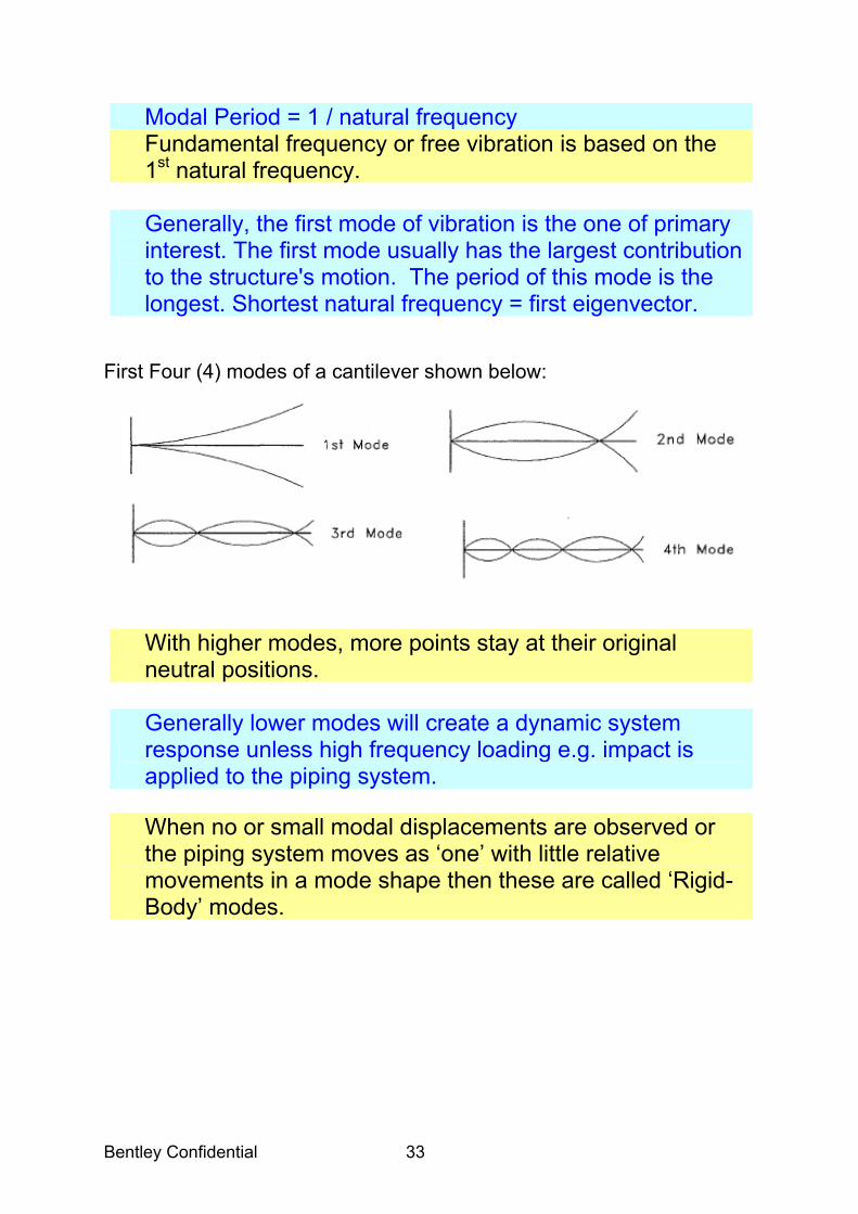
Bentley Confidential 33
Modal Period = 1 / natural frequency Fundamental frequency or free vibration is based on the 1st natural frequency. Generally, the first mode of vibration is the one of primary interest. The first mode usually has the largest contribution to the structure's motion. The period of this mode is the longest. Shortest natural frequency = first eigenvector.
First Four (4) modes of a cantilever shown below:
With higher modes, more points stay at their original neutral positions. Generally lower modes will create a dynamic system response unless high frequency loading e.g. impact is applied to the piping system.
When no or small modal displacements are observed or the piping system moves as ‘one’ with little relative movements in a mode shape then these are called ‘Rigid-Body’ modes.
Bentley Confidential 34
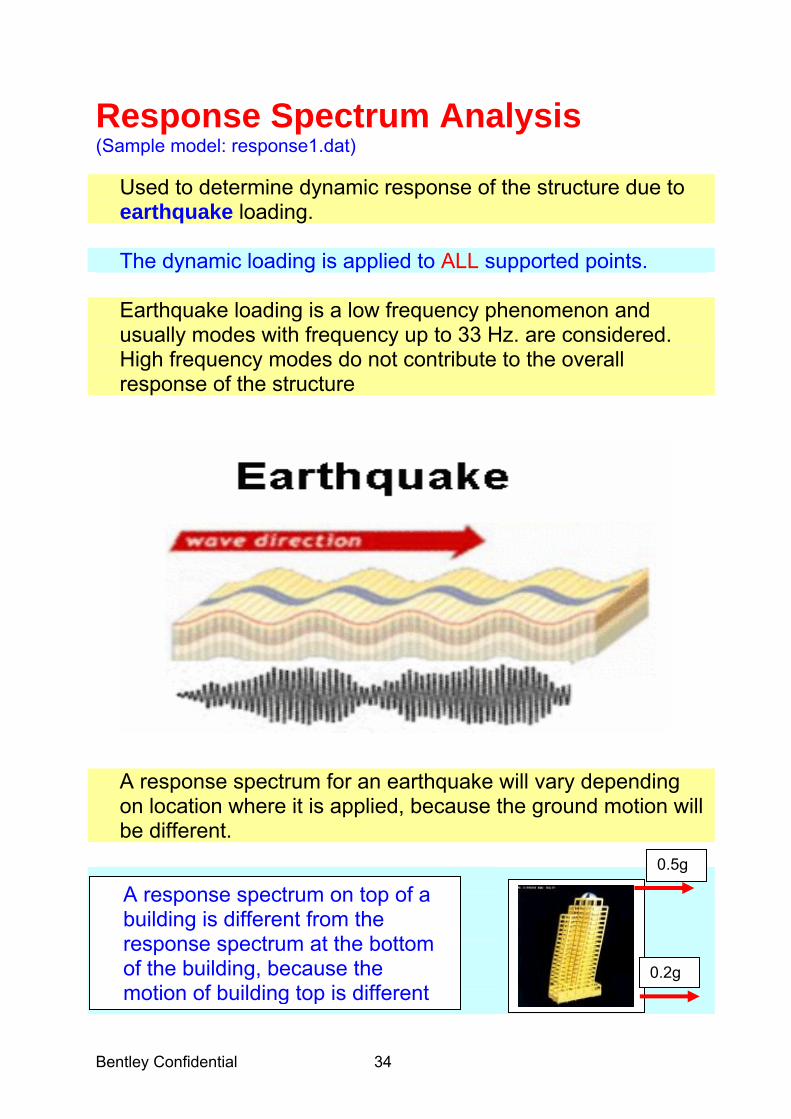
Response Spectrum Analysis (Sample model: response1.dat)
Used to determine dynamic response of the structure due to earthquake loading. The dynamic loading is applied to ALL supported points. Earthquake loading is a low frequency phenomenon and usually modes with frequency up to 33 Hz. are considered. High frequency modes do not contribute to the overall response of the structure
A response spectrum for an earthquake will vary depending on location where it is applied, because the ground motion will be different.
A response spectrum on top of a building is different from the response spectrum at the bottom of the building, because the motion of building top is different
0.5g
0.2g
Bentley Confidential 35
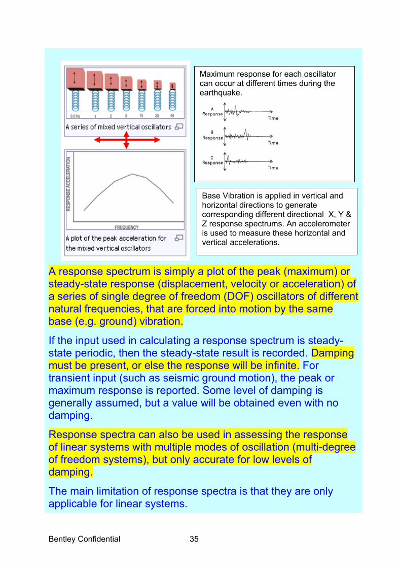
A response spectrum is simply a plot of the peak (maximum) or steady-state response (displacement, velocity or acceleration) of a series of single degree of freedom (DOF) oscillators of different natural frequencies, that are forced into motion by the same base (e.g. ground) vibration.
If the input used in calculating a response spectrum is steady-state periodic, then the steady-state result is recorded. Damping must be present, or else the response will be infinite. For transient input (such as seismic ground motion), the peak or maximum response is reported. Some level of damping is generally assumed, but a value will be obtained even with no damping.
Response spectra can also be used in assessing the response of linear systems with multiple modes of oscillation (multi-degree of freedom systems), but only accurate for low levels of damping.
The main limitation of response spectra is that they are only applicable for linear systems.
Maximum response for each oscillator can occur at different times during the earthquake.
Base Vibration is applied in vertical and horizontal directions to generate corresponding different directional X, Y & Z response spectrums. An accelerometer is used to measure these horizontal and vertical accelerations.
Bentley Confidential 36
The amplitude with which a certain mode in the structure will be excited by an earthquake is be determined by the response of a single degree of freedom oscillator at that frequency (response spectrum). The final response of a mode shape is determined by combining response in each global direction using SRSS method. The response of individual mode shapes is combined to determine the final response of the structure. Modes can be combined using the following methods:
• Square Root of the Sum of the Squares (SRSS) • Ten Percent Method • Grouping Method • Absolute Double Sum Method • Signed Double Sum Method • Absolute CQC • Signed CQC
Note: The advantage of the signed CQC and signed Double Sum is that they combine double modes with identical frequencies more accurately and the response using these modes will be consistent with applied load direction.
Absolute and signed double sum methods are best for combining closely spaced modes.
Signed double sum summation has the advantage of capturing the proper response when the system is symmetrical with double modes (i.e repeated frequencies).
Bentley Confidential 37
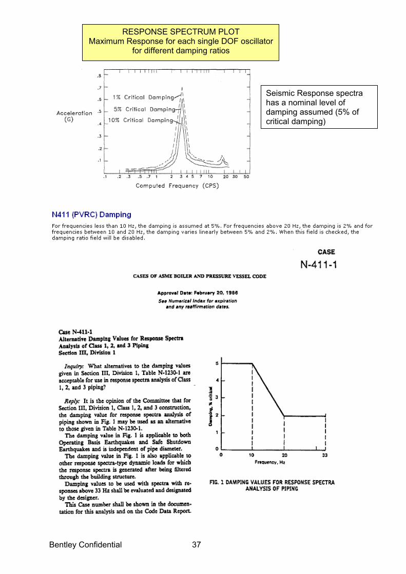
RESPONSE SPECTRUM PLOT Maximum Response for each single DOF oscillator
for different damping ratios
Seismic Response spectra has a nominal level of damping assumed (5% of critical damping)
Bentley Confidential 38
Nuclear Regulatory guide 1.60 (published in Dec 1973) describes the requirements for generating a design seismic response spectra for nuclear power plants. Since response spectrum is based on SDOF system, the response can be approximately represented by a sine function. Displacement= A sin(wt+phase) Velocity = Aw.cos(wt+phase) Acceleration = -Aw2.sin(wt+phase) The maximum displacement A, maximum velocity Aw and maximum acceleration Aw2 are related using the SDOF angular frequency w=2* π *Frequency Due to this fact, the displacement, acceleration and velocity spectra can be plotted on a single log-log plot also called tripartite plot. The plot provided in AutoPIPE notes corresponds to NRC displacement spectra included in the AutoPIPE directory. All these spectra are normalized to a maximum ground acceleration of 1g. Damping of structure can reduce the response. Effects of damping can be seen on the NRC tripartite plot. Notice that for a 0.5% damped system an amplification factor of 6.0 is expected (6g). This can be more for lower damping. A maximum DLF of 2.0 is not appropriate for long duration loads such as earthquake. It is only applicable for short transient loads, like relief valve or water hammer loads. Damping is small when piping does not move at support points generating friction. For example for vertical vibrations on a long span pipeline, a damping ratio of 0.2 may be used. When pipe is expected to move at support points, damping ratios of 2%-5% are reasonable. For submerged piping a damping of 10% or more commonly used. Although the response appears to be a smooth line, this is not actually the case. As you discretize the SDOF frequency (more points on x-axis), the curve will have an erratic shape with several peaks and ‘valleys’. Unfortunately using such spectrum at a valley location will be un-conservative. This is due to the fact that the structural frequency will change during an earthquake. This change is caused by material yield or support failure. A design response spectrum like NRC ones provided in AutoPIPE are the result of averaging multiple earthquake spectra and enveloping the resulting spectrum. NRC has a procedure to generate a design spectrum from a single earthquake record. The procedure involves ignoring the valley points.

Bentley Confidential 39
Response spectrum is more suited for design than time history analysis for the reason mentioned above. The only disadvantage of response spectrum is that it is limited to a linear system. For very important structure, nonlinear time history analysis is sometimes performed. For such cases, 15 or 20 such time history cases are performed and the time histories themselves are generated from a design response spectrum. These are called response spectrum compatible earthquakes. Each response spectrum can correspond to infinite number of time histories as the phase information is lost in a response spectrum. The UBC and more recently the IBC has a procedure to generate a design response spectrum based earthquake geographic zone, soil conditions and other factors. The procedure does not involve any actual earthquake time records. Piping is typically supported on building structures. Regular ground response spectra may not be appropriate for such piping. A special spectrum called floor response spectrum is typically used. The higher the floor the more response is expected. AutoPIPE provides a way to scale parts of your piping for such effects using point and member EQ scale factors.

Bentley Confidential 40
Spectral Data follows the rules: Ai = -ωi^2 * displacement = ωi*velocity
where: Acceleration = Ai ωi = 2*π*(frequency)
Example: 5 Hz (2. π .5 = 31.416 rad/s) , read response displacement = 2”, Read velocity = 60 in/s (2 * 31.416 = 62.83 in/s), read acceleration = 5g = 5*386.16 = 1930.61 in^2 (2 * 31.416^2 = 1973.9 in^2/s)
60
Zero period accelertion, ZPA
Low Frequency flexible range, relative displacement = ground displacement
33Hz
NRC Guide 1.60 RESPONSE SPECTRUM PLOT Maximum accelerations, velocities and displacements
A and above – Rigid high frequency (acceleration loads = static i.e. ZPA & mode independent, no relative displacement between mass & their supports) D and below – Flexible low frequency cutoff (System forces due to mass acceleration = 0)

Bentley Confidential 41
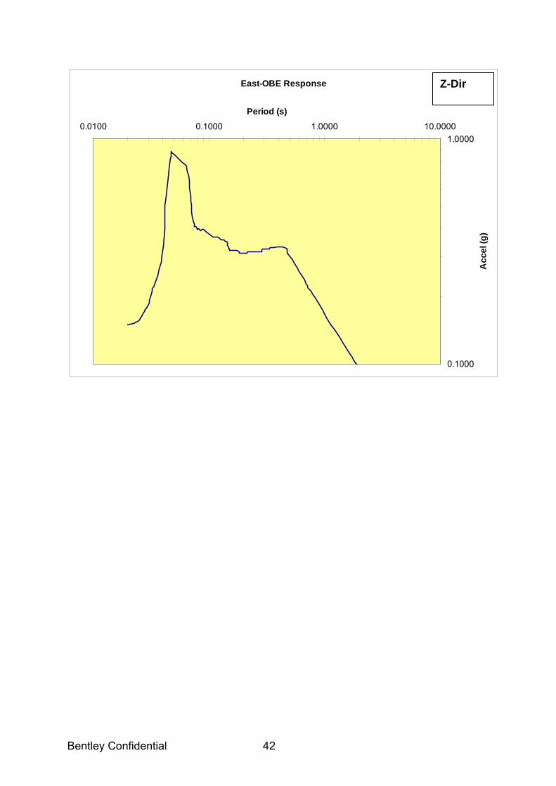
North-OBE Response
0.1000
1.00000.0100 0.1000 1.0000 10.0000
Period (s)
Acc
el (g
)
South-OBE Response
0.1000
1.00000.0100 0.1000 1.0000 10.0000
Period (s)
Acc
el (g
)
X-Dir
Y-Dir
Typical Response Spectrum Plots
Bentley Confidential 42
East-OBE Response
0.1000
1.00000.0100 0.1000 1.0000 10.0000
Period (s)
Acc
el (g
)
Z-Dir
Bentley Confidential 43
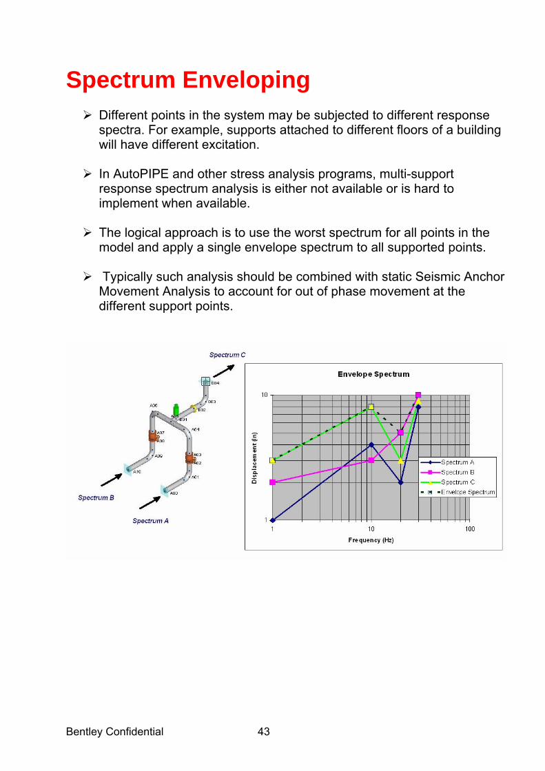
Spectrum Enveloping
Different points in the system may be subjected to different response spectra. For example, supports attached to different floors of a building will have different excitation.
In AutoPIPE and other stress analysis programs, multi-support response spectrum analysis is either not available or is hard to implement when available.
The logical approach is to use the worst spectrum for all points in the model and apply a single envelope spectrum to all supported points.
Typically such analysis should be combined with static Seismic Anchor Movement Analysis to account for out of phase movement at the different support points.
Bentley Confidential 44
Static Correction
To capture total dynamic response of a structure all possible modes should be captured.
For a large system this is impractical due to large number of modes.
High frequency modes that do not contribute significantly to the final response can be approximated using static correction methods.
Static correction is approximate and may not predict local response
Zero Period Acceleration (ZPA)
The structure is subjected to the peak ground acceleration. Entire mass of the structure is considered.
Static response is obtained for the structure.
Larger of the static and dynamic response is used.
Available all Dynamic Analyses
Missing Mass Correction
The amount of mass captured by all extracted modes is subtracted from the total mass.
The structure is subjected to acceleration equal to the cut-off frequency. Only the uncaptured mass is considered.
Static response is obtained for the structure.
The static response is combined with the dynamic response using the specified combination method.
Available for harmonic, response & force spectrum only.
Bentley Confidential 45
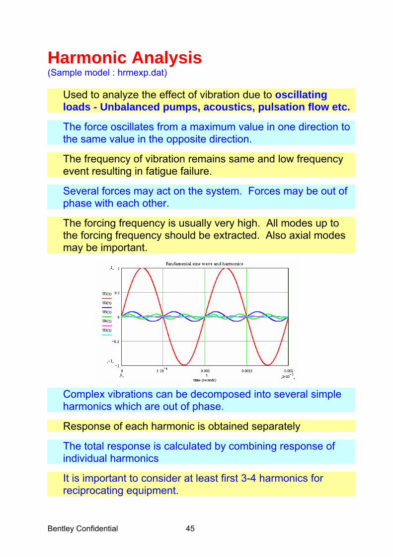
Harmonic Analysis (Sample model : hrmexp.dat)
Used to analyze the effect of vibration due to oscillating loads - Unbalanced pumps, acoustics, pulsation flow etc.
The force oscillates from a maximum value in one direction to the same value in the opposite direction.
The frequency of vibration remains same and low frequency event resulting in fatigue failure.
Several forces may act on the system. Forces may be out of phase with each other.
The forcing frequency is usually very high. All modes up to the forcing frequency should be extracted. Also axial modes may be important.
Complex vibrations can be decomposed into several simple harmonics which are out of phase.
Response of each harmonic is obtained separately
The total response is calculated by combining response of individual harmonics
It is important to consider at least first 3-4 harmonics for reciprocating equipment.
Bentley Confidential 46
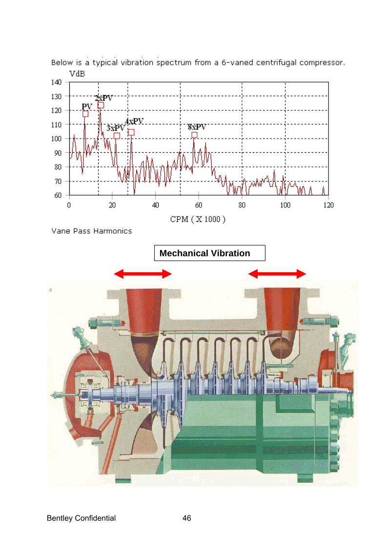
Mechanical Vibration

Bentley Confidential 47
Force Spectrum Analysis
Used to analyze response of a system due to short duration, impulsive loads
• Water hammer • Relief valve blow down, etc.
The force is usually given in terms of a force time history. Magnitude of force is plotted against time. To obtain most accurate results, a Direct Integration Time History analysis is required. However, this procedure is very complex and time consuming. Can take hours on a personal computer. Force spectrum is an alternate. A time history can be converted into force spectrum using Duhemal's integration method. The force spectrum is applied at location where force is acting. Assumes all forces are acting at the same time. Higher modes are important to determine the response of systems due to such loads. For water-hammer type analysis, axial modes (usually high frequency) are important.
Bentley Confidential 48
Seismic Anchor Movement Analysis
Predicts stresses on piping system due to differential movement of buildings or floors during a seismic event. Required by nuclear Class II and III piping codes All supported points moving together as a group are said to be in phase. e.g. all points on a floor are in phase Response is determined using static linear analysis Response spectrum is typically combined with SAM e.g. Abs Sum to assess worse case response. PROCEDURE
1. Piping system is solved for SAM in global X direction for Phase 1
2. Piping system is solved for SAM in global X direction for each remaining phase
3. Maximum response in X direction is calculated using absolute sum.
4. Step 1, 2 and 3 are repeated for global Y and Z directions
Final response is calculated by combining responses of global X, Y and Z directions using the SRSS combination method.
Bentley Confidential 49
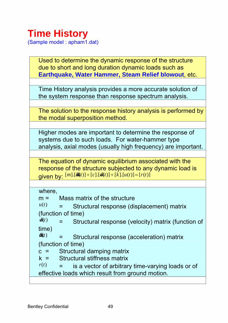
Time History (Sample model : apham1.dat)
Used to determine the dynamic response of the structure due to short and long duration dynamic loads such as Earthquake, Water Hammer, Steam Relief blowout, etc. Time History analysis provides a more accurate solution of the system response than response spectrum analysis. The solution to the response history analysis is performed by the modal superposition method. Higher modes are important to determine the response of systems due to such loads. For water-hammer type analysis, axial modes (usually high frequency) are important. The equation of dynamic equilibrium associated with the response of the structure subjected to any dynamic load is given by: )]([)](].[[)](].[[)](].[[ trtuktuctum =++ &&& where, m = Mass matrix of the structure
)(tu = Structural response (displacement) matrix (function of time) )(tu& = Structural response (velocity) matrix (function of time)
)(tu&& = Structural response (acceleration) matrix (function of time) c = Structural damping matrix k = Structural stiffness matrix r t( ) = is a vector of arbitrary time-varying loads or of effective loads which result from ground motion.
Bentley Confidential 50
Assumptions and Limitations:
A single damping ratio is assumed for all modes. The same time step will be used for all modes. Time history files do not support displacement or velocity input only accelerations or force.
All supports are considered linear for this analysis i.e. nonlinear behavior of supports is not considered. This is consistent with assumption made for other dynamic analyses.
Acceleration inputs will be applied to all free degrees of freedom with mass. The user cannot input accelerations for specific points. The user will not be able to prescribe displacement, acceleration, or velocity of supported points. However support displacements can be modeled by entering forces equal to the displacement times support stiffness.
Plotting of time history response at individual points is not available.
Bentley Confidential 51
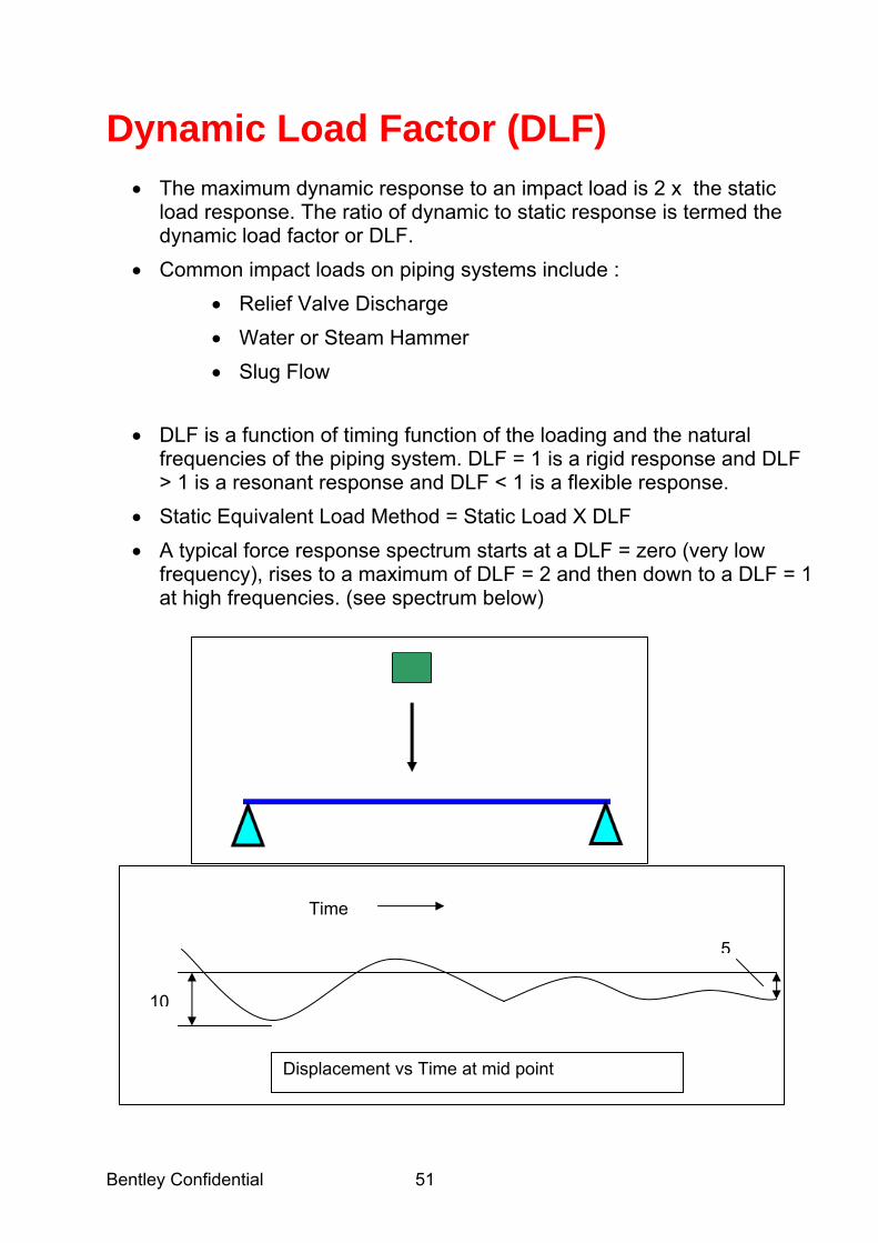
Dynamic Load Factor (DLF)
• The maximum dynamic response to an impact load is 2 x the static load response. The ratio of dynamic to static response is termed the dynamic load factor or DLF.
• Common impact loads on piping systems include : • Relief Valve Discharge • Water or Steam Hammer • Slug Flow
• DLF is a function of timing function of the loading and the natural frequencies of the piping system. DLF = 1 is a rigid response and DLF > 1 is a resonant response and DLF < 1 is a flexible response.
• Static Equivalent Load Method = Static Load X DLF • A typical force response spectrum starts at a DLF = zero (very low
frequency), rises to a maximum of DLF = 2 and then down to a DLF = 1 at high frequencies. (see spectrum below)
10
5
Displacement vs Time at mid point
Time
Bentley Confidential 52
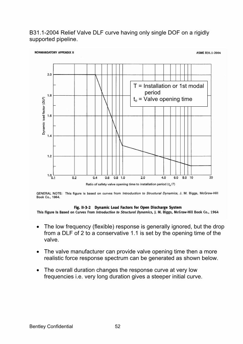
B31.1-2004 Relief Valve DLF curve having only single DOF on a rigidly supported pipeline.
• The low frequency (flexible) response is generally ignored, but the drop from a DLF of 2 to a conservative 1.1 is set by the opening time of the valve.
• The valve manufacturer can provide valve opening time then a more realistic force response spectrum can be generated as shown below.
• The overall duration changes the response curve at very low frequencies i.e. very long duration gives a steeper initial curve.
T = Installation or 1st modal period to = Valve opening time

Bentley Confidential 53
Determine the DLF Factor. Define time history load TEST.TIH starting at time 0 and load = 89000N
Convert Time history load file to force spectrum [Load/Convert to Force Spectrum]
Notice at 20.4 to 510 Hz, the force is about 176000N giving a DLF of about 2.

Bentley Confidential 54
At very high frequency, >2000 Hz, it is 105480 with DLF= 105480 / 89000 = 1.1 The rise time of 0.0004 sec appears unrealistic. If changed to 0.01 sec the force spectrum becomes:
Test Forcing Function
0
10000
20000
30000
40000
50000
60000
70000
80000
90000
1000000 0.01 0.02 0.03 0.04 0.05
Time (s)
Forc
e (N
)
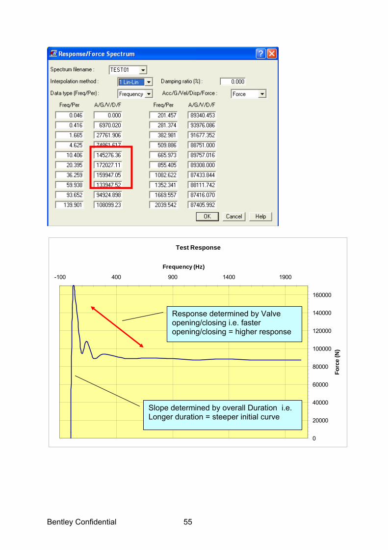
Bentley Confidential 55
Test Response
0
20000
40000
60000
80000
100000
120000
140000
160000
-100 400 900 1400 1900
Frequency (Hz)
Forc
e (N
)
Slope determined by overall Duration i.e. Longer duration = steeper initial curve
Response determined by Valve opening/closing i.e. faster opening/closing = higher response

Bentley Confidential 56
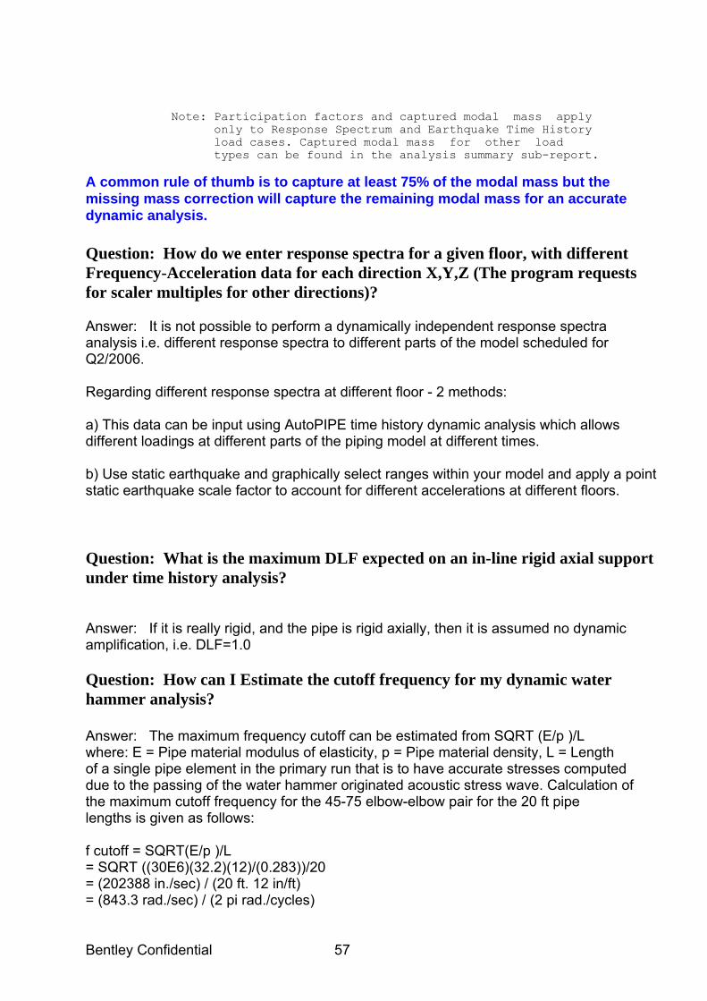
Question: What are the Participation Factors and the Captured Modal Mass in the frequency report?
Answer: The participation factor is a measure of the importance of the mode in earthquake type load. The captured modal mass is another way of quantifying the importance of the mode and the two are related. The captured modal mass percentage shows how much of the response is attributed to a particular mode and also shows the mode orientation (X, Y or Z). The sum of modal masses should be 100% if all modes are counted. But since many modes are not counted, the sum is less than 100 and hence the importance of the ZPA and missing mass options for dynamic analysis. Please refer to the topic "Missing Mass and ZPA Correction" in the online help for more information. The participation factors are calculated from the product of the mode shape, the mass matrix and a vector of ones. For mode i the participation factor is calculated as: Participation_Factor_i= Transpose(ModeShape_i) * MassMatrix * {1} The mode shape is mass normalized. The above equation is used three times for X, Y and Z directions. The mass participation report illustrates how sensitive each of the piping system’s modes are to the dynamic loading. High modal participation factors indicate that the mode is easily excited by the applied dynamic forces. If subsequent displacement reports indicate high dynamic responses then the modes having high participation factors must be dampened or eliminated. Once a particular mode is targeted as being a problem, it may be viewed in the mode shape report, or graphically via the animated mode shape plots.
-------------------------------------------------------------------------------- APHAM1A_SI_1 09/08/2005 SAMPLE MODEL OF WATER HAMMER BENTLEY 10:58 AM AutoPIPE+8.60 RESULT PAGE 3 -------------------------------------------------------------------------------- F R E Q U E N C I E S Mode Freq. Period Participation Factors Captured Modal Mass (Percent) Number (Hertz) (Sec) X Y Z X Y Z Average ------ ------- ------- ------- ------- ------- ------- ------- ------- ------- 1 2.7710 0.361 3.01 0.00 -2.75 14.284 0.000 11.868 8.717 2 2.9835 0.335 -0.13 0.00 3.90 0.027 0.000 23.934 7.987 3 3.1907 0.313 4.33 0.00 1.90 29.479 0.000 5.703 11.727 4 8.8320 0.113 -0.27 0.00 -0.10 0.111 0.000 0.017 0.042 21 30.9498 0.032 -0.14 0.01 1.95 0.030 0.000 5.981 2.004 22 32.1595 0.031 -0.07 -0.40 -0.03 0.007 0.248 0.001 0.085 Total captured modal mass (%) 66.680 27.597 54.593 49.623 Total system weight = 11147.2 Kg
Bentley Confidential 57
Note: Participation factors and captured modal mass apply only to Response Spectrum and Earthquake Time History load cases. Captured modal mass for other load types can be found in the analysis summary sub-report.
A common rule of thumb is to capture at least 75% of the modal mass but the missing mass correction will capture the remaining modal mass for an accurate dynamic analysis. Question: How do we enter response spectra for a given floor, with different Frequency-Acceleration data for each direction X,Y,Z (The program requests for scaler multiples for other directions)? Answer: It is not possible to perform a dynamically independent response spectra analysis i.e. different response spectra to different parts of the model scheduled for Q2/2006. Regarding different response spectra at different floor - 2 methods: a) This data can be input using AutoPIPE time history dynamic analysis which allows different loadings at different parts of the piping model at different times. b) Use static earthquake and graphically select ranges within your model and apply a point static earthquake scale factor to account for different accelerations at different floors. Question: What is the maximum DLF expected on an in-line rigid axial support under time history analysis? Answer: If it is really rigid, and the pipe is rigid axially, then it is assumed no dynamic amplification, i.e. DLF=1.0 Question: How can I Estimate the cutoff frequency for my dynamic water hammer analysis? Answer: The maximum frequency cutoff can be estimated from SQRT (E/p )/L where: E = Pipe material modulus of elasticity, p = Pipe material density, L = Length of a single pipe element in the primary run that is to have accurate stresses computed due to the passing of the water hammer originated acoustic stress wave. Calculation of the maximum cutoff frequency for the 45-75 elbow-elbow pair for the 20 ft pipe lengths is given as follows: f cutoff = SQRT(E/p )/L = SQRT ((30E6)(32.2)(12)/(0.283))/20 = (202388 in./sec) / (20 ft. 12 in/ft) = (843.3 rad./sec) / (2 pi rad./cycles)

Bentley Confidential 58
= 134.2 Hz. Question: Do you have any span guideline to avoid piping vibration? Answer: The following span guidelines to avoid resonance from compressor accoustic vibration. Typically for low speed motors e.g. 300rpm use multiplier 2.4 up to 4.0, i.e. 5hz x 2.4 = 12hz. High speed compressors e.g. 1800rpm use multiplier 1.4, i.e. 30hz x 1.4 = 42hz. Then calculate pipe span based on this fundamental frequency (1st mode) for both fixed and simply supported ends. A typical pipe behaves somewhere between these two boundary conditions. Ref Roark Table 36 case 1b, 2b fn = Kn/2/pi *SQRT (Eig/w/L^4) hence Span (L) = E.I.Kn2/W/f12
where : W = weight /unit length (kg/mm) I = moment of inertia (mm4) f1 = frequency (Hz) E = Youngs Modulus (Mpa) kn = 3.55 (Fixed Ends), 1.57 (simply supported) Question: My Stress due to dynamic response spectrum analysis exceeds the code allowable? Answer: The response can usually be changed by increasing or decreasing the frequency of the mode shape causing the dynamic response. Using the animation of the dynamic response spectrum analysis, and find the mode shape which closely matches this response. The solution is usually adding a restraint at a point of large modal displacement which typically increases the modal frequency. Since the dynamic load factor (DLF) drops with increasing frequency, the best solution is to increase the 1st modal frequency. This is done by increasing the stiffness of the system e.g. adding supports or increasing support stiffness or reducing its mass e.g. thinner pipe or move valves closer to support locations.
Also refer to AutoPIPE FAQ’s and technotes http://selectservices.bentley.com/en-US/Support/Support+Tools/TechNotes+and+FAQs/Bentley+AutoPIPE/Index.htm in particular technote 8274 - Compressor Vibration Method

Bentley Confidential 59
Fluid Transient (Sample model : apham1.dat)
Used to determine the force-time histories along a single pipeline due to fluid transient events such as valve closures, pump shutdowns, flow demand changes, pump startups, air venting from lines, failure of flow or pressure regulators, or pipe rupture.
For a piping system with branches, the user must select a single main pipeline in
which to generate the force-time history. The effect of branches on the surge pressure will be ignored.
The shock wave travels back upstream from the valve but the forces are acting downstream. Consider free body diagram below - the +ve pressure rise at the Valve results in higher pressure acting at valve end compared to 1st bend end hence the net force is acting towards the valve (in the direction of the flow). Thus the shock wave (and pressure rise) propagates back up the pipe resulting in leg forces acting in the same direction as the flow.
Bentley Confidential 60
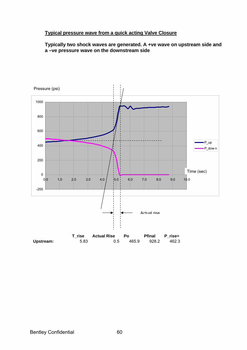
Typical pressure wave from a quick acting Valve Closure Typically two shock waves are generated. A +ve wave on upstream side and a –ve pressure wave on the downstream side
-200
0
200
400
600
800
1000
0.0 1.0 2.0 3.0 4.0 5.0 6.0 7.0 8.0 9.0 10.0
P_up
P_dow n
Time (sec)
T_rise Actual Rise Po Pfinal P_rise= Upstream: 5.83 0.5 465.9 928.2 462.3
Pressure (psi)
Actual rise
Bentley Confidential 61
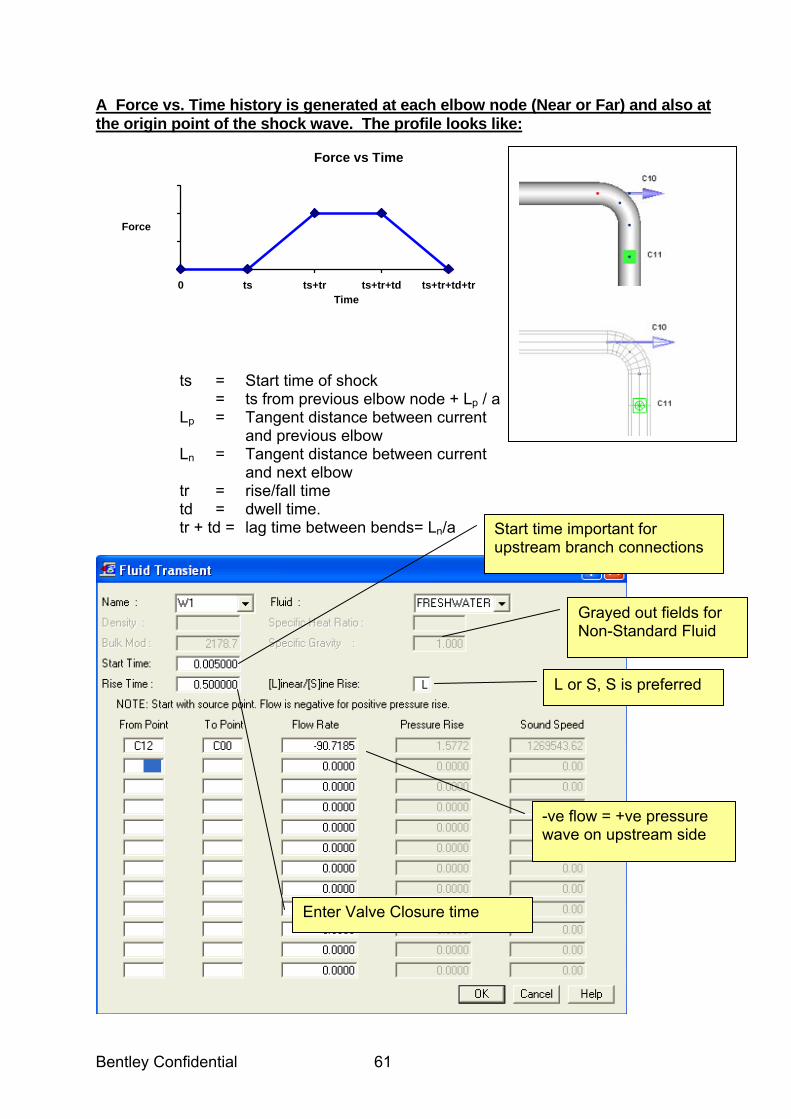
A Force vs. Time history is generated at each elbow node (Near or Far) and also at the origin point of the shock wave. The profile looks like:
where,
ts = Start time of shock = ts from previous elbow node + Lp / a Lp = Tangent distance between current and previous elbow Ln = Tangent distance between current and next elbow tr = rise/fall time td = dwell time. tr + td = lag time between bends= Ln/a
Force vs Time
0 ts ts+tr ts+tr+td ts+tr+td+trTime
Force
Enter Valve Closure time
L or S, S is preferred
Start time important for upstream branch connections
-ve flow = +ve pressure wave on upstream side
Grayed out fields for Non-Standard Fluid
Bentley Confidential 62
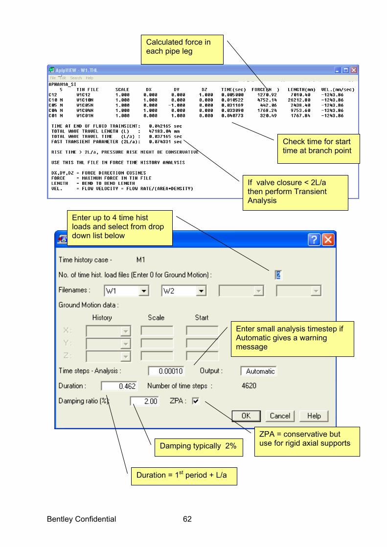
Calculated force in each pipe leg
Check time for start time at branch point
If valve closure < 2L/a then perform Transient Analysis
ZPA = conservative but use for rigid axial supports
Duration = 1st period + L/a
Enter small analysis timestep if Automatic gives a warning message
Enter up to 4 time hist loads and select from drop down list below
Damping typically 2%
Bentley Confidential 63
• The reduction in the magnitude of the hammer loads is best achieved by a slow
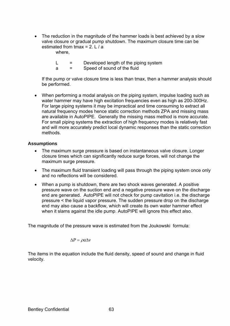
valve closure or gradual pump shutdown. The maximum closure time can be estimated from tmax = 2. L / a
where, L = Developed length of the piping system a = Speed of sound of the fluid If the pump or valve closure time is less than tmax, then a hammer analysis should
be performed.
• When performing a modal analysis on the piping system, impulse loading such as water hammer may have high excitation frequencies even as high as 200-300Hz. For large piping systems it may be impractical and time consuming to extract all natural frequency modes hence static correction methods ZPA and missing mass are available in AutoPIPE. Generally the missing mass method is more accurate. For small piping systems the extraction of high frequency modes is relatively fast and will more accurately predict local dynamic responses than the static correction methods.
Assumptions
• The maximum surge pressure is based on instantaneous valve closure. Longer closure times which can significantly reduce surge forces, will not change the maximum surge pressure.
• The maximum fluid transient loading will pass through the piping system once only and no reflections will be considered.
• When a pump is shutdown, there are two shock waves generated. A positive pressure wave on the suction end and a negative pressure wave on the discharge end are generated. AutoPIPE will not check for pump cavitation i.e. the discharge pressure < the liquid vapor pressure. The sudden pressure drop on the discharge end may also cause a backflow, which will create its own water hammer effect when it slams against the idle pump. AutoPIPE will ignore this effect also.
The magnitude of the pressure wave is estimated from the Joukowski formula:
vaP ∆=∆ ρ The items in the equation include the fluid density, speed of sound and change in fluid velocity.
Bentley Confidential 64
Question: I am performing a steam hammer analysis but when should I use ZPA correction method under Time History analysis? Answer: We recommend to perform two analyses, one with ZPA and one without. For flexible legs (legs with flexible or no axial supports) use no ZPA correction. If the system has pipe legs with rigid axial supports, use ZPA correction to determine realistic loads on these axial supports. Note: ZPA can be very conservative for flexible legs.
Question: How I can be sure I have correctly modeled my fluid transient? Answer: Some key points to check modeling a fluid transient : Define the flow rate with correct sign. Flow rate is positive for negative pressure rise. Note: When a pump is shutdown, there are two shock waves generated. A positive pressure wave on the suction end and a negative pressure wave on the discharge end are generated. The maximum possible negative pressure wave is equal in magnitude to the pump discharge pressure(Ps) less the liquid vapor pressure (Pv). The pressure wave amplitude is calculated in AutoPIPE using the Joukowski formula. Be sure to check your vapor pressure is not below Static - maximum pressure drop (i.e. Ps-Pv) otherwise cavitation will occur
dP = Fluid density*Fluid velocity*speed_of_sound [ vaP ∆=∆ ρ ]
• This pressure wave = dP should be less than Ps-Pv to avoid cavitation. This condition should be avoided since the AutoPIPE results will be invalid. Similarly the pressure rise will be positive upstream of a closed valve and negative downstream of an open valve.
• Typically use default SINE rise function
• Define time history duration as 1st period (1/first modal frequency, hz) + transient duration (as shown in the THL file i.e. TOTAL WAVE TRAVEL TIME (L/a))
• When click ok to the fluid transient check the red highlighted sections of piping are correct.
• Run the modal analysis with cut-off frequency at least 100 to 150hz. Recommended to perform modal followed by time history analysis at both cut-off frequencies to confirm the solution has converge i.e. time history results are similar.
• Run time history with and without ZPA correction. See FAQ Q31. Note: Recommend to set under tools/model options/Edit "Mass points per span" = A to allow the program to automatically perform mass discretization on your model for improved accuracy for the dynamic analysis.

Bentley Confidential 65
Support solution Flexible is better. The restraint should only be stiff enough to sufficiently attenuate the low frequency gross deformation. Question : The AutoPIPE help states “When the rise time several times larger than the 2L/a time, the calculated pressure rise in AutoPIPE might be conservative. For this special case, the use of a fluid simulation software is recommended if P2 case is critical.” What does this mean? Answer: Check for maximum surge pressure (static (362)+ rise (228) =590 psi). This should be added as a second pressure case (P2). Use Tools/Model Options/General and set number of operating cases to 2. Use Select/All Points and follow by Modify/Pressure & Temperature and set design pressure for P2 to 590 psi. When the rise time several times larger than the 2L/a time, the calculated pressure rise in AutoPIPE might be conservative. For this special case, the use of a fluid simulation software is recommended if P2 case is critical and causes an overstress condition in the pipework If P2=590 psi governs the design, that is critical, the use of fluid simulation software is recommended since AutoPIPE value would be too conservative.
Bentley Confidential 66
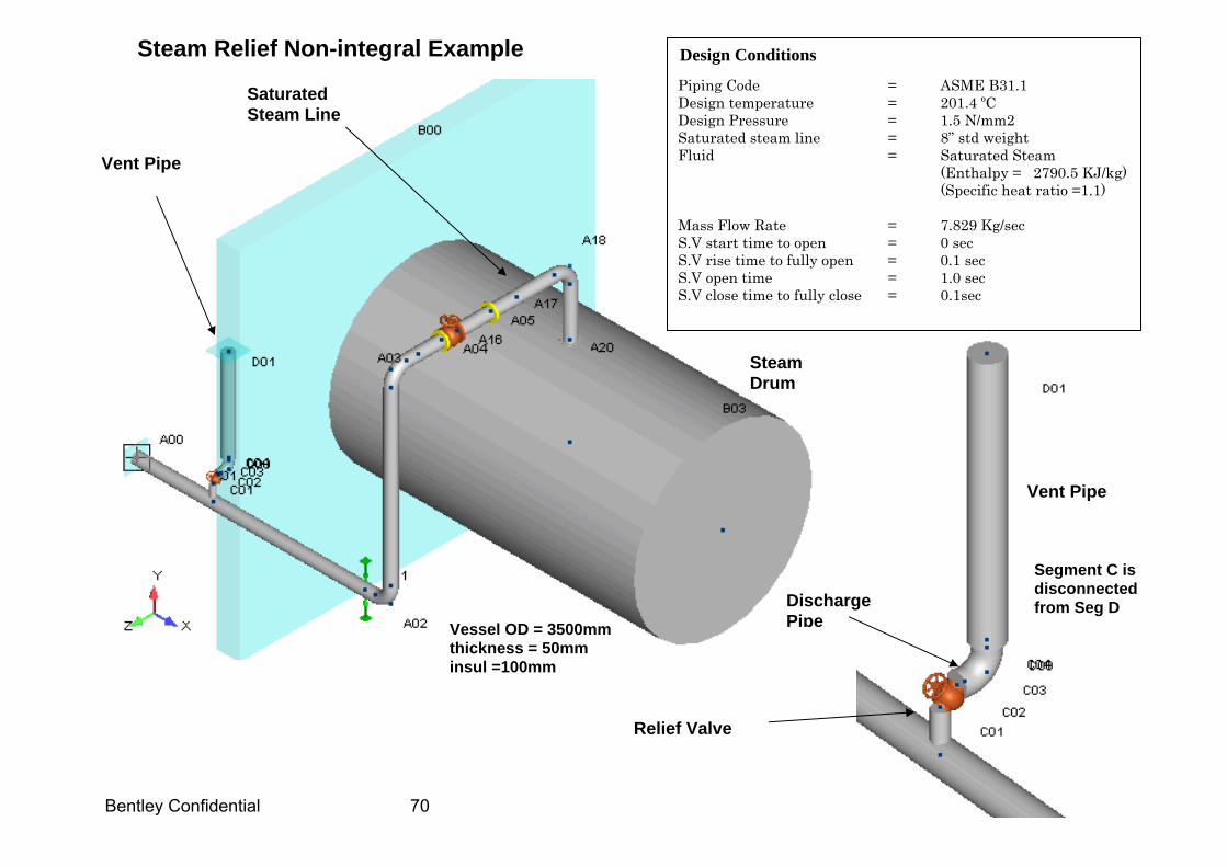
Steam Relief (Sample model : ap50SR1.dat)
• Used to calculate the thrust loads at the valve exit piping due to discharge of the relief valve and automatically generate the time history files to perform a dynamic time history analysis.
• Only the thrust loads at the valve exit piping will be calculated in accordance with
Appendix II of ASME B31.1 code. Since these thrust loads are dynamic in nature, they can be analyzed more accurately using the AutoPIPE time-history solution than using ASME 31.1 Appendix II section 3.5.1.
• The steam relief event is dependent on the type of vent piping either discharging to
atmosphere or a closed manifold. Using AutoPIPE, the configuration of relief and vent piping is modeled as either:
• Open discharge to atmosphere- with non-integral relief and vent piping • Open discharge to atmosphere- with integral relief and vent piping • Closed discharge to manifold - with integral relief and vent piping
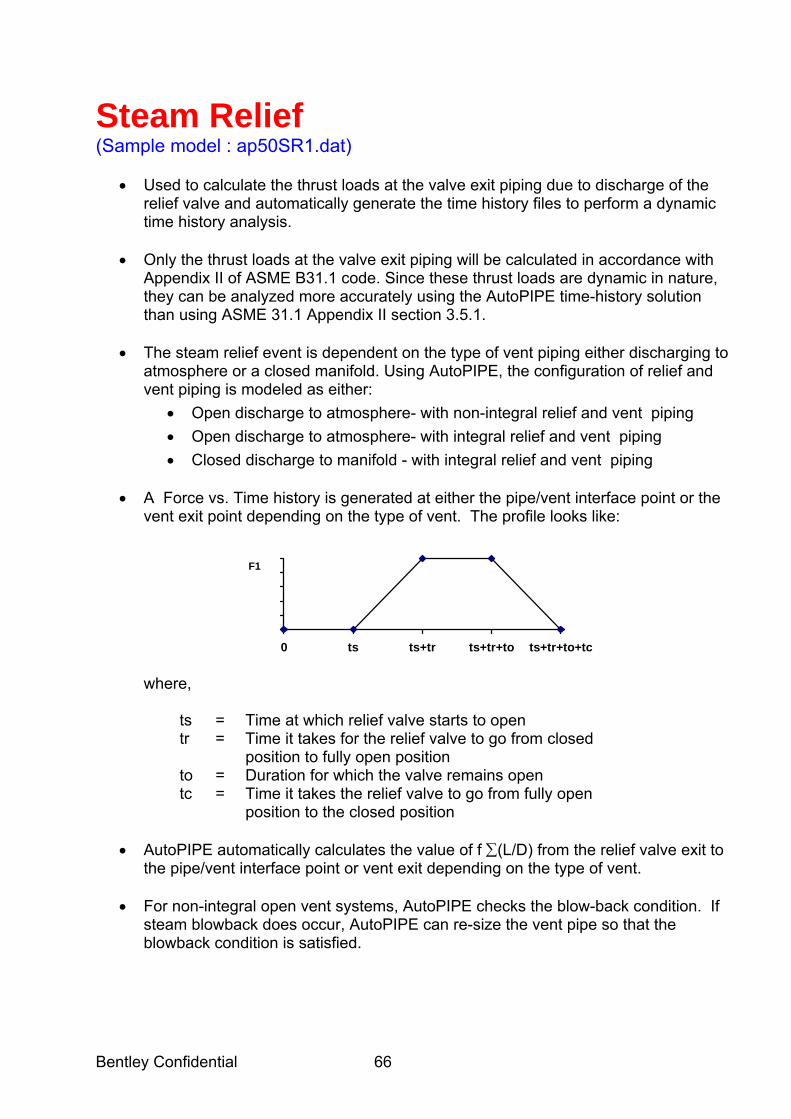
• A Force vs. Time history is generated at either the pipe/vent interface point or the
vent exit point depending on the type of vent. The profile looks like:
0 ts ts+tr ts+tr+to ts+tr+to+tc
F1
where, ts = Time at which relief valve starts to open tr = Time it takes for the relief valve to go from closed position to fully open position to = Duration for which the valve remains open tc = Time it takes the relief valve to go from fully open position to the closed position
• AutoPIPE automatically calculates the value of f ∑(L/D) from the relief valve exit to the pipe/vent interface point or vent exit depending on the type of vent.
• For non-integral open vent systems, AutoPIPE checks the blow-back condition. If
steam blowback does occur, AutoPIPE can re-size the vent pipe so that the blowback condition is satisfied.

Bentley Confidential 67
Enter Valve exit point name, each name = separate report
Quality 1= wet steam , 2 = saturated , 3 = supeheated
Enter manifold pressure for closed discharge, >= atmos
Point 3
Check to create a report for each defined Valve exit point
Point 2
Point 1
Valve opening time
Time Valve remains open
Valve closing time
Bentley Confidential 68
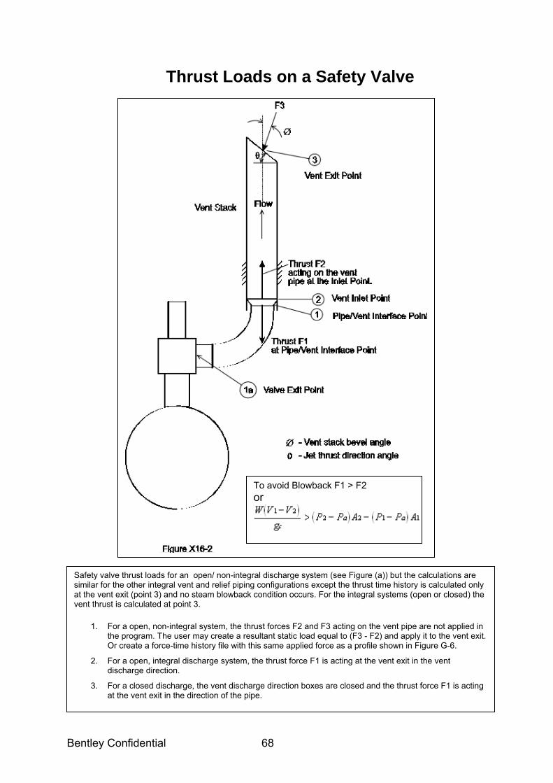
Thrust Loads on a Safety Valve
Safety valve thrust loads for an open/ non-integral discharge system (see Figure (a)) but the calculations are similar for the other integral vent and relief piping configurations except the thrust time history is calculated only at the vent exit (point 3) and no steam blowback condition occurs. For the integral systems (open or closed) the vent thrust is calculated at point 3.
1. For a open, non-integral system, the thrust forces F2 and F3 acting on the vent pipe are not applied in the program. The user may create a resultant static load equal to (F3 - F2) and apply it to the vent exit. Or create a force-time history file with this same applied force as a profile shown in Figure G-6.
2. For a open, integral discharge system, the thrust force F1 is acting at the vent exit in the vent discharge direction.
3. For a closed discharge, the vent discharge direction boxes are closed and the thrust force F1 is acting at the vent exit in the direction of the pipe.
To avoid Blowback F1 > F2 or
Bentley Confidential 69
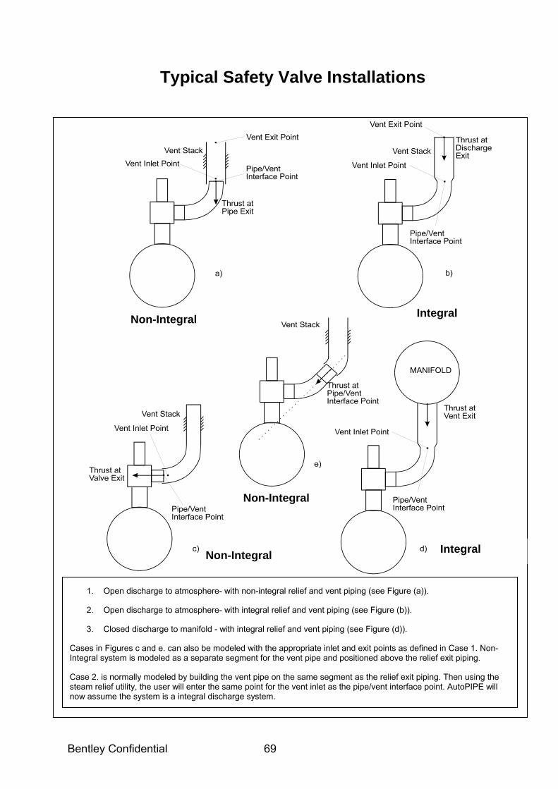
Typical Safety Valve Installations
1. Open discharge to atmosphere- with non-integral relief and vent piping (see Figure (a)).
2. Open discharge to atmosphere- with integral relief and vent piping (see Figure (b)).
3. Closed discharge to manifold - with integral relief and vent piping (see Figure (d)).
Cases in Figures c and e. can also be modeled with the appropriate inlet and exit points as defined in Case 1. Non-Integral system is modeled as a separate segment for the vent pipe and positioned above the relief exit piping.
Case 2. is normally modeled by building the vent pipe on the same segment as the relief exit piping. Then using the steam relief utility, the user will enter the same point for the vent inlet as the pipe/vent interface point. AutoPIPE will now assume the system is a integral discharge system.
Non-Integral Integral
Integral
Non-Integral
Non-Integral
Bentley Confidential 70
Steam Drum
Saturated Steam Line
Vent Pipe
Design Conditions
Piping Code = ASME B31.1 Design temperature = 201.4 ºC Design Pressure = 1.5 N/mm2 Saturated steam line = 8” std weight Fluid = Saturated Steam
(Enthalpy = 2790.5 KJ/kg) (Specific heat ratio =1.1) Mass Flow Rate = 7.829 Kg/sec S.V start time to open = 0 sec S.V rise time to fully open = 0.1 sec S.V open time = 1.0 sec S.V close time to fully close = 0.1sec
Vent Pipe
Relief Valve
Discharge Pipe
Steam Relief Non-integral Example
Segment C is disconnected from Seg D
Vessel OD = 3500mm thickness = 50mm insul =100mm
Bentley Confidential 71
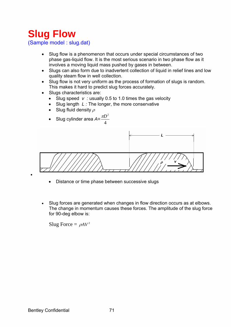
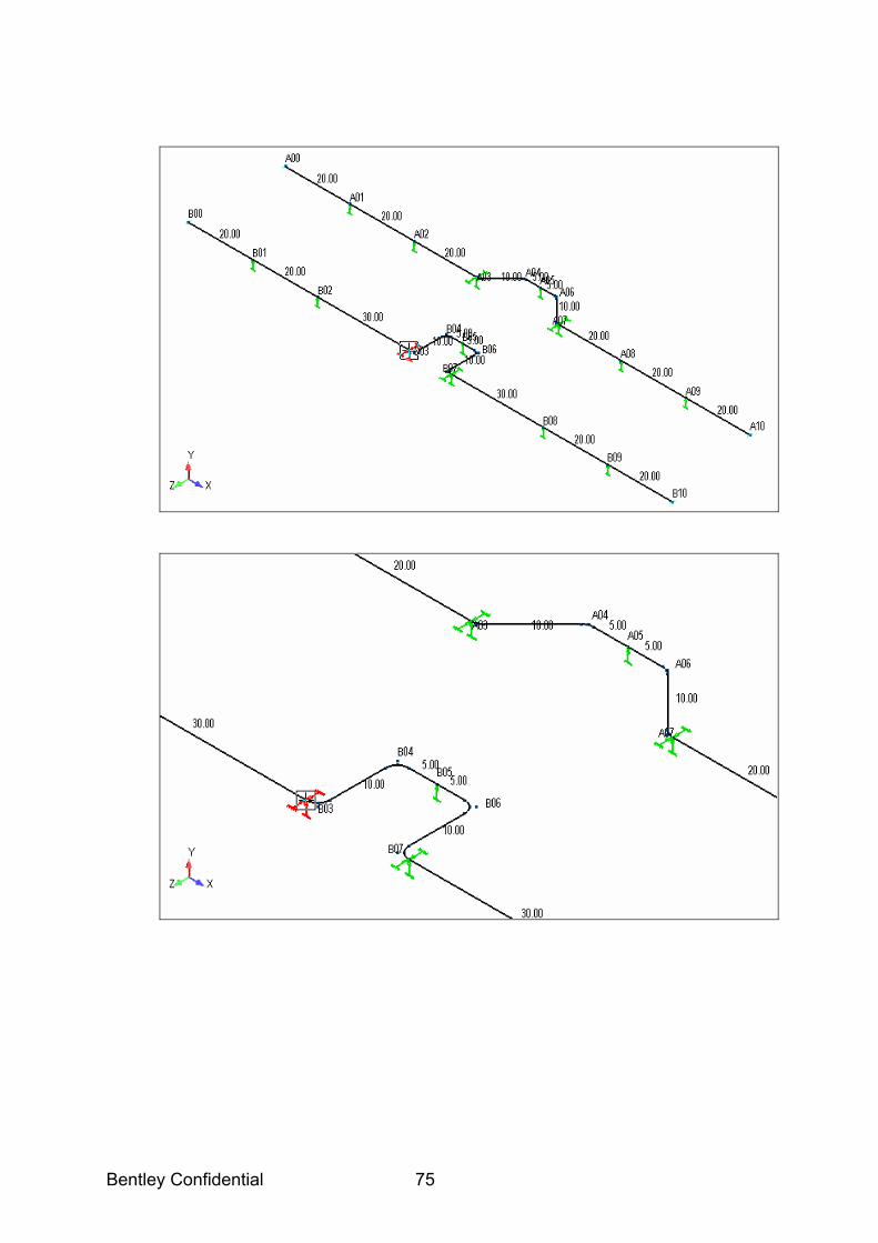
Slug Flow (Sample model : slug.dat)
• Slug flow is a phenomenon that occurs under special circumstances of two phase gas-liquid flow. It is the most serious scenario in two phase flow as it involves a moving liquid mass pushed by gases in between.
• Slugs can also form due to inadvertent collection of liquid in relief lines and low quality steam flow in well collection.
• Slug flow is not very uniform as the process of formation of slugs is random. This makes it hard to predict slug forces accurately.
• Slugs characteristics are: • Slug speed v : usually 0.5 to 1.0 times the gas velocity • Slug length L : The longer, the more conservative • Slug fluid density ρ
• Slug cylinder area A=4
2Dπ
• Distance or time phase between successive slugs
• Slug forces are generated when changes in flow direction occurs as at elbows. The change in momentum causes these forces. The amplitude of the slug force for 90-deg elbow is: Slug Force = 2AVρ
•
Bentley Confidential 72
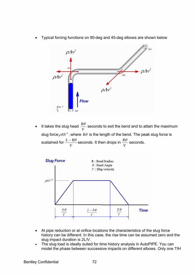
• Typical forcing functions on 90-deg and 45-deg elbows are shown below
• It takes the slug head VRθ
seconds to exit the bend and to attain the maximum
slug force 2AVρ , where θR is the length of the bend. The peak slug force is
sustained for V
RL θ− seconds. It then drops in VRθ
seconds.
• At pipe reduction or at orifice locations the characteristics of the slug force history can be different. In this case, the rise time can be assumed zero and the slug impact duration is 2L/V.
• The slug load is ideally suited for time history analysis in AutoPIPE. You can model the phase between successive impacts on different elbows. Only one TIH

Bentley Confidential 73
file and one THL file need to be entered for each slug. The TIH file profile is shown above. The THL file defines points of application of the TIH file and the direction of load application. It also specifies the time the load will act at each point. A force will be applied at each elbow Near and Far points as shown in the sketch.
• The TIH file depends on slug length, but the THL does not. THL vary with slug speed.
• Most of the response to slug flow is primarily caused by low frequency modes that have large modal displacements in the direction of slug loading.

Bentley Confidential 74
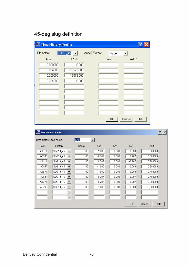
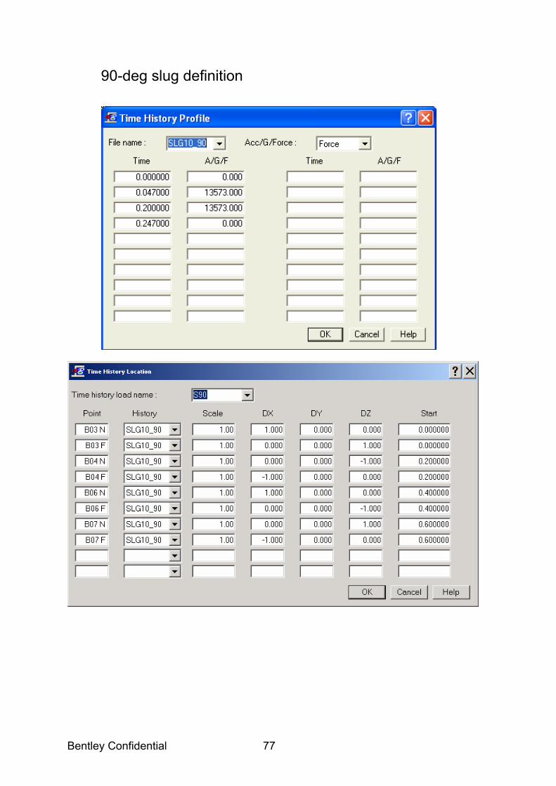
Sample Slug Problem: ASME B31.4 Pressure: 1.034 N/mm2 Temperature: 93.3 deg.C Slug Length = 3.05 m Fluid density = 800.92 kg/m3 Fluid velocity = 15.24 m/sec Fluid diameter = 304.8mm (12 inches i.e.12”STD), Fluid area = 0.072966 m2 Fluid Force: 2AVρ = 800.92*0.072966*15.242 = 13573 N 45-deg bends:
Tr=VRθ
= 1.5*1.57/50/2 = 0.024 seconds
Td = V
RL θ− = 0.176 sec
Tr+Td = 0.2 sec 2Tr+Td = 0.224 sec 90-deg bends:
Tr=VRθ
= 1.5*1.57/50 = 0.047 seconds
Td = V
RL θ− = 0.153 sec
Tr+Td = 0.2 sec 2Tr+Td = 0.247 sec
Bentley Confidential 75
Bentley Confidential 76
45-deg slug definition
Bentley Confidential 77
90-deg slug definition
Bentley Confidential 78
Submerged Piping and Wave Loads (Sample model : RISER_SEABED_SOIL_1.dat and RISER_SEABED_VSTOPS_1.dat)
• Submerged piping is subjected to upward buoyant force reducing its effective weight
• The upward force is proportional to the volume of fluid displaced • Buoyancy force is modeled as distributed load on member. Partially
submerged members are considered loaded with effective force WAVE
• Theories that predict motion of water particles due to wave action 1) Airy 2) Stokes' (up to 5th order) 3) Stream function
• Each theory is valid within its own regime
• These theories determine the velocity and acceleration of water particles due to wave action
• Calculated velocity and acceleration values are used to determine force
on piping system using the Morrison equation 1) Drag force 2) Inertia force 3) Lift force
• The force is applied as distributed load on member DYNAMICS
• Natural frequencies of submerged piping system are lower than frequencies of unsubmerged piping
• The body of water interacts with pipes during motion of pipe.
• This interaction is considered using Added Mass concept
Bentley Confidential 79
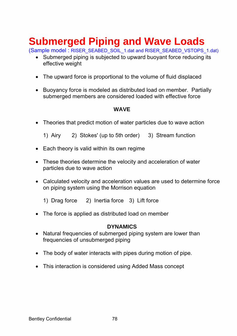
Modeling Riser & Sea bed piping Two modeling approaches shown below:
A) Model : Riser_Seabed_soil_2 This model uses soil properties to simulate the pipeline laying on seabed as a semi-embedded pipe which means soil stiffnesses with all reasonable calculated values for horizontal pipe (including submerged effect on soil) except vertical up resistance K1, P1 and K2 = 0.
See sample soil properties
--------------------------------------------------------------------------------
RISER_SEABED_SOIL_2
06/09/2005 SAMPLE RISER/SEABED BENTLEY
09:43 AM SEABED = SOIL AutoPIPE+8.60 MODEL PAGE 3
--------------------------------------------------------------------------------
SOIL PROPERTIES
Soil Initial K Yield P Final K Yield disp
ID Dirn (Kg/m/mm ) (Kg/m ) (Kg/m/mm ) (mm )
------ ------- ---------- --------- ---------- ----------
A Horiz. 500.000 4000.000 0.100 8.0000
Long 20.000 250.000 0.100 12.5000
Vert Up 0.000 0.000 0.000
Vert Dn 600.000 29999.998 0.100 49.9999
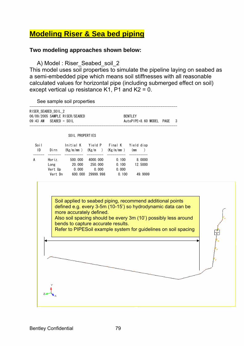
Soil applied to seabed piping, recommend additional points defined e.g. every 3-5m (10-15’) so hydrodynamic data can be more accurately defined. Also soil spacing should be every 3m (10’) possibly less around bends to capture accurate results. Refer to PIPESoil example system for guidelines on soil spacing
Bentley Confidential 80
e.g. typical hydrodynamic data defined for the seabed piping including non-zero lift coefficient.
Typical Hydrodynamic data defined for the riser, zero lift coefficient
Soil shown in blue using view/show /soil
Bentley Confidential 81
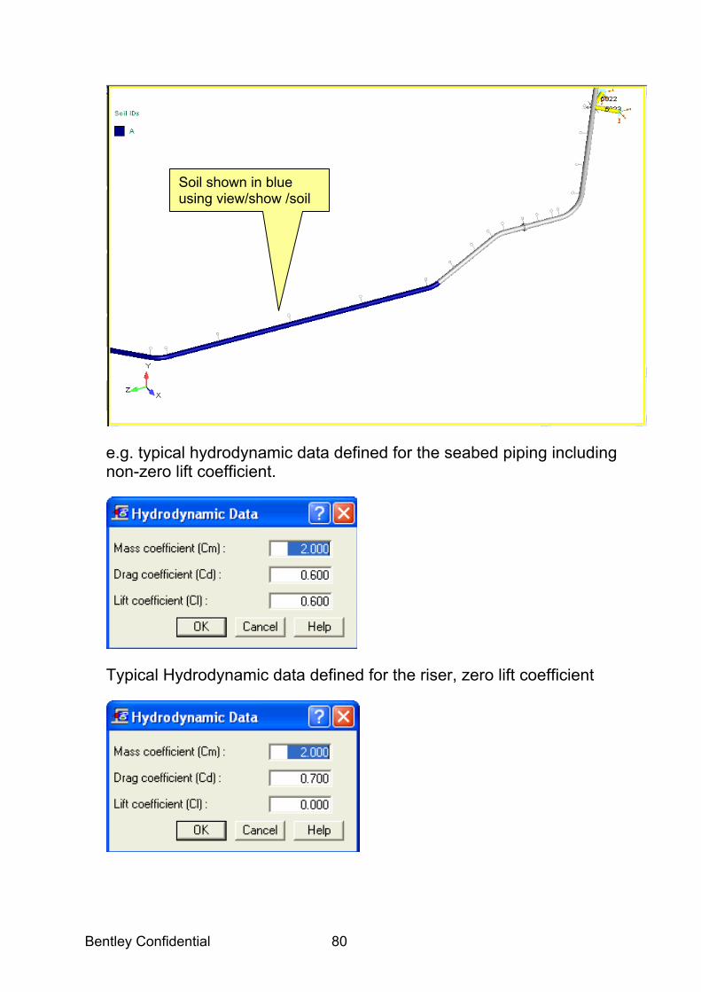
Note: To model stiffness of concrete mattresses restraining the pipe. Two approaches are: A. Insert soil over this area with equivalent stiffness to match rigidity of
mattresses B. Insert V-stops with high friction e.g. much greater than 1.0 Modeling Riser Clamps:
To model weight of concrete mattresses: Either a) Add additional weight using insulation thickness and density b) Uniform distributed load
Attach frame structural members (in this case pipe) to the riser then disconnect by renaming the frame point name (same for both frames). Connect guide from the riser point to the common frame point with gaps and friction e.g. 0.3. Anchor the ends of the frame and apply displacements in each of the wave cases [simulates riser clamp attachment is connected and moves with the platform].
Recommended point spacing along riser is every 8 to 10 feet (2.5 to 3m) to provide adequate mass discretization so the program can capture the distributed wave loading accurately across the riser pipe.
Note: Riser pipes are typically sloped at 10 to 15 deg and guide supports on the riser will be normal to the pipe axis and the reaction loads normal to the pipe can be seen in the a support forces report which shows Local and global displacement's and reactions.
Bentley Confidential 82
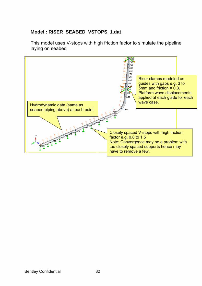
Model : RISER_SEABED_VSTOPS_1.dat This model uses V-stops with high friction factor to simulate the pipeline laying on seabed
Hydrodynamic data (same as seabed piping above) at each point
Closely spaced V-stops with high friction factor e.g. 0.8 to 1.5 Note: Convergence may be a problem with too closely spaced supports hence may have to remove a few.
Riser clamps modeled as guides with gaps e.g. 3 to 5mm and friction = 0.3. Platform wave displacements applied at each guide for each wave case.
Bentley Confidential 83
Key Modeling Points: Defining a Wave model Yes if you define the 2 loadings below this is normally sufficient to provide reasonable static results for riser modeling. a) Wave + current loading b) buoyancy loading Note: AutoPIPE does not automatically include the effect of buoyancy with the wave loading. Buoyancy parameters must be specified using the Analyze/Buoyancy command. The loads due to buoyancy are automatically placed in the gravity load case (GR) by AutoPIPE. Therefore, a combination should be defined which includes GR and the load case which holds the wave loading to see the total effect on a submerged piping system. Some comments on a typical RISER model: a) You do not need to model so many points from bend e.g B16 since the section of piping is buried or has soil properties, autopipe automatically calculates soil springs based on the soil spacing specified. b) Is your water elevation = 0 correct? This means the water surface is at a global y-coord = 0 i.e 28.23ft below anchor A00. c) Current velocity seems high? d) Coeff of drag is typically 1.0 and coeff of inertia = 2.0 e) Your wave direction is required to be defined e.g 1,0,0 is in the global X direction f) You need to input all 5 data pairs for the current loading otherwise the program may get confused with 2 different current velocities at depth = 0. Note: It is important to understand the non-linear load sequencing. The default load sequence which has the wave/current loading following the gravity cold condition but you may wish to change the sequence to consider Gr -> T1 -> U1, U2 i.e. wave cases U1, U2 etc are applied in the hot operating condition. See Q17 & Q18 in attached AutoPIPE FAQ's Question 4: What is an appropriate way to model a offshore riser? Answer: It is important to add many points along the riser section of pipe e.g. at approximately every 8 to 10 feet to provide adequate mass discretization so the program can capture the distributed wave loading accurately across the riser pipe. Riser pipes are typically sloped at 10 to 15 deg and guide supports on the riser will be normal to the pipe axis and the reaction loads normal to the pipe can be seen in the a support forces report
Bentley Confidential 84
which shows Local and global displacement's and reactions. Note: Platform wave displacements should be applied at the platform anchor and riser guides. Question 5: When do I use the Xtra hydrodynamic data ? Answer. When the pipeline does not experience the wave or current effects then under xtra/hydro data set Cm=0, Cd =0 and CL = 0 across the range of pipe selected e.g the pipe is in a J-tube, seabed pipe is buried or when concrete mattresses are applied to the seabed piping. These Hydrodynamic coefficients will over-ride the ones defined under Load/Wave. Question 6: What is the significance of Cm to buoyancy? Answer. Cm under buoyancy is only used to compute added mass effects during a modal analysis. Question 7: How do I model Seabed piping with concrete mattresses? Answer: Either a) calculate "equivalent" soil properties for the concrete mattresses then insert these soil properties over this range b) Model Vstops over this section of seabed piping and use high value of friction e.g 1.5 to 2.0 plus additional distributed weight loading from the concrete mass. Question 33: Is marine growth thickness included for buoyancy loads? Answer: No Autopipe does not consider marine growth thickness (under load/wave) in the calculation of buoyancy loads but it does consider insulation around the pipe in the buoyancy load which can be used to simulate marine growth over a section of pipe and also capture additional weight of the marine growth. Question 37: How do I capture marine growth weight? Answer: Marine growth thickness usually varies with depth therefore it is recommended to add a distributed load down the riser which can be triangular profile to simulate the varying thickness vs depth. Note: There is no marine growth above mean water level, i.e., marine growth is assumed zero above water level for drag and inertia wave calculations. Question 38: I am carrying out a modal analysis on my offshore riser and what value of Cm should I use on the buoyancy screen? Answer: Referring to the On-line Help a "value of Cm (coefficient of inertia) for cylindrical bodies in a incompressible, frictionless fluid is 2.0".

Bentley Confidential 85
Also refer to DNV 1981 A.3.2 and fig A.7 which shows added mass coefficient as a function of M/D where M is distance from a fixed boundary. If no influence from a fixed boundary then use Cm = 1.0 otherwise Cm = 2.29 to 1.0. Most of offshore users use default value = 2.0 Question 62: How do I define the coefficient of lift for wave loading?
Answer: The lift coefficient (CL) is typically applied only to the seabed piping and is only defined under Insert/xtra data/hydrodynamic data. By default CL = 0. Question 69: Please confirm the recommended value of the added mass coefficient, Cm for a circular cylinder according to DNV Rules for Submarine Pipeline Systems - 1981 - Fig. A.7 Answer: Sorry for the confusion Cm and Ci are inter-changeable in Autopipe i.e mass (inertia) coefficient in Buoyancy, Wave Load Hydrodynamic Data dialogs. So Autopipe (Cm)is inertia coefficient but DNV 81 (Cm) is the added mass coefficient. Where Autopipe Mass coefficient (Cm) is the inertia coefficient(i.e. 1 + added mass coeff) [where added mass coeff = Range 2.29 to 1.0 (no fixed boundary) as per DNV'81 Figure A.7), hence Autopipe Cm(Ci) = 3.29 to 2.0] We will be updating the program and help in v7.0 to clarify the definition of these coefficients. The only Cm (inertia) used in the modal analysis is the Cm value in the buoyancy loading dialog. Question 36: How do I calculate the DNV 2000 tension terms?
Answer: In accordance with DNV 2000, AutoPIPE currently can output the following Local Forces and Moments results: Note: Local forces convention -ve = tension +ve = compression With buoyancy defined under Load/buoyancy the hydrostatic forces are calculated and automatically included in the GR case. 1. GR = N + PeAe 2. P1 = internal pressure forces in pipe wall not including PiAi (capped pressure term).

Bentley Confidential 86
3. GR + P1- PiAi = S = N + PeAe - PiAi Since the sign conventions for S (Effective axial force) , N (True axial force in the pipe wall) , PeAe is consistent with respect to tension or compression i.e signs are automatically calculated by the program and included in the GR and P1 load cases. Question 74: My seabed piping shows a large unexpected displacement. Can you please explain. Answer: When the 2nd soil stiffness (K2) is set to zero, the pipe displacement can be large or can cause instability as the soil yields. Most soils especially sand have a parabolic force-displacement shape and a larger K2 value is justified but it is conservative to assume a small K2 value. It is advisable with a model so sensitive to changing the K2 value, to examine the soil displacements and forces for more detailed evaluation of yielding e.g. as seen in the soil forces report the horizontal soil force is about 176 kg/m at A78 compared to the P1 value is only 145.8 kg/m hence the soil does not have enough lateral resistance to support this pipe.

Bentley Confidential 87
Buried Pipe Analysis (Sample model : pipesoil.dat)
• Buried piping is restrained longitudinally. ASME codes, except B31.4 & B31.8, do not have any provisions for longitudinally restrained piping
• Pressure and temperature can cause large longitudinal stresses
• Soil is modeled as series of supports simulating the stiffness of soil. These supports and points they are supporting are automatically generated by AutoPIPE during SOLVE based on specified spacing.

Bentley Confidential 88
• Soil Stiffness are defined in the local coordinate system which correctly captures soil interaction for sloped pipe.
• AutoPIPE performs automatic mass lumping at the soil springs, whereas the Caesar approach is to set the pipe density =0 which can cause problems e.g. sloped pipe.
Trans Horizontal Resist pipe movement along the local z axis.
Longitudinal Resist axial pipe movement (along the local x axis)
Trans Vertical Up Resist movement in the local +y axis
Trans Vertical Dn Resist movement in the local y axis
Axial or Longitudinal
Horizontal
Vertical
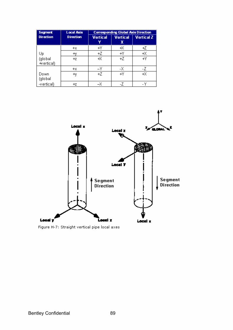
Bentley Confidential 89
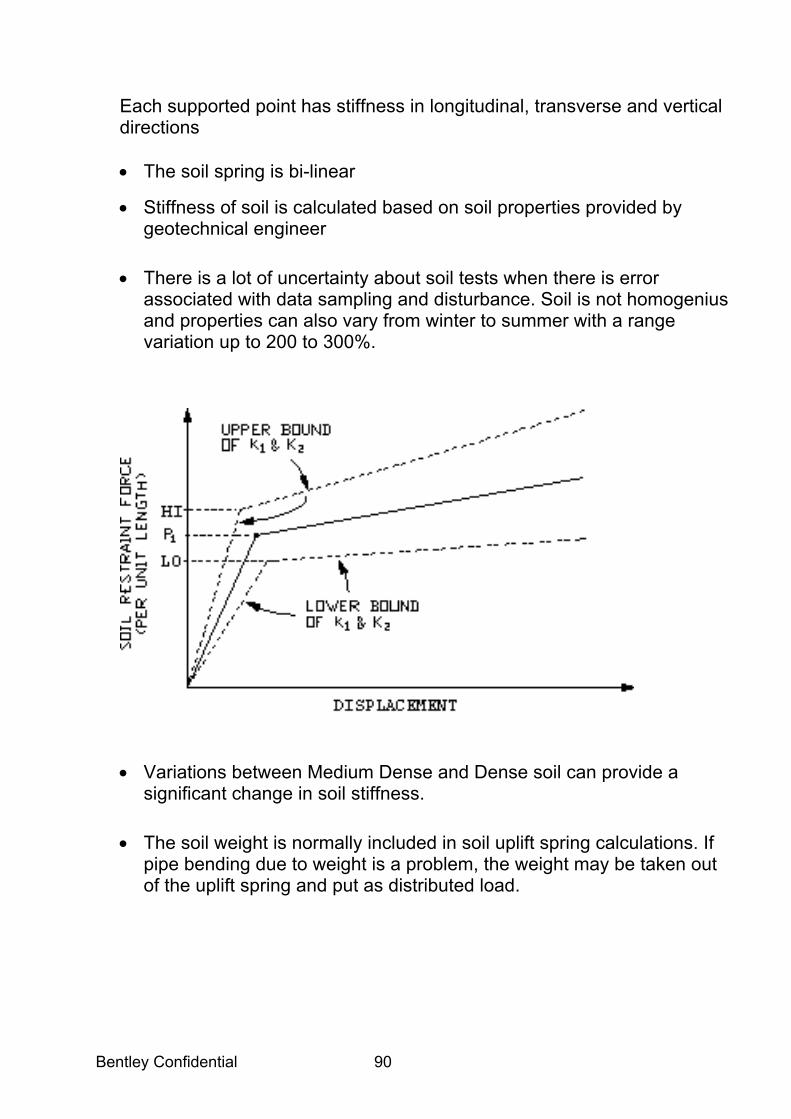
Bentley Confidential 90
Each supported point has stiffness in longitudinal, transverse and vertical directions • The soil spring is bi-linear
• Stiffness of soil is calculated based on soil properties provided by geotechnical engineer
• There is a lot of uncertainty about soil tests when there is error associated with data sampling and disturbance. Soil is not homogenius and properties can also vary from winter to summer with a range variation up to 200 to 300%.
• Variations between Medium Dense and Dense soil can provide a significant change in soil stiffness.
• The soil weight is normally included in soil uplift spring calculations. If pipe bending due to weight is a problem, the weight may be taken out of the uplift spring and put as distributed load.
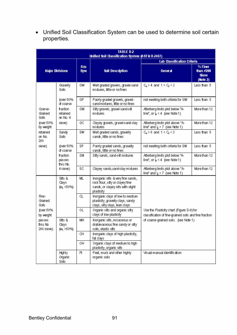
Bentley Confidential 91
• Unified Soil Classification System can be used to determine soil certain properties.
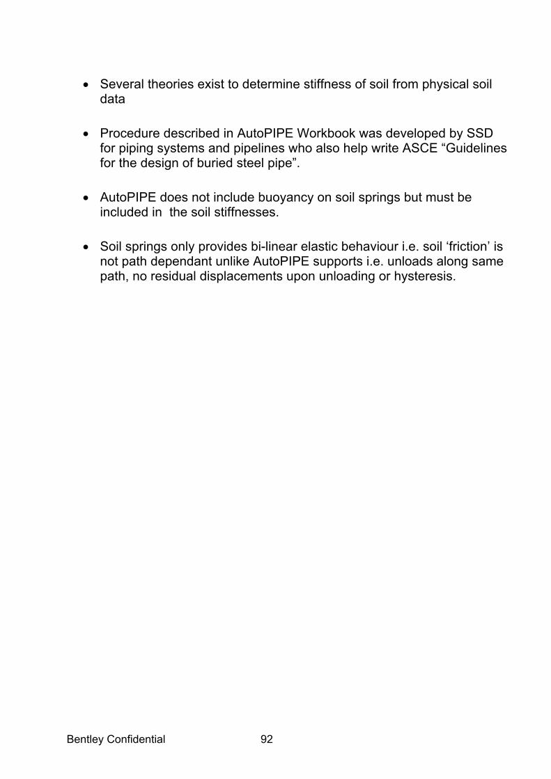
Bentley Confidential 92
• Several theories exist to determine stiffness of soil from physical soil data
• Procedure described in AutoPIPE Workbook was developed by SSD for piping systems and pipelines who also help write ASCE “Guidelines for the design of buried steel pipe”.
• AutoPIPE does not include buoyancy on soil springs but must be included in the soil stiffnesses.
• Soil springs only provides bi-linear elastic behaviour i.e. soil ‘friction’ is not path dependant unlike AutoPIPE supports i.e. unloads along same path, no residual displacements upon unloading or hysteresis.

Bentley Confidential 93
Ground Level
Vertical Pipe with Vertical soil properties.
Buried Pipe with Horizontal soil properties.
Close soil spacing around bends

Bentley Confidential 94
Some Key Design Points:
A) Ensure AutoPIPE soil spacing guidelines in the Reference online Help are followed:

Bentley Confidential
95
Question : My buried piping system is showing large Displacement's in the gravity case? ANSWER. Soil supports are specified for most models with a final stiffness K2 = 0, although AutoPIPE can still solve this problem the results may be invalid if the nonlinear system gives a large deformation. P1 becomes the ultimate soil restraint force for any displacement that is greater than the corresponding yield displacement. The soil should still have some stiffness after yield to restrain the pipe, this is accomplished by specifying a non-zero K2 value (e.g. K2= 0.01) or to include more restraints in the system or reduce the soil span in the soil identifier. Note that may also be possible that the K1 values for the soil are not providing enough stiffness to the system. The value of 0.01 for k2 is arbitrary. It is meant to denote elastic-plastic case. The use of zero could cause instability or unreasonably large displacements. Conversely, if k2 is not zero, large displacements could cause less accurate calculations for the soil restraint force (since there is no cutoff point for the upper end of the k2 region).
Question : How do I model a large sweep bend with radius = 50ft? Answer: Assuming the bend has supports along it then model the bend as series of straight pipe run sections with offsets calculated as a segmented miter bend. Alternatively enter the bend with radius = 50x12 = 600 inches (for ENGLISH units, by overriding the word Long or Short in the radius field. Radius units is displayed in the lower right of the main AutoPIPE window) and insert soil over the large bend with large value of downward soil stiffness, vertical up and lateral stiffness = 0, longitudinal stiffness = 0 (or some nominal value to include some frictional resistance).
Question : How can I simulate soil settlement on part of my piping system? Answer: If the piping system is above ground then at the v-stop and guide supports we recommend to apply settlement displacement in a user case e.g. U1. This will allow the soil settlement to be observed as a unique loading. Then edit the sustained code case combination SUS + Gr to include U1 i.e. the settlement is added to the sustained stresses. If the piping system is buried then the imposed displacement at defined node points (with soil) would give the soil settlement profile. In other words, the base of each soil spring is subject to a displacement interpolated from adjacent nodes with imposed displacements. Hence select the range of points and Insert/xtra data / imposed support displacement = settlement value in the U1 case. To consider settlement for hanger selection, the following is recommended:
Bentley Confidential 96
1. Using model A, add the settlement in the T1 case and run the hanger selection to size the spring. 2. Copy model A to Model B. 3. Using model B, change the settlement from case T1 to case U1 and create user non-code combinations using U1 and add U1 into the sustained stress case GR+MaxP as above. 4. Using a non-code combination e.g. GR+T1+U1 the combined movement and load on the supports including any spring hangers can be evaluated.
Question : My seabed piping shows a large unexpected displacement. Can you please explain. Answer: When the 2nd soil stiffness (K2) is set to zero, the pipe displacement can be large or can cause instability as the soil yields. A perfectly plastic soil K2 = 0 is not typical unless it is called plastic clay. Most soils especially sand have a parabolic force-displacement shape and a larger K2 value is justified but it is conservative to assume a small K2 value. It is advisable with a model so sensitive to changing the K2 value, to examine the soil displacements and forces for more detailed evaluation of yielding e.g. as seen in the soil forces report the horizontal soil force is about 176 kg/m at A78 compared to the P1 value is only 145.8 kg/m hence the soil does not have enough lateral resistance to support this pipe.
Question : Why is my buried piping showing large displacements? Answer: The primary reason for the large displacements is the ultimate soil strength (P1). As seen in the soil forces report the vertical soil force is about 290-A295 lb/ft at A23 to A19 compared to the P1 is only 193.7 lb/ft hence the soil does not have enough resistance to carry this 28" pipe.
Question : How do I model non-embedded and semi-embedded piping? Non-embedded pipe soil stiffness e.g. Seabed piping Answer: The Buried pipe option can be used to model semi-embedded or non-embedded piping. The difficulty is calculating a transverse horizontal(lateral) and longitudinal soil stiffness. a) The vertical up soil stiffness K1, P1 and K2 can be taken as 0. b) The transverse horizontal K1 and P1 is usually taken as low values. c) Transverse vertical down K1 and p1 can be calculated as non-zero with H=0 e.g. eqn D-15 in the appendices under PIPEsoil.

Bentley Confidential
97
d) The longitudinal K1 and P1 would go to zero with Z=0 but there may be an alternative equation in some textbook which would calculate a non-zero longitudinal K1 and P1 although suspect it would be a low value since only assumed line contact of soil with the pipe. You may wish to enter some non-zero K1 and P1 values to evaluate the longitudinal frictional stiffness effect back on the pipe system. Note: Recommend set all final stiffness, K2 = 0.1 lb/in/ft (0.006Kg/m/mm) Semi Embedded pipe soil It sounds like you want to model the seabed piping as semi embedded i.e. all soil stiffnesses with all reasonable calculated values for horizontal pipe (including submerged effect on soil) except vertical up resistance K1, P1 and K2 = 0 Refer to Workbook / Pipe soil transition model for calculating values of soil stiffness.
Question : How do I model subsidence of my buried pipe? Answer: One method to simulate subsidence of known amount e.g. 25mm. Set the yield P1 = 25 as shown below and K1 (initial) value = 0.001 and calculated soil stiffness = K2 (final). SOIL PROPERTIES Soil Initial K yield P Final K Yield disp ID Dirn (N/mm/mm ) (N/m ) (N/mm/mm ) (mm ) ------ ------- ---------- --------- ---------- ---------- SOIL1 Horiz. 6.540 699861.00 0.000 107.0118 Long 17.540 43859.000 0.000 2.5005 Vert Up 2.790 139303.00 0.000 49.9291 Vert Dn 0.001 25.000 23.030 24.9999 If the maximum settlement is unknown, then model the soft waterlogged soil over the known span and known firmer soil at ends. Apply the over-burden sand weight as UDL load or vertical wind load (to simulate the pressure of the 4m sand) on the pipe and observe the deformation and check the resulting maximum slope. All beam theory piping analysis programs such as AutoPIPE, Caesar, pipeplus are based on small deformation theory and large displacements can give an ill-conditioned solution and erroneous results. As a check that AutoPIPE can handle these large deformations use the following rule of thumb. Check that the maximum slope angle in radians of the deformed pipe = approx. sin(slope angle) then the solution should be ok.

Bentley Confidential 98
Question : How do I model soil friction for my buried pipe? Answer: There is no concept of friction for buried pipe. What you enter are stiffness and not friction. You may be able to simulate friction, but that is left to the user ingenuity. The axial soil force of T1=19900 N is correct when the pipe displaces more than 1 mm (y1=P1/K1). As you see that value is the P1 value which the user can set manually.
Question : Can you please provide some references for soil properties. Answer: Guidelines for Design of Buried Steel Pipe. July 2001 published by ASCE references the AutoPIPE program. http://www.americanlifelinesalliance.org/pdf/buried_pipe.pdf ASCE guidelines for design of buried steel pipe Ko = Coeff of earth pressure at rest i.e. ko = 0.4 to 0.5 for Sand ks = Average earth pressure coefficient = (1+ko)/2=(0.7-0.8) [Used by AutoPIPE] where ks = (1+ko)/2
Buried Pipe Design' by Moser. Essence of Soil Mechanics and Foundations : Basic Geotechnics by David F
McCarthy . Publisher : Prentice Hall. Soil Mechanics in Engineering Practice by Karl Terzaghi, Publisher : John Wiley &
Sons
Question : Is an imposed displacement applied to a soil spring? Answer: Technically you need a support where your imposed displacement is. The support should have a component in the direction of imposed displacement. The imposed displacement is actually applied to the base of the spring away from the pipe and that is the reason for the difference. When your support is rigid, the pipe displacement would be the same as the imposed displacement. In case of soil supported piping, the imposed displacement at the nodes would be the soil settlement profile. In other words, the base of each soil spring is subject to a displacement interpolated from adjacent nodes with imposed displacements. You might need to apply imposed displacements at all soil supported node, especially the near and far bend points, if any.
Question : How can I find the load taken by a soil spring? Answer: To resolve a total force (lb) at a straight run point - add a dummy concentrated force = 0 at the pipe point. Perform a static analysis and look at the local forces and moments report as seen below and will see a - and + point, the
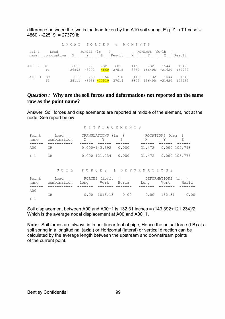
Bentley Confidential
99
difference between the two is the load taken by the A10 soil spring. E.g. Z in T1 case = 4860 - -22519 = 27379 lb L O C A L F O R C E S & M O M E N T S Point Load FORCES (lb ) MOMENTS (ft-lb ) name combination X Y Z Result X Y Z Result ------ ----------- ------ ------ ------ ------ ------- ------- ------- ------- A10 - GR 683 -7 -32 683 116 -32 1544 1549 T1 26895 -3202 4860 27518 3859 156405 -21620 157939 A10 + GR 666 239 -54 710 116 -32 1544 1549 T1 29111 -3936 -22519 37014 3859 156405 -21620 157939
Question : Why are the soil forces and deformations not reported on the same row as the point name?
Answer: Soil forces and displacements are reported at middle of the element, not at the node. See report below: D I S P L A C E M E N T S Point Load TRANSLATIONS (in ) ROTATIONS (deg ) name combination X Y Z X Y Z ------ ----------- ------ ------ ------ ------ ------ ------ A00 GR 0.000-143.392 0.000 31.472 0.000 105.798 + 1 GR 0.000-121.234 0.000 31.472 0.000 105.776 S O I L F O R C E S & D E F O R M A T I O N S Point Load FORCES (lb/ft ) DEFORMATIONS (in ) name combination Long Vert Horiz Long Vert Horiz ------ ----------- ------- ------- ------- ------- ------- ------- A00 GR 0.00 1013.13 0.00 0.00 132.31 0.00 + 1 Soil displacement between A00 and A00+1 is 132.31 inches = (143.392+121.234)/2 Which is the average nodal displacement at A00 and A00+1. Note: Soil forces are always in lb per linear foot of pipe, Hence the actual force (LB) at a soil spring in a longitudinal (axial) or Horizontal (lateral) or vertical direction can be calculated by the average length between the upstream and downstream points of the current point.

Bentley Confidential 100
Question : Why is my buried model unstable? Answer: It appears the horizontal soil yield displacement is very small 0.0012 to 0.004in which would appear to cause local yielding in so many areas for T1 and P1 cases that was unstable. I changed K2 value = 0.1 for all soil identifiers but the model still did not converge in pressure case P1 so I investigated the LOG file and discovered a soil error = 532lb. I searched the log file for 5.32 and found this error at B43 in the P1 vertical case. I removed the soil from B42 to B44 and the P1 case also converged. You could try to tweek the soil properties of 24H78 to also achieve convergence. Note: The log file must be in English units (set input/output units = English).
Question : How can I calculate external soil pressure on the pipe? Answer: The earth pressure can be conservatively estimated from P= SoilDensity * CoverDepth. This is typically ignored under operating load as it is negligible. Effect of surface loads can be estimated and checked independent of other loads since overburden pressure load peaks at the neutral axis of the pipe. Note: Any internal pressure typically reduce the effect of overburden load as it stiffens the pipe. Depending on the requirements of the design specification, the live-load effect may be based on AASHTO HS-20 truck loads, Cooper E-80 railroad loads or a 180 kip airplane gear assembly load. The modified Iowa deflection formula may be used to calculate the pipe ovality under earth and live loads. In steel pipelines, buckling typically occurs when the ovality reaches about 20%. Other construction and code requirements typically limit the amount of permissible cross section ovality for new steel pipelines to much smaller values (e.g., 3% in API RP-1102).

Bentley Confidential
101
Purpose of Piping Codes B31 Codes
• Minimum requirements for safe installation • Guidelines only, not a design handbook • Simplified engineering approach • Allows use of more rigorous analysis.
ASME B&PV Code, Section III
• For nuclear plants • Legal document • Provides mandatory requirements per 10CFR50.55

Bentley Confidential 102
Piping codes ASME Code for Pressure Piping, B31 B31.1 Power Piping (Non nuclear) B31.2 Fuel Gas Piping B31.3 Chemical Plant and Refinery piping B31.4 Liquid Petroleum piping B31.5 Refrigeration piping B31.7 Nuclear Piping (Superseded by ASME Section III) B31.8 Gas Transmission Piping B31.9 Building Service Piping B31.10 Cryogenic Piping B31.11 Slurry Piping ASME Boiler and Pressure Vessel Code, Section III Division 1 Subsection NB Class 1 Components Subsection NC Class 2 Components Subsection ND Class 3 Components European Piping Standards EN13480 EN 13480 (2002) European Standard for Metallic
Industrial Piping

Bentley Confidential
103
Standards and Specification organizations
API American Petroleum Institute ANSI American National Standards Institute ASME American Society of Mechanical Engineers ASTM American Society of Testing and Materials AWS American Welding Society AWWA American Water Works Association MSS Manufacturers Standardization Society of the Valve and
Fitting Industry WRC Welding Research Council CEN European Committee for Standardisation JIS Japanese Standards Association

Bentley Confidential 104
SPECIAL MODELING CASES
1. Hydrotest With Gaps And Friction
2. Exporting Nozzle Loads into WinNOZL
3. Steam Relief Model #2
4. Steam Hammer Model (E.C Goodling)
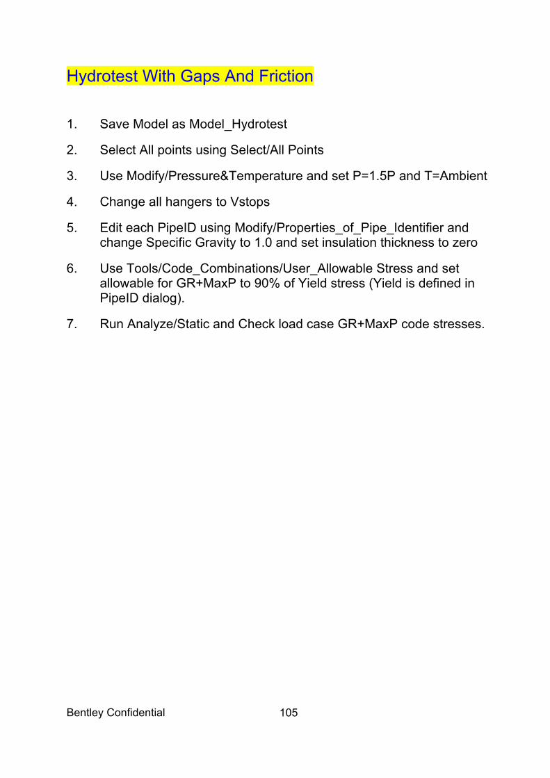
Bentley Confidential
105
Hydrotest With Gaps And Friction
1. Save Model as Model_Hydrotest
2. Select All points using Select/All Points
3. Use Modify/Pressure&Temperature and set P=1.5P and T=Ambient
4. Change all hangers to Vstops
5. Edit each PipeID using Modify/Properties_of_Pipe_Identifier and change Specific Gravity to 1.0 and set insulation thickness to zero
6. Use Tools/Code_Combinations/User_Allowable Stress and set allowable for GR+MaxP to 90% of Yield stress (Yield is defined in PipeID dialog).
7. Run Analyze/Static and Check load case GR+MaxP code stresses.
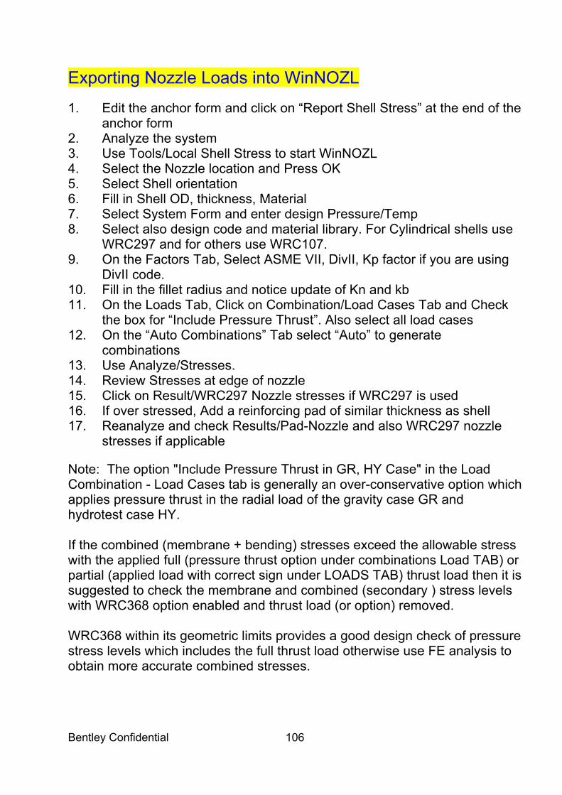
Bentley Confidential 106
Exporting Nozzle Loads into WinNOZL 1. Edit the anchor form and click on “Report Shell Stress” at the end of the
anchor form 2. Analyze the system 3. Use Tools/Local Shell Stress to start WinNOZL 4. Select the Nozzle location and Press OK 5. Select Shell orientation 6. Fill in Shell OD, thickness, Material 7. Select System Form and enter design Pressure/Temp 8. Select also design code and material library. For Cylindrical shells use
WRC297 and for others use WRC107. 9. On the Factors Tab, Select ASME VII, DivII, Kp factor if you are using
DivII code. 10. Fill in the fillet radius and notice update of Kn and kb 11. On the Loads Tab, Click on Combination/Load Cases Tab and Check
the box for “Include Pressure Thrust”. Also select all load cases 12. On the “Auto Combinations” Tab select “Auto” to generate
combinations 13. Use Analyze/Stresses. 14. Review Stresses at edge of nozzle 15. Click on Result/WRC297 Nozzle stresses if WRC297 is used 16. If over stressed, Add a reinforcing pad of similar thickness as shell 17. Reanalyze and check Results/Pad-Nozzle and also WRC297 nozzle
stresses if applicable Note: The option "Include Pressure Thrust in GR, HY Case" in the Load Combination - Load Cases tab is generally an over-conservative option which applies pressure thrust in the radial load of the gravity case GR and hydrotest case HY. If the combined (membrane + bending) stresses exceed the allowable stress with the applied full (pressure thrust option under combinations Load TAB) or partial (applied load with correct sign under LOADS TAB) thrust load then it is suggested to check the membrane and combined (secondary ) stress levels with WRC368 option enabled and thrust load (or option) removed. WRC368 within its geometric limits provides a good design check of pressure stress levels which includes the full thrust load otherwise use FE analysis to obtain more accurate combined stresses.
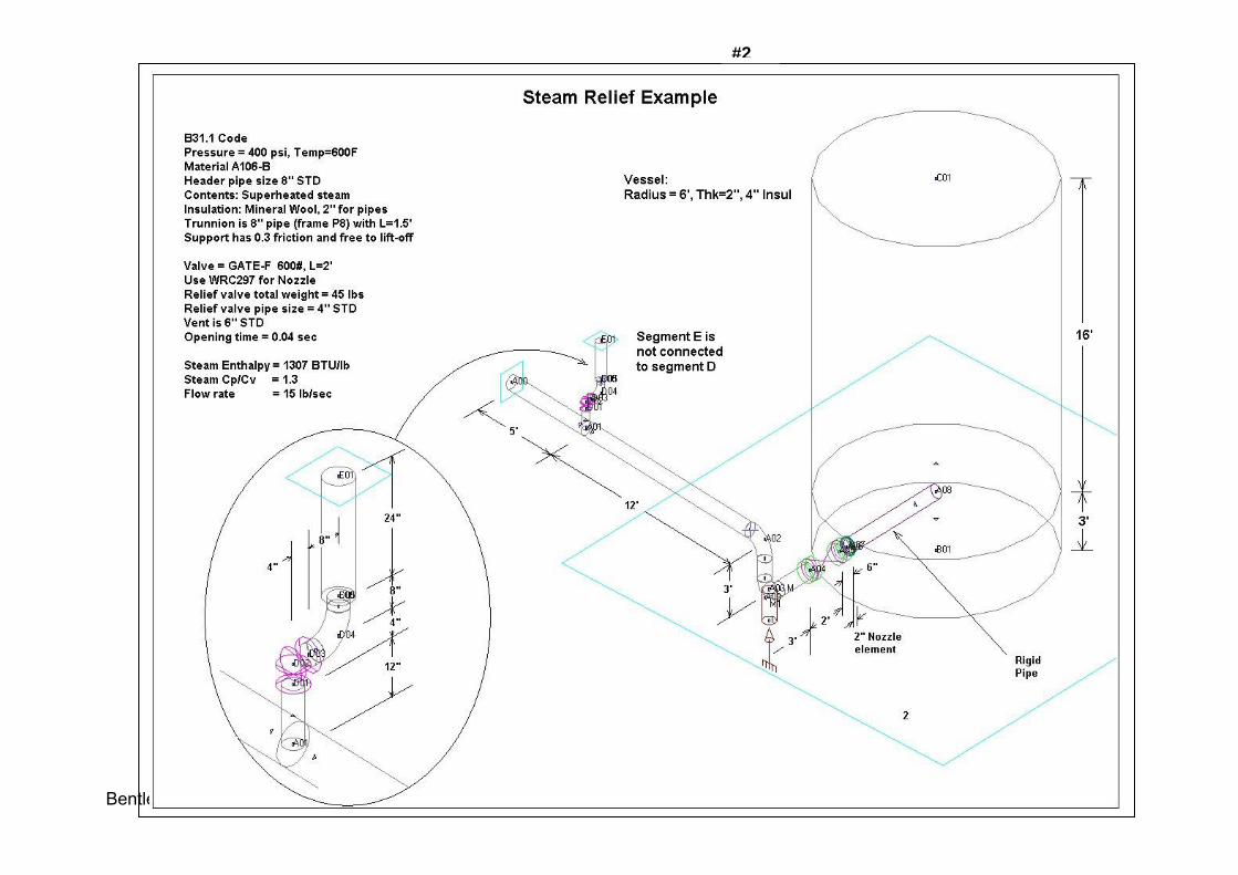
Bentley Confidential
107
#2

Bentley Confidential 108
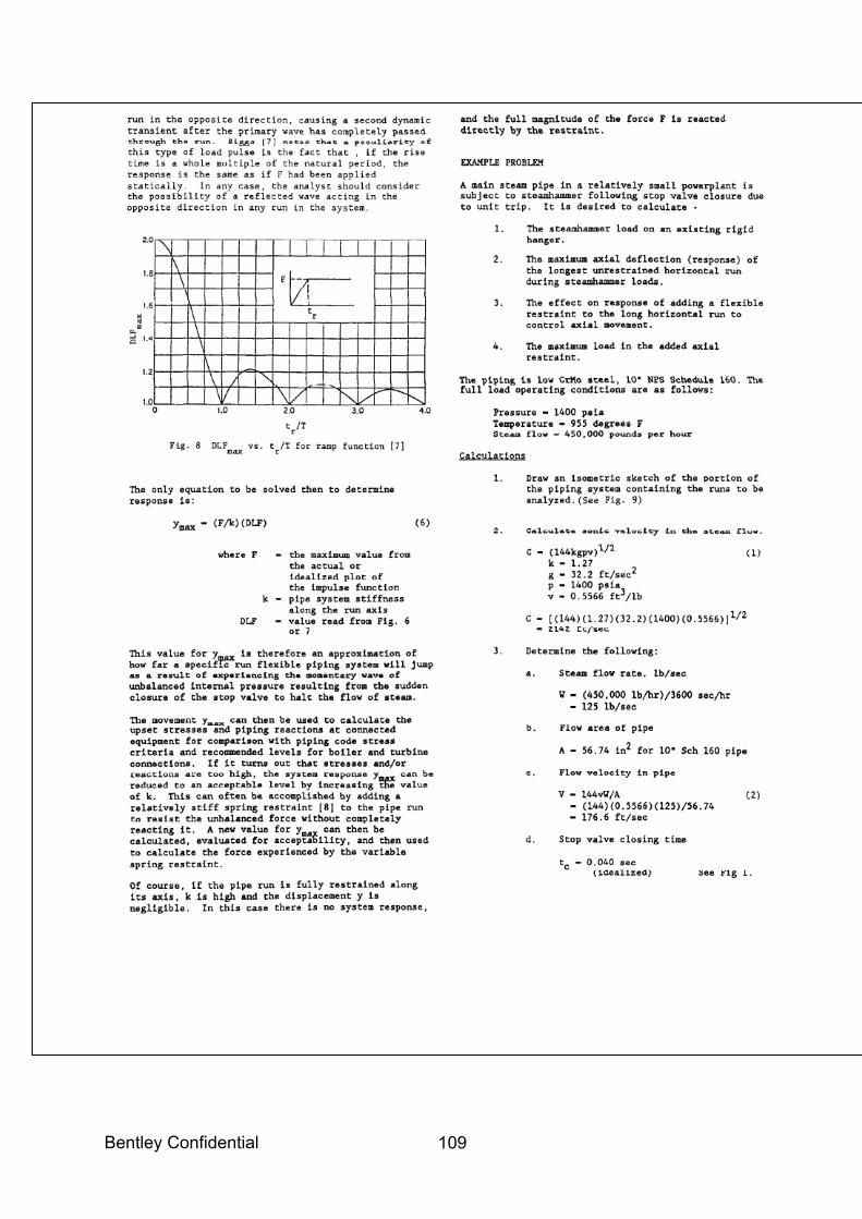
Bentley Confidential
109
Bentley Confidential 110
Bentley Confidential
111
Bentley Confidential 112
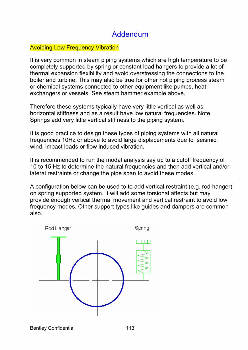
Bentley Confidential
113
Addendum Avoiding Low Frequency Vibration It is very common in steam piping systems which are high temperature to be completely supported by spring or constant load hangers to provide a lot of thermal expansion flexibility and avoid overstressing the connections to the boiler and turbine. This may also be true for other hot piping process steam or chemical systems connected to other equipment like pumps, heat exchangers or vessels. See steam hammer example above. Therefore these systems typically have very little vertical as well as horizontal stiffness and as a result have low natural frequencies. Note: Springs add very little vertical stiffness to the piping system. It is good practice to design these types of piping systems with all natural frequencies 10Hz or above to avoid large displacements due to seismic, wind, impact loads or flow induced vibration. It is recommended to run the modal analysis say up to a cutoff frequency of 10 to 15 Hz to determine the natural frequencies and then add vertical and/or lateral restraints or change the pipe span to avoid these modes. A configuration below can be used to to add vertical restraint (e.g. rod hanger) on spring supported system. It will add some torsional affects but may provide enough vertical thermal movement and vertical restraint to avoid low frequency modes. Other support types like guides and dampers are common also.
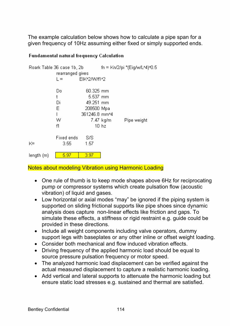
Bentley Confidential 114
The example calculation below shows how to calculate a pipe span for a given frequency of 10Hz assuming either fixed or simply supported ends.
Notes about modeling Vibration using Harmonic Loading
• One rule of thumb is to keep mode shapes above 6Hz for reciprocating pump or compressor systems which create pulsation flow (acoustic vibration) of liquid and gases.
• Low horizontal or axial modes “may” be ignored if the piping system is supported on sliding frictional supports like pipe shoes since dynamic analysis does capture non-linear effects like friction and gaps. To simulate these effects, a stiffness or rigid restraint e.g. guide could be provided in these directions.
• Include all weight components including valve operators, dummy support legs with baseplates or any other inline or offset weight loading.
• Consider both mechanical and flow induced vibration effects. • Driving frequency of the applied harmonic load should be equal to
source pressure pulsation frequency or motor speed. • The analyzed harmonic load displacement can be verified against the
actual measured displacement to capture a realistic harmonic loading. • Add vertical and lateral supports to attenuate the harmonic loading but
ensure static load stresses e.g. sustained and thermal are satisfied.
Bentley Confidential
115
Compressor Vibration using Harmonic Analysis Modeling Problem: An out-of-balance compressor is inducing an oscillating vibration in the attached piping system. This causes concern with the forces, which are produced at the compressor nozzle, and pipe deflections near the compressor. Therefore, it is desired to model the harmonic loads in order to quantify the impact of the vibration on the system. Typically, the pipe/compressor connection point is instrumented, resulting in measurements of the amplitude of motion (Am) and frequency of vibration (fm). In order to accurately solve for piping displacements and the forces exerted on the compressor, it is necessary to determine the harmonic forces, which are induced at the compressor. Then, a harmonic analysis can be performed which produces the desired displacement and pipe force results. NOTE: If there is more than one harmonic vibration source, at other points in the piping system, Steps 1-8 must be applied at each source independently in order to calculate all harmonic forces to be defined in a harmonic load case (HI - H3). However, once the stiffness values have been adjusted at an anchor they do not need to be temporarily set to "rigid" while the other sources are evaluated,
• Step 1: At the anchor, which has been defined to represent the compressor, modify the translational stiffnesses by replacing "rigid" with "0" (zero) for each global coordinate direction, which is a component of . For example, if is observed to act along global X only, then only the "X" DOF is set to zero. However, if is observed to act in a skewed, 3D direction the "X", "Y", and "Z" DOF's should be zeroed.
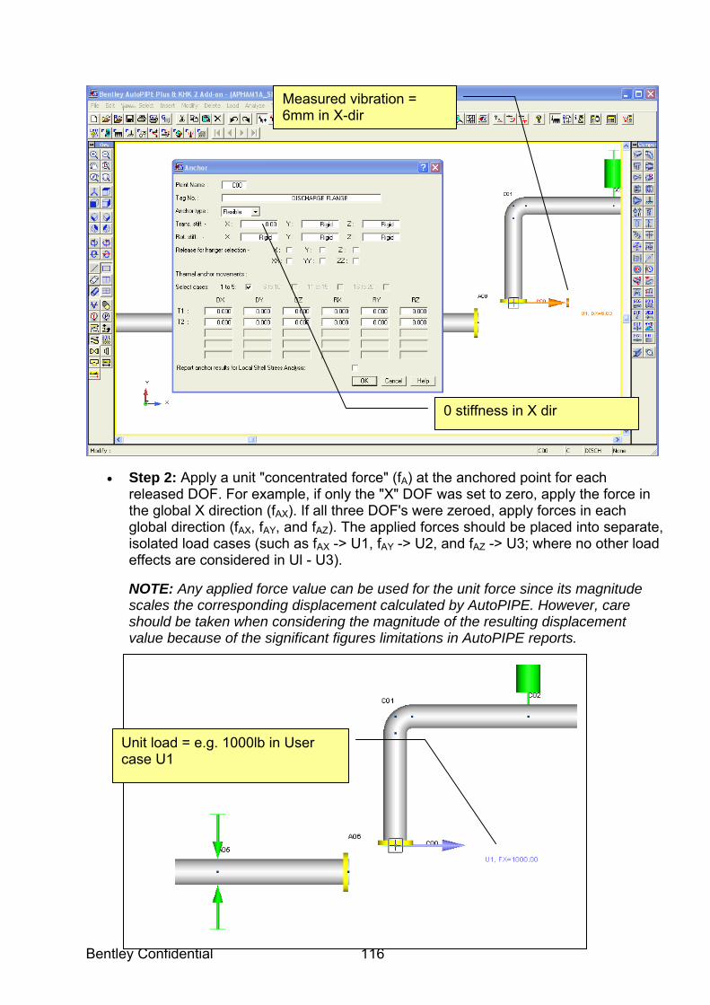
Bentley Confidential 116
• Step 2: Apply a unit "concentrated force" (fA) at the anchored point for each released DOF. For example, if only the "X" DOF was set to zero, apply the force in the global X direction (fAX). If all three DOF's were zeroed, apply forces in each global direction (fAX, fAY, and fAZ). The applied forces should be placed into separate, isolated load cases (such as fAX -> U1, fAY -> U2, and fAZ -> U3; where no other load effects are considered in Ul - U3).
NOTE: Any applied force value can be used for the unit force since its magnitude scales the corresponding displacement calculated by AutoPIPE. However, care should be taken when considering the magnitude of the resulting displacement value because of the significant figures limitations in AutoPIPE reports.
Measured vibration = 6mm in X-dir
0 stiffness in X dir
Unit load = e.g. 1000lb in User case U1
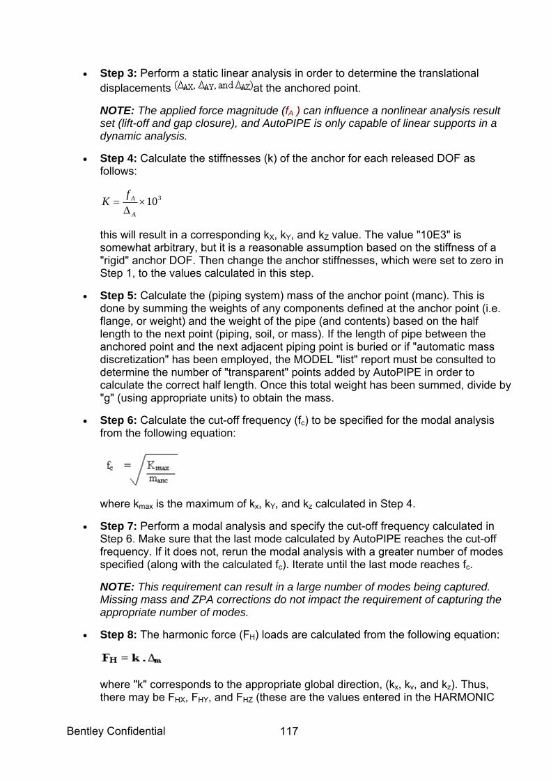
Bentley Confidential
117
• Step 3: Perform a static linear analysis in order to determine the translational displacements at the anchored point.
NOTE: The applied force magnitude (fA ) can influence a nonlinear analysis result set (lift-off and gap closure), and AutoPIPE is only capable of linear supports in a dynamic analysis.
• Step 4: Calculate the stiffnesses (k) of the anchor for each released DOF as follows:
310×∆
=A
AfK
this will result in a corresponding kX, kY, and kZ value. The value "10E3" is somewhat arbitrary, but it is a reasonable assumption based on the stiffness of a "rigid" anchor DOF. Then change the anchor stiffnesses, which were set to zero in Step 1, to the values calculated in this step.
• Step 5: Calculate the (piping system) mass of the anchor point (manc). This is done by summing the weights of any components defined at the anchor point (i.e. flange, or weight) and the weight of the pipe (and contents) based on the half length to the next point (piping, soil, or mass). If the length of pipe between the anchored point and the next adjacent piping point is buried or if "automatic mass discretization" has been employed, the MODEL "list" report must be consulted to determine the number of "transparent" points added by AutoPIPE in order to calculate the correct half length. Once this total weight has been summed, divide by "g" (using appropriate units) to obtain the mass.
• Step 6: Calculate the cut-off frequency (fc) to be specified for the modal analysis from the following equation:
where kmax is the maximum of kx, kY, and kz calculated in Step 4.
• Step 7: Perform a modal analysis and specify the cut-off frequency calculated in Step 6. Make sure that the last mode calculated by AutoPIPE reaches the cut-off frequency. If it does not, rerun the modal analysis with a greater number of modes specified (along with the calculated fc). Iterate until the last mode reaches fc.
NOTE: This requirement can result in a large number of modes being captured. Missing mass and ZPA corrections do not impact the requirement of capturing the appropriate number of modes.
• Step 8: The harmonic force (FH) loads are calculated from the following equation:
where "k" corresponds to the appropriate global direction, (kx, kv, and kz). Thus, there may be FHX, FHY, and FHZ (these are the values entered in the HARMONIC
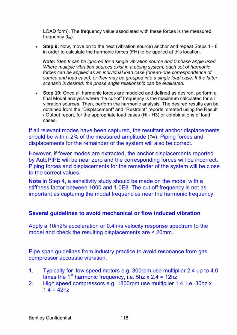
Bentley Confidential 118
LOAD form). The frequency value associated with these forces is the measured frequency (fm).
• Step 9: Now, move on to the next (vibration source) anchor and repeat Steps 1 - 8 in order to calculate the harmonic forces (FH) to be applied at this location.
Note: Step 9 can be ignored for a single vibration source and 0 phase angle used. Where multiple vibration sources exist in a piping system, each set of harmonic forces can be applied as an individual load case (one-to-one correspondence of source and load case), or they may be grouped into a single load case. If the latter scenario is desired, the phase angle relationship can be evaluated.
• Step 10: Once all harmonic forces are modeled and defined as desired, perform a final Modal analysis where the cut-off frequency is the maximum calculated for all vibration sources. Then, perform the harmonic analysis. The desired results can be obtained from the "Displacement" and "Restraint" reports, created using the Result / Output report, for the appropriate load cases (Hi - H3) or combinations of load cases.
If all relevant modes have been captured, the resultant anchor displacements should be within 2% of the measured amplitude ( ). Piping forces and displacements for the remainder of the system will also be correct.
However, if fewer modes are extracted, the anchor displacements reported by AutoPIPE will be near zero and the corresponding forces will be incorrect. Piping forces and displacements for the remainder of the system will be close to the correct values. Note in Step 4, a sensitivity study should be made on the model with a stiffness factor between 1000 and 1.0E8. The cut off frequency is not as important as capturing the modal frequencies near the harmonic frequency. Several guidelines to avoid mechanical or flow induced vibration Apply a 10in2/s acceleration or 0.4in/s velocity response spectrum to the model and check the resulting displacements are < 20mm. Pipe span guidelines from industry practice to avoid resonance from gas compressor accoustic vibration. 1. Typically for low speed motors e.g. 300rpm use multiplier 2.4 up to 4.0
times the 1st harmonic frequency, i.e. 5hz x 2.4 = 12hz 2. High speed compressors e.g. 1800rpm use multiplier 1.4, i.e. 30hz x
1.4 = 42hz
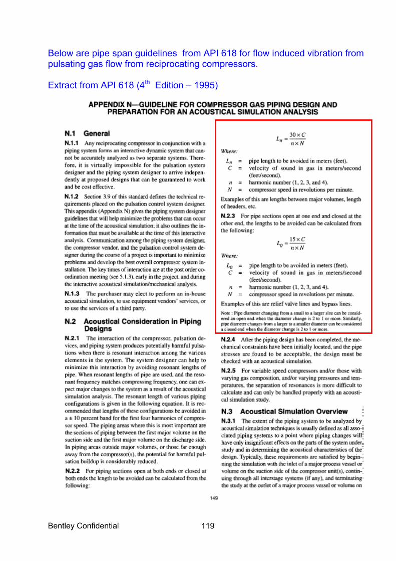
Bentley Confidential
119
Below are pipe span guidelines from API 618 for flow induced vibration from pulsating gas flow from reciprocating compressors. Extract from API 618 (4th Edition – 1995)