Autotuning Sparse Matrix-Vector Multiplication for

Multicore

Jong-Ho ByunRichard LinKatherine A. YelickJames Demmel

Electrical Engineering and Computer SciencesUniversity of California at Berkeley

Technical Report No. UCB/EECS-2012-215

http://www.eecs.berkeley.edu/Pubs/TechRpts/2012/EECS-2012-215.html

November 28, 2012

Copyright © 2012, by the author(s).All rights reserved.

Permission to make digital or hard copies of all or part of this work forpersonal or classroom use is granted without fee provided that copies arenot made or distributed for profit or commercial advantage and that copiesbear this notice and the full citation on the first page. To copy otherwise, torepublish, to post on servers or to redistribute to lists, requires prior specificpermission.

Acknowledgement

Research supported by Microsoft (Award #024263) and Intel (Award#024894) funding and by matching funding by U.C.Discovery (Award#DIG07-10227). Additional support comes from Par Lab affiliates NationalInstruments, Nokia,NVIDIA, Oracle, and Samsung. Also supported by U.S. DOE grants DE-SC0003959, DE-SC0004938, DE-SC0005136, DE-SC0003959, DE-AC02-05-CH11231, DE-FC02-06ER25753, DE-FC02-07ER25799, and DE-FC03-01ER25509.

Autotuning Sparse Matrix-Vector Multiplication for Multicore

Jong-Ho Byun1, Richard Lin1, Katherine Yelick1,2, and James Demmel1,2

1EECS Department, University of California at Berkeley, Berkeley, CA, USA2Lawrence Berkeley National Laboratory, Berkeley, CA, USA

Abstract

Sparse matrix-vector multiplication (SpMV) is an important kernel in scientific and engineering com-puting. Straightforward parallel implementations of SpMV often perform poorly, and with the increasingvariety of architectural features in multicore processors, it is getting more difficult to determine the sparsematrix data structure and corresponding SpMV implementation that optimize performance. In this pa-per we present pOSKI, an autotuning system for SpMV that automatically searches over a large set ofpossible data structures and implementations to optimize SpMV performance on multicore platforms.pOSKI explores a design space that depends on both the nonzero pattern of the sparse matrix, typicallynot known until run-time, and the architecture, which is explored off-line as much as possible, in order toreduce tuning time. We demonstrate significant performance improvements compared to previous serialand parallel implementations, and compare performance to upper bounds based on architectural models.

General Terms: Design, Experimentation, Performance

Additional Key Words and Phrases: Sparse matrix-vector multiplication, Auto-tuning, Multicore.

1 Introduction

Sparse matrix-vector multiplication (SpMV) is an important kernel for a diverse set of applications in manyfields, such as scientific computing, engineering, economic modeling, and information retrieval. Conventionalimplementations of SpMV have historically performed poorly, running at 10% or less of system peak perfor-mance on many uniprocessors, for two major reasons: (1) indirect and irregular memory accesses generallyresult in little spatial or temporal locality, and (2) the speed of accessing index information in the datastructure is limited by memory bandwidth [17, 32, 35, 15]. Since multicore architectures are widely used(starting with dual-core processors in 2001, and now throughout supercomputer, desktop and embeddedcomputing systems), we want to make SpMV as efficient as possible by exploiting multicore’s architecturalfeatures such as the number of cores, simultaneous multithreading, SIMD intrinsics, non-traditional memoryhierarchy including NUMA and shared/private hardware resources [33, 35, 19].

Since SpMV performance depends strongly both on the matrix sparsity pattern and the micro-architecture,optimizing SpMV requires choosing the right combination of data structure and corresponding implementa-tion that best exploit the architecture. This is difficult for two reasons: First, the large variety of sparsitypatterns and architectures, and their complicated interdependencies, make the design space quite large. Sec-ond, since the sparsity pattern is typically not known until run-time, we have to explore this large designspace very quickly. This is in contrast to situations like dense matrix multiplication [4, 33] where off-linetuning is sufficient, so significant time can be spent optimizing. Since the increasing complexity of architec-tures also makes exploring the design space by hand more difficult, we are motivated to develop autotuningsystems that automatically and quickly provide users with optimized SpMV implementations.

The HPC community has been developing autotuning methodologies with empirical search over designspaces of implementations for a variety of important scientific computational kernels, such as linear algebra

1

and signal processing. For examples, ATLAS [33] is a auto-tuning system that implements highly optimizeddense BLAS (basic linear algebra subroutines) and some LAPACK [22] kernels. FFTW [13] and SPIRAL[26] are similar systems for signal processing kernels.

Our work is most closely based on OSKI [32] (Optimized Sparse Kernel Interface), which applies autotun-ing to several sparse linear algebra kernels, including SpMV and sparse triangular solve. OSKI automaticallysearches over the several sparse storage formats and optimizations. The sparse storage formats (see Section2.1 for more details) include CSR, CSC, BCSR and VBR, and the optimizations include register blockingand loop unrolling. Since the nonzero pattern of the sparse matrix is typically not known until run-time,OSKI combines both off-line and run-time tuning. To reduce the run-time tuning costs, OSKI uses a heuris-tic performance model to select the best data structure instead of exhaustive search. However, OSKI onlysupports autotuning for cache-based superscalar uniprocessors, while ATLAS, FFTW and SPIRAL supportautotuning for multicore platforms.

In this paper, we present pOSKI, an autotuning framework for sparse matrix-vector multiplication to achievehigh performance across variety of multicore architectures (the “p” in pOSKI stands for “parallel”). Sinceits predecessor OSKI supports autotuning only for uniprocessors, where the most important optimizationis the data structure with register blocking, we extend OSKI to support an additional set of optimizationsfor diverse multicore platforms. Our new optimizations include the following (see Section 3 for more de-tails): (1) We do off-line autotuning of in-core optimizations for the individual register blocks into whichwe decompose the sparse matrix. These optimizations include SIMD instrinsics, software prefetching andsoftware pipelining, to exploit in-core resources such as private caches, registers and vector instructions. (2)We do run-time autotuning of thread-level parallelism, to optimize parallel efficiency. These optimizationsinclude array padding, thread blocking and NUMA-aware thread mapping, to exploit parallel resources suchas the number of cores, shared caches and memory bandwidth. (3) We reduce the non-trivial tuning cost atrun-time by parallelizing the tuning process, and by using history data, so that prior tuning results can bereused.

We conducted autotuning experiments on three generations of Intel’s multicore architectures (Nehalem,Sandy Bridge-E and Ivy Bridge), and two generations of AMD’s (Santa Rosa and Barcelona), with ten sparsematrices from a wide variety of real applications. Additionally, we compared our measured performance re-sults to SpMV performance bounds on these platforms using the Roofline performance model [34, 36]; thisshows that SpMV is memory bound on all of the platforms and matrices in our test suite. Experimen-tal results show that our autotuning framework improves overall performance by up to 9.3x and 8.6x overthe reference serial SpMV implementation and over OSKI, respectively. We also compare to parallel IntelMKL Sparse BLAS Level 2 routine mkl dcsrmv() and a straightforward OpenMP implementation, gettingspeedups of up to 3.2x over MKL and 8.6x over OpenMP.

The rest of this paper is organized as follows. In section 2 we overview SpMV including sparse matrixstorage formats and the existing auto-tuning system. In section 3 we describe our autotuning frameworkfor SpMV, including our optimizations spaces for both off-line and run-time tuning. In section 4 we presentoverviews of the multicore platforms and sparse matrices in our test suite. In section 5, we present ourexperimental results and analysis comparing to the Roofline performance model, and reference serial andparallel implementations. Finally, we conclude and describe future work in section 6.

2 Background

2.1 Sparse Matrix-Vector Multiplication

Sparse Matrix-Vector Multiplication (SpMV) means computing y = Ax where A is a sparse matrix (i.e. mostentries are zero), and x and y are dense vectors. We refer to x as the source vector and y as the destinationvector. More generally, we also consider y = βy + αAx where α and β are scalars.

2

2.1.1 Data Structures

Sparse matrix data structures generally only store nonzero entries along with additional index information todetermine their locations. There are numerous possible storage formats, with different storage requirements,memory access patterns, and computing characteristics, see [30, 31, 11, 27, 3, 5, 20, 35, 12, 16, 37]. Hereare some examples; for more details see [31]. The simplest sparse format is coordinate (COO) format, whichstores both the row and column indices for each nonzero value. Another widely used format is compressedsparse (CSR) format, which stores matrices row-wise, so the row index does not need to be stored explicitlyas in COO format. The compressed sparse column (CSC) format is similar to CSR, but stores the matrixcolumn-wise. The diagonal (DIAG) format is designed for sparse matrices consisting of some number of(nearly) full nonzero diagonals. Since each diagonal is assumed to be full, we only need to store one indexfor each nonzero diagonal, and no indices for the individual nonzero elements. The ELLPACK/ITPACK(ELL) format is designed for the class of sparse matrices in which most rows have the same number ofnonzeros. If the maximum number of nonzeros in any row is s, then ELL stores the nonzeros values in a 2Darray of size m × s, where m is the number of rows, and a corresponding 2D array of indices. The jaggeddiagonal (JAD) format was designed to overcome the problem of variable length rows/columns by storingthem in decreasing order by the number of nonzeros per row, plus an additional permutation matrix. Theskyline (SKY) format is a composite format which stores the strictly lower triangle of the matrix in CSR,the strictly upper triangle in CSC, and the diagonal in a separate array. The block compressed sparse row(BCSR) format is a further improvement of CSR format by using block structure, to exploit the naturallyoccurring dense block structure typical of matrices arising in finite element method (FEM) simulations ; formore details of BCSR see Section 3.1. The variable block row (VBR) format generalizes the BCSR formatby allowing block rows and columns to have variable sizes.

Comparisons of storage formats are reported in [31, 27, 2, 20]. Vuduc [31] reports that CSR tends tohave the best performance on a wide class of matrices and on a variety of superscalar architectures (SunUltra 2i, Ultra 3, Intel Pentium III, Pentium III-M, Itanium 1 and Itanium 2, IBM Power 3 and Power4), among the basic formats (including CSR, CSC, DIAG, ELL and JAD) considered for SpMV. He alsoreports that BCSR with a proper block size achieves up to 4x speedups over CSR, and VBR shows up to2.1x speedups over CSR. Shahnaz et al. [27] review the several storage formats (including COO, CSR, CSC,JAD, BCSR, and DIAG) for sparse linear systems. They report that COO, CSR and CSC are quite similarto each other with the difference in column and row vector, and CSR has minimal storage requirements.BCSR is useful when the sparse matrix is compressed using square dense blocks of nonzeros in some regularpatterns, however it does not perform significantly better with different block sizes. Bell et al. [2] reportedthe the hybrid format (ELL + COO format) is generally fastest for a broad class of unstructured matrices,comparing among the basic formats (COO, CSR, DIAG, and ELL) on a GPU (GeForce GTX 280); blockstorage formats (BCSR, VBR) are listed as future work. Karakasis et al. [20] conduct a comparative studyand evaluation of block storage formats (including BCSR and VBR formats) for sparse matrices on mul-ticore architectures. They report that one-dimensional VBR provides the best average performance whilethe best storage format depends on a matrix and underlying architecture. They also report that BCSR canprovide more than 50% performance improvement over CSR, but it can lead to more than 70% performancedegradation when selecting improper blocks on a variety of multicore architectures (Intel Hapertown, IntelNehalem and Sun UltraSPARC T2 Niagara2). As demonstrated in this literature, the performance benefitfrom a particular storage format depends strongly on nonzero pattern and underlying micro-architectures.Furthermore, the performance benefit from block storage formats depends on selecting proper block size.

Additionally, to increase the effectiveness of those data structures, reordering rows and columns of matrixcan be used, since this can increase the available block structure. There are numerous reordering algorithmssuch as Column count [14], Approximate Minimum degree (AMD) [1], reverse Cuthill-McKee (RCM) [9],King’s algorithm [21], and the Traveling Salesman Problem (TSP) [25].

3

2.2 OSKI: An autotuning System for SpMV

For sparse matrix computations, OSKI, based in large part on the earlier SPARSITY framework [16, 18],has successfully generated automatically tuned sparse kernels for cache-based superscalar uniprocessors. Thekernels include SpMV and sparse triangular solve (SpTS), among others. OSKI automatically searches overthe several sparse storage formats and optimizations to find the data structure and tuned code that bestexploit properties of both the sparse matrix and the underlying micro-architecture. The sparse storageformats include CSR, CSC, BCSR and VBR, and the optimizations include register blocking and loopunrolling. Since the nonzero pattern of the sparse matrix is not known until run-time, the need for run-time tuning differs from the dense case where only off-line tuning has proved sufficient in practice [4, 33].To reduce cost of run-time tuning, OSKI has two phases, off-line (compile-time) and run-time. The firstphase is an off-line benchmarking phase to characterize the performance of possible implementations onthe given machine. The second is a run-time search consisting of (a) estimating relevant matrix structuralproperties, followed by (b) evaluating a heuristic performance model that combines the estimated propertiesand benchmarking data to select an implementation. The heuristic performance model usually chooses animplementation within 10% of the best implementation found by exhaustive search [31]. However, OSKIonly supports autotuning for cache-based superscalar uniprocessors.

3 pOSKI’s Approach

We extend OSKI’s autotuning framework for SpMV, shown in Figure 1, to support additional optimizationsfor multicore platforms. Our work extends OSKI as follows: (1) We perform off-line autotuning of in-coreoptimizations for performance on individual register blocks. (2) We perform run-time autotuning of thread-level parallelism to optimize parallel efficiency. (3) We reduce the non-trivial tuning cost at run-time byparallelizing the tuning process, and by using history data, so that prior tuning results can be reused. Basedon prior work of our own and others [3, 16, 23, 19, 20, 24, 27, 28, 31, 32, 33, 34, 35, 36], we present theset of the possible optimization strategies for multicore architectures, classified into three areas as shownin Table 1: (1) Data structures, (2) In-core optimizations and (3) Thread-level parallelism. The choiceof data structures depend mostly on the nonzero pattern of the sparse matrix, the in-core optimizationsdepend mostly on single core architectural resources, and the thread-level parallelizations depend mostlyon parallel architectural resources. In this paper we consider only the subset of optimizations which aremarked with an asterisk(∗) in Table 1; implementing the others is future work. Note that low- and high-levelblocking and partitioning also influence the data structure. Array padding is useful to avoid conflict misses.Index compression is useful to reduce memory traffic when it can use fewer bits to store column and rowinformation.

Off-line auto-tuning (search & benchmark)

Run-time auto-tuning (analysis & modeling) +

Figure 1: Overview of autotuning framework for SpMV.

Data structures In-core optimizations Thread-level Parallelism- Storage formats (∗CSR, ∗BCSR, etc.) - Low-level blocking - High-level blocking- Reordering rows and columns - (∗Register, Cache, TLB blocking) - (∗Thread blocking by row blocks)- Index compression - ∗Software pipeline - Other partitioning schemes

- ∗Software prefetching - ∗NUMA-aware mapping- ∗SIMDization - (process and memory afficity)- ∗Loop unrolling - ∗Array padding

1Table 1: Overview of possible SpMV optimizations for multicore architectures. Asterisks (∗) denote theoptimizations considered in this paper.

4

3.1 Block Compressed Sparse Row (BCSR)

We use BCSR storage format for A, because BCSR format can achieve reasonable performance improvementscompared to CSR when the proper register block size is selected, and OSKI’s autotuning heuristic has beenshown to inexpensively select the proper size. We treat each block of BCSR as a dense block, which mayrequire filling in explicit zeros. Register blocks are used to improve register reuse (i.e. locality) by storingas much as possible of the matrix as sequence of small dense blocks, keeping corresponding small blocks ofvector x and y in registers for SpMV. In BCSR format with r × c blocks, an m × n sparse matrix in CSRformat is divided into up to (m/r)× (n/c) blocks, each of size r × c. An example of 2× 2 BCSR format isshown in Figure 2. BCSR format stores only one column index per register block, and one row pointer perblock row starting position in the array of column indices. The memory requirement for BCSR is thereforeO((r × c× k) + (m/r + 1) + (k)), where k is the number of blocks. Thus BCSR format can store fewer rowpointers and column indices than CSR, but at the possible cost of filling in explicit zeros, and so increasingstorage and arithmetic.

0   2   4   5   7  

ptr [m/r +1]

0   3   1   6   4   0   5  

ind [k]

a00   a01   a04  a10   a13   a14   a21   a22   a27  a31   a32   a36  

a44   a45   a54   a55   a60   a61   a66  a71   a75   a76  

val [r×c×k]

a00   a01   a04  

a10   a13   a14  

a21   a22   a27  

a31   a32   a36  

a44   a45  

a54   a55  

a60   a61   a66  

a71   a75   a76  

n

mA =

Figure 2: Example of 2 × 2 BCSR storage format for an 8 × 8 sparse matrix. Nonzero values includingexplicit zeros are stored in the val array. The column index of the (0, 0) entry of each block is stored in indarray. The ptr array points to block row starting positions in the ind array.

3.2 Off-line (compile-time) autotuning

Even though we cannot choose the best register block size until run-time when the input matrix structure isknown, the fastest implementations for all likely r× c block sizes can be selected off-line, by autotuning overa design space of in-core optimizations including loop unrolling, SIMD intrinsics, software prefetching, andsoftware pipelining. Additionally, we can tune over the set of available compilers and compiler optimizationflags.

Our off-line autotuning system performs three major operations as shown in Figure 3: (1) It automati-cally generates codes for various implementations with a set of tunable parameters. The parameters andtheir ranges are shown in Table 2; thus 8 · 8 · 4 · 3 = 768 implementations are generated altogether (notcounting compilers and their flags). (2) It collects benchmarking data for each of these implementationsfor a dense matrix stored in sparse matrix format on each micro-architecture of interest. This can take awhile, but is only done once per architecture and compiler. (3) It selects the best implementation for eachregister block size, storing all the data for later use, including the best observed performance Prc(dense) inMflops/sec for each r×c block size, and all the relevant hardware and software environment parameters (OS,compiler, compiler flags, etc.) needed to make the results reproducible. The benchmark and related dataare stored in .lua files (using the embedded scripting language Lua), and the implementations are stored ina shared object .so file.

Our off-line autotuning is designed to be extensible using a Python-based code generation infrastructure.This leads to more compact and maintainable code in which adding new machine-specific intrinsics forprefetching and SIMD support is straightforward; new architectural concepts like co-processors require a more

5

Generate  HW/OS  configura2on  

Target  HW/OS  pla6orm  

Sample    Dense  Matrix  

1.  Generate  code  variants  

Intrinsics  Set  (Machine-­‐specific)   2.  Benchmark  

code  variants  

Tuning  Space  (s,  r,  c,  d,  imp)   3.  Select  best  implementa2on  

of  variant  (d,  imp)  for  each  data  structure  (s,  r,  c)  

Autotuner (Python)

.so  

.C  .C  .lua  

Installation

Outputs

Generate  benchmark  data  

Transforma2on  Lua  Script  

Figure 3: Off-line autotuning phase. The sample dense matrix is stored in sparse storage format. Thegenerated benchmark data is stored in files (.lua) using Lua, a lightweight embedded scripting language.The selected implementations are compiled based on HW/OS configuration into a shared object (.so).

Tuning Space

Tunable parameter Range of tunable parameter

Storage format (s) s ∈ { CSR, BCSR }Number of rows of register block (r) 1 ≤ r ≤ 8

Number of columns of register block (c) 1 ≤ c ≤ 8∗Software prefetching distance (d) in Bytes d ∈ { 0, 64, 128, 256 }

∗SIMD implementation (imp) imp ∈ { none, SIMDrow, SIMDcol }

Table 2: Tunable parameters for off-line autotuning. Software prefetching distance d = 0 means no prefetch-ing is done. The SIMD implementation denotes the different computation orders to try to facilitate efficientuse of SIMD intrinsics with pipelined and balanced additions and multiplications: SIMDrow indicates arow-wise implementation, and SIMDcol indicates column-wise, and none indicates no intrinsics are used (soit is up to the compiler). All SIMD implementations for each register block are fully unrolled. Choosingd = 0 and imp =none corresponds to the implementation in OSKI. The tunable parameters with asterisks(∗) require the machine-specific intrinsics set.

substantial extension to the code generator, but can still be done in a modular way within the framework.

3.3 Run-time (on-line) autotuning

Run-time autotuning is performed only after the locations of the nonzeros of the sparse are known. Thethree major autotuning steps are shown in Figure 4.

In Step 1, we partition the sparse matrix into submatrices, to be executed by independent threads in theexisting threadpool. As described later, we try to have one thread per core (or more if hyperthreading issupported), accessing a submatrix pinned to the memory most local to that core, i.e. we use a nonuniform-memory access (NUMA) aware mapping. pOSKI currently partitions the matrix into consecutive row blocks(one-dimensional row-wise partitioning) with roughly equal numbers of nonzeros per block, in order tobalance the load. There are many other possible ways to partition into submatrices, such as one-dimensionalcolumn-wise or two-dimensional partitioning schemes with graph or hypergraph partitioning models [7, 8];implementing these is future work.

As discussed in more detail in Section 5, it is not always fastest to use all available cores, so choosingthe optimal number of cores is part of the autotuning problem. Trying all subsets of the available cores atrun-time is too expensive, so doing this tuning well is future work; pOSKI currently just uses all availablecores that are provided. In Section 5 we suggest a natural simple formula for the optimal number of cores,based on measured performance data, but show that it only predicts the right number of cores for some testmatrices and some platforms.

In steps 2 and 3, we need to choose the best data structure and implementation for each submatrix (each

6

submatrix may have a different best choice). Since it is too expensive to exhaustively try all implementationsdescribed in the last section, we use the OSKI heuristic performance model [31, 32] to quickly select the blocksize r × c likely to be fastest (more details below). Alternatively, if the user supplies a “hint” that we coulduse the same data structure and implementation as used before (based on a user-selected matrix name), thiscould more quickly be obtained from a “history database” (a SQLite database .db file). Conversely, tuningresults from using the heuristic performance model can be stored in the database for future use.

Finally each submatrix is copied into its new format. This is often the most expensive autotuning step.All autotuning steps after the matrix is partitioned are performed in parallel by different threads.

1.  Par''on  into  sub-­‐matrices  

2.  Evaluate  Heuris'c  models  for  each  sub-­‐matrix  in  parallel  

3.  Select  the  best  register  block  size  (r,  c)  for  each  sub-­‐

matrix  in  parallel  

Transform  data  structure  for  each  sub-­‐

matrix  in  parallel  

.so  .so  .lua  Sparse  Matrix  

Tuned  matrix  

History  data  

Create  mul'ple  threads  as    a  threadpool  

.so  

Heuristic performance model

Figure 4: Run-time autotuning phase. The outputs of off-line autotuning, benchmark data (.lua) and tunedcodes (.so) are used for run-time autotuning.

Table 3 summarizes the run-time design space. We note that pOSKI currently only implements 1D row-wise partitioning, other partitioning schemes are future work.

Tunable parameters Range of tunable parameters

Partitioning scheme (Thread blocking) 1D row-wise

Storage format (s) s ∈ { CSR, BCSR }Number of rows of register block (r) 1 ≤ r ≤ 8

Number of columns of register block (c) 1 ≤ c ≤ 8

Table 3: Tunable parameters for run-time autotuning.

3.3.1 Thread-level Parallelization

As shown in Figure 4, we first implement a threadpool, reusable multiple threads using thread affinity anda spin lock, based on POSIX Threads (Pthreads) API for thread-level parallelism. We use a first-touchallocation policy to allocate submatrices to the closest DRAM interface to the core that will process them.We also use the affinity routines to pin the each thread to particular core. As mentioned earlier, it is im-portant to use a NUMA-aware mapping to minimize memory access costs. Additionally, our NUMA-awaremapping attempts to maximize usage of multicore resources (from memory bandwidth to physical cores inan architectural hierarchy on a multicore platform) by scaling with the number of threads. This must behandled carefully since the physical core ID depends on the platform. We pad the unit-stride dimension toavoid cache line conflict misses for each sub-matrix.

As mentioned before, so far we only implement a one-dimensional row-wise partitioning scheme, and at-tempt to load balance by approximately equally dividing the number of non-zeros among thread blocks.However, this can result in a load balance problem between submatrices that use different register blocksizes r × c and so run at different speeds. Future work on other partitioning schemes will address thispotential problem.

7

3.3.2 Heuristic performance model

We briefly describe OSKI’s heuristic performance model [31, 32] that we also use to quickly select the optimalregister block size r×c for each submatrix: We choose r and c to maximize the following performance estimatePrc(As) for each sub-matrix As of A:

Prc(As) =Prc(dense)

frc(As)(1)

Here Prc(dense) is the measured performance value (in Mflops/sec) of SpMV for a dense matrix in r × c

BCSR format (from the off-line benchmark data), and frc(As) denotes the estimated fill ratio of As causedby storing explicit zeros in the r × c register blocks:

frc(As) =(number of true nonzeros) + (number of filled in explicit zeros)

number of true nonzeros(2)

frc(As) is estimated cheaply by statistical sampling of As [31, 32].

3.3.3 History data

Despite our use of a heuristic to quickly estimate frc(As), run-time tuning still has a non-trivial cost. Vuduc[31] reported that the total cost of run-time tuning could be at most 43 unblocked SpMV operations on thematrices and platforms in his test suite. Since many users often reuse the same matrix structure in differentruns, this motivates us to quickly reuse previously computed tuning data, by keeping it in a database. Westill have to pay the costs of searching the database (given the matrix name, dimensions, number of nonzeros,and number of submatrices), and converting the matrix from CSR format to the optimized format (storedby the dimensions, number of nonzeros, and optimal r× c for each submatrix). To manage history data, weuse SQLite C/C++ interfaces.

4 Experimental Setup

Before we discuss the measured performance results in the following section, we will briefly summarizecharacteristics of multicore platforms in our test suite, discuss an SpMV performance bound for our multicoreplatforms, and present an overview of the sparse matrices.

4.1 Evaluated multicore platforms

In Table 4, we summarize characteristics of multicore platforms in our test suite, including architecturalconfiguration, system peak performance, and compiler. The system peak performance is for double-precisionfloating point operations, considering neither the max turbo frequency nor AVX, although some of the plat-forms support these techniques. The system peak bandwidth is the peak DRAM memory bandwidth inbillions of bytes transfered per second (GB/s). The system flop:byte ratio is the ratio of the system peakperformance to the system peak bandwidth.

Gainestown (Nehalem) platform is dual-socket quad-core, so 8 cores altogether, with NUMA support.Each core runs at 2.66 GHz, with two hardware threads (hyper threading) to allow simultaneous executionof one 128b SSE multiplier and one 128b SSE adder. The peak double-precision floating point performanceper core is therefore 10.64 GFlops/s, and the system peak double-precision floating point performance is85.12 GFlops/s. Each socket with three fully buffered DDR3-1066 DRAM channels can deliver 21.3 GB/s.The system peak bandwidth is therefore 52.6 GB/s.

Jaketown (Sandy Bridge-E) platform is single-socket six-core. Each core runs at 3.3 GHz, with twohardware threads to allow simultaneous execution of one 128b SSE multiplier and one 128b SSE adder. Thepeak double-precision floating point performance per core is therefore 13.2 GFlops/s, and the system peak

8

Platform Intel AMDGainestown Jaketown Ivy Santarosa Taurus

Core Architecture Nehalem Sandy bridge-E Ivy bridge Santa Rosa BarcelonaModel No. Xeon X5550 Core i7-3960X Core i5-3550 Opteron 2214 Opteron 2356

Core GHz (Max) 2.66 (3.06) 3.3 (3.9) 3.3 (3.7) 2.2 ( - ) 2.3 ( - )# Sockets 2 1 1 2 2

Cores/Socket 4 6 4 2 4HW-threads/Core 2 2 1 1 1

SSE (AVX) 128bit ( - ) 128bit (256bit) 128bit (256bit) 128bit ( - ) 128bit ( - )L1D cache (private) 64KB 32KB 32KB 64KB 64KBL2 cache (private) 256KB 256KB 256KB 1MB 512KBL3 cache (shared) 2× 8MB 15MB 6MB - 2× 2MB

NUMA Yes Yes No Yes YesDRAM Type DDR3-1066 DDR3-1600 DDR3-1600 DDR2-667 DDR2-667

(channels per socket) (3× 64b) (4× 128b) (2× 128b) (1× 128b) (2× 64b)DP GFlops/s 85.12 79.2 26.4 17.6 73.6DRAM GB/s 2× 21.3 2× 25.6 25.6 2× 10.66 2× 10.66

DP flop:byte ratio 2 1.55 1.03 0.83 3.45Compiler icc 12.0.4 icc 12.0.4 icc 12.0.4 gcc 4.3.1 gcc 4.3.2

1Table 4: Overview of evaluated multicore platforms. The Gainestown, Jaketown and Ivy platforms enableeach core to run at max turbo frequency (Max). Each L1D and L2 cache is a private cache per core, andeach L3 cache is a shared cache per socket for all platforms. The system peak performance (DP GFlops/s)is for double-precision floating-point performance. The system peak memory bandwidth (DRAM GB/s) isthe peak DRAM memory bandwidth in GB/s. The system flop:byte ratio (DP flop:byte ratio) is the ratioof the system peak performance to the system peak memory bandwidth for double-precision floating-pointperformance.

double-precision floating point performance is 79.2 GFlops/s. The system peak bandwidth on single-socketwith four fully buffered DDR3-1600 DRAM channels is 51.2 GB/s.

Ivy (Ivy Bridge) platform is single-socket quad-core. Each core runs at 3.3 GHz, win only one hardwarethread with 128b SSE instructions. The peak double-precision floating point performance per core is there-fore 6.6 GFlops/s, and the system peak double-precision floating point performance is 26.4 GFlops/s. Thesystem peak bandwidth on single-socket with two fully buffered DDR3-1600 DRAM channels is 25.6 GB/s.

Santarosa (Santa Rosa) platform is dual-socket dual-core, so 4 cores altogether, with NUMA sup-port. Each core runs at 2.2 GHz, can fetch and decode three x86 instructions per cycle, and executes 6micro-ops per cycle. The each core supports 128b SSE instructions in a half-pumped fashion, with a single64b multiplier datapath and a 64b adder datapath, thus requiring two cycles to execute an SSE packeddouble-precision floating point multiply. The peak double-precision floating point performance per core is4.4 GFlops/s, and the system peak double-precision floating point performance is 17.6 GFlops/s. Each socketwith one fully buffered DDR2-667 DRAM channel can deliver 10.66 GB/s. The system peak bandwidth istherefore 21.33 GB/s.

Taurus (Barcelona) platform is dual-socket quad-core, so 8 cores altogether, with NUMA support.Each core runs at 2.3 GHz, can fetch and decode four x86 instructions per cycle, executes 6 micro-ops percycle, and fully supports 128b SSE instructions. The peak double-precision floating point performance percore is 9.2 GFlops/s, and the system peak double-precision floating point performance is 73.6 GFlops/s.Each socket with two fully buffered DDR2-667 DRAM channels can deliver 10.66 GB/s. The system peakbandwidth is therefore 21.33 GB/s.

9

4.2 Performance predictions

For the expected range of SpMV performance on the above multicore platforms, we adapt the simple rooflineperformance model [36, 34]. In Figure 5, the system peak performance and the system peak bandwidth (blacklines) are derived from the architectural characteristics as shown in Table 4, and the stream bandwidth (bluedashed lines) is the measured memory bandwidth obtained via Stream benchmark [29]. We measure thestream bandwidth with both small and large data sets. The performance of the stream bandwidth withlarge data set can indicate the performance without NUMA support for NUMA architectures (or the peakDP on single core - red lines). The arithmetic intensity is the ratio of compulsory floating-point operations(Flops) to compulsory memory traffic (Bytes) of SpMV. In CSR storage format, SpMV performs 2 × nnzfloating-point operations, and each nonzero is represented by a double-precision value (8-Bytes) and a integercolumn index (4-Bytes), where nnz is the total number of nonzeros. Therefore, each SpMV must read at

atta

inab

le G

FLO

P/s

actual flop:byte ratio

2

4

8

16

32

64

128

1/8 1/4 1/2 1 2 4 8

peak DP

w/out SIMD

mul/add imbalance

w/out ILPpeak syst

em Bandwidth

peak stre

am Bandwidth

w/out NUMA

peak DP on single core

(a) Gainestown platform

atta

inab

le G

FLO

P/s

actual flop:byte ratio

2

4

8

16

32

64

128

1/8 1/4 1/2 1 2 4 8

peak DP

w/out SIMD

mul/add imbalance

w/out ILPpeak s

ystem Bandwidth

peak stre

am Bandwidth

peak DP on single core

large data stream Bandwidth

(b) Jaketown platform

atta

inab

le G

FLO

P/s

actual flop:byte ratio

2

4

8

16

32

64

128

1/8 1/4 1/2 1 2 4 8

peak DP

w/out SIMD

w/out ILPpeak s

ystem Bandwidth

peak stre

am Bandwidth

peak DP on single core

(c) Ivy platform

atta

inab

le G

FLO

P/s

actual flop:byte ratio

2

4

8

16

32

64

128

1/8 1/4 1/2 1 2 4 8

peak DP

w/out SIMD

mul/add imbalance

w/out ILP

peak syst

em Bandwidth

peak stre

am Bandwidth

w/out NUMA

peak DP on single core

(d) Santarosa platform

atta

inab

le G

FLO

P/s

actual flop:byte ratio

2

4

8

16

32

64

128

1/8 1/4 1/2 1 2 4 8

peak DP

w/out SIMD

mul/add imbalance

w/out ILPpeak syst

em Bandwidth

peak stre

am Bandwidth

w/out NUMA

peak DP on single core

(e) Taurus platform

Memory bandwith (GB/s)Performance for SpMV (GFlops/s)

CSR (actual flop:byte ratio = 1/6) BCSR (actual flop:byte ratio = 1/4)

System peak Stream peak System peak Stream peak System peak Stream peaksmall large small large small large

Gainestown 41.6 26.71 12.85 6.93 4.45 2.14 10.40 6.68 3.21Jaketown 51.2 39.79 17.9 8.53 6.63 2.98 12.80 9.95 4.48

Ivy 25.6 19.7 18.71 4.27 3.28 3.12 6.40 4.93 4.68Santarosa 21.33 12.12 6.69 3.56 2.02 1.12 5.33 3.03 1.67Taurus 21.33 16.5 6.9 3.56 2.75 1.15 5.33 4.13 1.73

1(f) Summary of performance model

Figure 5: The roofline performance model of SpMV for our evaluated multicore platforms. The blackline denotes system peak performance bound. The gray dashed line denotes system performance withoutindicated optimizations (SIMD, mul/add imbalance, ILP). The blue dashed line denotes measured streambandwidth. The red dashed line denotes the peak single core performance bound limited by the streambandwidth with a large data set. The green dashed lines denotes bounds of the arithmetic intensity, actualflop:byte ratio, for SpMV. Note the log-log scale.

10

least 12 × nnz bytes. In addition, we assume no cache misses associated with the input/output vectorsand the row pointers of CSR. As a result, SpMV has a compulsory arithmetic intensity less than 2 × nnz/ 12 × nnz, or about 0.166 (leftmost vertical green lines). In BCSR storage format, the register blockingencodes only one column index for each register block. As register blocks can be up to 8× 8, it is possible toamortize this one integer index among many nonzeros, raising the Flop byte ratio from 0.166 to 0.25 whenno explicit zeros are added in BSRC format (shown by the rightmost vertical green lines). By the rooflineperformance model, we expect SpMV to be memory bound on all of our evaluated platforms, since the twovertical green lines intersect the slanted (memory bound) part of the roofline. Thus, we can also expect thatit can achieve the system peak performance of SpMV with fewer cores.

4.3 Sparse matrix test suite

We conduct experiments on sparse matrices from a variety of real applications, including nonlinear opti-mization, power network simulation, and web-connectivity analysis, available from the University of Floridasparse matrix collection [10], as well as a dense matrix stored in sparse matrix storage format. These matri-ces cover a range of properties relevant to SpMV performance, such as overall matrix dimension, non-zerosper row, the existence of dense block substructure, and space required in CSR format. An overview of theircharacteristics appears in Figure 6. Note that Matrix 1 is a dense matrix, and Matrices 2-4 are small matriceswhich might fit into the higher level of caches, and Matrices 5-10 are large matrices. From their densities,we expect that some matrices (Matrices 2, 4, 7, 10) might not benefit from BCSR, while others (Matrices 1,3, 5, 6, 8, 9) might.

Name Spyplot Dimensions ave. nnz/row Space required# Description Nonzeros (nonzero density in CSR formatr = c in {2, 4, 8})

1 Dense1

4K × 4K 4K 144 MBDense matrix in sparse format 16.0M (100, 100, 100)%

2 poisson3Da1

1.3K × 1.3K 230 4 MBComputational fluid dynamics 0.3M (28, 8, 2)%

3 FEM-3D-thremal11

1.7K × 1.7K 235 5 MBThermal problem 0.4M (57, 35, 24)%

4 ns3Da1

20K × 20K 3.6 19 MBComputational fluid dynamic 1.6M (28, 8, 2)%

5 Largebasis1

440K × 440K 11.9 64 MBOptimization problem 5.24M (92, 45, 28)%

6 Tsopf1

35.7K × 35.7K 246 100 MBPower network problem 8.78M (99, 93, 84)%

7 Kkt power1 1

2.06M × 2.06M 6.2 154 MBOptimization problem 12.77M (43, 9, 3)%

8 Ldoor1

952K × 952K 44.6 490 MBStructural problem 42.49M (78, 56, 33)%

9 Bone010 (2D trabecular bone)1

968K × 968K 48.5 552 MBModel reduction problem 47.85M (56, 41, 25)%

10 Wiki-2007 (Wikipedia pages)1

3.56M × 3.56M 12.6 530 MBDirected graph problem 45.4M (26, 7, 2)%

1Figure 6: Overview of sparse matrices used in evaluation study.

5 Experimental Results and Analysis

Here we present our measured SpMV performance on a variety of sparse matrices and multicore platforms.We begin by comparing performance of our off-line autotuning framework to OSKI and the roofline model (ondense matrices in BCSR format). We compare our auto-tuned implementations to reference serial SpMV withCSR, to OSKI, to the parallel Intel MKL Sparse BLAS Level 2 routine, and to a straightforward OpenMP

11

implementation. We also compare our performance to the predicted performance, and finally discuss futurepotential improvements of our autotuning system. Note that we use 8 byte double-precision floating-pointfor matrix and vector values, and 4 byte integers for column indices and row pointers in sparse formats. Allimplementations are compiled with Intel icc on Intel platforms and gcc on AMD platforms with the averageresults shown (average over 50 runs for off-line results and 100 runs for run-time results).

5.1 Off-line (compile-time) autotuning

Here we discuss the performance gain on a single core by our off-line autotuning for SpMV with a densematrix in sparse matrix format, comparing results to OSKI and the roofline model. See Section 3.2 fora discussion of the tuning-parameters and code generation. For all timing measurements, we average theresults over 50 runs.

1 2 3 4 5 6 7 8

1

2

3

4

5

6

7

8

Column

Row

1.74 1.96 2.04 2.09 1.56 1.52 1.49 1.52

1.72 1.93 1.99 2.06 2.09 1.54 1.53 1.53

1.7 1.87 1.96 2.01 2.05 2.09 1.55 1.54

1.66 1.79 1.93 1.98 2.0 2.04 2.06 1.54

1.61 1.74 1.83 1.93 1.94 1.99 2.0 1.97

1.53 1.64 1.72 1.79 1.84 1.89 1.91 1.93

1.39 1.53 1.57 1.61 1.65 1.71 1.74 1.77

1.0 1.16 1.18 1.18 1.19 1.19 1.2 1.2

Gainestown

1000

1250

1500

1750

2000

2250

2500

2750

3000

3250

(a) Gainestown platform

1 2 3 4 5 6 7 8

1

2

3

4

5

6

7

8

Column

Row

1.63 1.85 1.92 1.99 1.75 1.75 1.65 1.73

1.73 1.77 1.87 1.96 2.0 1.69 1.7 1.67

1.72 1.71 1.84 1.91 1.95 1.97 1.72 1.72

1.67 1.64 1.76 1.85 1.91 1.95 1.97 1.69

1.64 1.62 1.67 1.77 1.81 1.88 1.93 1.92

1.56 1.66 1.6 1.64 1.71 1.75 1.78 1.83

1.42 1.58 1.59 1.51 1.54 1.56 1.6 1.61

1.0 1.05 1.07 1.07 1.07 1.08 1.08 1.08

Jaketown

1200

1600

2000

2400

2800

3200

3600

4000

4400

(b) Jaketown platform

1 2 3 4 5 6 7 8

1

2

3

4

5

6

7

8

ColumnR

ow

1.65 1.76 1.8 1.81 1.62 1.6 1.56 1.64

1.69 1.74 1.78 1.81 1.82 1.6 1.6 1.47

1.68 1.7 1.77 1.79 1.8 1.8 1.6 1.54

1.67 1.65 1.73 1.76 1.79 1.8 1.8 1.55

1.62 1.64 1.67 1.72 1.75 1.77 1.78 1.79

1.57 1.63 1.57 1.64 1.69 1.72 1.73 1.75

1.44 1.58 1.6 1.56 1.59 1.61 1.63 1.66

1.0 1.02 1.03 1.03 1.03 1.03 1.03 1.03

Ivy

1200

1600

2000

2400

2800

3200

3600

4000

4400

(c) Ivy platform

1 2 3 4 5 6 7 8

1

2

3

4

5

6

7

8

Column

Row

1.4 1.35 1.16 1.22 1.22 1.3 1.24 1.33

1.38 1.3 1.13 1.12 1.15 1.26 1.27 1.26

1.34 1.3 1.29 1.09 1.14 1.2 1.25 1.22

1.3 1.39 1.33 1.23 1.08 1.08 1.13 1.26

1.29 1.38 1.34 1.2 1.1 1.06 1.1 1.06

1.2 1.27 1.32 1.35 1.24 1.24 1.1 1.12

1.21 1.29 1.29 1.36 1.38 1.41 1.33 1.1

1.0 1.1 1.13 1.22 1.26 1.26 1.3 1.31

Santarosa

200

400

600

800

1000

1200

1400

1600

(d) Santarosa platform

1 2 3 4 5 6 7 8

1

2

3

4

5

6

7

8

Column

Row

1.41 1.38 1.49 1.32 1.43 1.46 1.62 1.52

1.39 1.53 1.22 1.26 1.2 1.35 1.46 1.55

1.39 1.43 1.33 1.24 1.17 1.27 1.36 1.42

1.37 1.51 1.49 1.17 1.14 1.15 1.24 1.33

1.38 1.52 1.52 1.56 0.95 1.02 1.15 1.22

1.35 1.4 1.51 1.51 1.13 1.28 1.15 1.0

1.16 1.43 1.39 1.53 1.5 1.5 1.46 1.66

1.0 1.14 1.19 1.28 1.36 1.32 1.4 1.38

Taurus

200

400

600

800

1000

1200

1400

1600

(e) Taurus platform

Figure 7: SpMV Performance Profiles for OSKI on a dense matrix on a single core. On each platform, eachsquare is an r × c implementation, for 1 ≤ r, c ≤ 8, colored by its performance in MFlops/s, and labeledby its speed up over the reference CSR implementation (r = c = 1). The top of the speed range for eachplatform is the performance bound from the Roofline model, in the last column of Table 5.

5.1.1 OSKI baseline

Figure 7 shows the SpMV performance gain by using BCSR format with register block size r and c com-pared to CSR, for a dense matrix in (B)CSR format. This implementation is the same as OSKI’s (B)CSR

12

implementation, i.e. the code is fully unrolled, but there is no explicit software prefetching or use of SIMD in-trinsics. Each plot in Figure 7 shows all 64 implementations, for 1 ≤ r, c ≤ 8, each colored by its performancein MFlops/s, and labeled by its speedup over the reference CSR implementation (r = c = 1).

OSKI achieves up to 2.1x, 2x, 1.8x, 1.4x and 1.7x speedups over CSR for a dense 4K × 4K matrix onthe Gainestown, Jaketown, Ivy, Santarosa and Taurus platform, respectively. We observe that the peakperformance is near r · c = 36 for Intel’s three platforms, 12 for Santarosa and 16 for Taurus. However, theperformance of register blocks with a single row (r = 1) is not much improved in contrast to taller blocks(r > 1), largely because the register reuse is limited by having a single value of the output vector, resultingin a read-after-write dependency. We also observed that Intel platforms (up to 2.1x speedup over CSR) showslightly better performance gains by register blocking than AMD platforms (up to 1.7x speedup over CSR).

5.1.2 pOSKI’s in-core optimizations

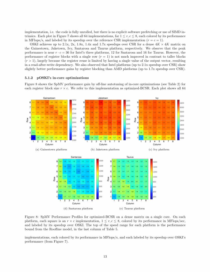
Figure 8 shows the SpMV performance gain by off-line autotuning of in-core optimizations (see Table 2) foreach register block size r × c. We refer to this implementation as optimized-BCSR. Each plot shows all 64

1 2 3 4 5 6 7 8

1

2

3

4

5

6

7

8

Column

Row

1.1 1.0 1.0 1.0 1.2 1.3 1.3 1.2

1.1 1.0 1.0 1.0 1.0 1.3 1.3 1.3

1.1 1.1 1.0 1.0 1.0 1.0 1.3 1.3

1.1 1.0 1.0 1.0 1.0 1.0 1.0 1.3

1.1 1.1 1.1 1.0 1.0 1.0 1.0 1.0

1.1 1.2 1.1 1.1 1.1 1.1 1.0 1.0

1.1 1.2 1.2 1.2 1.1 1.1 1.1 1.1

1.0 1.4 1.4 1.5 1.5 1.5 1.5 1.5

Gainestown

1000

1250

1500

1750

2000

2250

2500

2750

3000

3250

(a) Gainestown platform

1 2 3 4 5 6 7 8

1

2

3

4

5

6

7

8

Column

Row

1.4 1.2 1.1 1.2 1.3 1.3 1.3 1.3

1.3 1.3 1.2 1.2 1.1 1.3 1.3 1.3

1.2 1.3 1.2 1.2 1.1 1.2 1.3 1.3

1.2 1.3 1.2 1.2 1.2 1.2 1.1 1.3

1.2 1.4 1.3 1.3 1.2 1.2 1.1 1.2

1.1 1.3 1.3 1.3 1.2 1.3 1.2 1.2

1.1 1.3 1.3 1.4 1.4 1.4 1.3 1.4

1.1 1.6 1.5 1.7 1.6 1.8 1.7 1.8

Jaketown

1200

1600

2000

2400

2800

3200

3600

4000

4400

(b) Jaketown platform

1 2 3 4 5 6 7 8

1

2

3

4

5

6

7

8

Column

Row

1.1 1.1 1.1 1.1 1.2 1.2 1.2 1.2

1.1 1.1 1.1 1.1 1.0 1.2 1.2 1.3

1.1 1.1 1.1 1.1 1.0 1.1 1.2 1.2

1.1 1.1 1.1 1.1 1.1 1.1 1.0 1.2

1.1 1.1 1.1 1.1 1.1 1.1 1.1 1.1

1.0 1.1 1.2 1.1 1.1 1.1 1.1 1.1

1.0 1.1 1.1 1.2 1.1 1.1 1.1 1.1

1.0 1.5 1.4 1.6 1.5 1.7 1.6 1.7

Ivy

1200

1600

2000

2400

2800

3200

3600

4000

4400

(c) Ivy platform

1 2 3 4 5 6 7 8

1

2

3

4

5

6

7

8

Column

Row

1.4 1.0 1.2 1.2 1.1 1.1 1.1 1.1

1.5 1.0 1.1 1.2 1.1 1.0 1.0 1.1

1.5 1.0 1.0 1.3 1.0 1.1 1.0 1.1

1.5 1.1 1.0 1.1 1.2 1.2 1.1 1.1

1.6 1.5 1.0 1.2 1.2 1.3 1.2 1.3

1.7 1.5 1.3 1.0 1.0 1.0 1.1 1.2

1.4 1.5 1.5 1.5 1.1 1.0 1.0 1.2

1.2 1.7 1.7 1.5 1.5 1.5 1.5 1.5

Santarosa

200

400

600

800

1000

1200

1400

1600

(d) Santarosa platform

1 2 3 4 5 6 7 8

1

2

3

4

5

6

7

8

Column

Row

1.7 1.4 1.2 1.5 1.3 1.4 1.2 1.4

1.8 1.3 1.5 1.7 1.6 1.5 1.3 1.3

1.7 1.5 1.4 1.7 1.6 1.7 1.4 1.4

1.8 1.4 1.2 1.8 1.6 1.8 1.5 1.5

1.7 1.5 1.6 1.3 2.0 2.1 1.7 1.7

1.6 1.6 1.6 1.6 1.6 1.6 1.6 2.0

1.7 1.6 1.7 1.5 1.6 1.4 1.3 1.1

1.5 1.8 1.9 1.8 1.8 1.6 1.6 1.6

Taurus

200

400

600

800

1000

1200

1400

1600

(e) Taurus platform

Figure 8: SpMV Performance Profiles for optimized-BCSR on a dense matrix on a single core. On eachplatform, each square is an r × c implementation, 1 ≤ r, c ≤ 8, colored by its performance in MFlops/sec,and labeled by its speedup over OSKI. The top of the speed range for each platform is the performancebound from the Roofline model, in the last column of Table 5.

implementations, each colored by its performance in MFlops/s, and each labeled by its speedup over OSKI’sperformance (from Figure 7).

13

By autotuning each register block size off-line, optimized-BCSR achieves up to 1.5x, 1.8x, 1.7x, 1.7x and2.1x speedups over OSKI on Gainestown, Jaketown, Ivy, Santrarosa and Taurus, respectively. Althoughthe x86 architectures support hardware prefetching to overcome memory latency from L2 to L1, our useof software prefetching still helps performance by improving locality in L2. For example, we observe onTaurus that optimized-BCSR with r = c = 1 is 1.5x faster than OSKI, by choosing the proper softwareprefetching distance. In-core optimizations are more helpful for blocks with a single row (r = 1) to overcomethe read-after-write dependency problem with a single output. For example, we observe that optimized-BCSR improves the performance up to 90% over OSKI (on Taurus) for register blocks with r = 1. On Intelplatforms the MFlop rate is still slightly lower for blocks with r = 1 than for taller blocks, with r > 1.In contrast, on AMD platforms the performance when r = 1 or c = 1 is often better than for other blocksizes. The automatically selected prefetching distance and SIMDization schemes are shown in Figure 9. Eachplot shows all 64 implementations, each colored by its performance in MFlops/s, and each labeled by itsprefetching distance (upper label) and SIMDization scheme (lower label). In our experience, some decisionsvary from run to run because some choices are very close in performance (see Figure 9(f)).

1 2 3 4 5 6 7 8

1

2

3

4

5

6

7

8

Column

Row

128col

128row

128col

128row

64row

256row

128col

64col

128col

64row

64col

128col

64none

128col

256col

128col

64col

128col

64row

128row

64col

128col

64row

128col

128col

64col

64col

128row

128col

128col

256none

128col

128col

128col

64row

128row

64row

128col

128row

128row

128col

64col

64row

64col

128row

64col

128col

128col

128col

128row

128row

256row

64row

64col

64row

64col

0none

256row

256row

128row

256row

256row

256row

256row

Gainestown

1000

1250

1500

1750

2000

2250

2500

2750

3000

3250

(a) Gainestown platform

1 2 3 4 5 6 7 8

1

2

3

4

5

6

7

8

Column

Row

256col

64row

64row

64row

64row

64row

0row

64col

256col

64col

64row

64row

64row

64row

64row

64col

256col

64col

64row

64row

64row

64row

64row

64row

256col

64col

64row

128row

64row

64col

64row

64row

256col

64row

64row

64row

64row

64row

64col

64col

256col

128row

64col

64col

64row

64col

64row

64col

256col

128row

256col

256row

64row

64col

64row

64row

256none

256row

256row

256row

256row

256row

256row

256row

Jaketown

1200

1600

2000

2400

2800

3200

3600

4000

4400

(b) Jaketown platform

1 2 3 4 5 6 7 8

1

2

3

4

5

6

7

8

Column

Row

256col

64row

64col

64col

64row

64row

64row

128col

256col

128row

64row

64col

64row

64row

64col

64row

64col

64row

64row

0col

64col

64row

64col

64row

128col

64row

64row

64col

64row

0row

64row

64row

256col

64row

64row

64col

64col

64col

64row

64row

64col

64col

64row

64row

64row

64col

64col

64row

128col

64col

64row

64row

64row

64col

64row

64row

256none

128row

256row

256row

128row

256row

256row

256row

Ivy

1200

1600

2000

2400

2800

3200

3600

4000

4400

(c) Ivy platform

1 2 3 4 5 6 7 8

1

2

3

4

5

6

7

8

Column

Row

256col

0col

128row

0row

0row

128row

64col

0row

64col

0none

0row

256col

0row

0row

0row

64col

128col

0row

0none

0col

0row

0row

0row

128row

64col

256col

0none

0row

256col

0row

0row

0row

64col

64row

0none

0row

128row

0col

0row

0row

64col

64row

128row

0col

0none

0none

0row

128row

64col

64col

128row

128col

256row

0none

0none

0col

64none

64row

64row

64row

128row

128row

128row

64row

Santarosa

200

400

600

800

1000

1200

1400

1600

(d) Santarosa platform

1 2 3 4 5 6 7 8

1

2

3

4

5

6

7

8

Column

Row

256col

0row

64row

64row

256row

128row

128row

64row

256col

64row

256row

128row

128row

64row

128row

256row

128col

256col

64row

128row

256row

64row

256row

128row

64col

256col

64row

256col

64row

128row

128row

64row

128col

256col

256row

64row

64row

128col

128row

128row

128col

128row

256row

256col

64row

64row

256row

128col

64col

64row

256row

256row

256row

256col

128row

64row

128none

256row

128row

256row

256row

256row

256row

256row

Taurus

200

400

600

800

1000

1200

1400

1600

(e) Taurus platform

r × c 8× 5 8× 6imp row col row col

d

0 3733 3703 3826 382364 3761 3663 3866 3796128 3522 3432 3600 3634256 3011 3025 3198 3097

r × c 8× 7 8× 8imp row col row col

d

0 3722 3721 3641 366564 3530 3573 3844 3998128 3408 3452 3677 3841256 3110 3066 3185 3174

1(f) Jaketown platform

Figure 9: The selected software prefetching distance (d) and SIMDization scheme (imp) for optimized-BCSRon a dense matrix on a single core. On each platform, each square is an r × c implementation, 1 ≤ r, c ≤ 8,colored by its performance in MFlops/sec, and labeled by its d (upper label in each square) and imp (lowerlabel in each square). Note row indicates SIMDrow (row-wise) and col indicates SIMDcol (column-wise).The top of the speed range for each platform is the performance bound from the Roofline model, in the lastcolumn of Table 5. Figure 9(f) shows examples of possible choices in performance (MFlops/s) on Jaketown.

14

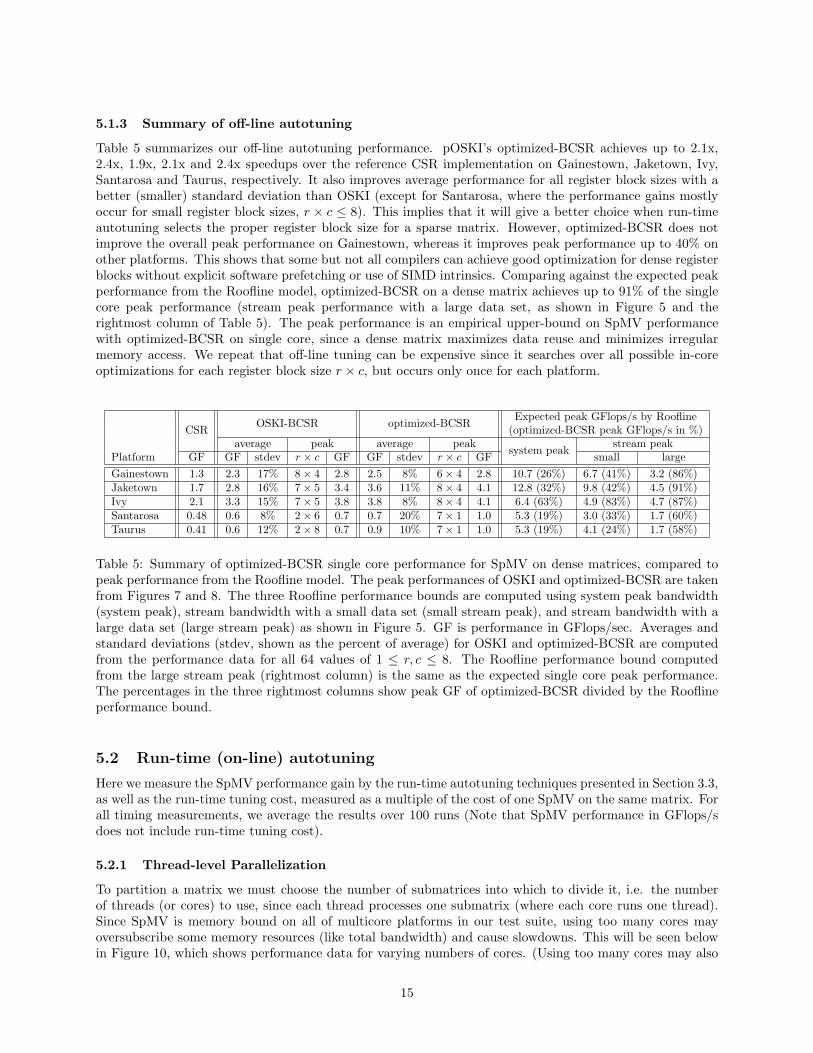
5.1.3 Summary of off-line autotuning

Table 5 summarizes our off-line autotuning performance. pOSKI’s optimized-BCSR achieves up to 2.1x,2.4x, 1.9x, 2.1x and 2.4x speedups over the reference CSR implementation on Gainestown, Jaketown, Ivy,Santarosa and Taurus, respectively. It also improves average performance for all register block sizes with abetter (smaller) standard deviation than OSKI (except for Santarosa, where the performance gains mostlyoccur for small register block sizes, r × c ≤ 8). This implies that it will give a better choice when run-timeautotuning selects the proper register block size for a sparse matrix. However, optimized-BCSR does notimprove the overall peak performance on Gainestown, whereas it improves peak performance up to 40% onother platforms. This shows that some but not all compilers can achieve good optimization for dense registerblocks without explicit software prefetching or use of SIMD intrinsics. Comparing against the expected peakperformance from the Roofline model, optimized-BCSR on a dense matrix achieves up to 91% of the singlecore peak performance (stream peak performance with a large data set, as shown in Figure 5 and therightmost column of Table 5). The peak performance is an empirical upper-bound on SpMV performancewith optimized-BCSR on single core, since a dense matrix maximizes data reuse and minimizes irregularmemory access. We repeat that off-line tuning can be expensive since it searches over all possible in-coreoptimizations for each register block size r × c, but occurs only once for each platform.

CSR OSKI-BCSR optimized-BCSR Expected peak GFlops/s by Roofline(optimized-BCSR peak GFlops/s in %)

average peak average peak system peak stream peakPlatform GF GF stdev r × c GF GF stdev r × c GF small largeGainestown 1.3 2.3 17% 8× 4 2.8 2.5 8% 6× 4 2.8 10.7 (26%) 6.7 (41%) 3.2 (86%)Jaketown 1.7 2.8 16% 7× 5 3.4 3.6 11% 8× 4 4.1 12.8 (32%) 9.8 (42%) 4.5 (91%)Ivy 2.1 3.3 15% 7× 5 3.8 3.8 8% 8× 4 4.1 6.4 (63%) 4.9 (83%) 4.7 (87%)Santarosa 0.48 0.6 8% 2× 6 0.7 0.7 20% 7× 1 1.0 5.3 (19%) 3.0 (33%) 1.7 (60%)Taurus 0.41 0.6 12% 2× 8 0.7 0.9 10% 7× 1 1.0 5.3 (19%) 4.1 (24%) 1.7 (58%)

1Table 5: Summary of optimized-BCSR single core performance for SpMV on dense matrices, compared topeak performance from the Roofline model. The peak performances of OSKI and optimized-BCSR are takenfrom Figures 7 and 8. The three Roofline performance bounds are computed using system peak bandwidth(system peak), stream bandwidth with a small data set (small stream peak), and stream bandwidth with alarge data set (large stream peak) as shown in Figure 5. GF is performance in GFlops/sec. Averages andstandard deviations (stdev, shown as the percent of average) for OSKI and optimized-BCSR are computedfrom the performance data for all 64 values of 1 ≤ r, c ≤ 8. The Roofline performance bound computedfrom the large stream peak (rightmost column) is the same as the expected single core peak performance.The percentages in the three rightmost columns show peak GF of optimized-BCSR divided by the Rooflineperformance bound.

5.2 Run-time (on-line) autotuning

Here we measure the SpMV performance gain by the run-time autotuning techniques presented in Section 3.3,as well as the run-time tuning cost, measured as a multiple of the cost of one SpMV on the same matrix. Forall timing measurements, we average the results over 100 runs (Note that SpMV performance in GFlops/sdoes not include run-time tuning cost).

5.2.1 Thread-level Parallelization

To partition a matrix we must choose the number of submatrices into which to divide it, i.e. the numberof threads (or cores) to use, since each thread processes one submatrix (where each core runs one thread).Since SpMV is memory bound on all of multicore platforms in our test suite, using too many cores mayoversubscribe some memory resources (like total bandwidth) and cause slowdowns. This will be seen belowin Figure 10, which shows performance data for varying numbers of cores. (Using too many cores may also

15

Gainestown

NUMA id 0 1Core id 0 1 2 3 4 5 6 7

HW thread id 0 8 1 9 2 10 3 11 4 12 5 13 6 14 7 15Mapping order 0 8 4 12 2 10 6 14 1 9 5 13 3 11 7 15

Jaketown

Channel id 0 1

-Core id 0 1 2 3 4 5HW thread id 0 1 2 3 4 5 6 7 8 9 10 11

Mapping order 0 6 2 8 4 10 1 7 3 9 5 11

IvyChannel id 0

-Core id 0 1 2 3Mapping order 0 2 1 3

SantarosaNUMA id 0 1

-Core id 0 1 2 3Mapping order 0 2 1 3

TaurusNUMA id 0 1Core id 0 1 2 3 4 5 6 7

Mapping order 0 4 2 6 1 5 3 7

1Table 6: Thread mapping order for efficient thread-level parallelism. NUMA id denotes a group of coreswhich share the NUMA node. Channel id denotes a group of cores which share memory channels. Coreid denotes a group of HW threads (hyperthreading) which share cache. HW thread id denotes a physicalcore (logical processor) id on our platforms. Mapping order denotes our NUMA-aware mapping order whenincreasing the number of threads.

waste energy, a future autotuning topic). After presenting the data, we will suggest a natural simple formulafor the optimal number of cores, based on measured performance data, but show that it only predicts theright number of cores for some test matrices and some platforms; quickly and accurately choosing the optimalnumber of cores remains future work.

Having selected the number of threads, we need to decide how to map each thread to an available core,because not every subset of cores has the same performance: cores may or may not share critical resourceslike cache or memory bandwidth. This is important when we only want to use fewer threads than theavailable number of cores; which cores should we use?

We choose cores using the platform-dependent NUMA-aware mapping shown in Table 6. For example,consider an 8-core Gainestown: The first row, labeled “NUMA id”, divides the 8 cores into two groups of4, according to which fast memory they share. The second row, labeled “core id”, gives a unique numberto each core in each group of 4. The third row, labeled “HW thread id”, give a unique number to each ofthe two hyperthreads that can run on each core, so numbered from 0 to 2 · 8− 1 = 15; the HW thread id isspecified by the Gainestown system. Finally, the last row, labeled “Mapping order”, tells us in what orderto assign submatrices to hyperthreads.

For example, with two submatrices on Gainestown, the first submatrix/thread (Mapping order = 0)pins to the first HW thread (id = 0) in the first NUMA region (id = 0), and the second submatrix/thread(Mapping order = 1) pins to the first HW thread (id = 4) in the second NUMA region (id = 1). This doublesthe total hardware resources available, since each submatrix/thread utilizes 21.3GB/s memory bandwidthof each socket, and the 8MB L3, 256KB L2, and 64KB L1 caches on two 2.66GHz cores, so we would expectthe largest possible speedup. With, say, seven submatrices on Gainestown, we would use hyperthreads fromMapping order = 0 to Mapping order = 6.

Similar scaling behavior for two submatrices/threads is expected for other NUMA platforms (Jaketown,Santarosa and Taurus). Note that Jaketown is a single socket but the two memory channels have NUMAbehavior. However, using two threads on Ivy cannot double memory bandwidth and L3 cache, though theydo double the L2 and L1 caches. Thus, we expect that scaling beyond two threads on Ivy may not help formatrices that do not fit in L2; this is borne out in Figure 10.

Figure 10 shows measured SpMV performance of all our test matrices on all platforms, with differentnumbers of threads. We observe that scaling with two or four threads shows good scalability on mostmatrices (except on Ivy). We also observe that using too many cores degrades the performance in somecases, in particular Gainestown and Jaketown. Finally, for a number of matrices pOSKI’s SpMV exceeds thepeak performance predicted by the Roofline model; this occurs frequently when using the Roofline model

16

with bandwidth measured by the Stream benchmark with a large data set (the lower red dashed lines inFigure 10), and occasionally even using Stream bandwidth with a small data set (the upper red dashedlines). Apparently Stream underestimates the bandwidth of the different memory access patterns accessedby SpMV, and it incurs no data reuse in caches. Also, we recall that small matrices 2 and 3 fit in L3 cacheon Gainestown, Jaketown, and Ivy platforms.

Finally, we describe a simple performance model for predicting the optimal number of threads/subma-trices to use, and compare it to the results in Figure 10: Take the fraction of system peak performanceattained by optimized-BCSR, shown as a percentage in the third column from the right in Table 5; call itx (for example x = 26% for Gainestown). Then ideally using 1/x cores should attain the peak performance

0

1

2

3

4

5

6

7

8

1 2 3 4 5 6 7 8 9 10

Per

form

ance

in G

Flo

ps/s

Matrix

Gainestownstream peak

1 2 4 8 16

(a) Gainestown platform

0 1 2 3 4 5 6 7 8 9

10

1 2 3 4 5 6 7 8 9 10P

erfo

rman

ce in

GF

lops

/s

Matrix

Jaketownstream peak

1 2 4 6 12

(b) Jaketown platform

0

1

2

3

4

5

6

7

1 2 3 4 5 6 7 8 9 10

Per

form

ance

in G

Flo

ps/s

Matrix

Ivystream peak

1 2 4

(c) Ivy platform

0

1

2

3

4

1 2 3 4 5 6 7 8 9 10

Per

form

ance

in G

Flo

ps/s

Matrix

Santarosa

stream peak

1 2 4

(d) Santarosa platform

0

1

2

3

4

5

1 2 3 4 5 6 7 8 9 10

Per

form

ance

in G

Flo

ps/s

Matrix

Taurus

stream peak

1 2 4 8

(e) Taurus platform

0

0.5

1

1.5

2

2.5

1 2 4 8(6) 16(12)

GF

lops

/ s /

Cor

e

Cores

Per-Core Efficiency (Average)

GainestownJaketownIvySantarosaTaurus

(f) Per-core efficiency

Figure 10: The performance of pOSKI on 10 test matrices, on 5 multicore platforms, with varying numbersof cores. Each color on a single matrix denotes the number of threads used to perform SpMV. Two Roofline-based performance bounds are shown, one using bandwidth measured using the Stream benchmark with alarge data set (lower red dashed line) and one with a small data set (upper red dashed line).

17

permitted by the peak system bandwidth on the memory-bound SpMV. Rounding 1/x to the nearest integergive the optimal number of cores as 1/26% ≈ 4 for Gainestown, 1/32% ≈ 3 for Jaketown, 1/63% ≈ 2 forIvy, 1/19% ≈ 5 for Santarosa, and 1/19% ≈ 5 for Taurus. However, comparing to the data in Figure 10, wesee the optimal number of cores is slightly different than expected due to lower per-core efficiency (shownin Figure 10(f)) by scaling with the number of threads; 4, 8 or 16 for Gainestown, 4 or 6 for Jaketown, 4for Ivy, 4 for Santarosa, and 4 or 8 for Taurus. Clearly, a better predictor of the optimal number of cores isneeded by considering other factors, such as memory latency and size of shared caches, which can affect theper-core performance by scaling with the number of threads.

5.2.2 Results from the Heuristic performance model

Run-time autotuning partitions a sparse matrix into submatrices, and then uses the heuristic performancemodel from Section 3.3.2 to select the best data structure and SpMV implementation for each submatrix.Thus, each submatrix may have a different data structure, different SpMV implementation, and differentperformance, possibly upsetting the load balance (improving the load balance is future work).

Table 7 shows in detail the results when we partition a single matrix, Matrix 6 (Tsopf ), into 4 submatrices,for all 5 platforms. For each submatrix and platform, we show (1) the optimal values of the tuning parameters(r, c, d and imp), (2) the expected performance from the heuristic model Prc(As) = Prc(dense)/frc(As), and(3) the measured performance for each submatrix, both running alone on a single core, and while running inparallel with all cores. As can be seen, different optimal parameters may be chosen for different submatriceson the same platform.

Platform Id Tunable parameters Heuristic model GFlops/snnz r × c d imp Prc(dense) frc(As) Prc(As) serial parallel

Gainestown

1 2195751 8× 2 128 row 2.7 1.29 2.09 2.29 1.762 2195456 6× 4 128 row 2.75 1.05 2.62 3.07 2.023 2195798 6× 4 128 row 2.75 1.05 2.62 3.07 2.014 2194944 4× 4 128 row 2.6 1.05 2.48 3.07 2.00

overall 2.83 6.46

Jaketown

1 2195751 8× 4 64 row 4.07 1.39 2.93 2.8 2.202 2195456 8× 4 64 row 4.07 1.07 3.8 3.84 2.363 2195798 8× 4 64 row 4.07 1.07 3.8 3.81 2.404 2194944 5× 4 128 row 3.91 1.05 3.72 3.83 2.37

overall 3.5 8.9

Ivy

1 2195751 8× 2 64 row 4.06 1.29 3.15 3.11 1.052 2195456 7× 2 128 row 3.99 1.05 3.8 3.9 1.103 2195798 8× 2 64 row 4.06 1.05 3.87 3.99 1.104 2194944 7× 2 128 row 3.99 1.05 3.8 3.89 1.10

overall 3.68 4.18

Santarosa

1 2195751 3× 1 64 col 0.96 1.08 0.89 0.86 0.592 2195456 7× 1 64 col 1.00 1.05 0.95 0.97 0.683 2195798 4× 1 64 col 0.99 1.05 0.94 0.96 0.684 2194944 7× 1 64 col 1.00 1.05 0.95 0.96 0.69

overall 0.98 2.39

Taurus

1 2195751 2× 2 64 row 0.95 1.05 0.90 0.85 0.712 2195456 5× 1 64 col 1.00 1.05 0.95 1.02 0.593 2195798 5× 1 64 col 1.00 1.04 0.96 1.06 0.714 2194944 5× 1 64 col 1.00 1.04 0.96 1.07 0.59

overall 0.92 2.92

1Table 7: Example of the selected tuning parameters with 4 threads for Matrix 6 (Tsopf). Id denotes thesubmatrix, nnz is the number of non-zeros for each submatrix, r × c is the selected block size, d is theselected software prefetching distance, imp is the selected SIMD implementation, Prc(dense) is measuredSpMV performance for a dense matrix with r × c, frc(As) is the fill ratio, Prc(As) is the expected SpMVperformance, and GFlops/s is the measured per-core performance in serial and in parallel.

18

First, to confirm the accuracy of the heuristic model, we compare the measured serial performance(second to last column of Table 7) with the predicted performance (third to last column, Prc(As)); thereis reasonable agreement, with some over- and some underestimates. Second, to understand the impactof parallelism, we compare the measured per-core performance in the last column to the measure serialperformance; performance drops, sometimes significantly, because of resource conflicts. In particular, itdrops almost 4x on Ivy, because 1 core is enough to saturate the memory bandwidth for this matrix.

5.2.3 Run-time tuning cost

The cost of run-time tuning depends on whether we use our history database or not: If we do not use it, weneed to apply the heuristic performance model to choose the optimal data structure and implementation. Ifwe do use it, we incur the (lesser) cost of accessing the database. Either way, we pay the cost of copying theinput matrix from CSR format to the optimal format.

Figure 11 shows the run-time tuning costs in three cases, measured as a multiple of the time to perform asingle sequential SpMV on the matrix in CSR format (i.e. without optimizations): (1) Case-I: autotuningwith the heuristic performance model in serial, (2) Case-II: autotuning with the heuristic performance modelin parallel, and (3) Case-III: autotuning with the history database in parallel. In Cases II and III, the numberof cores is the optimal number as shown in Figure 10.

The dense matrix in sparse format (Matrix 1) is special case we discuss separately. We also consider thesmaller matrices (Matrices 2-4) separately from the larger ones (Matrices 5-10), because the short runningtime for the small matrices makes the relative cost of tuning much more expensive.

1  

10  

100  

1000  

1   2   3   4   5   6   7   8   9   10  

Tuning  cost  /  SpM

V  

Matrix  

Gainestown  Case-­‐I  Case-­‐II  Case-­‐III  

(a) Gainestown platform

1  

10  

100  

1000  

1   2   3   4   5   6   7   8   9   10  

Tuning  cost  /  SpM

V  

Matrix  

Jaketown  Case-­‐I  Case-­‐II  Case-­‐III  

(b) Jaketown platform

1  

10  

100  

1000  

1   2   3   4   5   6   7   8   9   10  

Tuning  cost  /  SpM

V  

Matrix  

Ivy  Case-­‐I  Case-­‐II  Case-­‐III  

(c) Ivy platform

1  

10  

100  

1000  

1   2   3   4   5   6   7   8   9   10  

Tuning  cost  /  SpM

V  

Matrix  

Santarosa  Case-­‐I  Case-­‐II  Case-­‐III  

(d) Santarosa platform

1  

10  

100  

1000  

1   2   3   4   5   6   7   8   9   10  

Tuning  cost  /  SpM

V  

Matrix  

Taurus  Case-­‐I  Case-­‐II  Case-­‐III  

(e) Taurus platform

Figure 11: The run-time autotuning cost, relative to unoptimized SpMV in CSR format. Case-I denotesautotuning with the heuristic model in serial. Case-II denotes autotuning with the heuristic model in parallel.Case-III denotes autotuning with history data in parallel. Note that the vertical axises are log-scale.

19

We see that for a dense matrix (Matrix 1) and for all platforms, the average run-time tuning cost is 113,143 and 160 unoptimized SpMVs in Case I, II and III, respectively. Case-II costs 1.7x, 1.0x and 1.3x lessthan Case-I on Gainestown, Santarosa and Taurus, however, it costs 1.3x and 1.3x more than Case-I onJaketown and Ivy. Case-III costs 5.2x, 1.1x, 1.1x and 1.4x less than Case-I on Gainestown, Jaketown, Ivyand Santarosa, respectively, however, it costs 1.8x more than Case-I on Taurus.

We see that for small matrices (Matrices 2-4) and for all platforms, the average run-time tuning cost is179, 201 and 300 unoptimized SpMVs in Case I, II and III, respectively. Case-II costs up to 1.1x, 1.2x, 1.2x,1.8x and 1.8x less than Case-I on Gainestown, Jaketown, Ivy, Santarosa and Taurus, respectively. However,for a few matrices, Case-II costs at most 1.3x, 1.4x and 1.1x more than Case-I on Gainestown, Jaketown andIvy. Case-III costs up to 1.2x and 2.4x less than Case-I on Jaketown and Ivy. However, for a few matrices, itcosts at most 1.4x, 1.4x, 1.8x and 1.8x more than Case-I on Gainestown, Jaketown, Santarosa and Taurus,respectively.

We see that for large matrices (Matrices 5-10) and for all platforms, the average run-time tuning cost is39, 26 and 14 unoptimized SpMVs in Cases I, II and III, respectively. Case-II costs up to 1.9x, 2x, 1.8x, 2.9xand 5.0x (average 1.5x, 1.6x, 1.5x, 2.2x and 2.7x) less than Case-I on Gainestown, Jaketown, Ivy, Santarosaand Taurus, respectively. However, for a few matrices, it costs at most 1.2x and 1.1x more than Case-I onGainestown and Jaketown. Case-III costs up to 8.2x, 7.4x, 9.5x, 8.2x, and 10.5x (average 4.5x, 4.2x, 4.9x,3.9x and 4.3x) less than Case-I on Gainestown, Jaketown, Ivy, Santarosa and Taurus, respectively.

We observe that parallel tuning (Case-II) and using history data (Case-III) give larger speedups (lessrun-time tuning cost) than Case-I on the largest sparse matrices (Matrices 8-10). However, we also observethat parallel tuning (Case-II) or using history data (Case-III) can result in more cost than Case-I on somecases (specially on small matrices). Further reducing run-time tuning costs is also future work.

5.2.4 Summary of run-time autotuning

For clarity, we present the overall performance of each autotuning optimization condensed into a stacked barformat as seen in Figure 12, in order to see the contribution made by each optimization. We also include theperformance of parallel Intel MKL Sparse BLAS Level 2 routine mkl dcsrmv() and straightforward parallelimplementation with OpenMP and CSR for comparison.

The colored bars have the following meanings. The bottommost, dark green, bar (labeled CSR) indicatesthe performance of the naive implementation, i.e. serial CSR. The second, dark blue, bar (labeled OSKI)indicates the performance of OSKI, i.e. serial performance using OSKI’s optimization (register blocking).The third, light green, bar (labeled SIMD) indicates the performance of optimized-BCSR, i.e. serial per-formance using pOSKI’s in-core optimizations (register blocking, software prefetching and SIMD intrinsics).The fourth, light blue, bar (labeled TB) shows the performance of thread blocking, running in parallel withthe optimal number of cores shown in Figure 10, but without NUMA-aware mapping (pinning threads tocores by OS scheduler). Finally, the topmost, yellow-green, bar (labeled NUMA) indicates the performance ofpOSKI with all of pOSKI’s optimizations including NUMA-aware mapping, again running with the optimalnumber of cores. In addition, we compare our autotuning SpMV performance to the performance boundsfrom the Roofline model as in Figure 10 (dashed red lines).

In Figure 12, some matrices (Matrices 2, 4, 7, 10) do not or slightly improve performance by optimized-BCSR (labeled SIMD), since the matrices are too sparse. Although other matrices (Matrices 3, 5, 6, 8, 9)do get benefits from optimized-BCSR, the gains are less than in the dense matrix (Matrix 1) mainly dueto overheads from filling in explicit zeros within each register block and irregular memory accesses of theinput vector between register blocks. This further suggests that reordering methods for creating larger denseblocks will be worthwhile for optimized-BCSR for other sparse matrices.

All matrices (Matrices 1 to 10) show performance improvement by thread blocking (labeled TB) on allplatforms. Ivy shows the least performance improvement (4% over optimized-BCSR) by thread blocking onLargebasis (Matrix 5). NUMA-aware mapping (labeled NUMA) improves some matrices on NUMA archi-tectures, however it also depends on the matrix and the underlying architecture.

As seen in Figure 12, the overall our autotuning for SpMV for the dense matrix (Matrix 1) in sparse

20

0

1

2

3

4

5

6

7

8

1 2 3 4 5 6 7 8 9 10

Per

form

ance

in G

Flo

ps/s

Matrix

Gainestownstream peak

CSROSKI

SIMDTB

NUMAMKL

OpenMP

(a) Gainestown

0 1 2 3 4 5 6 7 8 9

10

1 2 3 4 5 6 7 8 9 10

Per

form

ance

in G

Flo

ps/s

Matrix

Jaketownstream peak

CSROSKI

SIMDTB

NUMAMKL

OpenMP

(b) Jaketown

0

1

2

3

4

5

6

7

1 2 3 4 5 6 7 8 9 10

Per

form

ance

in G

Flo

ps/s

Matrix

Ivystream peak

CSROSKI

SIMDTB

NUMAMKL

OpenMP

(c) Ivy

0

1

2

3

4

1 2 3 4 5 6 7 8 9 10

Per

form

ance

in G

Flo

ps/s

Matrix

Santarosa

stream peak

CSROSKI

SIMDTB

NUMAOpenMP

(d) Santarosa

0

1

2

3

4

5

1 2 3 4 5 6 7 8 9 10

Per

form

ance

in G

Flo

ps/s

Matrix

Taurus

stream peak

CSROSKI

SIMDTB

NUMAOpenMP

(e) Taurus

pOSKI speedup overCSR OSKI OpenMP MKL

Dense min 2.3 1.3 1.2 1.1Matrix ave 6.6 3.4 4.3 1.8

1 max 9.3 5.5 8.3 3Small min 2 2 0.8 0.7

Matrices ave 5.2 4.8 3.2 12-4 max 9 8.6 8.1 1.3

Large min 1.5 1.1 0.9 0.9Matrices ave 4.3 3.3 2.7 1.6

5-10 max 7.5 5.5 7.4 3.2

Allmin 1.5 1.1 0.8 0.7ave 4.8 3.7 3.0 1.4max 9.3 8.6 8.3 3.2

1(f) Speedups on all platforms

Figure 12: Overall performance of autotuned SpMV. Each colored bar corresponds to performance from adifferent set of optimizations, as described in the text. Intel MKL results on Intel platforms are denoted byblack triangles. OpenMP results are denoted by red circles. Two Roofline-based performance bounds areshown, one using bandwidth measured using the Stream benchmark with a large data set (lower red dashedline) and one with a small data set (upper red dashed line). Minimum, average and maximum speedups foreach subset of matrices are shown in Figure 12(f). Note that speedup less than 1 means slowdown factor.

format achieves up to 74%, 80%, 73%, 57% and 64% of the system peak performance of SpMV (the third-from-rightmost column of the table in Figure 5(f)), and up to 118%, 104%, 95%, 100% and 83% of the

21

Roofline-based performance bound using bandwidth measured with the Stream benchmark with a smalldata set (upper red line) on Gainestown, Jaketown, Ivy, Santarosa and Taurus platform, respectively. Sincethe dense matrix (Matrix 1) in sparse format contains clear dense structure and large dimensions, the overallperformance on the dense matrix is a kind of empirical upper bound on large matrices (Matrix 5-10).

Among large sparse matrices (Matrices 5-10) in our test suite, Tsopf (Matrix 6) shows the highest per-formance on all platforms because it has the highest density, the highest number of nonzeros per rows andthe smallest dimensions (see Figure 6) among Matrices 5-10. Tsopf achieves at least 80% of the performancewith the dense matrix. Wiki-2007 (Matrix 10) shows the lowest performance on all platforms because thematrix is very sparse with the largest dimensions resulting in poor cache locality of input vector. Wiki-2007shows less than 20% of the performance with the dense matrix. Cache and TLB blocking optimizations mayimprove data reuse for large dimensional matrices.

As shown in Figure 12(f), for the dense matrix (Matrix 1) and for all platforms, pOSKI is up to 9.3xfaster than the reference serial CSR implementation, up to 5.5x faster than the optimized serial OSKI imple-mentation, up to 8.3x faster than a straightforward parallel implementation using OpenMP and CSR, andup to 3x faster than the parallel Intel MKL implementation.

For the small matrices (Matrices 2-4) and for all platforms, pOSKI is up to 9x faster than the referenceserial CSR implementation, up to 8.6x faster than the optimized serial OSKI implementation, up to 8.1xfaster than a straightforward parallel implementation using OpenMP and CSR, and up to 1.3x faster thanthe parallel Intel MKL implementation. However, for a few matrices, pOSKI performs at most 1.3x and 1.2xslower than Intel MKL and OpenMP implementations, respectively.

For the large matrices (Matrices 5-10) and for all platforms, pOSKI is up to 7.5x faster than the referenceserial CSR implementation, up to 5.5x faster than the optimized serial OSKI implementation, up to 7.4xfaster than a straightforward parallel implementation using OpenMP and CSR, and up to 3.2x faster thanthe parallel Intel MKL implementation. However, for a few matrices, pOSKI performs at most 1.1x and 1.1xslower than Intel MKL and OpenMP implementations, respectively.

In summary for each platform, pOSKI achieves up to 6.6x, 6.1x, 4.5x, 9.3x and 9x speedups over naiveCSR, up to 6.6x, 4.9x, 3.7x, 4.9x and 8.6x speedups over OSKI, and up to 2.8x, 2.4x, 1.4x, 6.6x and 8.3xspeedups over OpenMP+CSR on Gainestown, Jaketown, Ivy, Santarosa and Taurus, respectively. It achievesup to 3.2x, 1.6x and 1.4x speedups over MKL on Gainestown, Jaketown and Ivy platform, respectively. Ad-ditionally, pOSKI shows better performance than MKL or OpenMP implementations on most cases (42 outof 50 cases), while MKL or OpenMP implementations show better performance than on a few cases (Matrix2 and 3 on Gainestown, Matrix 3-5 on Jaketown, Matrix 4, 5 and 7 on Ivy platform).

6 Conclusions

We have presented pOKSI, an autotuning framework for Sparse Matrix-Vector Multiplication (SpMV) on adiverse set of multicore platforms. We demonstrate significant performance gains over prior implementations:pOSKI is up to 9.3x faster than the reference serial CSR implementation, up to 8.6x faster than the optimizedserial OSKI implementation, up to 8.3x faster than a straightforward parallel implementation using OpenMPand CSR, and up to 3.2x faster than the parallel Intel MKL implementation. However, for a few matrices,pOSKI performs at most 1.3x and 1.2x slower than Intel MKL and OpenMP implementations, respectively.We also show the how the performance of SpMV and run-time tuning cost strongly depends on structuralproperties of the sparse matrix and features of the underlying architecture.

Our autotuning depends on the following components: (1) Off-line optimization of in-core architecturalfeatures can thoroughly explore a large design space of possible implementations, without impacting run-timecosts. (2) Run-time optimization of NUMA-aware thread-level parallelism can be done very quickly, andincludes the possibility of using fewer than the maximum number of cores. (3) Run-time optimization canbe done even more quickly by using a history database to reuse prior autotuning results. Using the historydatabase depends on user hints saying “this matrix has the same structure as matrix XYZ in the database”;see [6] for more details about the pOSKI user interface.

22

Future work includes extending the scope of both off-line and run-time optimizations. These include (1)investigating reordering methods to reduce the fill ratio in BCSR format, (2) exploiting index compression,cache-blocking and TLB blocking to reduce memory traffic or to improve locality, (3) implementing othermatrix partitioning schemes, (4) improving load balance when there are different data structures for eachsubmatrix, (5) reducing data structure conversion costs at run-time, and (6) determining the most efficientnumber of cores for parallelism. We also plan to expand our autotuning framework to other, higher levelsparse kernels, such as ATAx and the matrix powers kernel [Ax,A2x, ..., Akx].

Acknowledgements

Research supported by Microsoft (Award #024263) and Intel (Award #024894) funding and by match-ing funding by U.C.Discovery (Award #DIG07-10227). Additional support comes from Par Lab affiliatesNational Instruments, Nokia, NVIDIA, Oracle, and Samsung. Also supported by U.S. DOE grants DE-SC0003959, DE-SC0004938, DE-SC0005136, DE-SC0003959, DE-AC02-05-CH11231, DE-FC02-06ER25753,DE-FC02-07ER25799, and DE-FC03-01ER25509.

References

[1] P. Amestoy, T. A. Davis, and I. S. Duff. An approximate minimum degree ordering algorithm. SIAMJ. Matrix Anal. Appl., 17(4):886 – 905, 1996.

[2] N. Bell and M. Garland. Efficient sparse matrix-vector multiplication on CUDA. NVIDIA TechnicalReport NVR-2008-004, NVIDIA Corporation, Dec. 2008.

[3] N. Bell and M. Garland. Implementing sparse matrix-vector multiplication on throughput-orientedprocessors. In Proceedings of the Conference on High Performance Computing Networking, Storage andAnalysis, SC ’09, pages 18:1–18:11, New York, NY, USA, 2009. ACM.

[4] J. Bilmes, K. Asanovic, C. Chin, and J. Demmel. Optimizing matrix multiply using phipac: a portable,high-performance, ansi c coding methodology. Proceedings of the International Conference on Super-computing, July 1997.

[5] A. Buluc, J. T. Fineman, M. Frigo, J. R. Gilbert, and C. E. Leiserson. Parallel sparse matrix-vector andmatrix-transpose-vector multiplication using compressed sparse blocks. In Proceedings of the twenty-first annual symposium on Parallelism in algorithms and architectures, SPAA ’09, pages 233–244, NewYork, NY, USA, 2009. ACM.

[6] J.-H. Byun, R. Lin, J. W. Demmel, and K. A. Yelick. poski: Parallel optimized sparse kernel interfacelibrary user’s guide for version 1.0.0, 2012. http://bebop.cs.berkeley.edu/poski.

[7] U. Catalyurek and C. Aykanat. Decomposing irregularly sparse matrices for parallel matrix-vectormultiplication. In Proceedings of the Third International Workshop on Parallel Algorithms for IrregularlyStructured Problems, IRREGULAR ’96, pages 75–86, London, UK, UK, 1996. Springer-Verlag.

[8] U. V. Catalyurek, C. Aykanat, and B. Ucar. On two-dimensional sparse matrix partitioning: Models,methods, and a recipe. SIAM J. Sci. Comput., 32(2):656–683, Feb. 2010.

[9] E. Cuthill and J. Mckee. Reducing the bandwidth of sparse symmetric matrices. Proceedings of the24th National Conference of the Association for Computing Machinery, ACM Publication P-69, 1969.

[10] T. A. Davis. University of florida sparse matrix collection. NA Digest, 92, 1994.http://www.cise.ufl.edu/research/sparse/matrices/.

23

[11] E. F. D’Azevedo, M. R. Fahey, and R. T. Mills. Vectorized sparse matrix multiply for compressed rowstorage format. In Proceedings of the 5th international conference on Computational Science - VolumePart I, ICCS’05, pages 99–106, Berlin, Heidelberg, 2005. Springer-Verlag.

[12] O. A. Fagerlund. Multi-core programming with opencl: performance and portability : Opencl in amemory bound scenario, 2010.

[13] M. Frigo. A fast fourier transform compiler. SIGPLAN Not., 34(5):169–180, May 1999.

[14] J. R. Gilbert, E. G. Ng, and B. W. Peyton. An efficient algorithm to compute row and column countsfor sparse cholesky factorization. SIAM J. Matrix Analysis and Applications, 15:1075–1091, 1994.

[15] P. Guo and L. Wang. Auto-tuning cuda parameters for sparse matrix-vector multiplication on gpus.In Computational and Information Sciences (ICCIS), 2010 International Conference on, pages 1154–1157, dec. 2010.

[16] E.-J. Im. Optimizing the Performance of Sparse Matrix-Vector Multiplication. PhD thesis, UC Berkeley,Jun 2000.

[17] E.-J. Im and K. Yelick. Optimizing sparse matrix computations for register reuse in sparsity. InProceedings of the International Conference on Computational Science, volume 2073 of LNCS, pages127–136. Springer, may 2001.

[18] E.-J. Im, K. Yelick, and R. Vuduc. Sparsity: Optimization framework for sparse matrix kernels. Inter-national Journal of High Performance Computing Applications, 18(1):135 – 158, 2004.

[19] S. Kamil, C. Chan, S. Williams, L. Oliker, J. Shalf, M. Howison, and E. W. Bethel. A generalizedframework for auto-tuning stencil computations. In In Proceedings of the Cray User Group Conference,2009.

[20] V. Karakasis, G. Goumas, and N. Koziris. A comparative study of blocking storage methods for sparsematrices on multicore architectures. In Computational Science and Engineering, 2009. CSE ’09. Inter-national Conference on, volume 1, pages 247 –256, aug. 2009.

[21] I. P. King. An automatic reordering scheme for simultaneous equations derived from network systems.Int. J. num. Meth. Engng, 2:523–533, 1970.

[22] Lapack: Linear algebra package. http://www.netlib.org/lapack/.

[23] J. Mellor-Crummey and J. Garvin. Optimizing sparse matrix-vector product computations using unrolland jam. International Journal of High Performance Computing Applications, 18(2):225 – 236, 2004.

[24] J. Pichel, D. Singh, and J. Carretero. Reordering algorithms for increasing locality on multicore proces-sors. In High Performance Computing and Communications, 2008. HPCC ’08. 10th IEEE InternationalConference on, pages 123 –130, sept. 2008.

[25] A. Pinar and M. Heath. Improving performance of sparse matrix-vector multiplication. In Supercom-puting, ACM/IEEE 1999 Conference, page 30, nov. 1999.

[26] M. Puschel, F. Franchetti, and Y. Voronenko. Encyclopedia of Parallel Computing, chapter Spiral.Springer, 2011.

[27] R. Shahnaz, A. Usman, and I. Chughtai. Review of storage techniques for sparse matrices. In 9thInternational Multitopic Conference, IEEE INMIC 2005, pages 1 –7, dec. 2005.

[28] P. Stathis, S. Vassiliadis, and S. Cotofana. A hierarchical sparse matrix storage format for vectorprocessors. In Parallel and Distributed Processing Symposium, 2003. Proceedings. International, page 8pp., april 2003.

24

[29] Stream: Sustainable memory bandwidth in high performance computers.http://www.cs.virginia.edu/stream.

[30] F. Tavakoli. Parallel sparse matrix-vector multiplication. Master’s thesis, Royal Institute of Technology(KTH), 1997.

[31] R. Vuduc. Automatic Performance Tuning of Sparse Matrix Kernels. PhD thesis, UC Berkeley, 2003.

[32] R. Vuduc, J. W. Demmel, and K. A. Yelick. OSKI: A library of automatically tuned sparse matrixkernels. In Proc. SciDAC, J. Physics: Conf. Ser., volume 16, pages 521–530, 2005.

[33] R. C. Whaley, A. Petitet, and J. J. Dongarra. Automated empirical optimizations of software and theatlas project. Parallel Computing, 27(12):3 – 35, 2001.

[34] S. Williams. Auto-tuning Performance on Multicore Computers. PhD thesis, UC Berkeley, 2008.

[35] S. Williams, L. Oliker, R. Vuduc, J. Shalf, K. Yelick, and J. Demmel. Optimization of sparse matrix-vector multiplication on emerging multicore platforms. Parallel Computing, 35(3):178 – 194, 2009.

[36] S. Williams, A. Waterman, and D. Patterson. Roofline: an insightful visual performance model formulticore architectures. Commun. ACM, 52(4):65–76, Apr. 2009.

[37] M. M. Wolf, E. G. Boman, and B. A. Hendrickson. Optimizing parallel sparse matrix-vector multipli-cation by corner partitioning. In Proceedings of PARA08, Trondheim, Norway, may 2008.

25