awx: an integrated approach to hierarchical-multilabel ... · awx: an integrated approach to...

AWX: An Integrated Approach toHierarchical-Multilabel Classification

Luca Maserar0000´0001´9734´4202s and Enrico Blanzierir0000´0001´6524´0601s

University of Trento, Trento 38123, Italy ‹

Abstract. The recent outbreak of works on artificial neural networks(ANNs) has reshaped the machine learning scenario. Despite the vastliterature, there is still a lack of methods able to tackle the hierarchicalmultilabel classification (HMC) task exploiting entirely ANNs. Here wepropose AWX, a novel approach that aims to fill this gap. AWX is a versa-tile component that can be used as output layer of any ANN, whenever afixed structured output is required, as in the case of HMC. AWX exploitsthe prior knowledge on the output domain embedding the hierarchicalstructure directly in the network topology. The information flows fromthe leaf terms to the inner ones allowing a jointly optimization of thepredictions. Different options to combine the signals received from theleaves are proposed and discussed. Moreover, we propose a generaliza-tion of the true path rule to the continuous domain and we demonstratethat AWX’s predictions are guaranteed to be consistent with respect toit. Finally, the proposed method is evaluated on 10 benchmark datasetsand shows a significant increase in the performance over plain ANN,HMC-LMLP, and the state-of-the-art method CLUS-HMC.

Keywords: Hierarchical Multilabel Classification · Structured Prediction · Ar-tificial Neural Networks

1 Introduction

The task of multilabel classification is an extension of binary classification, wheremore then one label may be assigned to each example [17]. However, if thelabels are independent, the task can be reduced without loss of generality tomultiple binary tasks. Of greater interest is the case where there is an underlyingstructure that forces relations through the labels. These relations define a notionof consistency in the annotations, that can be exploited in the learning processto improve the prediction quality. This task goes under the name of hierarchicalmultilabel classification (HMC) and can be informally defined as the task ofassigning a subset of consistent labels to each example in a dataset [21].

‹ L. Masera and E. Blanzieri are with the Department of Computer Science and In-formation Engineering, University of Trento, Via Sommarive, 9, 38123 Trento, Italycorresponding email: [email protected]

2 L. Masera and E. Blanzieri

Knowledge is organized in hierarchies in a wide spectrum of applications,ranging from content-categorization [16,19] to medicine [14] and biology [13,4,10].Hierarchies can be described by trees or direct acyclic graphs (DAG), where thenodes are the labels (we will refer to them as terms in the rest of the paper)and the edges represent is a relations that occurs between a child node and itsparents. These relations can be seen as a logical implication, because if a termis true then also its parents must be true. In other words, “the pathway from achild term to its top-level parent(s) must always be true” [4]. This concept wasintroduced by “The Gene Ontology Consortium” (GO) under the name of “truepath rule” (TPR) to guarantee the consistency of the ontology with respect tothe annotations, such that, whenever a gene product is found to break the rule,the hierarchy is remodelled consequently. Besides guaranteeing the consistencyof the annotation space, the TPR can be forced also on the predictions. Inconsis-tencies in the predictions have been shown to be confusing for the final user, whowill likely not trust and reject them [11]. Even though there are circumstanceswhere inconsistencies are accepted, we will focus on the strict case, where theTPR should hold for predictions as well.

HMC has a natural application in bioinformatics, where ontologies are widelyused as annotation space in predictive tasks. The critical assessment of functionalannotation (CAFA) [7,12], for example, is the reference challenge for the pro-tein function prediction community and uses the GO terms as annotations. Theontology comprises thousands of terms organized in three DAGs and the con-cepts expressed by some of those terms are so specific that just few proteinshave been experimentally found belonging to them. Therefore, even though aperfect multilabel classification on the leaf nodes would solve the problem, thelack of examples forces the participants to exploit the hierarchical structure, bylearning a single model [15] or by correcting the output of multiple models aposteriori [5].

HMC methods can be characterized in terms of local (top-down) or global(one-shot)approaches. The former [2,1,5] rely on traditional classifiers, trainingmultiple models for each or subset of the labels, and applying strategies for select-ing training examples or correcting the final predictions. Global methods [21,15],on the other hand, are specific classification algorithms that learn a single globalmodel for the whole hierarchy. Vens et al. [21] compare the two approaches,and propose a global method called CLUS-HMC, which trains one decision-treeto cope with the entire classification problem. The proposed method is thencompared with its naıve version CLUS-SC, which trains a decision-tree for eachclass of the hierarchy, ignoring the relationships between classes, and with CLUS-HSC, which explores the hierarchical relationships between the classes to inducea decision-tree for each class. The authors performed the experiments using bi-ological datasets, and showed that the global method was superior both in thepredictive performance and size of the induced decision-tree. CLUS-HMC hasbeen shown to have state-of-the-art performance, as reported in the study byTriguero et al. [20].

AWX: An Integrated Approach to Hierarchical-Multilabel Classification 3

More recently, the introduction of powerful GPU architectures brought arti-ficial neural networks (ANNs) back to the limelight [9,6,18]. The possibility toscale the learning process with highly-parallel computing frameworks allowed thecommunity to tackle completely new problems or old problems with completelynew and complex ANNs’ topologies. However, ANN-based methods that accountfor HMC have not yet evolved consequently. Attempts to integrate ANNs andHMC have been conducted by Cerri et al. [2,1]. They propose HMC-LMLP, alocal model where for each term in the hierarchy is trained an ANN, that is fedwith both the original input and with the output of models built for the parentterms. The performance are comparable with CLUS-HMC, however, because ofthe many models trained, the proposed approach is not scalable with deep learn-ing architectures that requires a considerable amount of time for training. Tothe best of our knowledge there are no better model that exploits ANNs in thetraining process.

In this work we present AWX (Adjacency Wrapping matriX), a novel ANNoutput component. We aim at filling the gap between HMC and ANNs leftopen in the last years, enabling HMC tasks to be tackled with the power ofdeep learning approaches. The proposed method incorporates the knowledge onthe output-domain directly in the learning process, in form of a matrix thatpropagates the signals coming from the previous layers. The information flowsfrom the leaves, up to the root, allowing a jointly optimization of the predictions.We propose and discuss two approaches to combine the incoming signals, thefirst is based on the max function, while the second on `-norms. AWX can beincorporated on top of any ANN, guaranteeing the consistency of the results withrespect to the TPR. Moreover, we provide formal description of the HMC task,and propose a generalization of the TPR to the continuous case. Finally AWX isevaluated on ten benchmark datasets and compared against CLUS-HMC, that isthe state-of-the-art, HMC-LMLP and the simple multi-layer perceptron MLP.

2 The HMC task

This section formalizes the task of hierarchical multilabel classification (HMC)and introduces the notation used in the paper. Consider the hierarchy involved inthe classification task described by a DAG H “ pT , Eq, where T “ tt1, . . . , tmuis a set of m terms and E “ tT ˆ T u is a set of directed edges. In particularthe edges in E represent “is a” relations, i.e. given a sample x and xtu, tvy P E,tu is a tv means that tu implies tv, tupxq ùñ tvpxq for all x.

The following box collects relevant definitions.


child tu is a child of tv iff xtu, tvy P E, childrenptvq returns the childrenof tv;

parent tv is a parent of tu iff xtu, tvy P E, parentsptuq returns theparents of tu;

root a term tv such that parentsptvq “ H;leaf a term tu such that childrenptuq “ H, F “ ttu|childptuq “ Hu is

the set of leaves;ancestors the set of terms belonging to all the paths starting from a

term to the root, ancestorsptvq returns the set of ancestors of tv;descendants the set of terms belonging to the paths in the transposed

graph HT starting from a term to the leaves.

Let X be a set of i.i.d. samples in IRd drawn from an unknown distribution,and Y the set of the assignments ty1, . . . ,ynu of an unknown labelling functiony : X Ñ PpT q1, namely yi “ ypxiq. The function y is assumed to be consis-tent with the TPR (formalized in the next paragraph). Let D be the datasetD “ txx1,y1y, . . . , xxn,ynyu where xi P X, and yi P Y. For convenience the la-bels yi assigned to the sample xi are expressed as a vector in t0, 1um such thatthe j-th element of y is 1 iff tj P ypxiq. The hierarchical multilabel classifica-tion can be defined as the task of finding an estimator y : X Ñ t0, 1um of theunknown labelling function. The quality of the estimator can be assessed with aloss function L : PpT q ˆ PpT q Ñ IR, whose minimization is often the objectivein the learning process.

2.1 True path rule

The TPR plays a crucial role in the hierarchical classification task, imposing aconsistency over the predictions. The definition introduced in Section 1 can nowbe formalized within our framework. The ancestors function, that returns theterms belonging to all the paths starting from a node up to the root, can becomputed by

ancestorsptuq “

$

’

&

’

%

˜

Ť

tkPparptuq

ancptkq

¸

Y parptuq if parptuq ‰ H

H otherwise

(1)

where anc and par are shorthand abbreviations for the parents and ancestorsfunctions.

Definition 1. The labelling function y observes the TPR iff

@tu P T , tu P ypxiq ùñ ancestorsptuq Ă ypxiq.

1 Pp¨q is the power set of a given set.


Generalized TPR The above definition holds for binary annotations, but, aswe will see in Section 2.2, hierarchical classifiers often do not set thresholds andpredictions are evaluated based only on the output scores order. We introducehere a generalized notion of TPR, namely the generalized TPR (gTPR), thatexpands the TPR to this setting. Intuitively it can be defined by imposing a par-tial order over the DAG of predictions’ scores. In sthis way the TPR is respectedfor each global threshold.

Definition 2. The gTPR is respected iff @xtu, tvy P E is true that yv ě yu.

This means that for each each couple of terms in a is a relation, the predictionscores for the parent term must be grater or equal to the one of the child. Inthe extreme case of predictions that have only binary values, the gTPR clearlycoincide with the TPR.

2.2 Evaluation metrics

Multilabel classification requires a dedicated class of metrics for performanceevaluation. Zang et al. [22] reports an exhaustive set of those metrics highlightingproperties and use cases. We report here the definitions of the metrics requiredto evaluate AWX and compare it with the state-of-the-art.

Selecting optimal thresholds in the setting of HMC is not trivial, due to thenatural unbalance of the classes. Indeed, by the TPR, classes that lay in theupper part of the hierarchy will have more annotated examples with respect toone on the leaves. Metrics that do not set thresholds, such as the area under thecurve (AUC), are therefore very often used. In particular we will use the areaunder the precision recall curve, with three different averaging variants, each onehighlighting different aspects of the methods.

The micro-averaged area under the precision recall curve (AUCpPRq) com-putes the area under a single curve, obtained computing the micro-averagedprecision and recall of the m classes

Prec “

řmi TPi

řmi TPi `

řmi FPi

Rec “

řmi TPi

řmi TPi `

řmi FNi

(2)

where TPi, FPi and FNi are respectively the number of true positives, the falsepositives and the false negatives of the i-th term. It gives a global snapshot ofthe prediction quality but is not sensitive to the size of the classes.

To take more into account the classes with fewer examples, we use also macro-averaged (AUCPR) and weighted (AUCPRw) area under the precision recallcurve. Both compute AUCPRi for each class i P t1, . . . ,mu, which are then


(a) (b)

Fig. 1: a: Hierarchical tree structure. Sub-tree of the FunCat [13] annotation tree.b: Adjacency scheme described by E1 starting from the adjacent tree.

averaged uniformly by the former and proportionally by the latter.

AUCPR “1

m

mÿ

i

AUCPRi

AUCPRw “

mÿ

i

wi ¨AUCPRi

(3)

where wi “ vi{řm

j vj with vi the frequency of the i-th class in the dataset.

3 Model description

This section describes the AWX hierarchical output layer, that we propose inthis paper. Consider an artificial neural network with L hidden layers and theDAG representing the hierarchy H “ pT , Eq. Let

E1 “ txtu, tvy|tu P F , tu “ tv _ tv P ancestorsptuqu.

Note that for each xtu, tvy P E1 holds that tu P F . Let R be a |F |ˆm matrix that

represents the information in E1, where ri,j “ 1 iff xti, tjy P E1 and 0 otherwise.

Fig. 1b shows an example of the topology described by E1.Now, let yL, WL and b denote respectively the output, the weight matrix and

the bias vector of the last hidden layer in the network and ri the i-th columnvector of R. The AWX hierarchical layer is then described by the followingequation

z “ WL ¨ yL ` bL ,

yi “ maxpri ˝ pfpz1q, . . . , fpz|F |qqT q

(4)

where ˝ is the symbol of the Hadamard product, max is the function returning themaximum component of a vector, and f is an activation function f : IRÑ r0, 1s(e.g. the sigmoid function). This constraint on the activation function is requiredto guarantee the consistency of the predicted hierarchy as we will show in Section3.1.

Being R binary by definition, the Hadamard product in Equation 4, acts asa mask, selecting the entries of z corresponding to the non-zero elements of ri.


0.0 0.5 1.00.0

0.5

1.0 = 1

0.0 0.5 1.0

= 2

0.0 0.5 1.0

= 3

0.0 0.5 1.0

= 5

0.0 0.5 1.0

= 10

0.0 0.5 1.0

max

Fig. 2: Shape of the function z “ ||px, yqT ||` at different values of l and thecomparison with the max function. Darker colors corresponds to lower values ofz, while brighter ones to higher.

The max represents a straightforward way of propagating the predictionsthrough the hierarchy, but it complicates the learning process. Indeed, the errorcan be back-propagated only through the maximum component of ri, leadingto local minima. The max function can be approximated by the `-norm of theincoming signals as follows

yi “

#

||ri ˝ fpzq||`, if ă 1

1, otherwise.(5)

The higher `, the more similar the results will be to the ones obtained by themax, the closer is ` to 1 the more each component of the vector contributes tothe result. Figure 2 shows a two-dimensional example, and we can see that with` “ 5 the norm is already a good approximation of the max. On the other hand,we can notice that, even if the input is in r0, 1s, the output exceeds the rangeand must therefore be clipped to 1. Especially with ` close to 1, the `-normdiverges from the max, giving output values that can be much higher than thesingle components of the input vector.

3.1 The gTPR holds for AWX

In this section we prove the consistency of the AWX output layer with respectto the gTPR, introduced in Section 2.1.

We want to show that @ ă tu, tv ąP E, yv ě yu holds for yv, yu in Equation 4.

Proof. Note that Eq. 4 can be rewritten as yv “ maxpCvq, where

Cv “ tfpzuq| ă tu, tv ąP E1u

is the set of the contributions to the predictions coming from the leaf terms. Inthe special case of leaf terms, tu P F , by construction, Cu “ tfpzuqu thereforeyu “ fpzuq. We can express the statement of the thesis as @ ă tu, tv ąP E,

yv “ maxpCvq ě maxpCuq “ yu (6)

Being the max function monotonic, the above inequality holds if Cu Ď Cv.


Consider the base case xtu, tvy P E such that tu P F . It clearly holds thatCu “ tfpzuqu Ď Cv, because if xtu, tvy P E then xtu, tvy P E1 and thereforefpzuq P Cv.

Now consider two generic terms in a ”is a” relation xtu, tvy P E and theircontributions sets Cu and Cv. By design

@ tk P F , xtk, tuy P E1 ùñ xtk, tvy P E1

and thereforetfpzkq|xtk, tuy P E

1u Ď tfpzkq|xtk, tvy P E1u

Cu Ď Cv,

and Equation 6 holds. �The reasoning proceeds similarly for the estimator yi in Equation 5, but in

order to guarantee the consistency the input must be in r0,`8q since the `-normis monotonic only in that interval.

3.2 Implementation

The model has been implemented within the Keras [3] framework and a publicversion of the code is available at https://github.com/lucamasera/AWX. Thechoice of Keras was driven by the will of integrating AWX into deep-learning ar-chitectures, and at the time of writing Keras represents a widely-used frameworkin the area.

An important aspect to consider is that AWX is independent from the un-derlying network, and can therefore been applied to any ANN that requires aconsistent hierarchical output.

4 Experimental setting

In order to assess the performance of the proposed model, an extensive compar-ison was performed on the standard benchmark datasets2. The datasets coverdifferent experiments [21] conducted on S. cerevisiae annotated with two ontolo-gies, i.e. FunCat and GO. For each dataset are provided the train, the validationand the test splits of size respectively of circa 1600, 800, and 1200. The onlyexception is the Eisen dataset where, the examples per split are circa 1000, 500,and 800. FunCat is structured as a tree with almost 500 term, while GO iscomposed by three DAGs, comprising more then 4000 terms. The details of thedatasets are reported in Table 1 while Figure 2 reports the distribution of termsand leaves per level. Despite having many more terms and being deeper, most ofthe GO terms lay above the sixth level, depicting an highly unbalance structurewith just few branches reaching the deepest levels.

AWX has been tested both with the formulation in Eq. 4 (AWXMAX) andwith the one of Eq. 5 (AWX`“k with k P t1, 2, 3uq. The overall scheme of the

2 https://dtai.cs.kuleuven.be/clus/hmcdatasets/

https://github.com/lucamasera/AWX

https://dtai.cs.kuleuven.be/clus/hmcdatasets/


Dataset dFunCat GO|T | |F | |T | |F |

Cellcycle 77 499 324 4122 2041Church 27 499 324 4122 2041Derisi 63 499 324 4116 2037Eisen 79 461 296 3570 1707Expr 551 499 324 4128 2043Gasch1 173 499 324 4122 2041Gasch2 52 499 324 4128 2043Hom 47034 499 324 4128 2043Seq 478 499 324 4130 2044Spo 80 499 296 4116 2037

1 2 3 4 5 6depth

0

50

100

150

term

s

FUN

1 2 3 4 5 6 7 8 9 10 11depth

0

250

500

750

1000

term

s

GO

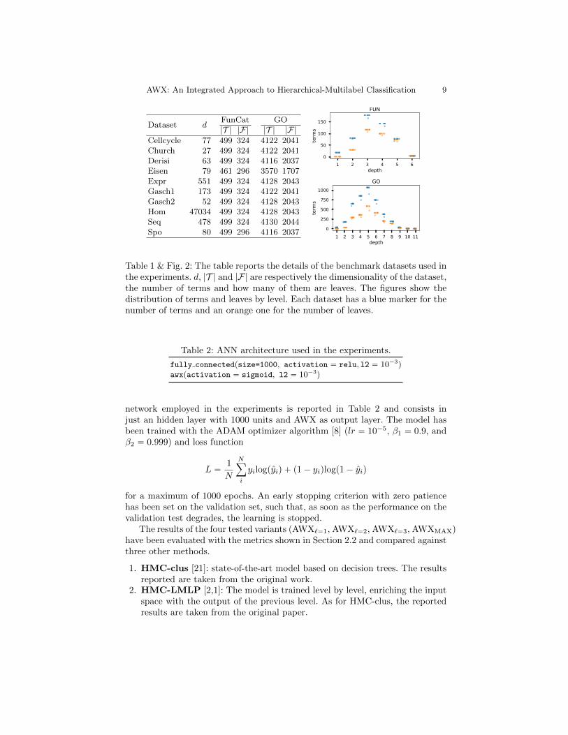
Table 1 & Fig. 2: The table reports the details of the benchmark datasets used inthe experiments. d, |T | and |F | are respectively the dimensionality of the dataset,the number of terms and how many of them are leaves. The figures show thedistribution of terms and leaves by level. Each dataset has a blue marker for thenumber of terms and an orange one for the number of leaves.

Table 2: ANN architecture used in the experiments.

fully connectedpsize=1000, activation “ relu, l2 “ 10´3q

awxpactivation “ sigmoid, l2 “ 10´3q

network employed in the experiments is reported in Table 2 and consists injust an hidden layer with 1000 units and AWX as output layer. The model hasbeen trained with the ADAM optimizer algorithm [8] (lr “ 10´5, β1 “ 0.9, andβ2 “ 0.999) and loss function

L “1

N

Nÿ

i

yilogpyiq ` p1´ yiqlogp1´ yiq

for a maximum of 1000 epochs. An early stopping criterion with zero patiencehas been set on the validation set, such that, as soon as the performance on thevalidation test degrades, the learning is stopped.

The results of the four tested variants (AWX`“1, AWX`“2, AWX`“3, AWXMAX)have been evaluated with the metrics shown in Section 2.2 and compared againstthree other methods.

1. HMC-clus [21]: state-of-the-art model based on decision trees. The resultsreported are taken from the original work.

2. HMC-LMLP [2,1]: The model is trained level by level, enriching the inputspace with the output of the previous level. As for HMC-clus, the reportedresults are taken from the original paper.


Table 3: AUCpPRq. Bold values show the best preforming method on the dataset.The standard deviation of the computed methods is in the range r0.001, 0.005sand r0.002, 0.008s respectively for FunCat and GO, with the only exception ofHom, where is an order of magnitude bigger.

CLUS-HMC HMC-LMLP MLPleaves AWX`“1 AWX`“2 AWX`“3 AWXMAX

FunCat

Cellcycle 0.172 0.185 0.148* 0.205* 0.189* 0.181* 0.174Church 0.170 0.164 0.102* 0.173 0.150* 0.136* 0.127*Derisi 0.175 0.170 0.112* 0.175 0.152* 0.142* 0.136*Eisen 0.204 0.208 0.196* 0.252* 0.243* 0.234* 0.225*Expr 0.210 0.196 0.201 0.262* 0.236* 0.229* 0.223*Gasch1 0.205 0.196 0.182 0.238* 0.227* 0.217* 0.209Gasch2 0.195 0.184 0.150* 0.211* 0.195 0.186 0.178*Hom 0.254 0.192 0.100* 0.107* 0.109* 0.106* 0.127*Seq 0.211 0.195 0.188* 0.253* 0.234* 0.227* 0.218Spo 0.186 0.172 0.117* 0.179 0.159* 0.150* 0.143*

GO

Cellcycle 0.357 0.365 0.315* 0.441* 0.406* 0.385* 0.362Church 0.348 0.347 0.272* 0.440* 0.378* 0.355* 0.329Derisi 0.355 0.349 0.274* 0.424* 0.376* 0.352 0.335*Eisen 0.380 0.403 0.347* 0.481* 0.449* 0.426* 0.410*Expr 0.368 0.384 0.357* 0.480* 0.437* 0.418* 0.407*Gasch1 0.371 0.384 0.346* 0.468* 0.437* 0.416* 0.401*Gasch2 0.365 0.369 0.328* 0.454* 0.417* 0.394* 0.379Hom 0.401 0.203* 0.264* 0.256* 0.242* 0.238*Seq 0.386 0.384 0.347* 0.472* 0.429* 0.412* 0.397*Spo 0.352 0.345 0.278* 0.420* 0.378* 0.355 0.336

3. MLPleaves : ANN trained only on the leaf terms with the same parametersof AWX. The prediction for the non-leaf terms are obtained by taking themax of the predictions for underlying terms in the hierarchy.

The comparison with MLPleaves is crucial, because it highlights the impact ofjointly learning the whole hierarchy with respect to inferring the prediction afterthe learning phase.

Both AWX and MLPleaves are based on ANNs, so, in order to mitigate theeffect of the random initialization of the weight matrix, the learning processhas been repeated 10 times. We report the average results of the 10 iterationsand the standard deviation ranges are reported in the caption of the tables. Weperformed a t-test with α “ 0.05 to assess the significativity of the differencewith respect to the state-of-the-art and marked with * the results that passedthe test.

No parameter tuning has been performed for the trained methods and thevalidation split has been used only for the early stopping criterion.

5 Results

In this section are reported and discussed the results obtained by the proposedmethod on ten benchmark datasets. Besides the comparison with the state-of-the-art, we will show the impact of AWX highlighting the differences with respectto MLPleaves.


Table 4: AUCPR. Bold values show the best preforming method on the dataset.HMC-LMLP provides no results for this metric, so it has been removed fromthe table. The standard deviation of the computed methods is in the ranger0.001, 0.005s for both FunCat and GO, with the only exception of Hom, whereit is an order of magnitude bigger.

CLUS-HMC MLPleaves AWX`“1 AWX`“2 AWX`“3 AWXMAX

FunCat

Cellcycle 0.034 0.068* 0.075* 0.076* 0.077* 0.076*Church 0.029 0.040* 0.040* 0.041* 0.040* 0.041*Derisi 0.033 0.047* 0.047* 0.048* 0.049* 0.048*Eisen 0.052 0.095* 0.103* 0.104* 0.106* 0.106*Expr 0.052 0.114* 0.120* 0.121* 0.121* 0.120*Gasch1 0.049 0.101* 0.108* 0.110* 0.111* 0.109*Gasch2 0.039 0.069* 0.080* 0.078* 0.077* 0.078*Hom 0.089 0.116 0.095 0.086 0.112 0.164Seq 0.053 0.126* 0.121* 0.126* 0.126* 0.124*Spo 0.035 0.043* 0.045* 0.045* 0.045* 0.045*

GO

Cellcycle 0.021 0.057* 0.059* 0.057* 0.057* 0.057*Church 0.018 0.034* 0.030* 0.032* 0.031* 0.031*Derisi 0.019 0.038* 0.041* 0.040* 0.040* 0.039*Eisen 0.036 0.082* 0.091* 0.089* 0.088* 0.088*Expr 0.029 0.092* 0.104* 0.102* 0.104* 0.102*Gasch1 0.030 0.076* 0.086* 0.086* 0.086* 0.085*Gasch2 0.024 0.065* 0.067* 0.066* 0.067* 0.066*Hom 0.051 0.071 0.042 0.046 0.042 0.053Seq 0.036 0.130* 0.130* 0.130* 0.128* 0.128*Spo 0.026 0.037* 0.038* 0.039* 0.040* 0.038*

Table 3 reports the micro-averaged area under the precision recall curve(AUCpPRq). AWX`“1 has a clear edge over the competitors, in both the ontolo-gies. With the FunCat annotation, it is significantly better then CLUS-HMCsix out of ten times and worse just in the Hom dataset, while with GO it winsnine out of ten times. AWX`“1 clearly outperforms also the other AWX versionsand MLPleaves in all the datasets. We can notice that the performance tends todecrease for higher values of `, and reaches the minimum with AWXMAX. Thiscan be explained by the distribution of the example-annotation: due to the TPR,the terms placed close to the root are more likely to be associated with moreexamples then the lower terms. With ` “ 1 each leaf, among the descendants,contributes equally to the prediction, boosting the prediction values of the upperterms.

Of great interest is the comparison between MLPleaves and AWXMAX. Wecan notice that AWXMAX, despite being the worst performing version of AWX,always outperforms MLPleaves. Remember that the main difference between thetwo architectures is that with AWXMAX prediction are propagated at learningtime and consequently optimized, while in MLPleaves the predictions of the non-leaf terms are inferred offline.

Table 4 reports the macro-averaged area under the precision recall curves(AUCPR). Unfortunately HMC-LMLP does not provide the score for this metric,but AWX clearly outperforms CLUS-HMC, both with the FunCat and with theGO annotations. We can notice that the differences are significant in all the


Table 5: AUCPRw. Bold values show the best preforming method on the dataset.HMC-LMLP provides no data for the GO datasets. The standard deviation ofthe computed methods is in the range r0.001, 0.005s for both FunCat and GO,with the only exception of Hom, where it is an order of magnitude bigger.

CLUS-HMC HMC-LMLP MLPleaves AWX`“1 AWX`“2 AWX`“3 AWXMAX

FunCat

Cellcycle 0.142 0.145 0.186* 0.200* 0.204* 0.205* 0.203*Church 0.129 0.118 0.132 0.139* 0.139* 0.139* 0.138Derisi 0.137 0.127 0.144* 0.150* 0.152* 0.152* 0.151*Eisen 0.183 0.163 0.229* 0.246* 0.254* 0.254* 0.252*Expr 0.179 0.167 0.239* 0.260* 0.260* 0.258* 0.255*Gasch1 0.176 0.157 0.217* 0.234* 0.241* 0.240* 0.237*Gasch2 0.156 0.142 0.183* 0.200* 0.202* 0.202* 0.200 *Hom 0.240 0.159 0.185 0.185 0.188 0.193 0.222Seq 0.183 0.112 0.232* 0.260* 0.263* 0.262* 0.258*Spo 0.153 0.129 0.152 0.159 0.161* 0.161* 0.160*

GO

Cellcycle 0.335 0.372* 0.379* 0.384* 0.385* 0.380*Church 0.316 0.325* 0.328* 0.331* 0.329* 0.327*Derisi 0.321 0.331* 0.334* 0.338* 0.337* 0.336*Eisen 0.362 0.402* 0.418* 0.426* 0.423* 0.418*Expr 0.353 0.407* 0.424* 0.430* 0.430* 0.427*Gasch1 0.353 0.397* 0.410* 0.421* 0.419* 0.416*Gasch2 0.347 0.379* 0.386* 0.394* 0.393* 0.388*Hom 0.389 0.354* 0.342* 0.349 0.345* 0.356Seq 0.373 0.408* 0.431* 0.436* 0.434* 0.430*Spo 0.324 0.333* 0.332 0.339* 0.339* 0.338*

datasets, with the exception of Hom, where the variance of the computed resultsis above 0.04 with FunCat and 0.007 with GO. Within AWX is instead moredifficult to identify a version that performs clearly better then the others, theirperformance are almost indistinguishable. Focusing on the differences betweenMLPleaves and AWXMAX, we can see that the former is outperformed fourteenout of twenty times by the latter. The advantage of the AWX layer in this caseis not as visible as in terms of AUCpPRq, because AUCPR gives equal weightto the curve for each class, ignoring the number of annotated examples. Withinour setting, where most of the classes have few examples, this evaluation metrictends to flatten the results, and may not be a good indicator of the performance.

Table 5 reports the weighted-average of the area under the precision recallcurves (AUCPRw). AWX has solid performance also considering this evaluationmetric, outperforming significantly CLUS-HMC in most of the datasets. HMC-LMLP provides results only for the FunCat-annotated datasets, but appears tobe not competitive with our method. Within the proposed variants of AWX,` “ 2 has an edge over ` “ 1 and MAX, while is almost indistinguishable from` “ 3. Moreover, comparing AWXMAX and MLPleaves, we can see that theformer is systematically better then the latter.

The results reported for AWX (in all its variants) and MLP were not ob-tained tuning the parameters on the validation sets, but rather setting them apriori. The lack of parameter-tuning is clear on the Hom dataset. With all theconsidered evaluation metrics, this dataset significantly diverges with respectto the others. This behaviour is common also to CLUS-HMC, but unlikely the


proposed methods, it has the best performance on this dataset. An explanationof this anomaly can be found in Table 1, where we can see the difference in thedimensionality. Hom dataset features are indeed two order of magnitude morethen the second biggest dataset, i.e. Expr. The sub-optimal choice of the modelparameters and the dimensionality could therefore explain the deviation of thisdataset from the performance trend, and these aspects should be explored in thefuture.

AWX has solid overall performance. AUCpPRq is the most challenging eval-uation metric, where the improvement over the state-of-the-art is smaller, whilewith the last two metrics, AWX appears to have a clear advantage. The choiceof the value for ` depends on the metric we want to optimize, indeed AWX per-forms the best with ` “ 1 considering AUCpPRq, while if we consider AUCPRqor AUCPRw values of ` “ 2 or ` “ 3 have an edge over the others. The directcomparison between MLPleaves and AWXMAX is clearly in favour of the latter,which wins almost on all the datasets. This highlights the clear impact of theproposed approach, that allows a jointly optimization of all the classes in thedatasets.

6 Conclusion

In this work we have proposed a generalization to the continuous domain of thetrue path rule and presented a novel ANN layer, named AWX. The aim of thiscomponent is to allow the user to compute consistent hierarchical predictions ontop of any deep learning architecture. Despite the simplicity of the proposed ap-proach, it appears clear that AWX has an edge over the state-of-the-art methodCLUS-HMC. Significant improvements can be seen almost on all the datasetsfor the macro and weighted averaged area under the precision recall curves eval-uation metric, while the advantage in terms of AUCpPRq is significant in six outof ten datasets.

Part of improvement could be attributed to the power and flexibility of ANNover decision trees, but we have shown that AWX systematically outperformsalso HMC-LMLP, based on ANN, and MLPleaves, that has exactly the samearchitecture as AWX, but with sigmoid output layer just for the leaf terms.

Further work will be focused to test the proposed methods with real-worldchallenging datasets, integrating AWX in deep learning architectures. Anotherinteresting aspect will be to investigate the performance of AWX with semantic-based metrics, both globally or considering only the leaf terms.

References

1. Ricardo Cerri, Rodrigo C. Barros, and Andre C. P. L. F. de Carvalho. Hierarchicalclassification of Gene Ontology-based protein functions with neural networks. 2015Int. Jt. Conf. Neural Networks, pages 1–8, 2015.

2. Ricardo Cerri, Rodrigo C. Barros, and Andre C.P.L.F. de Carvalho. Hierarchi-cal multi-label classification using local neural networks. J. Comput. Syst. Sci.,80(1):39–56, 2014.


3. Francois Chollet et al. Keras, 2015.

4. Gene Ontology Consortium. Creating the gene ontology resource: design and im-plementation. Genome Res., 11(8):1425–33, 2001.

5. Qingtian Gong, Wei Ning, and Weidong Tian. GoFDR: A Sequence AlignmentBased Method for Predicting Protein Functions. Methods, 93:3–14, 2015.

6. Geoffrey Hinton, Li Deng, Dong Yu, George E Dahl, Abdel-rahman Mohamed,Navdeep Jaitly, Andrew Senior, Vincent Vanhoucke, Patrick Nguyen, Tara NSainath, et al. Deep neural networks for acoustic modeling in speech recogni-tion: The shared views of four research groups. IEEE Signal Processing Magazine,29(6):82–97, 2012.

7. Yuxiang Jiang et al. An expanded evaluation of protein function prediction meth-ods shows an improvement in accuracy. Genome biology, pages 1–17, 2016.

8. Diederik Kingma and Jimmy Ba. Adam: A method for stochastic optimization.arXiv preprint arXiv:1412.6980, 2014.

9. Alex Krizhevsky, Ilya Sutskever, and Geoffrey E Hinton. Imagenet classificationwith deep convolutional neural networks. In Advances in neural information pro-cessing systems, pages 1097–1105, 2012.

10. Alexey G Murzin, Steven E Brenner, Tim Hubbard, and Cyrus Chothia. Scop: astructural classification of proteins database for the investigation of sequences andstructures. Journal of molecular biology, 247(4):536–540, 1995.

11. Guillaume Obozinski, Gert Lanckriet, Charles Grant, Michael I Jordan, andWilliam Stafford Noble. Consisten probabilistic outputs for protein function pre-diction. Genome biology, 9(65):1–19, 2008.

12. Predrag Radivojac, Wyatt T Clark, Tal Ronnen Oron, Alexandra M Schnoes,Tobias Wittkop, Artem Sokolov, Kiley Graim, Christopher Funk, Karin Verspoor,Asa Ben-Hur, Gaurav Pandey, and Jeffrey M Yunes. A large-scale evaluation ofcomputational protein function prediction. Nature Methods, 10(3):221–227, 2013.

13. Andreas Ruepp, Alfred Zollner, Dieter Maier, Kaj Albermann, Jean Hani, MartinMokrejs, Igor Tetko, Ulrich Guldener, Gertrud Mannhaupt, Martin Munsterkotter,and H. Werner Mewes. The FunCat, a functional annotation scheme for systematicclassification of proteins from whole genomes. Nucleic Acids Research, 32(18):5539–5545, 2004.

14. Lynn Marie Schriml, Cesar Arze, Suvarna Nadendla, Yu-Wei Wayne Chang, MarkMazaitis, Victor Felix, Gang Feng, and Warren Alden Kibbe. Disease ontology: abackbone for disease semantic integration. Nucleic acids research, 40(D1):D940–D946, 2011.

15. Artem Sokolov and Asa Ben-Hur. Hierarchical classification of gene ontology termsusing the gostruct method. Journal of bioinformatics and computational biology,8(02):357–376, 2010.

16. Radu Soricut and Daniel Marcu. Sentence level discourse parsing using syntacticand lexical information. In Proceedings of the 2003 Conference of the North Ameri-can Chapter of the Association for Computational Linguistics on Human LanguageTechnology-Volume 1, pages 149–156. Association for Computational Linguistics,2003.

17. Mohammad S Sorower. A literature survey on algorithms for multi-label learning.Oregon State University, Corvallis, 18, 2010.

18. Nitish Srivastava, Geoffrey Hinton, Alex Krizhevsky, Ilya Sutskever, and RuslanSalakhutdinov. Dropout: A simple way to prevent neural networks from overfitting.The Journal of Machine Learning Research, 15(1):1929–1958, 2014.


19. Aixin Sun and Ee-Peng Lim. Hierarchical text classification and evaluation. InData Mining, 2001. ICDM 2001, Proceedings IEEE International Conference on,pages 521–528. IEEE, 2001.

20. Isaac Triguero and Celine Vens. Labelling strategies for hierarchical multi-labelclassification techniques. Pattern Recognit., pages 1–14, 2015.

21. Celine Vens, Jan Struyf, Leander Schietgat, Saso Dzeroski, and Hendrik Blockeel.Decision trees for hierarchical multi-label classification. Mach. Learn., 73(2):185–214, 2008.

22. Min Ling Zhang and Zhi Hua Zhou. A review on multi-label learning algorithms.IEEE Trans. Knowl. Data Eng., 26(8):1819–1837, 2014.

awx: an integrated approach to hierarchical-multilabel ... · awx: an integrated approach to...

Documents