Axion Cosmology

David J. E. Marsh1

1 Department of Physics,King’s College London,

Strand, London, WC2R 2LS,United Kingdom.

Abstract

Axions comprise a broad class of particles that can play a major role in explainingthe unknown aspects of cosmology. They are also well-motivated within high energyphysics, appearing in theories related to CP -violation in the standard model, super-symmetric theories, and theories with extra-dimensions, including string theory, andso axion cosmology offers us a unique view onto these theories. I review the motivationand models for axions in particle physics and string theory. I then present a compre-hensive and pedagogical view on the cosmology and astrophysics of axion-like particles,starting from inflation and progressing via BBN, the CMB, reionization and structureformation, up to the present-day Universe. Topics covered include: axion dark matter(DM); direct and indirect detection of axions, reviewing existing and future experi-ments; axions as dark radiation; axions and the cosmological constant problem; decaysof heavy axions; axions and stellar astrophysics; black hole superradiance; axions andastrophysical magnetic fields; axion inflation, and axion DM as an indirect probe ofinflation. A major focus is on the population of ultralight axions created via vacuumrealignment, and its role as a DM candidate with distinctive phenomenology. Cosmo-logical observations place robust constraints on the axion mass and relic density inthis scenario, and I review where such constraints come from. I next cover aspectsof galaxy formation with axion DM, and ways this can be used to further search forevidence of axions. An absolute lower bound on DM particle mass is established. Itis ma > 10−24 eV from linear observables, extending to ma & 10−22 eV from non-linear observables, and has the potential to reach ma & 10−18 eV in the future. Thesebounds are weaker if the axion is not all of the DM, giving rise to limits on the relicdensity at low mass. This leads to the exciting possibility that the effects of axionDM on structure formation could one day be detected, and the axion mass and relicdensity measured from cosmological observables.

KCL-PH-TH/2015-50

arX

iv:1

510.

0763

3v2

[as

tro-

ph.C

O]

15

Jun

2016

Contents

1 Introduction 3

2 Models 62.1 The QCD Axion . . . . . . . . . . . . . . . . . . . . . . . . . . . . . . . . . 6

2.1.1 The Strong-CP Problem and the PQ Solution . . . . . . . . . . . . 62.1.2 PQWW axion . . . . . . . . . . . . . . . . . . . . . . . . . . . . . . . 72.1.3 KSVZ axion . . . . . . . . . . . . . . . . . . . . . . . . . . . . . . . . 82.1.4 DFSZ axion . . . . . . . . . . . . . . . . . . . . . . . . . . . . . . . . 9

2.2 Anomalies, Instantons, and the Axion Potential . . . . . . . . . . . . . . . . 102.3 Couplings to the Standard Model . . . . . . . . . . . . . . . . . . . . . . . . 122.4 Axions in String Theory . . . . . . . . . . . . . . . . . . . . . . . . . . . . . 13

3 Production and Initial Conditions 173.1 Symmetry Breaking and Non-Perturbative Physics . . . . . . . . . . . . . . 173.2 The Axion Field During Inflation . . . . . . . . . . . . . . . . . . . . . . . . 18

3.2.1 PQ symmetry unbroken during inflation, fa < HI/2π . . . . . . . . 193.2.2 PQ symmetry broken during inflation, fa > HI/2π . . . . . . . . . . 20

3.3 Cosmological Populations of Axions . . . . . . . . . . . . . . . . . . . . . . 203.3.1 Decay Product of Parent Particle . . . . . . . . . . . . . . . . . . . . 213.3.2 Decay Product of Topological Defect . . . . . . . . . . . . . . . . . . 223.3.3 Thermal Production . . . . . . . . . . . . . . . . . . . . . . . . . . . 233.3.4 Vacuum Realignment . . . . . . . . . . . . . . . . . . . . . . . . . . 24

4 The Cosmological Axion Field 244.1 Action and Energy Momentum Tensor . . . . . . . . . . . . . . . . . . . . . 254.2 Background Evolution . . . . . . . . . . . . . . . . . . . . . . . . . . . . . . 254.3 Misalignment Production of DM Axions . . . . . . . . . . . . . . . . . . . . 26

4.3.1 Axion-Like Particles . . . . . . . . . . . . . . . . . . . . . . . . . . . 264.3.2 The QCD Axion . . . . . . . . . . . . . . . . . . . . . . . . . . . . . 30

4.4 Cosmological Perturbation Theory . . . . . . . . . . . . . . . . . . . . . . . 334.4.1 Initial Conditions . . . . . . . . . . . . . . . . . . . . . . . . . . . . . 344.4.2 Early Time Treatment . . . . . . . . . . . . . . . . . . . . . . . . . . 354.4.3 The Axion Effective Sound Speed . . . . . . . . . . . . . . . . . . . . 364.4.4 Growth of Perturbations and the Axion Jeans Scale . . . . . . . . . 364.4.5 Transfer Functions: Relation to WDM and Neutrinos . . . . . . . . 39

4.5 Non-linearities and the Schrodinger Picture . . . . . . . . . . . . . . . . . . 414.6 Simulating axion DM . . . . . . . . . . . . . . . . . . . . . . . . . . . . . . . 434.7 My Two Cents on BEC . . . . . . . . . . . . . . . . . . . . . . . . . . . . . 44

5 Constraints from the CMB and LSS 475.1 The Primary CMB . . . . . . . . . . . . . . . . . . . . . . . . . . . . . . . . 475.2 The Matter Power Spectrum . . . . . . . . . . . . . . . . . . . . . . . . . . 485.3 Combined Constraints . . . . . . . . . . . . . . . . . . . . . . . . . . . . . . 505.4 Isocurvature and Axions as a Probe of Inflation . . . . . . . . . . . . . . . . 52

6 Galaxy Formation 556.1 The Halo Mass Function . . . . . . . . . . . . . . . . . . . . . . . . . . . . . 556.2 Constraints from High-z and the EOR . . . . . . . . . . . . . . . . . . . . . 576.3 Halo Density Profiles . . . . . . . . . . . . . . . . . . . . . . . . . . . . . . . 596.4 ULAs and the CDM Small Scale Crises . . . . . . . . . . . . . . . . . . . . 61

1

7 Axions and Accelerated Expansion 657.1 Axions and the Cosmological Constant Problem . . . . . . . . . . . . . . . . 657.2 Axion Inflation . . . . . . . . . . . . . . . . . . . . . . . . . . . . . . . . . . 67

7.2.1 Natural Inflation and Variants . . . . . . . . . . . . . . . . . . . . . 687.2.2 Axion Monodromy . . . . . . . . . . . . . . . . . . . . . . . . . . . . 70

8 Gravitational Interactions with Black Holes and Pulsars 718.1 Black Hole Superradiance . . . . . . . . . . . . . . . . . . . . . . . . . . . . 718.2 Pressure Oscillations and Pulsar Timing . . . . . . . . . . . . . . . . . . . . 72

9 Non-Gravitational Interactions 739.1 Stellar Astrophysics . . . . . . . . . . . . . . . . . . . . . . . . . . . . . . . 749.2 “Light Shining Through a Wall” . . . . . . . . . . . . . . . . . . . . . . . . 769.3 Vacuum Birefringence and Dichroism . . . . . . . . . . . . . . . . . . . . . . 769.4 Axion Mediated Forces . . . . . . . . . . . . . . . . . . . . . . . . . . . . . . 779.5 Direct Detection of Axion DM . . . . . . . . . . . . . . . . . . . . . . . . . 77

9.5.1 Haloscopes and ADMX . . . . . . . . . . . . . . . . . . . . . . . . . 779.5.2 Nuclear Magnetic Resonance and CASPEr . . . . . . . . . . . . . . 78

9.6 Heavy Axions and Axion Decays . . . . . . . . . . . . . . . . . . . . . . . . 809.7 Axion Dark Radiation . . . . . . . . . . . . . . . . . . . . . . . . . . . . . . 819.8 Axions and Astrophysical Magnetic Fields . . . . . . . . . . . . . . . . . . . 83

9.8.1 CMB Spectral Distortions . . . . . . . . . . . . . . . . . . . . . . . . 839.8.2 X-ray Production . . . . . . . . . . . . . . . . . . . . . . . . . . . . . 84

9.9 Cosmological Birefringence . . . . . . . . . . . . . . . . . . . . . . . . . . . 84

10 Concluding Remarks 86

A Theta Vacua of Gauge Theories 87

B EFT for Cosmologists 89

C Friedmann Equations 90

D Cosmological Fluids 91

E Bayes Theorem and Priors 92

F Degeneracies and Sampling with ULAs 93

G Sheth-Tormen Halo Mass Function 95

2

1 Introduction

As Weinberg said, “physics thrives on crisis” [1]. In 1989 when Weinberg wrote that famousreview, he said that physics was short on crises. Happily, these days, thanks in large partto the advent of precision cosmology, it is full of them.

The standard cosmological model is described by just six numbers: two for initial condi-tions, one for dark matter (DM), one for the baryons, one for cosmic structure formation andreionization, and one for the cosmological constant (c.c.). Each of these numbers presents aproblem for our understanding of fundamental physics. The initial conditions appear closeto scale invariant: producing such initial conditions requires a period of rapid acceleration(or slow deceleration) in the early Universe, a state of affairs that cannot be realised in theusual hot big bang. Dark matter constitutes the vast majority of matter in the Universe,and no particle in the standard model of particle physics can fit the role of being stable,cold, and weakly coupled. The standard model also provides no obvious way to tip thematter-anti-matter asymmetry in favour of baryons instead of anti-baryons. Structure for-mation and reionization are sensitive to the initial conditions, matter content, and complexastrophysical processes in ways that we are only just learning. And then finally there isWeinberg’s problem of the c.c..

In 1989 Weinberg selected just the c.c. as a major problem: even without precisioncosmology, it was clear that the theoretical expectations about this number were wildly offthe mark. All of the other problems were known at that time, but without the precisionmeasurements we have today their importance could easily be debated and there was noneed to call “crisis.” We are no longer in that position of blissful ignorance: all the numbersin the standard cosmological model need to be considered and their theoretical implicationstaken seriously.

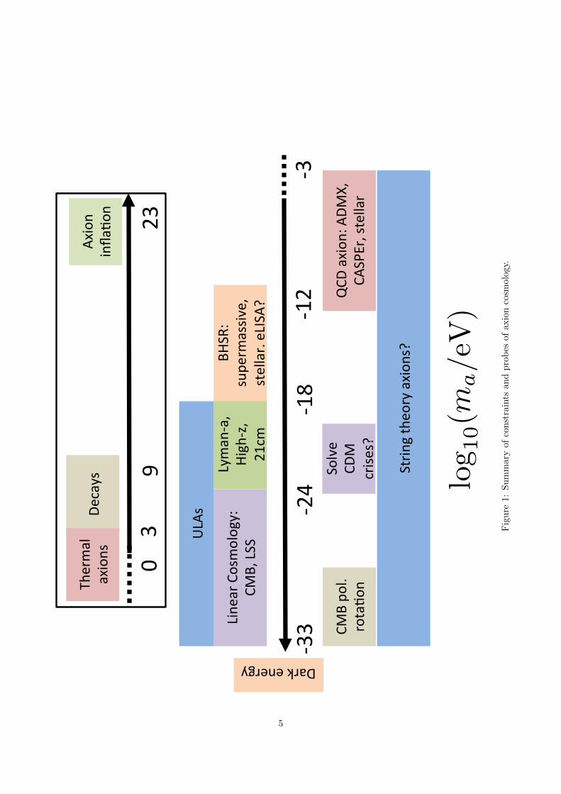
In seeking a unified view of the problems presented by precision cosmology, we will focusin this review on a class of particles known as axions. Ever since the earliest days of theQCD axion it has been realised that it offers an exceptionally good DM candidate. Withthe advent of string theory and the corresponding profusion of axion-like particles (ALPs),axions have come to play important roles in inflation and the generation of cosmologicalinitial conditions, and in the solution of the c.c. problem. String axions also offer theposisbility to resolve problems of structure formation inherent in more vanilla models ofDM. Axions can even assist in baryogenesis thanks to their role in CP -violation. A summaryof constraints and probes of axion cosmology, as a function of axion mass, is shown in Fig. 1.

A large portion of this review will focus on ALPs in the mass range

10−33 eV . ma . 10−18 eV . (1)

I will refer to axions in this mass range as ultralight axions, or ULAs. The lower bound is oforder the present day Hubble constant, H0/h = MH = 2.13×10−33 eV = 100 km s−1 Mpc−1,and reflects constraints on axion dark energy (DE). The upper bound is related to the baryonJeans scale, and reflects a distinctive role of ULAs in cosmological structure formation andreionization. This vast range of axion masses can be probed using the tools that led usto our crises in the first place, i.e. those of precision cosmology: the cosmic microwavebackground (CMB), large scale structure (LSS), galaxy formation in the local Universe andat high redshift, and by the epoch of reionization (EOR).

It is worth noting here, for clarity, that the word “axion” can take on a variety ofmeanings. It was first coined by Wilczek [2] to name the particle associated to the axialanomaly in QCD and the Peccei-Quinn [3] solution to the strong-CP problem. It is sonamed after the eponymous American laundry detergent, using the axial anomaly to cleanup the mess of CP symmetry in the strong interactions [4]. The QCD axion acquiresmass from QCD chiral symmetry breaking, giving a one parameter model described by theaxion decay constant, fa. In quantum field theory, the term can apply generally to anypseudoscalar Goldstone bosons of spontaneously broken global chiral symmetries, typically

3

giving a two parameter model with (ma, fa). In string theory and supergravity, the term“axion” is more general and can refer either to such matter fields, or to pseudoscalar fieldsassociated to the geometry of compact spatial dimensions [5]. In these theories there aretypically many axion fields, each with a number of free parameters in their potentialsand kinetic terms. In this review, we will use the term in its most general sense for a lightpseudoscalar field (indeed in some cosmological cases, apart from naturalness considerations,even the distinction between scalar and pseudoscalar will be irrelevant).

Since the QCD axion was first proposed in 1977-1978, there have been many reviewswritten on axion physics. Many such reviews and published lecture notes focus on the QCDaxion and its role in solving the strong-CP problem [6, 7], as well as its important cosmo-logical role [8]. Of ALPs, there are technical reviews of axions in field theory and stringtheory [9, 5], as well as reviews of axions in astrophysics [10], and of axion inflation [11].There is also a vast number of reviews in the field of axion direct detection [12, 13, 14, 15, 16].It is the purpose of this review firstly to focus on ULAs, the cosmology of which has notbeen reviewed before, and with a particular emphasis on methods of modern precision cos-mology, including computational aspects both analytic and numerical, and with an eye todata. Secondly, it is to bring together the disparate topics of other axion reviews into oneplace, expressing the unity of axion particle physics and cosmology: a task, which, to myknowledge, has not been fully addressed since the review of Ref. [9], more than 30 yearsago in this very journal.

Notes

Useful notation and equations for cosmology are defined in the Appendix. I (mostly) useunits where c = ~ = kB = 1 and express everything in terms of either electronvolts, eV, solarmasses, M, parsecs, pc, or Kelvin, K, depending on the context. The Fourier conjugatevariable to x is k and my Fourier convention puts the 2π’s under the dk’s. I use the reducedPlanck mass, Mpl = 1/

√8πG = 2.435× 1027 eV, and a “mostly positive” metric signature.

4

log10(m

a/eV

)

3"23"

9"

Decays"

Axion

"infla1on

"

0"

Thermal"

axions"

818"

83"

833"

812"

824"

Line

ar"Cosmology:"

CMB,"LSS"

Lyman8a,"

High8z,"

21cm

"

QCD

"axion

:"ADMX,"

CASPEr,"stellar"

String"the

ory"axions?"

BHSR:"

supe

rmassive,"

stellar."eLISA

?"

CMB"po

l."rota1on

""

Solve"

CDM"

crises?"

ULAs"

Dark"energy"

Fig

ure

1:S

um

mary

of

con

stra

ints

an

dp

rob

esof

axio

nco

smolo

gy.

5

2 Models

A classic review of models for axions in particle physics and string theory is Ref. [9], wheremany more details are given. A modern review of axions in string theory is Ref. [5], andfor pedagogical introductions and phenomenology see e.g. Refs. [17, 14]. This section isintended only as an overview: we will wave our hands through the particle physics com-putations, and wave them even more wildly through the string theory. This section is alsoself-contained, and can be skipped for those interested only in cosmology and astrophysics.The salient points for cosmology are repeated in Section 3.1.

2.1 The QCD Axion

2.1.1 The Strong-CP Problem and the PQ Solution

QCD suffers from the “strong-CP problem.” A topological (total derivative) term is allowedin the Lagrangian:

LθQCD =θQCD

32π2Tr GµνG

µν , (2)

where Gµν is the gluon field strength tensor, Gµν = εµναβGαβ/2 is its dual, and the traceis over the adjoint representation of SU(3) (a notation I drop from now on).1 This termarises due to the so-called “θ-vacua” of QCD [18], which are discussed in Appendix A.

The θ term is CP violating and gives rise to an electric dipole moment (EDM) for theneutron [19]:

dn ≈ 3.6× 10−16θQCD e cm , (3)

where e is the charge on the electron. The (permanent, static) dipole moment is constrainedto |dn| < 2.9× 10−26 e cm (90% C.L.) [20], implying θQCD . 10−10.

This is a true fine tuning problem, since θQCD could obtain an O(1) contribution fromthe observed CP -violation in the electroweak (EW) sector [21], which must be cancelled tohigh precision by the (unrelated) gluon term. Specifically, the measurable quantity is

θQCD = θQCD + arg detMuMd , (4)

where θ is the bare quantity and Mu, Md are the quark mass matrices.2

The QCD axion is the dynamical pseudoscalar field coupling to GG, proposed by Pecceiand Quinnn (PQ) [3], which dynamically sets θQCD = 0 via QCD non-perturbative effects(instantons) [23]. The simple idea is that there is a field, φ, which enjoys a shift symmetry,with only derivatives of φ appearing in the action. Taking θQCD = Cφ/fa, where φ is thecanonically normalized axion field, fa is the axion decay constant and C is the “colouranomaly” (discussed in Section 2.2), this is a symmetry under φ → φ + const. Then, aslong as shift symmetry violation is induced only by quantum effects as (Cφ/fa)GG, anycontribution to θQCD can be absorbed in a shift of φ. The action, and thus the potential

induced by QCD non-perturbative effects, only depends on the overall field multiplying GG.If the potential for the shifted field is minimized at Cφ/fa = 0 mod 2π, then the strong CPproblem is solved. In fact, a theorem of Vafa and Witten [23] guarantees that the instantonpotential is minimized at the CP conserving value. We will discuss the instanton potentialin more detail in Section 2.2.

1I have chosen the normalization for the gluon field, Aµ, appropriate for the vacuum topological term,which takes θQCD ∈ [0, 2π]. In this normalization the gluon kinetic term is −GµνGµν/4g2

3 , where g3 is theSU(3) gauge coupling constant.

2The phase of the quark mass matrix is not measured, but could be O(1). CP -violation in the standardmodel leads to a calculable minimum value for θQCD even in the axion model (e.g. Ref. [22]).

6

The axion mass, ma, induced by QCD instantons can be calculated in chiral perturbationtheory [24, 2]. It is given by

ma,QCD ≈ 6× 10−6 eV

(1012 GeV

fa/C

). (5)

This is a (largely) model-independent statement, and the approximate symbol, “≈,” takesmodel and QCD uncertainties into account. If fa is large, the QCD axion can be extremelylight and stable, and is thus an excellent DM candidate [25, 26, 27].

We will consider three general types of QCD axion model:3

• The Peccei-Quinn-Weinberg-Wilczek (PQWW) [3, 24, 2] axion, which introduces oneadditional complex scalar field only, tied to the EW Higgs sector. It is excluded byexperiment.

• The Kim-Shifman-Vainshtein-Zakharov (KSVZ) [28, 29] axion, which introduces heavyquarks as well as the PQ scalar.

• The Dine-Fischler-Srednicki-Zhitnitsky (DFSZ) [30, 31] axion, which introduces anadditional Higgs field as well as the PQ scalar.

2.1.2 PQWW axion

The PQWW model introduces a single additional complex scalar field, ϕ, to the standardmodel as a second Higgs doublet. One Higgs field gives mass to the u-type quarks, whilethe other gives mass to the d-type quarks (a freedom of the model is the choice of whichdoublet, if not a third field, gives mass to the leptons). This fixes the representation ofϕ in SU(2) × U(1). The whole Lagrangian is then taken to be invariant under a globalU(1)PQ symmetry, which acts with chiral rotations, i.e. with a factor of γ5. These chiralrotations shift the angular part of ϕ by a constant. The PQ field couples to the standardmodel via the Yukawa interactions which give mass to the fermions as in the usual Higgsmodel. The invariance of these terms under global U(1)PQ rotations fixes the PQ chargesof the fermions.

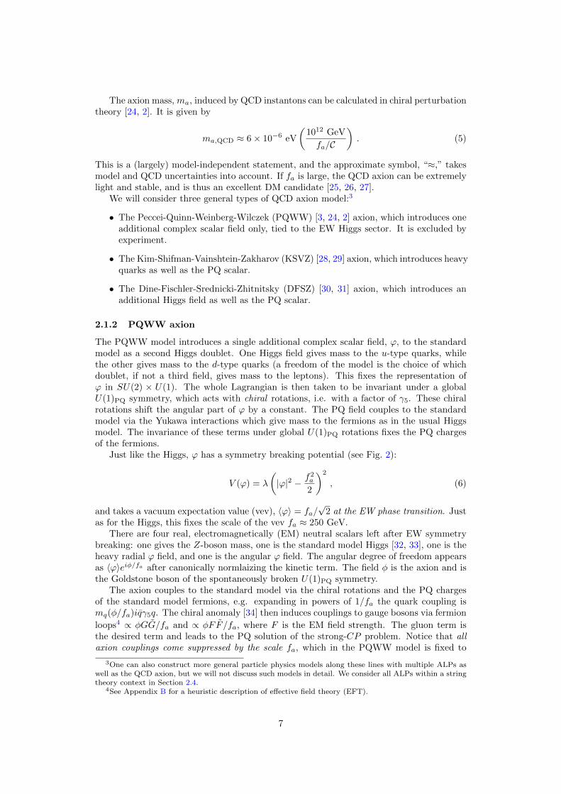
Just like the Higgs, ϕ has a symmetry breaking potential (see Fig. 2):

V (ϕ) = λ

(|ϕ|2 − f2

a

2

)2

, (6)

and takes a vacuum expectation value (vev), 〈ϕ〉 = fa/√

2 at the EW phase transition. Justas for the Higgs, this fixes the scale of the vev fa ≈ 250 GeV.

There are four real, electromagnetically (EM) neutral scalars left after EW symmetrybreaking: one gives the Z-boson mass, one is the standard model Higgs [32, 33], one is theheavy radial ϕ field, and one is the angular ϕ field. The angular degree of freedom appearsas 〈ϕ〉eiφ/fa after canonically normlaizing the kinetic term. The field φ is the axion and isthe Goldstone boson of the spontaneously broken U(1)PQ symmetry.

The axion couples to the standard model via the chiral rotations and the PQ chargesof the standard model fermions, e.g. expanding in powers of 1/fa the quark coupling ismq(φ/fa)iqγ5q. The chiral anomaly [34] then induces couplings to gauge bosons via fermion

loops4 ∝ φGG/fa and ∝ φFF/fa, where F is the EM field strength. The gluon term isthe desired term and leads to the PQ solution of the strong-CP problem. Notice that allaxion couplings come suppressed by the scale fa, which in the PQWW model is fixed to

3One can also construct more general particle physics models along these lines with multiple ALPs aswell as the QCD axion, but we will not discuss such models in detail. We consider all ALPs within a stringtheory context in Section 2.4.

4See Appendix B for a heuristic description of effective field theory (EFT).

7

Figure 2: A symmetry breaking potential in the complex ϕ plane. The vev of the radialmode is fa/

√2 and the axion is the massless angular degree of freedom at the potential

minimum.

be the EW vev. In the PQWW model fa is too small, the axion couplings are too large,and it is excluded, e.g. by beam-dump experiments [9]. The PQWW axion is also excludedby collider experiments such as LEP (see the recent compilation of collider constraints inRef. [35], and Section 9.6).

In the KSVZ and DFSZ models, which we now turn to, the PQ field, ϕ, is introducedindependently of the EW scale. The decay constant is thus a free parameter in these models,and can be made large enough such that they are not excluded. For this reason, both theKSVZ and the DFSZ axions are known as invisible axions. On the plus side, in these modelsthe axion is stable and is an excellent DM candidate with its own phenomenology.

2.1.3 KSVZ axion

The KSVZ axion model introduces a heavy quark doublet, QL, QR, each of which is anSU(3) triplet, and the subscripts represent the charge under chiral rotations. The PQscalar field, ϕ, has charge 2 under chiral rotations, but is now a standard model singlet.The PQ field and the heavy quarks interact via the PQ-invariant Yukawa term, whichprovides the heavy quark mass:

LY = −λQϕQLQR + h.c. , (7)

where the Yukawa coupling λQ is a free parameter of the model. As in the PQWW model,there is a global U(1)PQ symmetry which acts as a chiral rotation with angle α = φ/fa,shifting the axion field. Global U(1)PQ symmetry is spontaneously broken by the potential,Eq. 6.

At the classical level, the Lagrangian is unaffected by chiral rotations, and ϕ is notcoupled to the standard model. However at the quantum level, chiral rotations on Q affectthe GG term via the chiral anomaly [34]:

L → L+α

32π2GG , (8)

where I have used that in the KSVZ model the colour anomaly is equal to unity (seeSection 2.2).

8

At low energies, after PQ symmetry breaking, ϕ takes a vev and the Q fields obtaina large mass, mQ ∼ λQfa. The Q fields can then be integrated out. The chiral anomaly

induces the axion coupling to GG as a “memory” of the chiral rotation applied at highenergy. At the level of EFT, the induced topological term is the only modification to thestandard model Lagrangian: the KSVZ axion has no unsuppressed tree-level couplings tostandard model matter fields.

There is an axion-photon coupling in this model that can be calculated via loops givingthe EM anomaly. It’s value depends on the electromagnetic charges assigned to the Q fields.The canonical choice is that they are uncharged and the axion-photon coupling is inducedsolely by the longitudinal mode of the Z-boson (see e.g. Ref. [36]). Other couplings canalso be induced by loops and mixing, since Q must be charged under SU(3). Couplingswill be listed and discussed further in Section 2.3.

2.1.4 DFSZ axion

The DFSZ axion couples to the standard model via the Higgs sector. It contains two Higgsdoublets, Hu, Hd, like in the PQWW model, however the complex scalar, ϕ, which containsthe axion as its angular degree of freedom, is introduced as a standard model singlet. Again,global U(1)PQ symmetry is imposed and spontaneously broken by the potential, Eq. (6).

The PQ and Higgs fields interact via the scalar potential:

V = λHϕ2HuHd . (9)

This term is PQ invariant for ϕ with U(1)PQ charge +1, and the Higgs fields each withcharge -1. As in the KSVZ model, PQ rotations act by shifting the axion by φ/fa →φ/fa + α. When the PQ symmetry is broken and ϕ obtains a vev, the parameters in theHiggs potential, and the coupling constant, λH , must be chosen such that the Higgs fieldsremain light, consistent with the observed 125 GeV standard model Higgs [32, 33], and theEW vev, vEW =

√〈Hu〉2 + 〈Hd〉2.

The Higgs must also couple to all the standard model fermions, providing their massthrough Yukawa terms as usual, e.g.

LY ⊃ λuqLuRHu . (10)

In order for this to be PQ invariant the standard model fermions must be charged underU(1)PQ. After EW symmetry breaking, H is replaced by its vev, inducing axial currentcouplings between the axion and standard model fermions from the chiral term in thefermion mass matrix: mu(φ/fa)iuγ5u. This axial current in turn induces the couplingbetween the axion and GG via the colour anomaly. The difference between KSVZ andDFSZ is that for DFSZ this term is induced by light quark loops calculated at low energy,rather than via the integrating out of a heavy quark. In the DFSZ model all of the standardmodel quarks are charged under the PQ symmetry, giving rise to a larger colour anomaly,C = 6.

The same fermion loops induce the axion-photon coupling, φFF , which is computed viathe electromagnetic anomaly. Freedom in this model appears through the lepton charges:we are free to choose whether it is Hu or Hd that gives mass to the electron via Hu,d

¯LeR.

The axion-photon coupling is the sum of quark and lepton loops, and the different leptonPQ charges give different values for the anomaly, and thus the coupling (see Section 2.3).

The use of the Higgs in DFSZ leads to a number of important consequences that differ-entiate it from KSVZ. Firstly, in the DFSZ model there are tree-level couplings between theaxion and standard model fermions, via the chiral terms in the mass matrix. Secondly, theEW sector is modified by the addition of an extra axial Higgs field, A, with mass of order theEW scale. This is constrained by collider data, and could potentially be discovered at theLHC, just like the additional Higgs fields of supersymmetry (SUSY, see e.g. Refs. [37, 38]).

9

2.2 Anomalies, Instantons, and the Axion Potential

A PQ rotation on a field xi with PQ charge QPQ,i acts as

xi → eiQPQ,iφ/faxi . (11)

The rotation is chiral, meaning that, if xi is a spinor, left and right handed componentsof xi have opposite charges (for the two-component spinor ψ = (ψL, ψR) one introduces afactor of γ5 to achieve this).

The axion model is set up so that at the classical level the Lagrangian is invariant undersuch transformations, which leads to the shift symmetry of the axion field, φ→ φ+ const.At the quantum level, however, PQ rotations of quarks are anomalous, meaning that thequantum theory violates the classical symmetry. This affects the QCD topological term,and shifts it by an amount ∝ (φ/fa)GG. The question we now wish to answer is: what isthe constant of proportionality?

The constant of proportionality is called the colour anomaly of the PQ symmetry, andis given by (e.g. Ref. [39]):

Cδab = 2Tr QPQTaTb , (12)

where the trace is over all the fermions in the theory, and Ta are the generators of the SU(3)representations of the fermions (e.g. for the triplet these are the Gell-Mann matrices). APQ rotation now shows up in the action as

S → S +

∫d4x

C32π2

φ

faTrGµνG

µν . (13)

Although the topological term in the QCD action, Eq. (2), does not affect the classicalequations of motion, it does affect the vacuum structure, and the vacuum energy dependson θQCD. This is because of the existence of instantons and the so-called θ-vacua of QCD(for more details, see Ref. [18] and Appendix A). These emerge because the non-Abeliangauge group, SU(3), can be mapped onto the symmetry group of the space-time boundary,allowing for topologically-distinct field configurations [18]. The different vacua of QCD arelabelled by the value of θQCD. The vacuum energy is [40, 41]:

Evac ∝ cos θQCD ∼ θ2QCD . (14)

However, because the θ-vacua are topologically distinct, no process allows for transitionsbetween them, and the energy cannot be minimized.5 Introducing a field that couplesto GG, as the axion does, means that the vacuum energy now depends on the linearcombination Evac(θQCD + Cφ/fa).

Using the shift symmetry on φ to absorb any contribution to θQCD, the vacuum energyis

Evac ∝ cos

(Cφfa

). (15)

The vacuum energy now depends on a dynamical field, and so can be minimized by theequations of motion.

The colour anomaly sets the number of vacua that φ has in the range [0, 2πfa]. Becauseφ is an angular variable, we must have a symmetry under φ→ φ+ 2πfa. This implies thatthe colour anomaly must be an integer (this can always be achieved by normalization [39]).Because it sets the number of vacua, the colour anomaly is also known as the domain wallnumber, C = NDW (see Section 3.3.2). Dynamics of φ send it to one of these vacua, whichis the essence of the PQ mechanism.

5There is a “superselection rule” such that 〈θ|Anything|θ′〉 = δθθ′ .

10

In this way, the instantons are said to induce a mass for the axion. Let’s investigatethis in the DFSZ model, though the argument is more general. The relevant terms in theLagrangian are:

mq qq +NDWφ

32π2faGG . (16)

Applying a chiral rotation to the quarks by an angle α = NDWφ/fa shows up as an inter-action between the axion and the quarks:

cos(NDWφ/fa)m∗(uu+ dd) + sin(NDWφ/fa)m∗(uiγ5u+ diγ5d) , (17)

where m∗ = mumd/(mu +md).After the QCD confinement transition at T ∼ ΛQCD we can replace the quark bilinears

with their condensates, 〈qq〉. Expanding for large fa we see that the cosine term introducesa mass (i.e. φ2 term) for the axion proportional to −(mu +md)〈qq〉/f2

a = m2πf

2π/f

2a , where

mπ is the pion mass and fπ is the pion decay constant.At lowest order the sine term introduces a Yukawa-like interaction between axions and

quarks, and renormalizes the axion mass. The interaction allows for the quark condensateto appear in the axion two-point function. The structure of the interaction is such that theη′ meson dominates this effect and the axion mass is renormalized to

m2a =

m2πf

2π

(fa/NDW)2

mumd

(mu +md)2

1 +

m2π

m2η

[−1 +O

(1− mπ

mη

)]. (18)

The masses of the mesons are known [42], and the η′ is substantially heavier than theπ. If the masses were the same, the quantum effects would cancel, and the axion would bemassless. QCD non-perturbative effects are responsible for lifting the η′ above the π. Anynon-perturbative physics will do the job, but it happens that the lifting is due to the sameinstantons that are responsible for the θ-vacua. This is why we say that QCD instantonsgive mass to the axion for T < ΛQCD. The non-perturbative effects break the axion shiftsymmetry down to the discrete shift symmetry, φ → φ + 2πfa/NDW, and the axion is apseudo Nambu-Goldstone boson (pNGB).

The axion potential generated by QCD instantons is

V (φ) = muΛ3QCD

[1− cos

(NDWφ

fa

)]. (19)

The cosine form comes from the dependence of the vacuum energy on θQCD in the lowest or-der instanton calculation [40], and I have applied a constant shift such that V is minimizedat zero, i.e. I have assumed a solution to the cosmological constant problem. The instan-ton potential given here is the zero temperature potential: we will discuss temperaturedependence in Section 4.3.2, as it is important when computing the axion relic abundance.

QCD is not the only non-abelian gauge theory in the standard model, there is alsoSU(2) in the EW sector, and SU(2) instantons also contribute to the axion potential. Theweak force breaks CP , and the SU(2) instantons lead to a shift in the minimum of theaxion potential away from the CP -conserving value. The instanton action for a gaugegroup with coupling gi is (this is typical of non-perturbative effects, and can be seen e.g.via dimensional transmutation [40])

Sinst. =8π2

g2i

. (20)

This action sets the co-efficient in front the axion potential from a given sector as Vi(θ) ∝cos θe−Sinst.(gi). Taking g = gEW g3 we see that the potential from W-bosons onlyweakly breaks CP compared to the QCD term. For more details, see Ref. [9].

We have so far discussed instantons and non-perturbative physics in the standard model,but the story can be extended to encompass general pNGBs, including ALPs. The stepsare:

11

• There is a global U(1) symmetry respected by the classical action.

• Spontaneous breaking at scale fa leads to an angular degree of freedom, φ/fa, with ashift symmetry.

• The U(1) symmetry is anomalous and explicit breaking is generated by quantumeffects (instantons etc.), which emerge with some particular scale, Λa. Because of theclassical shift symmetry, these effects must be non-perturbative.

• Since φ is an angular degree of freedom, the quantum effects must respect the residualshift symmetry φ→ φ+ 2nπfa.

In this picture a pNGB or ALP obtains a periodic potential U(φ/fa) when the non-perturbative quantum effects “switch on.” The mass induced by these effects isma ∼ Λ2

a/fa.

2.3 Couplings to the Standard Model

The couplings of the QCD axion are computed in Ref. [39]. Other references includeRefs. [9, 36, 43].

The QCD axion is defined to have coupling strength unity to GG, via the term inEq. (2), replacing θQCD → φ/(fa/NDW). Any ALP must couple more weakly to QCD (e.g.Ref [44]), and in any case a field redefinition can often define the QCD axion to be thelinear combination that couples to QCD, leaving ALPs free of the QCD anomaly.

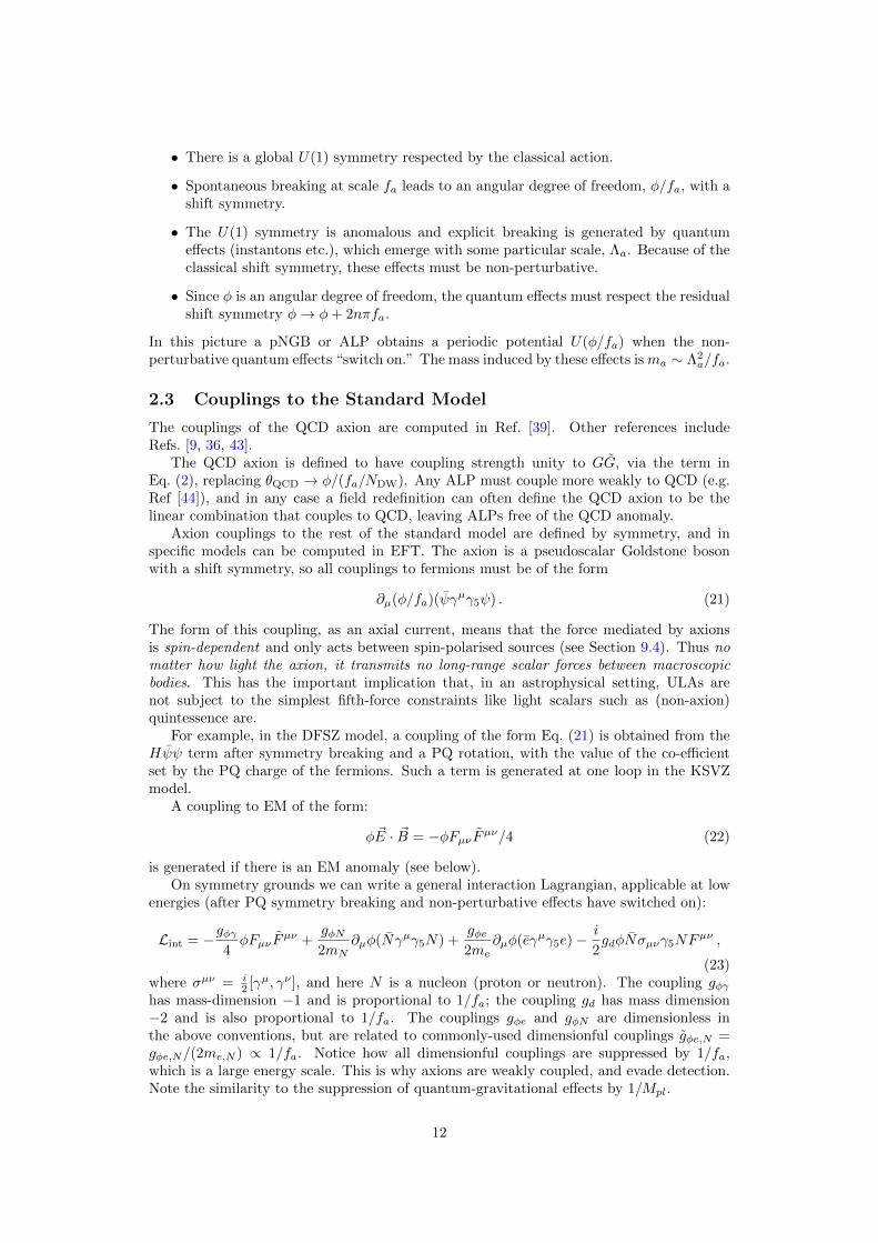
Axion couplings to the rest of the standard model are defined by symmetry, and inspecific models can be computed in EFT. The axion is a pseudoscalar Goldstone bosonwith a shift symmetry, so all couplings to fermions must be of the form

∂µ(φ/fa)(ψγµγ5ψ) . (21)

The form of this coupling, as an axial current, means that the force mediated by axionsis spin-dependent and only acts between spin-polarised sources (see Section 9.4). Thus nomatter how light the axion, it transmits no long-range scalar forces between macroscopicbodies. This has the important implication that, in an astrophysical setting, ULAs arenot subject to the simplest fifth-force constraints like light scalars such as (non-axion)quintessence are.

For example, in the DFSZ model, a coupling of the form Eq. (21) is obtained from theHψψ term after symmetry breaking and a PQ rotation, with the value of the co-efficientset by the PQ charge of the fermions. Such a term is generated at one loop in the KSVZmodel.

A coupling to EM of the form:

φ~E · ~B = −φFµν Fµν/4 (22)

is generated if there is an EM anomaly (see below).On symmetry grounds we can write a general interaction Lagrangian, applicable at low

energies (after PQ symmetry breaking and non-perturbative effects have switched on):

Lint = −gφγ4φFµν F

µν +gφN2mN

∂µφ(Nγµγ5N) +gφe2me

∂µφ(eγµγ5e)−i

2gdφNσµνγ5NF

µν ,

(23)where σµν = i

2 [γµ, γν ], and here N is a nucleon (proton or neutron). The coupling gφγhas mass-dimension −1 and is proportional to 1/fa; the coupling gd has mass dimension−2 and is also proportional to 1/fa. The couplings gφe and gφN are dimensionless inthe above conventions, but are related to commonly-used dimensionful couplings gφe,N =gφe,N/(2me,N ) ∝ 1/fa. Notice how all dimensionful couplings are suppressed by 1/fa,which is a large energy scale. This is why axions are weakly coupled, and evade detection.Note the similarity to the suppression of quantum-gravitational effects by 1/Mpl.

12

In generic ALP models the couplings to the standard model are taken as free parametersthat and can be very much less than they are in the QCD case if, e.g., they are loopsuppressed, or forbidden on symmetry grounds. In specific models, the couplings of ALPscan be computed (e.g. Refs. [45, 46]).

Expressions for all standard model couplings of the QCD axion can be found in, e.g.Ref. [43] (though the notation differs slightly). The EDM coupling, gd, is discussed inRef. [47]. In this section, we will only discuss the two-photon coupling in detail, followingRef. [36]. We define:

gφγ =αEM

2π(fa/C)cφγ , (24)

where αEM ≈ 1/137 is the EM coupling constant and cφγ is dimensionless. The dimension-less coupling obtains contributions from above the chiral symmetry breaking scale, via theEM anomaly, and below the chiral-symmetry breaking scale, by mixing with the longitudi-nal component of the Z-boson [39]:

cφγ =EC −

2

3· 4 +mu/md

1 +mu/md, (25)

where E is the EM anomaly:E = 2Tr QPQQ2

EM , (26)

and QEM are the EM chargesWe see clearly here how the KSVZ and DFSZ models differ. In KSVZ we only have the

heavy Q fields with PQ charge, and so the value of cφγ is fixed by the EM charge assignedto this field. Model dependence in KSVZ occurs if we introduce additional heavy quarkswith PQ and EM charges. In the DFSZ model, all the standard model fermions carry PQcharges. Model dependence in DFSZ occurs because the coupling depends on the leptonPQ charges, i.e. whether Hu or Hd gives mass to the leptons. If Hu gives mass to theleptons, cφγ also depends on the ratio of Higgs vevs, tanβ = 〈Hu〉/〈Hd〉.

The QCD axion has certain canonical choices for the model dependence. For KSVZ onetakes a single EM neutral Q field. For DFSZ the Hd gives mass to the leptons, allowing forSU(5) unification. For mu/md = 0.6, the couplings are then:

cφγ = −1.92 (KSVZ); cφγ = 0.75 (DFSZ). (27)

2.4 Axions in String Theory

As is well known, string theory requires the existence of more spacetime dimensions thanour usual four: 10 in the case of the critical superstring, and 11 in the case of M-theory [48,49, 50]. The additional spacetime dimensions must be “compactified,” that is, rolled upand made compact, with a small size. Typically, for appropriate phenomenology containingsome unbroken SUSY and chiral matter, the compact manifold must be “Calabi-Yau” [51].The supergravity description of string theory contains antisymmetric tensor fields: forexample, the antisymmetric partner of the metric, BMN , is present in all string theories.

Axions arise as the Kaluza-Klein (KK) zero modes of the antisymmetric tensors on theCalabi-Yau [52]. The number of axions present depends on the topology of the compactmanifold, and in particular is determined by its Hodge numbers. Many Calabi-Yau mani-folds are known to exist, and the distribution peaks for Hodge numbers in the dozens [53],as shown in Fig. 3 for the Kreuzer-Skarke [54] list. Furthermore, axions arising in this wayare massless to all orders in perturbation theory thanks to the higher-dimensional gaugeinvariance. The axions then obtain mass by non-perturbative effects, such as instantons.Thus axions, with symmetry properties similar to those axions in field theory that we havealready discussed, are an extremely generic prediction of string theory, in the low-energy

13

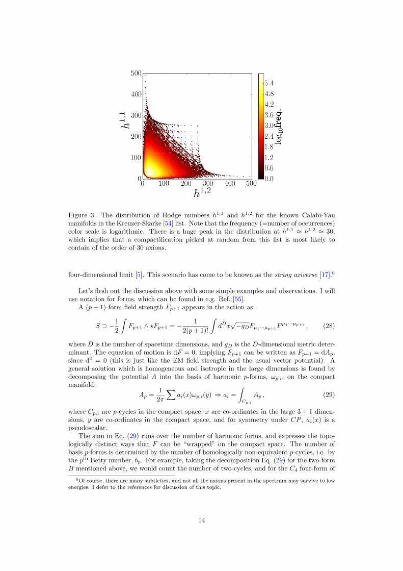
h1,1

h1,2

Figure 3: The distribution of Hodge numbers h1,1 and h1,2 for the known Calabi-Yaumanifolds in the Kreuzer-Skarke [54] list. Note that the frequency (=number of occurrences)color scale is logarithmic. There is a huge peak in the distribution at h1,1 ≈ h1,2 ≈ 30,which implies that a compactification picked at random from this list is most likely tocontain of the order of 30 axions.

four-dimensional limit [5]. This scenario has come to be known as the string axiverse [17].6

Let’s flesh out the discussion above with some simple examples and observations. I willuse notation for forms, which can be found in e.g. Ref. [55].

A (p+ 1)-form field strength Fp+1 appears in the action as:

S ⊃ −1

2

∫Fp+1 ∧ ?Fp+1 = − 1

2(p+ 1)!

∫dDx√−gDFµ1···µp+1

Fµ1···µp+1 , (28)

where D is the number of spacetime dimensions, and gD is the D-dimensional metric deter-minant. The equation of motion is dF = 0, implying Fp+1 can be written as Fp+1 = dAp,since d2 = 0 (this is just like the EM field strength and the usual vector potential). Ageneral solution which is homogeneous and isotropic in the large dimensions is found bydecomposing the potential A into the basis of harmonic p-forms, ωp,i, on the compactmanifold:

Ap =1

2π

∑ai(x)ωp,i(y) ⇒ ai =

∫Cp,i

Ap , (29)

where Cp,i are p-cycles in the compact space, x are co-ordinates in the large 3 + 1 dimen-sions, y are co-ordinates in the compact space, and for symmetry under CP , ai(x) is apseudoscalar.

The sum in Eq. (29) runs over the number of harmonic forms, and expresses the topo-logically distinct ways that F can be “wrapped” on the compact space. The number ofbasis p-forms is determined by the number of homologically non-equivalent p-cycles, i.e. bythe pth Betty number, bp. For example, taking the decomposition Eq. (29) for the two-formB mentioned above, we would count the number of two-cycles, and for the C4 four-form of

6Of course, there are many subtleties, and not all the axions present in the spectrum may survive to lowenergies. I defer to the references for discussion of this topic.

14

Type IIB theory, we would count the number of four-cycles.7 For a Calabi-Yau three-fold(three complex dimensions, six real dimensions), all the bp are determined by the two Hodgenumbers h1,1 and h1,2 (see, e.g., Chapter 9 of Ref. [50], and Fig. 3 above).

The axions of Eq. (29) are closed string axions. Each closed string axion is partneredinto a complex field zi = σi + iai where σi is a scalar modulus (saxion) field controllingthe size of the corresponding p-cycle. The moduli come from KK reduction of the Ricciscalar as usual, and their pairing with axions is a consequence of SUSY, which demandsthe existence of the appropriate form fields in supergravity. Open string axions also existin string theory, and are more like the field theory axions we discussed previously. Openstring axions live on spacetime filling branes supporting gauge theories and are the phasesof matter fields, ϕ, which break global PQ symmetries. Open string axions might be relatedto closed string axions by gauge/gravity duality [56, 57].

We have just seen the basics of how string theory gives rise to axions and moduli, thenumber of which is determined by the topology of the compact space. Next we must askwhat determines the spectrum of axion masses and decay constants.

After KK reduction of Eq. (28) the ai(x) fields are found to be massless, i.e. there areonly kinetic terms for them in the action, implying a shift symmetry. The shift symmetrydescends from the higher-dimensional gauge invariance of F , and so is protected to allorders in perturbation theory.

In Type IIB theory, the axion kinetic term resulting from KK reduction of the action forthe C4 four-form potential is (for the full axion action in Type IIB theory, see e.g. Ref. [14])

S ⊃ −1

8

∫daiKij ∧ ?daj , (30)

where Kij is the Kahler metric,

Kij =∂2K

∂σi∂σj, (31)

and K is the Kahler potential, which depends on the moduli. KK reduction kineticallymixes the axions and couples them to the moduli via the Kahler metric. Canonicallynormalizing the kinetic terms and diagonalizing the Kahler metric, we see that it is themoduli that determine the axion decay constants, since the canonical kinetic term is Lkin. =−f2

a,i(∂ai)2/2. In particular we have that, parametrically,8

fa,i ∼Mpl

σi.Mpl , (32)

where the dimensionless modulus σi measures the volume of the corresponding p-cycle instring units, i.e. σi = Voli/l

ps , for string length ls. The volume should be larger than the

string scale in order for the effective field theory description to be valid, giving the inequality.This may be related to be a general feature, known as the “weak gravity conjecture,”following from properties of black holes [59].9 We return to this question in the context ofinflation in Section 7.2.

7Take a simple example in non-string theory jargon. Imagine a vector field, Aµ with field strength Fµνin 3+1 large dimensions, and a two dimensional compact space in the shape of a doughnut (or two-torus).There are two distinct ways the vector field can wrap the doughnut: along the tube, or all the way around.These are the distinct one-cycles of the torus. The vector field has co-ordinates in the large dimensions also,but if these are to be homogeneous and isotropic, the only dependence can be as a (pseudo)scalar expressinghow wrapping varies from place to place. The two fields necessary are the axions: the KK zero-modes ofthe A field wrapped on the one-cycles.

8I have assumed that the size of the cycle is of order the size of the manifold. See Refs. [5, 58] for moredetails.

9The relation of the conjecture to axion decay constants is only well formulated in the case of a singleaxion. Consider, for example, the two axion model of Ref. [60] has a decay constant ∼ 3.25Mpl. Oursimplistic description here has ignored the phenomenon of alignment [61, 62].

15

Axions in string theory can obtain potentials from a variety of non-perturbative ef-fects (see e.g. Refs. [5, 17, 58, 63]). In general, instantons provide a contribution to thesuperpotential, W for the axion field a = φ/fa:

W = M3e−Sinst.+ia , (33)

where Sinst. is the instanton action and M is the scale of instanton physics, which in stringtheory may be the Planck scale. If SUSY is broken at a scale mSUSY then the axion potentialat low energies is

V (φ) = Λ4a[1− cos(φ/fa)] with Λ4

a = m2SUSYM

2ple−Sinst. . (34)

A non-Abelian gauge group has instantons with action given by Eq. (20). In stringtheory, the moduli couple to the gauge kinetic term for a non-Abelian group realized bya stack of D-branes wrapping the corresponding cycle, and the gauge coupling g2 ∝ 1/σ(this occurs e.g. in Type IIB theory for gauge theory on a stack of D7 branes filling 3+1spacetime and wrapped on the same four-cycles as C4). Thus, if an axion obtains massfrom these instantons as above, we find that the axion mass scales exponentially with thecycle volumes:

m2a ∼

µ4

f2a

e−#σi , (35)

where µ is a hard scale. In general, from the above, we expect µ =√mSUSYMpl. If the

moduli are stabilised by perturbative SUSY breaking effects giving mσ ∼ mSUSY ma

then the moduli can be set to constant values at late times in cosmology and the axionmass will be a constant (for dynamical moduli as dark energy, see Refs. [64, 65]).

The two observations, Eqs. (32,35), form the key basis for the phenomenology of theaxiverse. Thanks to the exponential scaling of the potential energy scale with respect tothe moduli, string axions will have masses spanning many orders of magnitude. The axiondecay constants will (generally) be parametrically smaller than the Planck scale, and areexpected to span only a small range of scales due to the power-law scaling with the moduli.

Let’s end this discussion with a few examples of explicit string theory constructionsdisplaying the above properties. The so-called “model independent axion” in heteroticstring theory emerges from compactification of BMN on two-cycles. It has decay constantfa = αGUTMpl/2

√2π and the shift symmetry of the axions is broken by wrapped NS-

5 branes with Sinst. = 2π/αGUT [5]. Gauge coupling unification at αGUT = 1/25 givesfa ∼ 1.1× 1016 GeV.

The M-theory axiverse [66] is realized as a compactification of M-theory on a G2 mani-fold, with axions arising from the number of three-cycles. The G2 volume is small, fixing oneheavy string-scale axion by leading non-perturbative effects, and giving fa ≈ 1016 GeV. Theremaining axions obtain potentials from higher order effects, and are hierarchically lighter.Fixing the GUT coupling requires that an additional axion take a mass ma,GUT ≈ 10−15 eV.The other axions in the theory will be distributed around these characteristic values ac-cording to the scalings we have discussed.

The Type IIB axiverse [67] is a LARGE volume Calabi-Yau compactification [68, 69],with axions arising from C4 as discussed above. At least two axions are required in thisscenario, one of which is the almost-massless volume-axion associated to the exponentiallylarge volume-modulus, and the other is again associated to the GUT coupling. The volume,V, is exponentially large in string units and gives the decay constant of the volume-axionas fa ≈ 1010 GeV. Other light axions are associated to perturbatively fixed moduli, sincethey must obtain masses only from higher order effects. Larger values of the effectivedecay constant for very light axions with ma ∼ H0 can be achieved in this scenario byalignment [70].

16

3 Production and Initial Conditions

3.1 Symmetry Breaking and Non-Perturbative Physics

Let’s briefly review the general picture for axions given in the previous section, highlightinghow this is relevant to axion cosmology in the very early Universe. Two important physicalprocesses determine this behaviour. Symmetry breaking occurs at some high scale, fa,and establishes the axion as a Goldstone boson. Next, non-perturbative physics becomesrelevant, at some temperature TNP fa, and provides a potential for the axion.

Giving substance to this chain of events: the axion field, φ, is related to the angulardegree of freedom of a complex scalar, ϕ = χeiφ/fa . The radial field, χ, obtains the vev〈χ〉 = fa/

√2 when a global U(1) symmetry is broken (see Fig. 2). The field χ is heavy, and

fa is the PQ symmetry breaking scale. The axion is the Goldstone boson of this brokensymmetry , and possesses a shift symmetry, φ→ φ+const., making it massless to all ordersin perturbation theory. Non-perturbative effects, for example instantons, “switch on” atsome particular energy scale and break this shift symmetry, inducing a potential for theaxion, V (φ). The potential must, however, respect the residual discrete shift symmetry,φ → φ + 2nπfa/NDW, for some integer n, which remains because the axion is still theangular degree of freedom of a complex field. The potential is therefore periodic.

The scale of non-perturbative physics is Λa and the potential can be written as V (φ) =Λ4aU(φ/fa), where U(x) is periodic, and therefore possesses at least one minimum and one

maximum on the interval x ∈ [−π, π]. We can choose the origin in field space such thatU(x) has its minimum at x = 0.10 It is common practice to assume a solution to thecosmological constant problem such that the minimum is also obtained at U(0) = 0 (seeSection 7.1 for further discussion). A particularly simple choice for the potential is then

V (φ) = Λ4a

[1− cos

(NDWφ

fa

)], (36)

where NDW is an integer, which unless otherwise stated I will set equal to unity. I stress thatthe potential Eq. (36) is not unique and without detailed knowledge of the non-perturbativephysics it cannot be predicted. For example, so-called “higher order instanton corrections”might appear, as cosn φ/fa (see e.g. Ref. [71]). The form of the potential given by Eq. (36)is, however, a useful benchmark for considering the form of axion self-interactions.

We can study axions in a model-independent way if we consider only small, φ < fa,displacements from the potential minimum. In this case, the potential can be expanded asa Taylor series. The dominant term is the mass term:

V (φ) ≈ 1

2m2aφ

2 , (37)

where m2a = Λ4

a/f2a . The symmetry breaking scale is typically rather high, while the non-

perturbative scale is lower. The axion mass is thus parametrically small.Let’s consider some possible values for these scales. The QCD axion (see Section 2.1)

is the canonical example, where we have that Λ4a ≈ Λ3

QCDmu with ΛQCD ≈ 200 MeV and

mu the u-quark mass, and 109 Gev . fa . 1017 GeV. The lower limit on fa comes fromsupernova cooling [72, 73] (see Section 9.1), while the upper limit comes from black holesuperradiance [74] (BHSR, see Section 8.1). This leads to an axion mass in the range4× 10−10 eV . ma,QCD . 4× 10−2 eV.

In string theory models (see Section 2.4), things are much more uncertain. The decayconstant typically takes values near the GUT scale, fa ∼ 1016 GeV [5], though lower valuesof fa ∼ 1010−12 GeV are possible [67]. In specific, controlled, examples one always finds

10When x 6= 0 is associated to the breaking of CP symmetry, as is the case for the QCD axion, a theoremof Vafa and Witten [23] guarantees that the induced potential has a minimum at the CP -conserving valuex = 0.

17

fa .Mpl for individual axion fields. The “weak gravity conjecture” places some constraintson realising super-Planckian decay constants within quantum gravity [59].11 The potentialenergy scale in string models depends exponentially on details of the compactification,and large hierarchies between the non-perturbative scale and the string scale can easily beachieved. Explicitly, Λa ∼ µe−σ, where µ is the hard non-perturbative scale (e.g. SUSYbreaking), and σ is a modulus field describing the size of the compact dimensions in stringunits: small changes in σ produce large changes in Λa for fixed µ. String models areexpected to possess a large number of axions, with each axion associated to a differentmodulus. String axions thus have a mass spectrum spanning a vast number of orders ofmagnitude from the string scale down to zero. In particular, string models can realise aspectrum such as Eq. (1).

The axion mass is protected from quantum corrections, since these all break the un-derlying shift symmetry and must come suppressed by powers of fa. For the same reason,self-interactions and interactions with standard model fields are also suppressed by powersof fa (for the self-interactions, we can see this easily by expanding the cosine potential tohigher orders). This renders the axion a light, weakly interacting, long-lived particle. Theseproperties are protected by a symmetry and as such the axion provides a natural candidateto address cosmological problems that can be solved using a light scalar field. Axions canbe used to drive inflation, to provide DM, and to provide DE.

Taking only the mass term from the potential for simplicity, the homogeneous componentof the axion field obeys the equation

φ+ 3Hφ+m2aφ = 0 . (38)

This is the equation of a simple harmonic oscillator with time dependent friction determinedby the Friedmann equations, Eqs. (B2). In general, the axion mass will be temperaturedependent, as the non-perturbative effects switch on. We will study this equation in detailin Section 4. An important stage in the evolution of the axion field is the transition formover-damped to under-damped motion, which occurs when H ∼ ma, and the axion fieldbegins oscillating.

3.2 The Axion Field During Inflation

This section refers explicitly to DM axions as a spectator fields during inflation.12 Inflationdriven by an axion field is discussed in Sec. 7.2.

The temperature of the Universe during inflation is given by the Gibbons-Hawking [81]temperature (Hawking radiation emitted from the de-Sitter horizon):

TI =HI

2π, (39)

where HI is the inflationary Hubble scale. This temperature determines whether the PQsymmetry is broken or unbroken during inflation, with each scenario giving rise to a differentcosmology.

The inflationary Hubble scale is tied to the value of the tensor-to-scalar ratio, rT :

HI

2π= Mpl

√AsrT /8 . (40)

11Collective behaviour of multiple axion fields further complicates matters. We will return to this topicin Section 7.2. A large literature surrounds the question of super-Planckian axions in string theory, see e.g.Refs. [75, 71, 76, 77, 78, 79, 80], and references therein.

12I assume a standard, single-field, slow-roll inflationary model throughout these notes, as it gives us aconcrete setting for performing calculations and comparing to data. I further assume (for the most part)that the Universe is radiation dominated from the end of inflation, and in particular when V (φ) switcheson. The general principles, however, can be used as a guide for computing in non-standard cosmologies.The important aspects to consider are: when does symmetry breaking occur with respect to the epochwhen initial conditions are set; what is the energy scale at which initial conditions are set; what dominatesthe energy density when the non-perturbative physics giving rise to V (φ) becomes relevant?

18

where As is the scalar amplitude. Ever since the observation of the first acoustic peak inthe CMB [82, 83, 84], we have known that rT < 1 and that cosmological fluctuations aredominantly scalar and adiabatic, with

√As ∼ 10−5 first measured by COBE [85]. This sets,

very roughly, HI . 1014 GeV. The most up-to-date constraints come from the combinedanalysis of Planck and BICEP2 [86], which give As = 2.20× 10−9, rT < 0.12 and thus

HI

2π< 1.4× 1013 GeV . (41)

High scale single-field slow-roll inflation has observably large tensor modes, rT & 10−3, andrequires super-Planckian motion of the inflaton [87]. We will discuss the importance ofCMB tensor modes to axion phenomenology in more detail in Section 5.4.

3.2.1 PQ symmetry unbroken during inflation, fa < HI/2π

This scenario occurs when fa < HI/2π. A large misalignment population of ULA DM (ourmain focus in these notes) requires fa ∼ 1016 GeV, and so this scenario is irrelevant to thatmodel. This is an important scenario for the QCD axion, however, since it applies to theADMX [88] sensitivity range of fa ∼ 1012 GeV in the case of high scale standard inflation.

During inflation, fluctuations induced by the Gibbons-Hawking temperature are largeenough that the U(1) symmetry is unbroken and ϕ has zero vev. After inflation, thesymmetry breaks when the radiation temperature drops below fa. At this point, χ obtainsa vev and each causally disconnected patch picks a different value for φ/fa = θPQ. Sincethe decay constant is larger than the scale of non-perturbative physics, the axion has nopotential at this time, and θPQ thus has no preferred value. Therefore, in each Hubblepatch θPQ is drawn at random from a uniform distribution on [−π, π]. The horizon sizeR ∼ 1/H when the PQ symmetry is broken. The symmetry is broken in the early Universe,and the present day Universe is made up of many patches that had different initial valuesof θPQ.

Given the θPQ distribution, it is possible to compute the average value of the square ofthe axion field, 〈φ2〉. As we will see later, this value fixes the axion relic density producedby vacuum realignment in this scenario (see Sections 3.3 and 4.3). However, it is clear thatthere are O(1) fluctuations in the axion field from place to place on scales of order thehorizon size when non-perturbative effects switch on (R ∼ 10 pc today for the QCD axion).These large fluctuations have been conjectured to give rise to so-called “axion miniclusters”[89]. Fluctuations of this type are non-adiabatic, but are not scale invariant and give riseto additional power only on scales sub-horizon at PQ symmetry breaking.

The breaking of global symmetries gives rise to topological defects. A broken U(1)creates axion strings, while having NDW > 1 in Eq. (36), as in the DFSZ QCD axion model,gives rise to domain walls. When the PQ symmetry breaks after inflation, a number of suchdefects will remain in the present Universe. Domain walls, if stable, are phenomenologicallydisastrous, since their energy density scales like 1/a2 and they can quickly dominate theenergy density of the Universe [90]. They can be avoided if NDW = 1 in Eq. (36), whichis possible in the KSVZ axion model, although other mechanisms to avoid their disastrousconsequences exist (e.g. Ref. [91]). Cosmic strings have a host of additional phenomenology.Perturbations seeded by strings and the decay of domain walls may lead to the existenceof heavy axion clumps [92]. For our purposes, the most important impact of axion stringsis that their decay can source a population of relic axions, which is discussed below.

The important phenomenological aspects of the unbroken PQ scenario are:

• The average (background) initial misalignment angle is not a free parameter: 〈θ2a,i〉 =

π2/3.

• Phase transition relics are present. Their consequences must be dealt with.

• Existence of axion miniclusters?

19

3.2.2 PQ symmetry broken during inflation, fa > HI/2π

This scenario occurs when fa > HI/2π. It is particularly relevant for GUT scale axions,and all axion DM models combined with low-scale inflation.

As in the previous scenario, PQ symmetry breaking establishes causally disconnectedpatches with different values of θPQ, and produces topological defects. However, the rapidexpansion during inflation dilutes all the phase transition relics away.13 It also stretches outeach patch of θPQ, so that our current Hubble volume began life at the end of inflation witha single uniform value of θPQ everywhere. This initial value of θPQ is completely random.It is again drawn from a uniform distribution, but the existence of many different Hubblepatches means that values of θPQ arbitrarily close to zero or π cannot be excluded, excepton grounds of taste or anthropics.

Fluctuations in θPQ, which later seed structure formation with axion DM, are generatedin two different ways in this scenario. Firstly, as we will show in Section 4.4, the axion fieldhas a gravitational Jeans instability. Axion DM will fall into the potential wells establishedby photons in the radiation era (which were in turn established by quantum fluctuationsduring inflation). This leads to adiabatic fluctuations.

The second source of axion fluctuations are inflationary isocurvature modes. When thePQ symmetry is broken during inflation, the axion exists as a massless field (or in any case,one with ma HI). All massless fields in de Sitter space undergo quantum fluctuationswith amplitude

δφ =HI

2π. (42)

The amplitude of the power spectrum of these perturbations is proportional to rT . In deSitter space, the power spectrum would be scale invariant. Slow roll inflation imparts a redtilt. The isocurvature spectral index is the same as the tensor spectral index, and is alsofixed by HI via inflationary consistency conditions.

Just like tensor modes, DM isocurvature perturbations of this type do not give rise toa large first acoustic peak in the CMB, and are thus constrained to be sub-dominant. Thelatest Planck constraints give AI/As < 0.038 [96]. As we will discuss in detail in Section 5.4,this typically forbids the compatibility of fa & 1011 GeV axion DM and an observably largerT .

Isocurvature perturbations also give rise to a backreaction contribution to the homoge-neous field displacement (see e.g. Ref. [97])

〈φ2i 〉 = f2

aθ2a,i + 〈δφ2〉 ,

= f2aθ

2a,i + (HI/2π)2 . (43)

The backreaction sets a minimum value to the misalignment population of axions that canbe significant in high scale inflation for heavier ALPs, ma & 10−12 eV, and the QCD axion.

The important phenomenological aspects of the broken PQ scenario are:

• The average (background) initial misalignment angle is a free parameter, with a min-imum value fixed by backreaction.

• Isocurvature perturbations are produced. Their consequences must be dealt with.

• Use as a probe of inflation?

3.3 Cosmological Populations of Axions

The relic density of axions is ρa = Ωaρcrit. In cosmology we often discuss the physicaldensity, Ωah

2, by factoring out the dimensionless Hubble parameter, h, from the criticaldensity. This gives ρa = Ωah

2 × (3.0× 10−3 eV)4.

13Recall that one of the original motivations for inflation was as a solution to the monopoloe problem ofGUT theories [93, 94, 95].

20

A relic axion population can be produced in a number of different ways. The fourprinciple mechanisms are:

• Decay product of parent particle.

• Decay product of topological defect.

• Thermal population from the radiation bath.

• Vacuum Realignment.

I will discuss the first three briefly here, but leave most of the details to the references.Vacuum realignment is discussed in detail in Section 4.3.

3.3.1 Decay Product of Parent Particle

A massive particle, X, with mX > ma, is coupled to the axion field, and decays, producinga population of relativistic axions. If the decay occurs after the axions have decoupled fromthe standard model then they remain relativistic throughout the history of the Universe.In this case, axions are dark radiation (DR). In cosmology, DR is parameterised via the“effective number of relativistic neutrinos,” Neff , defined as:

ρr = ργ

[1 +

7

8

(4

11

)4/3

Neff

]. (44)

Recall that three species of massless neutrinos in the standard model of particle physicscontribute Neff = 3.04, the additional 0.04 being contributed by heating after e+e− anni-hilation [98].

Assuming instantaneous decay of the parent particle when it dominates the energydensity of the Universe gives:14

∆Neff =43

7

(10.75

g?S(Tr)

)1/3Ba

1−Ba, (45)

where Tr is the reheating temperature of the decay of the parent particle, Ba is the branchingratio to axions, and g?S(T ) is the entropic degrees of freedom. The evolution of g?,S(T ) inthe standard model can be computed or can be looked up, e.g. in the Review of ParticlePhysics [21].

DR can affect the CMB in a number of ways; for a concise description, see Ref. [103].If we hold the angular size of the sound horizon fixed (compensating the change in matterradiation equality with a different Hubble constant or DE density), the main effect of DRis to cause additional damping of the high-multipole acoustic peaks in the CMB.15 Thisdamping tail is well measured by Planck, ACT and SPT, giving Neff = 3.15 ± 0.23 froma representative combination of CMB data [105]. Neff is also constrained by big bangnucleosynthesis (BBN, again see Ref. [105]). Whether this should be combined with theCMB constraint depends on whether the decay producing the axions occurred before orafter BBN. An important point to note about neutrino constraints form the CMB is thatthey do not care whether the DR is a boson or a fermion. We discuss more consequencesof axionic dark radiation in Section 9.7.

A scenario in which axions are produced in this way arises in models with SUSY and ex-tra dimensions. The DR “cosmic axion background” is thus considered a generic prediction

14If the parent particle does not dominate the energy density of the Universe when it decays, thenunder certain circumstances it may act as a curvaton [99, 100, 101] and sources correlated isocurvatureperturbations, which are also constrained by the CMB. See, e.g., Ref. [102].

15Recent constraints on Neff in Ref. [104] have separated the damping tail effect from the neutrinoanisotropic stress, which changes the angular scale of the higher acoustic peaks (see also constraints onneutrino viscosity in Ref. [105]).

21

of many string and M-theory compactifications, and it has a rich phenomenology (see e.g.Refs. [66, 106, 107, 108] and Sections 9.7 and 9.8.2 of this review). In these models, a Kahlermodulus, σ, of the compact space comes to dominate the energy density of the Universeafter inflation, leading to an additional matter dominated era and a non-thermal history.The modulus must decay and reheat the Universe to a temperature above TBBN ∼ 3 MeV,since BBN does not occur successfully in a matter dominated universe.16 Moduli are gravi-tationally coupled and are therfore expected to have comparable branching ratios to hiddenand visible sectors, and in particular have a large branching ratio to axions, since axions arepartnered to moduli by SUSY. The modulus decay rate is given by its mass, Γσ ∼ m3

σ/M2pl

and it decays when H ∼ Γσ. Decay before BBN requires mσ & 10 TeV. Moduli are thusmuch heavier than axions, and their decay produces a sizeable relativistic axion population,surviving from before BBN until today.

3.3.2 Decay Product of Topological Defect

The breaking of global symmetries leads to the formation of topological defects. In thecase of a global U(1) symmetry, like the PQ symmetry, this means global (axionic) stringsand (if NDW > 1) domain walls. In the broken PQ scenario, topological defects and theirdecay products are inflated away, and can be ignored, so here we focus on the unbrokenPQ scenario. Axion strings decay, producing a population of cold axions, which we discussbelow. The energy density in domain walls scales like ρDW ∼ a−2 and can quickly domi-nate the energy density of the Universe, with phenomenologically disastrous results. ThusNDW > 1 models (like the DFSZ model) typically require the broken PQ scenario, or someother mechanism to remove the domain walls (see e.g. Ref. [91] and references therein). Inthis Section I give only the briefest overview of axion production from topological defects:see e.g. Refs. [43, 8, 111] for more details.

Let’s focus on strings. Strings are formed by the “winding” of the θ angle. The valueof the θ angle is set independently at each point in space when the PQ symmetry breaks.The Goldstone nature of θ homogenizes this value in each horizon volume. As the hori-zon grows, the homogenized area grows. However, in different horizon volumes, θ will bedifferent. Then, if the θ angle undergoes a winding around any given point in space, themapping between θ and the spatial co-ordinates does not allow a continuous unwinding,leading to a string-like topological defect along the length of the region enclosed by thewinding. Formation of topological defects in cosmology in this manner is known as theKibble mechanism [112].

Strings in cosmology enter into a “scaling solution,” caused by strings within any horizonvolume cutting themselves into loops. During the radiation dominated epoch, this requiresthe string energy density to scale as:

ρstring ∝ µstring/t2 , µstring ∼ f2

a ln(fad) , (46)

where µstring is the energy per unit length of the axion string, and d the characteristicdistance between strings. For global strings, this scaling symmetry is maintained by thecontinuous emission of axions. The change in the number density of axions, na, per entropydensity, s, per Hubble time, required for this is [43]:

∆(na/s) ∼µstringt

2

ωT 3∆(Ht) (47)

where ω is the average energy of the radiated axion.Recall from Eq. (38) that the axion field begins oscillating when ma ∼ H, which occurs

at a temperature Tosc., and depends on the temperature evolution of the axion mass (wediscuss this in more detail for the misalignment population of axions in Section 4). When

16This is the “cosmological moduli problem,” see e.g. Refs. [109, 110].

22

oscillations commence, axion strings become the boundaries of domain walls connected bystrings. For NDW = 1, these walls can be “unzipped” by the strings (as explained inRef. [8]), and the decay of the topological defects is complete. Therefore, the total numberof axions produced by string decay in a comoving volume is given by the integral of Eq. (47)from the time of the PQ phase transition at T = fa up to Tosc:

nas∼∫ fa

Tosc

µstringdT

ω(T )M2pl

. (48)

Axions produced by string decay are dominated by the low-frequency modes, makingthem non-relativistic and contributing as CDM to the cosmic energy budget. Accuratecomputation of the relic density requires numerical simulation of the PQ phase transitionand decay of axion strings in order to determine the energy spectrum, ω(T ). Results ofsuch simulations are commonly expressed as the ratio of axion energy density produced bytopological defect decay compared to that produced by misalignment:

Ωah2 = Ωa,mish

2(1 + αdec.) . (49)

For the specific case of the QCD axion, with known temperature dependence of themass, the value of αdec is calculated.17 There is a long-standing controversy over what thevalue of αdec. should be, with quoted values ranging from 0.16 to 186 [114, 115, 116, 117],with the true value possibly lying somewhere in between [111].

The uncertainty arises from the form of the spectrum ω. If the radiated axions havethe longest wavelengths possible, of order the horizon, then ω(t) ∼ t−1 [114], while if thespectrum ∼ 1/k (cut off at the horizon and the string size) then ω(t) ∼ ln(fat)t

−1 [115].These stem from different assumptions about simulating strings. For the QCD axion mass-temperature relation, this factor of ln(fatosc) ∼ 70, with the enhancement occurring for thecase where ω ∼ t−1 (accounting for the t dependence of µ with d ∼ t). The modern directsimulation of the PQ field yields the somewhat intermediate result of Ref [111].

This is clearly a very important area of uncertainty in models of high scale inflationand intermediate scale axions that could have consequences for direct detection of the QCDaxion. If decay products from topological defects can produce a relic density larger thanmisalignment (αdec. 1), then axions with fa as low as 109 GeV could be relevant DMcandidates (see Section 4.3.2 for quantitative details). Ultimately, if αdec. were too large,then QCD axion DM would be excluded by stellar astrophysics (see Section 9.1). Directdetection of low-fa axions is outside the reach of ADMX, but may be possible with e.g.open resonator searches (see Section 9.5.1).

Topological defects also source CMB fluctuations (e.g. Ref. [118]). A cosmic stringnetwork generates power on all sub-horizon scales [119]. Therefore, axion strings onlygenerate power on scales of order the horizon size at string decay. This scale is small, andis not constrained by the CMB power spectrum, but axion strings may source additionalpower on minicluster scales.

3.3.3 Thermal Production

If axions are in thermal contact with the standard model radiation, then mutual produc-tion and annihilation can lead to a thermal relic population of axions, just as for massivestandard model neutrinos and WIMPs. The couplings of an axion to the standard modelare only specified in the case of the QCD axion. Furthermore, generic ALPs are often more

17As we will show shortly, the contribution from misalignment, Ωa,mish2, has a particular scaling with fa

for the QCD axion. Quoting a constant value for αdec. in the parameterisation Eq. (49) assumes the samescaling with fa for the population produced by topological defect decay. Ref. [113] show slightly differentscalings, but argue that the uncertainty due to mass-dependence is sub-dominant to other uncertainties inthe string calculation.

23

weakly coupled to the standard model, or at least to QCD, than the QCD axion. For thesereasons, we will consider only the thermal population of the QCD axion.

Axions are produced from the standard model plasma by pion scattering, and decouplewhen the rate for the π+π → π+a process drops below the Hubble rate. The thermal axionabundance is fixed by freeze-out at the decoupling temperature (see, e.g. Ref. [43]), witha larger relic density for lower decoupling temperatures. The number density in thermalaxions, na, relative to the photon number density, nγ is given by

na =nγ2

g?,S(T0)

g?,S(TD), (50)

with TD the decoupling temperature, and T0 the CMB temperature today. See Ref. [120]for a more complete formula and a computation involving all relevant standard modelproduction channels. Thermal axions contribute to the effective number of neutrinos as∆Neff ≈ 0.0264na/na,eq ≈ 10na, with na,eq the thermal equilibrium number density.

Since axion couplings scale inversely with fa, only low fa (higher mass) thermally pro-duced axions can contribute a significant amount to the energy budget of the Universe.Thermal populations are significant for ma & 0.15 eV, when decoupling occurs after theQCD phase transition (recall that g?,S reduces dramatically after the QCD phase transi-tion, diluting the abundance of particles produced before it). For the QCD axion respectingfa & 109 GeV, as suggested by stellar cooling constraints (ses Section 9.1), the thermal pop-ulation is negligible.

Thermal axions produced in this way are relativistic as long as TD > ma. Once de-coupled the axion temperature, Ta, redshifts independently from the standard model tem-perature, and the axions become non-relativistic when Ta < ma. Thermal axions behavecosmologically in a manner similar to massive neutrinos, and contribute as hot DM, sup-pressing cosmological structure formation below the free-streaming scale (see Section 4.4.5).Assuming a standard thermal history, current CMB limits from Planck on axion hot DMconstrain ma < 0.529 → 0.67 eV at 95% confidence [121, 122, 123] (for older limits fromdifferent datasets including large scale structure and WMAP, see Refs. [124, 125, 126, 127]).AFuture galaxy redshift surveys will be sensitive enough to detect a thermal axion popu-lation for all ma ≥ 0.15 eV [128]. Relaxing the assumption of a standard thermal historyand introducing an early matter-dominated phase and low temperature reheating relaxesthe bound on thermal axions, allowing masses as large as a keV [129].

3.3.4 Vacuum Realignment

The process of vacuum realignment is a model independent production mode for axions, alsoknown as the misalignment mechanism. It relies only on their defining properties (beingassociated to spontaneous symmetry breaking, and being a pNGB), and depends only ongravitational (and to some extent self-) interactions. This production mode is our primaryfocus, and is discussed in detail in Section 4.3.

4 The Cosmological Axion Field

If axions are to have observable effects on cosmology, they must contribute an appreciableamount to the energy density of the Universe. Since the axion mass is so small, this implieslarge occupation numbers. In this case, axions can be modelled by solving the classical fieldequations of a condensate. This condensate can have excited states carrying energy andmomentum, and indeed it will. There is nothing more mysterious here than using Maxwell’sequations to describe the behaviour of electric and magnetic fields. It is also the standardway that scalar field models of inflation and DE are treated.

It is a separate question to ask whether axions form a Bose-Einstein condensate (BEC),and even to define a “BEC” in a cosmological context, where we are certainly not in the

24

ground state. I comment briefly on this in Section 4.7. The results I present below arevalid whenever the classical field equations hold, and do not assume BEC occurs (exceptto the extent that it is captured by the classical field equations). Many of the resultsbelow also apply to other models of scalar field DM at late times (when oscillations abouta quadratic minimum are the only important aspect), though the early time cosmology canbe markedly different (e.g. complex fields in Ref. [130], which have equation of state w = 1at early times).

4.1 Action and Energy Momentum Tensor

The action for a minimally coupled real scalar field in General Relativity is:

Sφ =

∫d4x√−g

[−1

2(∂φ)2 − V (φ)

]. (51)

For an axion, this action is only valid after symmetry breaking, and after non-perturbativeeffects have switched on. Before non-perturbative effects have switched on, the axion ismassless. Non-perturbative effects do not switch on instantaneously, either, and time (tem-perature) dependence of the potential can be important. We discuss this shortly, in Sec-tion 4.3.

Varying the action with respect to φ gives the equation of motion

φ− ∂V

∂φ= 0 , (52)

where the D’Alembertian is

=1√−g ∂µ(

√−ggµν∂ν) . (53)

Varying the action with respect to the metric gives the energy momentum tensor

Tµν = gµα∂αφ∂νφ−δµν2

[gαβ∂αφ∂βφ+ 2V (φ)] . (54)

As we will show below, there are certain limits in which the axion field behaves as afluid. See Appendix D for useful definitions for the components of the energy momentumtensor in the fluid case.

4.2 Background Evolution

The background cosmology is defined in Appendix C. Computing the D’Alembertian forthe FRW metric and taking V = m2

aφ2/2, the axion equation of motion is:

φ+ 3Hφ+m2aφ = 0 . (55)

The background energy density and pressure of the axion field are:

ρa =1

2φ2 +

1

2m2aφ

2 , (56)

Pa =1

2φ2 − 1

2m2aφ

2 . (57)

When the universe is matter or radiation dominated the scale factor evolves as a powerlaw, a ∝ tp. In this case, Eq. (55) has an exact solution:

φ = a−3/2(t/ti)1/2[C1Jn(mat) + C2Yn(mat)] , (58)

25

where n = (3p − 1)/2, Jn(x), Yn(x) are Bessel functions of the first and second kind,and ti is the initial time. The dimensionful coefficients C1 and C2 are determined by theinitial conditions. For axions in the vacuum realigment mode, the initial conditions are welldefined when H(ti) ma:

φ(ti) = faθa,i , φ(ti) = 0 . (59)

When matter and radiation are both important, such as near matter-radiation equal-ity,18 or when the axion field can itself dominate the energy density, Eq. (55) must besolved either by approximation or numerically. In the case of axion DM produced by themisalignment mechanism, the most useful approximation to solve Eq. (55) is the WKBapproximation.

4.3 Misalignment Production of DM Axions

The misalignment production of DM axions can be computed given the initial conditions ofEq. (59). At symmetry breaking the Hubble rate is much larger than the axion mass, andthe field is overdamped. This sets φ = 0 initially. The homogeneous value of the field isspecified by the scenario for when symmetry breaking occurs with respect to inflation. Theterm “misalignment” refers to this scenario where there is a coherent initial displacementof the axion field, and “vacuum realignment” to the process by which this value relaxes tothe potential minimum.

An important buzz-word to remember about the misalignment production of DM axionsis that it is non-thermal.

4.3.1 Axion-Like Particles

Let’s begin with the simple case of an ALP. Given ignorance of the non-perturbative physics,I will describe such an axion only by its mass, which I take to be constant in time. Thegeneral picture described here applies to the QCD axion also. The validity of the constantmass assumption will be discussed later in this subsection.

The initial condition φ = 0 fixes the relative values of C1 and C2 in the exact solution tothe background evolution, Eq. (58). The equation of motion is linear, and so the initial fieldvalue can be scaled out. Fig. 4 shows the evolution of the axion field, Hubble rate, axionequation of state, and the axion energy density for the solution Eq. (58) in a radiation-dominated universe (p = 1/2), with arbitrary normalization of all dimensionful parameters.The scale factor is shown relative to the initial value, ai.

At early times when H > ma, the axion field is overdamped and is frozen at its initialvalue by Hubble friction. The equation of state at early times is wa = −1, and the axionbehaves as a contribution to the vacuum energy. This is why axions can serve as modelsfor DE and inflation. All other components of the Universe scale as a to some negativepower. If the axion can come to dominate the energy density while it is still overdampedwith wa < −1/3, it can drive a period of accelerated expansion. The length of this perioddepends on the ratio H/ma when the axion comes to dominate the energy density, whichis in turn fixed by the initial displacement of the field (in inflation, this fixes the values ofthe slow-roll parameters).

Later, when H < ma, the axion field is underdamped and oscillations begin. Theequation of state oscillates around wa = 0, and the energy density scales as ρa ∝ a−3.This is the same behaviour as ordinary matter, and is why misalignment axions are a validDM candidate. The Hubble rate at matter-radiation equality in ΛCDM is approximatelyH(aeq) ∼ 10−28 eV. Axions heavier than this begin oscillations in the radiation dominatedera and are suitable candidates to compose all the DM.

18Recall that in ΛCDM equality occurs at zeq ≈ 3000, while the CMB is formed at decoupling, zdec ≈1020. The contribution of radiation to the expansion rate at decoupling cannot be neglected.

26

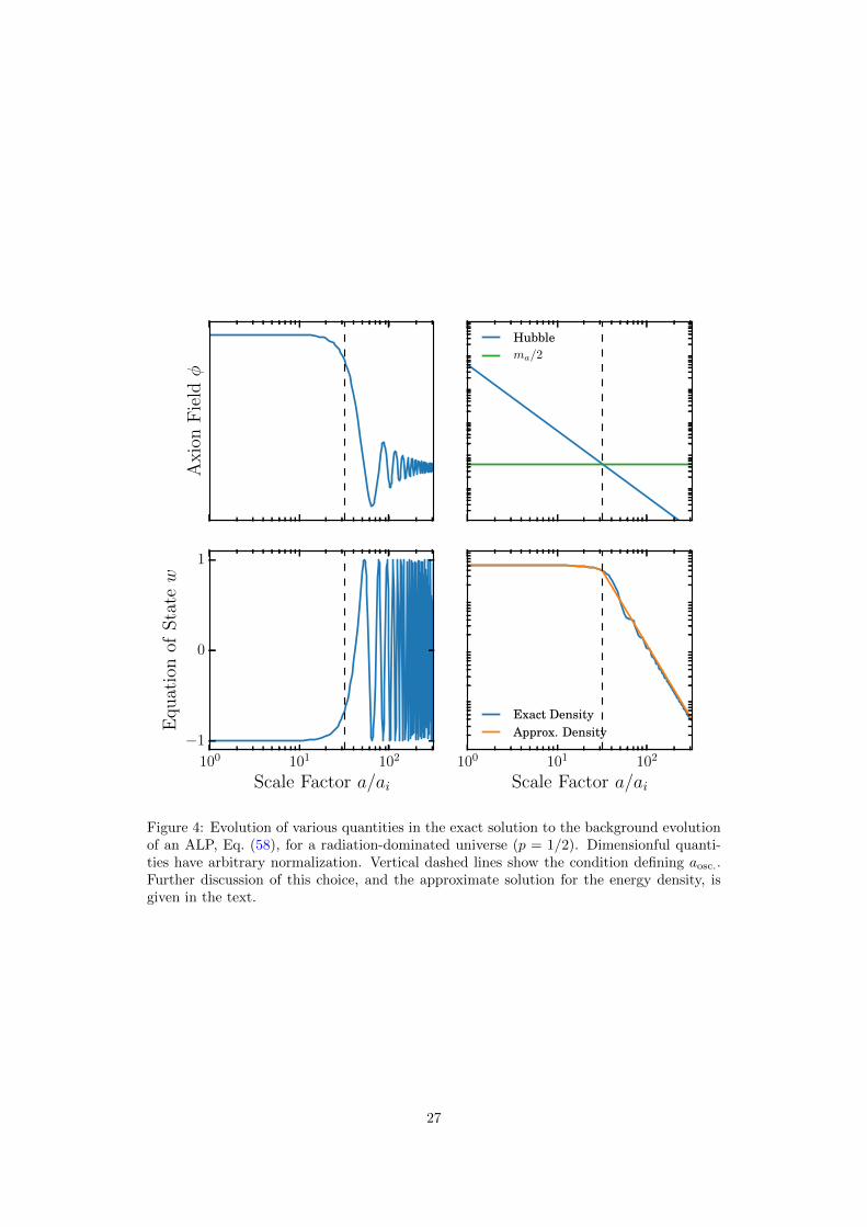
Axio

nFie

ld

Hubblema/2

100 101 102

Scale Factor a/ai

1

0

1

Equat

ion

ofSta

tew

100 101 102

Scale Factor a/ai

Exact DensityApprox. Density

Figure 4: Evolution of various quantities in the exact solution to the background evolutionof an ALP, Eq. (58), for a radiation-dominated universe (p = 1/2). Dimensionful quanti-ties have arbitrary normalization. Vertical dashed lines show the condition defining aosc..Further discussion of this choice, and the approximate solution for the energy density, isgiven in the text.

27

The transition in the axion equation of state can be approximated if we define a fixedvalue of the scale factor, aosc, and simply fix the behaviour of ρa(a) at late times to be

ρa(a) ≈ ρa(aosc)(aosc/a)3 ; (a > aosc) . (60)

Furthermore, the energy density is approximately constant up until aosc and so we can fur-ther approximate ρa(aosc) ≈ m2

aφ2i /2. This gives the usual approximation used to calculate

axion DM energy density. The energy density in the misalignment population is fixed bythe initial field displacement and the mass alone.

How shall we define aosc? Roughly, it is when ma & H, so we can let AH(aosc) = ma forsome constant A > 1. The larger we set A to be, the better the approximation (assuming wecompute ρa(aosc) from the exact solution). However, we must also play this off against theexpense of following oscillations in a numerical solution. The equation of motion, Eq. (38),suggests A = 3 is as a sensible-looking choice. In the example with a radiation dominateduniverse, I found A = 3 leads to a 40% error in the energy density at late times, with A = 2giving a better approximation.19 The approximation Eq. (60) and the location of aosc forA = 2 are also shown in Fig. 4.

In real-Universe examples with a matter-to-radiation transition and late time Λ dom-ination, we found in Ref. [131] that A = 3 works well in most cases. Using the knownsolutions in matter and radiation domination for H(t) to fix aosc in terms of other cos-mological parameters, this gives the following useful approximation to the ULA fractionalenergy density as a function of the initial displacement [132]:

Ωa ≈

16 (9Ωr)

3/4(maH0

)1/2⟨(

φiMpl

)2⟩

if aosc < aeq ,

96Ωm

⟨(φiMpl

)2⟩

if aeq < aosc . 1 ,

16

(maH0

)2⟨(

φiMpl

)2⟩

if aosc & 1 ,

, (61)

where I have used angle brackets to denote the average homogeneous value, to remind usof the consequences when the PQ symmetry is broken or unbroken during inflation.

Let’s use the WKB approximation to understand the background evolution further. TheWKB approximation for H ma consists of the ansatz solution

φ(t) = A(t) cos(mat+ ϑ) , (62)

where ϑ is an arbitrary phase, and A is slowly varying such that A/ma ∼ H/ma ∼ ε 1.Plugging this into Eq. (38) and working to leading order in ε gives the solutionA(a) ∝ a−3/2.Using this solution we find that the energy density simply scales as ρa ∝ A2 ∝ a−3, whilewa has rapid oscillations with frequency 2ma. Consequently, the average equation of stateon time scales t 1/ma is 〈wa〉t = 0. This gives a general proof as to why wa oscillatesaround zero and ρa ∝ a−3 at late times when H ma, independent of any assumptionsabout the background evolution being matter or radiation dominated.20

The solution for φ and ρa in the WKB approximation sheds light on the constant-massassumption we made at the beginning of this section. The magnitude of non-perturbativeeffects generally varies with temperature, and so the axion mass varies with cosmologicaltime, approaching an asymptotic value for T TNP. If the asymptotic value of the masshas been reached before the axion becomes relevant in the energy density and when a < aosc

19As already stated, the approximation in general improves as A gets larger. The poor performance atA = 3 is just because the energy density is falling rapidly at this point and errors are amplified. In thiscase, 3 is not a lucky number. In numerical solutions including perturbations, taking a larger A will alwaysbe better, as the improvement shown here for A = 2 applies only to the exact background solution.

20This applies to fields oscillating in a harmonic potential, V (φ) ∼ φ2. Turner [133] proved the moregeneral result for fields oscillating in an anharmonic potential, V (φ) ∼ φα, giving ρ ∝ a−6α/(α+2).

28

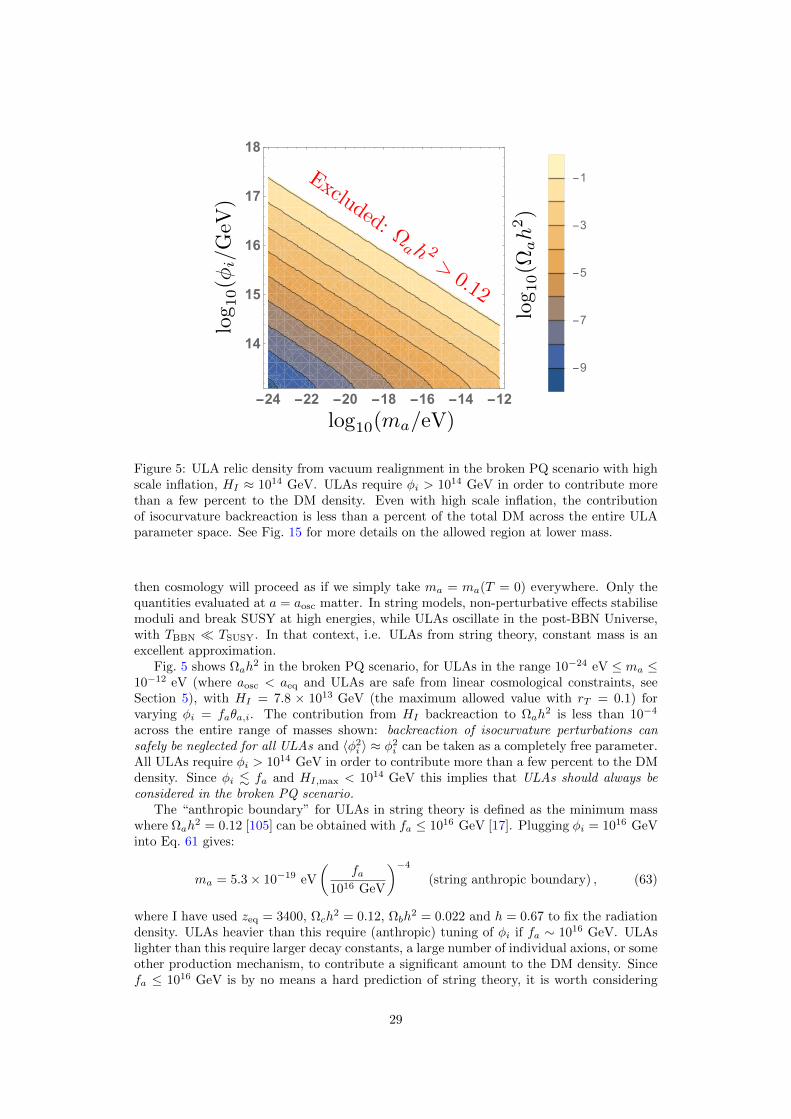
-24 -22 -20 -18 -16 -14 -12

14

15

16

17

18

Excluded: ah 2

>0.12

-9

-7

-5

-3

-1

log10(

ah

2)

log10(ma/eV)

log10(

i/G

eV)

Figure 5: ULA relic density from vacuum realignment in the broken PQ scenario with highscale inflation, HI ≈ 1014 GeV. ULAs require φi > 1014 GeV in order to contribute morethan a few percent to the DM density. Even with high scale inflation, the contributionof isocurvature backreaction is less than a percent of the total DM across the entire ULAparameter space. See Fig. 15 for more details on the allowed region at lower mass.

then cosmology will proceed as if we simply take ma = ma(T = 0) everywhere. Only thequantities evaluated at a = aosc matter. In string models, non-perturbative effects stabilisemoduli and break SUSY at high energies, while ULAs oscillate in the post-BBN Universe,with TBBN TSUSY. In that context, i.e. ULAs from string theory, constant mass is anexcellent approximation.

Fig. 5 shows Ωah2 in the broken PQ scenario, for ULAs in the range 10−24 eV ≤ ma ≤

10−12 eV (where aosc < aeq and ULAs are safe from linear cosmological constraints, seeSection 5), with HI = 7.8 × 1013 GeV (the maximum allowed value with rT = 0.1) forvarying φi = faθa,i. The contribution from HI backreaction to Ωah

2 is less than 10−4

across the entire range of masses shown: backreaction of isocurvature perturbations cansafely be neglected for all ULAs and 〈φ2

i 〉 ≈ φ2i can be taken as a completely free parameter.

All ULAs require φi > 1014 GeV in order to contribute more than a few percent to the DMdensity. Since φi . fa and HI,max < 1014 GeV this implies that ULAs should always beconsidered in the broken PQ scenario.

The “anthropic boundary” for ULAs in string theory is defined as the minimum masswhere Ωah

2 = 0.12 [105] can be obtained with fa ≤ 1016 GeV [17]. Plugging φi = 1016 GeVinto Eq. 61 gives:

ma = 5.3× 10−19 eV

(fa

1016 GeV

)−4

(string anthropic boundary) , (63)

where I have used zeq = 3400, Ωch2 = 0.12, Ωbh

2 = 0.022 and h = 0.67 to fix the radiationdensity. ULAs heavier than this require (anthropic) tuning of φi if fa ∼ 1016 GeV. ULAslighter than this require larger decay constants, a large number of individual axions, or someother production mechanism, to contribute a significant amount to the DM density. Sincefa ≤ 1016 GeV is by no means a hard prediction of string theory, it is worth considering

29

the limit of the anthropic boundary for DM-like axions with ma = 10−24 eV. This is visiblein Fig. 5, and from the fa scaling of Eq. (63). We find fa ≤ 4 × 1017 GeV: ULA DM isnatural for comfortably sub-Planckian values of the decay constant.

4.3.2 The QCD Axion

QCD non-perturbative effects switch on at T ∼ ΛQCD ∼ 200 MeV, precisely when the QCDaxion with intermediate fa begins oscillations. The temperature dependence of the axionmass in QCD is given by:

m2a(T )f2

a = χtop.(T ) , (64)

where χtop.(T ) is the QCD topological susceptibility, which must be calculated. The originalcalculation is due to Ref. [41] and is reviewed in e.g. Ref. [134], while a modern calculationin the ‘interacting instanton liquid model’ (IILM) is given in Ref. [113]. A simple power-lawdependence of the axion mass on temperature applies at high temperatures, T > 1 GeV:

m2a(T ) = αa

Λ3QCDmu

f2a

(T

ΛQCD

)−n. (65)

This should be matched to the zero temperature value, Eq. (5), at low T . ΛQCD.The standard [41] value for the power-law from the dilute instanton gas model (DIGM)

is n = 7+nf/3+· · · ≈ 8 (where nf is the number of fermions active at a given temperature).The fits of Ref. [113] from the IILM give n = 6.68 and αa = 1.68× 10−7 (which also agreeswith Ref. [135]). The temperature dependence can also be computed non-perturbativelyon the lattice in the pure Yang-Mills limit (e.g. Refs. [136, 137, 138, 139]), and at lowtemperatures from chiral perturbation theory (for a recent calculation, see Ref. [140] andreferences therein). The lattice calculations of Ref. [136] find n = 5.64 (compare to thepure Yang-Mills, nf = 0, DIGM). Ref. [140] consider a range between n = 2 and n = 8from lattice and instanton calculations respectively.

The temperature of the Universe in the radiation dominated era is determined by theFriedmann equation in the form

3H2M2pl =

π2

30g?T

4 . (66)

Taking the standard n = 8 result, using that g? = 61.75 for tempertaures just above theQCD phase transition, and defining 3H(Tosc) = ma, the QCD axion with fa < 2×1015 GeVbegins oscillating when T > 1 GeV [134]. From this point on, axion energy density scalesas a−3 independently of the behaviour of ma(T ). The relic density can thus be reliablycomputed from the high-temperature power-law behaviour of ma(T ), scaled as a−3 fromTosc. The relic density is fixed by the initial misalignment angle and fa. For fa < 2 ×1015 GeV it is given by [134]

Ωah2 ∼ 2× 104

(fa

1016 GeV

)7/6

〈θ2a,i〉 . (67)

For fa & 2× 1017 GeV oscillations begin when T < ΛQCD, such that the mass has reachedits zero-temperature value. In this case the relic density is

Ωah2 ≈ 5× 103

(fa

1016 GeV

)3/2

〈θ2a,i〉 . (68)

Note that there is not an overlapping region of validity for Eqs. (67) and (68). For2 × 1015 GeV . fa . 2 × 1017 GeV oscillations begin during the QCD epoch, the diluteinstanton gas approximation breaks down and the relic density calculation is more compli-cated (see e.g. Refs. [134, 113, 141]). However, it is argued in Ref. [134] that Eq. (67) is a

30

good approximation for fa < 6× 1017 GeV. For our simple purposes of illustration, we useEq. (67) for all fa < Mpl.

So far, we have computed the relic density using the harmonic potential, V (φ) =m2aφ

2/2. For large initial displacements, θi & 1, anharmonic corrections caused by ax-ion self-interactions become important. The potential becomes flatter at increased θPQ,causing the axion field to spend more time with wa ≈ −1, thus delaying aosc and increasingthe relic abundance relative to the harmonic approximation. Anharmonic effects can betaken into account with a correction factor by replacing

〈θ2a,i〉 → 〈θ2

a,iFanh.(θa,i)〉 , (69)

where Fanh.(x) → 1 for small x and monotonically increases as x → π. An analyticapproximation to Fanh.(x) for the cosine potential is [142]

Fanh.(x) =

[ln

(e

1− x2/π2

)]7/6

. (70)

Note that the use of Eqs. (69) and (70) breaks down if the axion field comes to dominatethe energy density, driving a period of inflation, since they rely on the assumption thatoscillations begin in a radiation-dominated background.

A full numerical computation of the relic abundance valid for all fa in the IILM, takinginto account the temperature dependence of g? in the standard model and all anharmoniceffects, is given in Ref. [113].

Axions produced by misalignment behave as DM, and we know that the DM densityis Ωch

2 ≈ 0.12. Axions may not be all the DM, but they had better not produce toomuch of it, so we must have Ωah

2 < 0.12.21 Eq. (67), and its anharmonic correctionsEqs. (69) and (70), inform the classic discussions on the QCD axion and “natural” valuesfor fa [25, 27, 26, 143].

First, let’s just take 〈θ2a,i〉 to be a free parameter, and work out the consequences. High

fa axions produce too much DM unless θa,i 1. On the other hand, low fa axions canonly produce a fraction of the DM unless θa,i is tuned very close to π such that anharmoniccorrections can boost the relic density. The “sweet spot” where Ωah

2 = 0.12 is achievedfor θa,i ≈ 1 is at fa ≈ 3 × 1011 GeV. The range of fa where Ωah

2 ≈ 0.12 can be achievedwith minimal tuning of θa,i towards zero or π is the region where broken PQ axions are“natural.” It’s boundaries clearly depend on taste, but allowing for tuning at the level 10−2

it is:8× 109 GeV . fa . 1× 1015 GeV (no tuning, broken PQ) . (71)

In the unbroken PQ scenario the relic abundance is fixed by taking 〈θ2a,i〉 = π2/3. Keeping

Ωah2 < 0.12 and satisfying bounds from stellar cooling and supernovae defines the classic

axion window :

1× 109 GeV . fa . 8.5× 1010 GeV (classic axion window, unbroken PQ) . (72)

Axions with fa & 1015 GeV are sometimes referred to as living in the anthropic axionwindow [144, 145, 146]. It is so-called because although θa,i must be tuned small, if it wasnot small and the DM density was too large, the Universe would not be conducive to theformation of galaxies and life.22 Note that the anthropic window is automatically open

21Violating this constraint is sometimes, misleadingly, called “overclosing the Universe,” a phrase whichdates from before the precision cosmology era, when one simply demanded ρa < ρcrit for some approximatevalue of H0.

22Refs. [147, 148] discuss the interesting case of anthropic selection with multiple axion fields. An addi-tional fine-tuning measure is also applied based on isocurvature perturbations (see Section 5.4). However,when applied to iscourvature, the measure used in Refs. [147, 148] assumes that the inflationary parameterεinf has a flat prior. A least information (Jeffreys) prior on the unknown physical scale HI would yield verydifferent conclusions.

31

10 12 14 16 18-5

-4

-3

-2

-1

0

-7

-5

-3

-1

log10(fa/GeV)

log10 a

,i

log10(

ah

2)

log10(fa/GeV)

log10 a

,i

log10(

ah

2)

-2

-1

14 15 16 17 18-5

-4

-3

-2

-1

0

Figure 6: QCD axion DM relic density from vacuum realignment in the broken PQ scenario.Isocurvature constraints are ignored, see Fig. 17. Left panel : Low scale inflation, HI =2π × 109 GeV. All of the allowed range of fa has PQ symmetry unbroken during inflation.Large fa requires tuning θa,i in order not to produce too much DM. Right Panel: High scaleinflation, HI = 1014 GeV. Backreaction produces too much DM for all fa . 3× 1015 GeV.

to high fa axions, since for rT < 1, fa & 1015 GeV is always in the broken PQ scenariowhere θa,i is a free parameter, although the backreaction contribution may be importantdepending on the value of HI .

Let’s bring together everything we know about the QCD axion DM relic density fromvacuum realignment into two equations:

Ωah2 ≈

2× 104(

fa1016 GeV

)7/6π2

3 Fanh.(π/√

3)(1 + αdec) (unbroken PQ) ,

2× 104(

fa1016 GeV

)7/6

(θ2a,i +H2

I /(2πfa)2)Fanh.

(√θ2a,i +H2

I /(2πfa)2)

(broken PQ) .(73)

For simplicity, as stated above, I am going to assume that Eq. (67) holds for all fa (see thediscussion below Eq. 68). See Section 3.3.2 and 4.7 for discussion on the difference betweenthe misalignment and topological defect populations.

Fig. 6 is a contour plot of Ωah2 as a function of fa and θa,i for the broken PQ scenario

in two different inflation models. The first takes HI = 2π × 109 GeV, so that all of theallowed range of fa has the PQ symmetry broken during inflation. The second scenario takesHI = 1014 GeV, i.e. about as large as it can be without violating current tensor constraints.In the case of low scale inflation, the entire allowed range of fa can produce the requiredDM density by vacuum realignment. Large fa requires tuning of θa,i in order to satisfyΩah

2 < 0.12. In the high scale inflation case, backreaction of isocurvature perturbationsleads to too much DM production for fa . 5 × 1016 GeV. Large fa & 5 × 1016 GeVanthropic axions appear compatible with high scale inflation if we allow θa,i to be tuned,however we have so far only considered constraints from the relic density, and not from theisocurvature amplitude. We will see in Section 5.4 that isocurvature constraints imply thathigh-fa axions are essentially incompatible with high-scale inflation.

Fig. 7 is a contour plot of Ωah2 as a function of fa and αdec. in the unbroken PQ

scenario. Based on constraints from rT , the largest possible value of fa in this scenario isfa ≈ 1014 GeV/2π, and I allow αdec ∈ [0.16, 186]. In the unbroken PQ scenario, the fixedvalue of 〈θ2

a,i〉 = π2/3 excludes all axions with fa & 9× 1010 GeV for producing too muchDM. The possible range of αdec values means that all axions with lower fa than this have the

32

9 10 11 12 13

-0.5

0.0

0.5

1.0

1.5

2.0

log10(fa/GeV)

log10(

ah

2)

log10↵

dec

-3

-2.5

-2

-1.5

-1

Figure 7: QCD axion DM relic density from vacuum realignment in the unbroken PQscenario. The fixed value of 〈θ2

a,i〉 = π2/3 excludes all axions with fa & 9 × 1010 GeV forproducing too much DM. The uncertainty in axion production from string decay, reflected inthe range for αdec, means that all axions with lower fa can produce a significant contributionto the DM.

possibility of providing the correct DM abundance. This defines the classic axion window.Note that if αdec & 200 then the QCD axion in the unbroken PQ scenario, satisfyingastrophysical constraints, would be completely excluded unless the excess DM abundancecould be diluted (e.g. by late-time entropy production). This possibility is the source ofthe controversy over the axion abundance by string decay discussed in Section 3.3.2.

4.4 Cosmological Perturbation Theory

All specific results here assume that cosmological history begins in the radiation dominateduniverse after reheating. I work in two gauges: the synchronous gauge and the Newtoniangauge. These gauges, the gauge transformations between them and the equations of motionfor matter and radiation, are given in the classic, and endlessly useful, Ref. [149] (see alsoRef. [150]).23 The Newtonian gauge is useful (obviously) for the Newtonian limit (discussedin more detail in the following subsection). The Newtonian potentials Ψ and Φ are alsotransparently related to the gauge invariant curvature perturbation, and to the integratedSachs-Wolfe (ISW) source terms for the CMB. The synchronous gauge, with potentials h(not to be confused with the reduced Hubble rate, also denoted h) and η, on the otherhand, makes the CDM evolution particularly simple, as θc ≡ 0. The synchronous gauge isalso used by the popular CMB Boltzmann solver camb [153]. The full treatment of ULAsin the synchronous gauge has been implemented in axionCAMB, described in Ref. [131],and soon to be publicly released. Another popular Boltzmann solver is class [154, 155],with a ULA model implemented in Ref. [156].

23As usual in cosmology, note that the adage “the Russians did it first” holds very well here. If you areso inclined, you can find everything you need in Landau and Lifschitz [151]. Another useful early referenceis Ref. [152]. I refer explicitly to Ref. [149] as it addresses specifically the CMB computation.

33

In this section I work primarily in the fluid treatment of axion perturbations. This canbe derived from the perturbed field equation. In Fourier space in synchronous gauge this is

δφ′′ + 2Hδφ′ + (k2 +m2aa

2)δφ = −1

2φ′h′ , (74)

while in Newtonian gauge it is

δφ′′ + 2Hδφ′ + (k2 +m2aa

2)δφ = (Ψ′ + 3Φ′)φ′ − 2m2aa

2φΨ , (75)

where primes denote derivatives with respect to conformal time, adτ = dt (not to beconfused with the optical depth, also denoted τ), and the conformal Hubble rate is H = aH.The perturbed axion field is δφ; the background field is φ.

4.4.1 Initial Conditions

Initial conditions are set for all modes, k, when they are super-horizon k aH and atearly times during the radiation era. I present the simplest, zeroth order initial conditions.Corrections to these results can be derived order-by-order in the super-horizon/early-timelimit. The computation is described in Ref. [157], with results specific to axions given inRef. [131].

If all cosmological perturbations are seeded by single field inflation, the initial conditionsare adiabatic. Radiation is the dominant component at early times, and carries the infla-tionary curvature perturbation. The adiabatic condition relates the overdensity in photonsto the overdensity in any other fluid component, i:

δi =3

4(1 + wi)δγ . (76)

At early times, the axion equation of state is wa ≈ −1 and so δa = δφ = 0 in the adiabaticmode in the early-time, super-horizon perturbative-expansion.

This adiabatic initial condition seems very different from the standard CDM adiabaticinitial condition where δc = 3δγ/4. That is because we are beginning when axions are notbehaving as CDM. As the axion field rolls and begins oscillating around wa = 0, the axionsbegin to cluster and fall into the potential wells set up by the photons. At late times,a > aosc, this evolution “locks on” to the standard CDM behaviour on large scales, as wewill show from numerical results shortly.

Isocurvature initial conditions can be thought of in a number of ways. Commonly, theyare thought of as entropy perturbations: i.e. perturbations in relative number density ofparticles of different species that leave the total curvature unperturbed. An isocurvatureperturbation between two species, i and j, can be written in a gauge invariant way as (e.g.Ref. [158] and references therein)

Sij = 3(ζi − ζj) (77)

where ζi is the curvature perturbation due to a single species:

ζi = −Ψ−H δρiρi

. (78)

The total curvature perturbation is

ζ =

∑i(ρi + Pi)ζi∑i(ρi + Pi)

. (79)

The most useful practical definition for all cosmological initial conditions is to think ofthem as simply the different normal (eigen) modes of the energy momentum tensor [157].One then finds the early time, τ 1, super horizon, kτ 1, expansion for each mode. In

34

the synchronous gauge each mode can be identified by the leading, zeroth order, behaviourof the fluid variables and the metric potentials:

η = 1 (adiabatic mode) , (80)

δi = 1 (density isocurvature in species i) , (81)

θi = k (velocity isocurvature in species i) , (82)

with all other components unperturbed. At higher orders one then selects the growing modefor each component. The correct selection of this is crucial. For example the adiabatic modehas (e.g. Refs. [149, 157])

δγ = −1

3(kτ)2 , (83)

and from the equations of motion one finds the condition Eq. (76) relates this to the otherspecies at each order in the perturbative-expansion, and also accounts for possible evolutionof wi (as is the case for the slowly rolling axion field at early times [131]).

In the axion iscocurvature mode, relevant for the broken PQ scenario, the initial condi-tion is δa = 1, with all other species unperturbed at zeroth order. The normalization andspectrum can be multiplied afterwards since the equations are linear. The spectrum is apower law, with spectral index (1 − nI) = 2εinf (for inflationary slow-roll parameter εinf ,see Section 7.2).

4.4.2 Early Time Treatment

At early times, the background equation of motion should be solved numerically to find theevolution of the axion equation of state, wa(τ). With this in hand, the background energydensity evolves as

ρ′a = −3Hρa(1 + wa) . (84)

The equation of state also specifies the evolution of the adiabatic background sound speed:

c2ad = wa −w′a

3H(1 + wa). (85)

The second order perturbed equations of motion can be rewritten as two first orderequations for the axion overdensity, δa and dimensionless perturbed heat flux, ua = (1 +wa)va. The equation of state and adiabatic sound speed specify the background evolution-dependent co-efficients in the equations of motion for the fluid components. Using the resultthat the sound speed in perturbations, c2s = δPa/δρa = 1 in the δφ = 0 axion comovinggauge, the transformation to fluid variables can be performed exactly [159]. Performing agauge transformation to the synchronous gauge, the equations of motion read [131]:

δ′a = −kua − (1 + wa)h′/2− 3H(1− wa)δa − 9H2(1− c2ad)ua/k , (86)

u′a = 2Hua + kδa + 3H(wa − c2ad)ua . (87)

I stress that at this stage no approximations have been made. Given the evolution of wa(τ)(or equivalently φ(τ)) the evolution of δa and ua specify the evolution of δφ (with metricpotentials sourced by all species).

Note that if φ′ = 0 then wa = −1 and w′a = 0. In this case, an adiabatic fluctuationwith δφ = δφ′ = 0 in Eq. (74) has no source and will not grow. The same holds in thefluid variables: wa = −1 leads to vanishing metric source in the fluid equations, and so ifδa = ua = 0 initially then this remains so, and no growth occurs.

In this picture, the axions source the Einstein equations with density, pressure andvelocity perturbations as

δρa = ρaδa , (88)

δPa = ρa[δa + 3H(1− c2ad)(1 + wa)ua/k] , (89)

ρa(1 + wa)va = ρaua . (90)

35

4.4.3 The Axion Effective Sound Speed

When a > aosc, wa and c2ad oscillate rapidly in time compared to the Hubble scale andall other quantities of interest (e.g. the curvature perturbation evolves on time scales oforder H). The exact fluid equations now become numerically expensive to solve, and anapproximation for the perturbed fluid equations, akin to the wa = 0 approximation in thebackground equations of motion, is necessary.

Consider the general equation of motion for fluids in synchronous gauge [149]:

δ′ = −(1 + w)(θ + h′/2)− 3H(c2s − w)δ ,

θ′ = −H(1− 3w)θ − w′

1 + wθ +

c2s1 + w

k2δ , (91)

where I have only assumed the vanishing of anisotropic stress, which is valid at first orderin perturbation theory for a scalar field. The evolution is specified by two quantites: theequation of state, w, and the sound speed in perturbations:24

c2s =δP

δρ. (92)

For an axion at late times, a > aosc, we know how to approximate the time averagedequation of state: 〈wa〉t = 〈w′a〉t = 0 (see Section 4.3.1). If we can simply find a similarexpression for 〈c2s〉t evaluated in the appropriate gauge, then we can use Eqs. (91) to specifythe evolution of the axion overdensity. The pressure source of the Einstein equations dueto axions will then be given by δPa = 〈c2s〉tρaδa.

Just as for the background, we can use the WKB approximation by writing the back-ground field and field perturbation as

φ = a−3/2[φ+ cosmt+ φ− sinmt] , (93)

δφ = δφ+ cosmt+ δφ− sinmt , (94)

where the functions δφ± depend on wavenumber k as well as time. It is now possible tofind the effective sound sound speed in the gauge comoving with the time-averaged axionfluid (see e.g. Refs. [160, 161] for the derivation):

〈c2s〉t = c2s,eff =k2/4m2

aa2

1 + k2/4m2aa

2. (95)

This effective sound speed is the key to understanding the difference between ULAs andCDM in terms of structure formation.

The metric potentials in the axion comoving gauge are defined in the same way as thesynchronous gauge. The gauge transformation between the two gauges induces additionalterms to Eqs. (91) that decay on sub-horizon scales [131]. The axion fluid equations ofmotion in the synchronous gauge are:

δ′a = −kua −h′

2− 3Hc2s,effδa − 9H2c2s,effua/k, (96)

u′a = −Hua + c2s,effkδa + 3c2s,effH2ua. (97)

4.4.4 Growth of Perturbations and the Axion Jeans Scale

So far, we’ve been very precise and set up the equations of motion and initial conditionsas they would be used in numerical Boltzmann equation solver to compute cosmologicalobservables in the real Universe.

24See Appendix D for discussion of different definitions of the scalar field sound speed and the relationsbetween them.

36

100 101 102

ScaleFactor a/ai

10−6

10−5

10−4

10−3

10−2

10−1

100

101

102

103

Ove

rden

sity

low k

medium k

high k

100 101 102

ScaleFactor a/ai

10−7

10−6

10−5

10−4

10−3

10−2

10−1

100

101

Ove

rden

sity

low k

medium k

high k

Figure 8: The exact scale-dependent linear growth for an axion DM dominated universe,Eq. (102), at three values of k = k/

√maH0, as a function of a/ai. Normalization is

arbitrary. Note that the initial scale factor in this case must obey ai > aosc for the solutionsto hold. Left panel : The growing mode, D+(k, a), Eq. (103). Right Panel: The decayingmode, D−(k, a), Eq. (104).

Let’s take a step back for a moment to a simplified situation, and consider a Universedominated by axion DM, and work in the Newtonian gauge. Let’s take the sub-horizonlimit, so that we can use the Poisson equation in its usual form:

k2Ψ2 = −4πGa2ρδ (98)

Gauge transformations on the effective sound speed between the synchronous and Newto-nian gauge also vanish in this limit. Combining the equations for δa and θa into a singlesecond order equation for δa, and using the Poisson equation to eliminate the Netwonianpotential, gives the equation of motion for δa in physical time:

δa + 2Hδa + (k2c2s,eff/a2 − 4πGρa)δa = 0 . (99)

This is the equation for an oscillator with time-dependent mass and friction. The mass termin this equation expresses the competition between density and pressure during gravitationalcollapse. The origin of the effective sound speed and pressure in the axion equation of motionis scalar field gradient energy.

On large scales, k2c2s → 0, density wins and axion DM has a Jeans instability [162].25

The equation of motion is exactly the same as for CDM, with the usual growing, δa ∝ a,and decaying, δa ∝ a−3/2, modes. On small scales, the pressure term dominates over thedensity, and δa oscillates without growing.

The scale where density and pressure are in equilibrium and 4πGρa = k2c2s is known asa the axion Jeans scale, and it defines a particular wavenumber, kJ . Modes with k < kJgrow, while modes with k > kJ oscillate. The buzz-phrase to remember referring to axionperturbations is that there is scale-dependent growth, and that axion DM differs from CDMon scales below the axion Jeans scale.

In the limit k/maa < 1 the sound speed has the approximate form:

c2s,eff ≈k2

4m2aa

2. (100)

25The growth of perturbations for small k, despite positive mass-squared for the perturbations in Eqs. (74)and (75), can be understood from the rapid oscillations in φ′ causing the system to act as a driven oscilla-tor [159, 163].

37

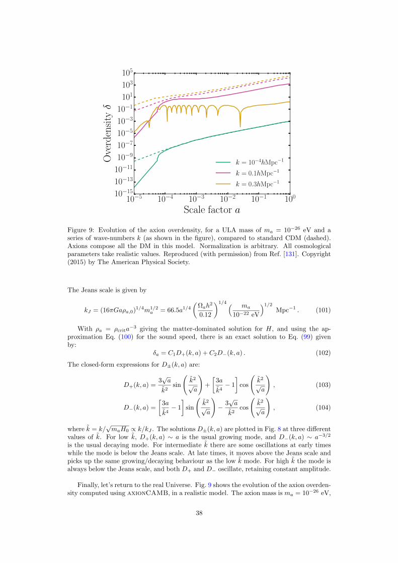
10−5 10−4 10−3 10−2 10−1 100

Scale factor a

10−15

10−13

10−11

10−9

10−7

10−5

10−3

10−1

101

103

105

Ove

rden

sityδ

k = 10−4hMpc−1

k = 0.1hMpc−1

k = 0.3hMpc−1

Figure 9: Evolution of the axion overdensity, for a ULA mass of ma = 10−26 eV and aseries of wave-numbers k (as shown in the figure), compared to standard CDM (dashed).Axions compose all the DM in this model. Normalization is arbitrary. All cosmologicalparameters take realistic values. Reproduced (with permission) from Ref. [131]. Copyright(2015) by The American Physical Society.

The Jeans scale is given by

kJ = (16πGaρa,0)1/4m1/2a = 66.5a1/4

(Ωah

2

0.12

)1/4 ( ma

10−22 eV

)1/2

Mpc−1 . (101)

With ρa = ρcrita−3 giving the matter-dominated solution for H, and using the ap-

proximation Eq. (100) for the sound speed, there is an exact solution to Eq. (99) givenby:

δa = C1D+(k, a) + C2D−(k, a) . (102)

The closed-form expressions for D±(k, a) are:

D+(k, a) =3√a

k2sin

(k2

√a

)+

[3a

k4− 1

]cos

(k2

√a

), (103)

D−(k, a) =

[3a

k4− 1

]sin

(k2

√a

)− 3√a

k2cos

(k2

√a

), (104)

where k = k/√maH0 ∝ k/kJ . The solutions D±(k, a) are plotted in Fig. 8 at three different

values of k. For low k, D+(k, a) ∼ a is the usual growing mode, and D−(k, a) ∼ a−3/2

is the usual decaying mode. For intermediate k there are some oscillations at early timeswhile the mode is below the Jeans scale. At late times, it moves above the Jeans scale andpicks up the same growing/decaying behaviour as the low k mode. For high k the mode isalways below the Jeans scale, and both D+ and D− oscillate, retaining constant amplitude.

Finally, let’s return to the real Universe. Fig. 9 shows the evolution of the axion overden-sity computed using axionCAMB, in a realistic model. The axion mass is ma = 10−26 eV,

38

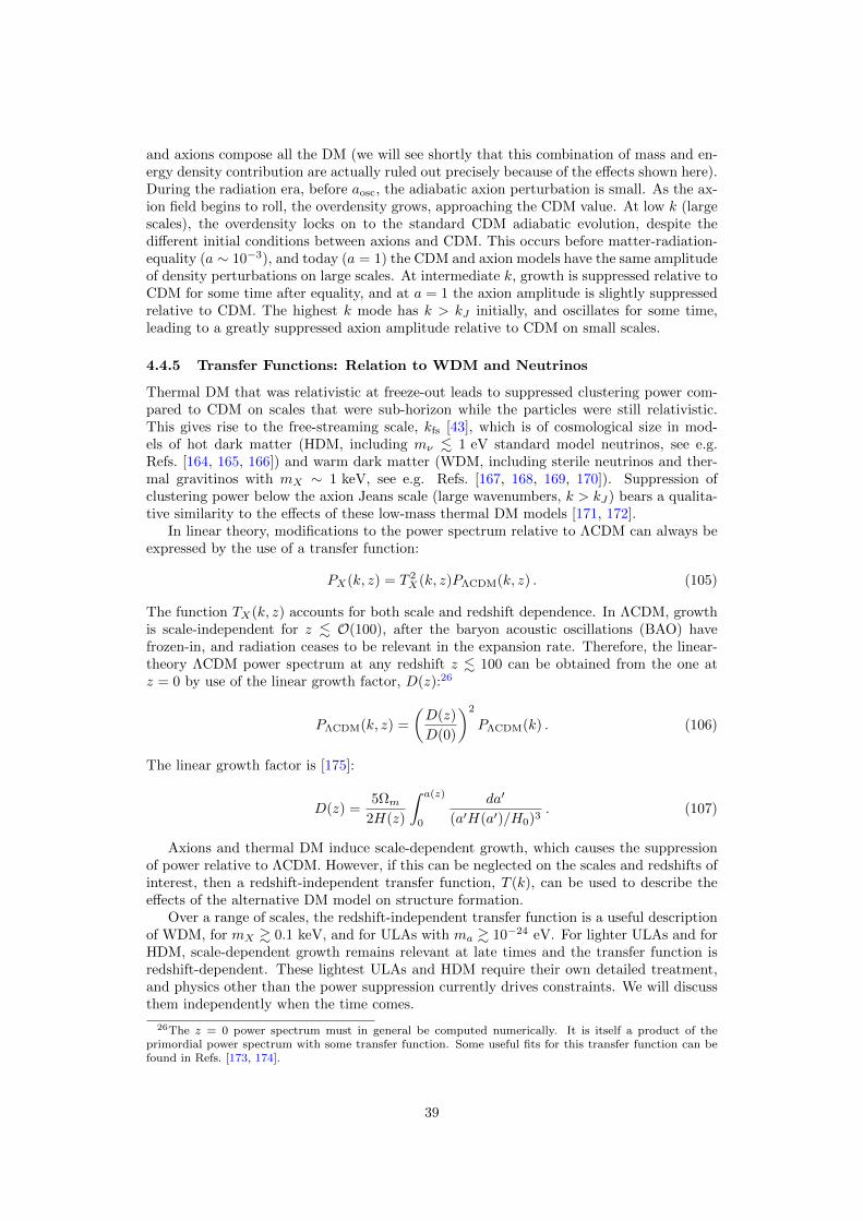
and axions compose all the DM (we will see shortly that this combination of mass and en-ergy density contribution are actually ruled out precisely because of the effects shown here).During the radiation era, before aosc, the adiabatic axion perturbation is small. As the ax-ion field begins to roll, the overdensity grows, approaching the CDM value. At low k (largescales), the overdensity locks on to the standard CDM adiabatic evolution, despite thedifferent initial conditions between axions and CDM. This occurs before matter-radiation-equality (a ∼ 10−3), and today (a = 1) the CDM and axion models have the same amplitudeof density perturbations on large scales. At intermediate k, growth is suppressed relative toCDM for some time after equality, and at a = 1 the axion amplitude is slightly suppressedrelative to CDM. The highest k mode has k > kJ initially, and oscillates for some time,leading to a greatly suppressed axion amplitude relative to CDM on small scales.

4.4.5 Transfer Functions: Relation to WDM and Neutrinos

Thermal DM that was relativistic at freeze-out leads to suppressed clustering power com-pared to CDM on scales that were sub-horizon while the particles were still relativistic.This gives rise to the free-streaming scale, kfs [43], which is of cosmological size in mod-els of hot dark matter (HDM, including mν . 1 eV standard model neutrinos, see e.g.Refs. [164, 165, 166]) and warm dark matter (WDM, including sterile neutrinos and ther-mal gravitinos with mX ∼ 1 keV, see e.g. Refs. [167, 168, 169, 170]). Suppression ofclustering power below the axion Jeans scale (large wavenumbers, k > kJ) bears a qualita-tive similarity to the effects of these low-mass thermal DM models [171, 172].

In linear theory, modifications to the power spectrum relative to ΛCDM can always beexpressed by the use of a transfer function:

PX(k, z) = T 2X(k, z)PΛCDM(k, z) . (105)

The function TX(k, z) accounts for both scale and redshift dependence. In ΛCDM, growthis scale-independent for z . O(100), after the baryon acoustic oscillations (BAO) havefrozen-in, and radiation ceases to be relevant in the expansion rate. Therefore, the linear-theory ΛCDM power spectrum at any redshift z . 100 can be obtained from the one atz = 0 by use of the linear growth factor, D(z):26

PΛCDM(k, z) =

(D(z)

D(0)

)2

PΛCDM(k) . (106)

The linear growth factor is [175]:

D(z) =5Ωm

2H(z)

∫ a(z)

0

da′

(a′H(a′)/H0)3. (107)

Axions and thermal DM induce scale-dependent growth, which causes the suppressionof power relative to ΛCDM. However, if this can be neglected on the scales and redshifts ofinterest, then a redshift-independent transfer function, T (k), can be used to describe theeffects of the alternative DM model on structure formation.

Over a range of scales, the redshift-independent transfer function is a useful descriptionof WDM, for mX & 0.1 keV, and for ULAs with ma & 10−24 eV. For lighter ULAs and forHDM, scale-dependent growth remains relevant at late times and the transfer function isredshift-dependent. These lightest ULAs and HDM require their own detailed treatment,and physics other than the power suppression currently drives constraints. We will discussthem independently when the time comes.

26The z = 0 power spectrum must in general be computed numerically. It is itself a product of theprimordial power spectrum with some transfer function. Some useful fits for this transfer function can befound in Refs. [173, 174].

39

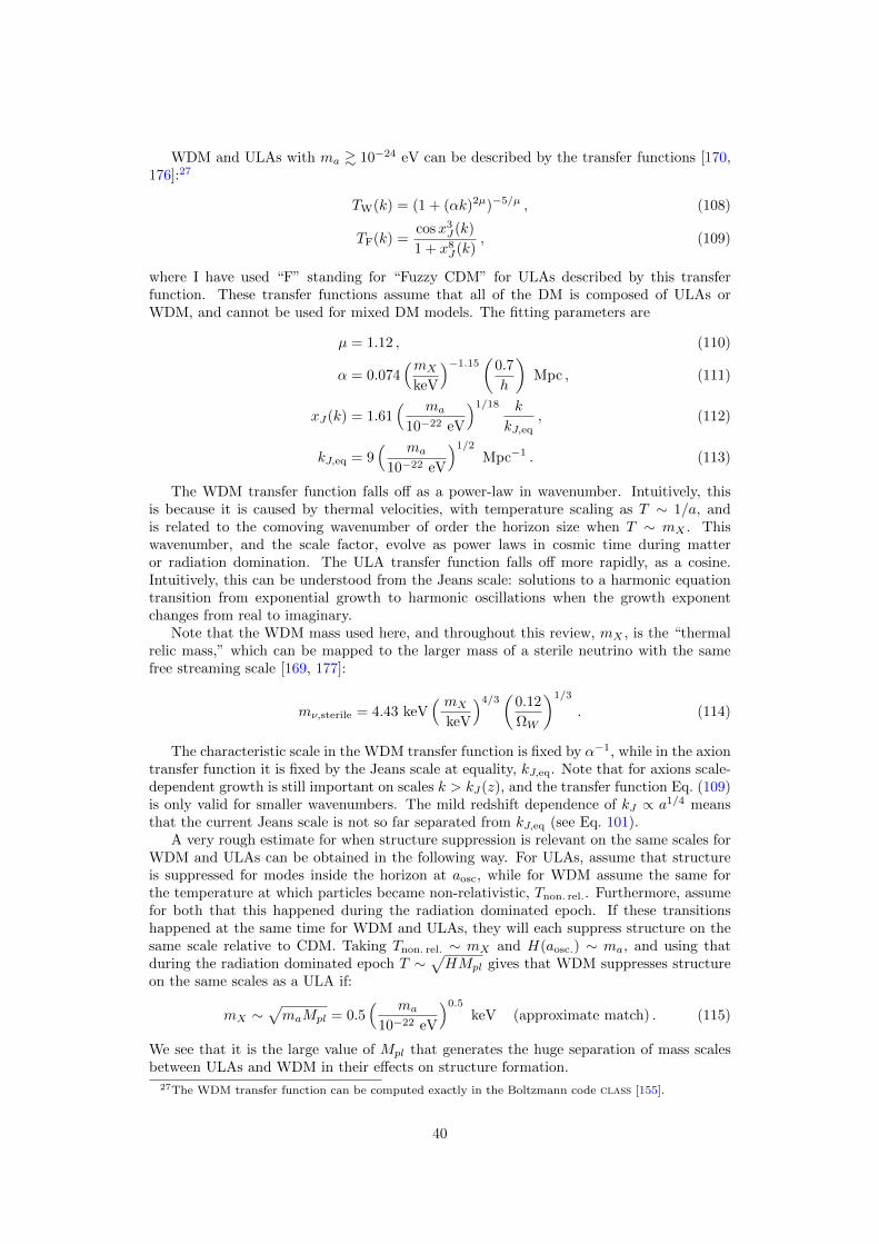
WDM and ULAs with ma & 10−24 eV can be described by the transfer functions [170,176]:27

TW(k) = (1 + (αk)2µ)−5/µ , (108)

TF(k) =cosx3

J(k)

1 + x8J(k)

, (109)

where I have used “F” standing for “Fuzzy CDM” for ULAs described by this transferfunction. These transfer functions assume that all of the DM is composed of ULAs orWDM, and cannot be used for mixed DM models. The fitting parameters are

µ = 1.12 , (110)

α = 0.074(mX

keV

)−1.15(

0.7

h

)Mpc , (111)

xJ(k) = 1.61( ma

10−22 eV

)1/18 k

kJ,eq, (112)

kJ,eq = 9( ma

10−22 eV

)1/2

Mpc−1 . (113)

The WDM transfer function falls off as a power-law in wavenumber. Intuitively, thisis because it is caused by thermal velocities, with temperature scaling as T ∼ 1/a, andis related to the comoving wavenumber of order the horizon size when T ∼ mX . Thiswavenumber, and the scale factor, evolve as power laws in cosmic time during matteror radiation domination. The ULA transfer function falls off more rapidly, as a cosine.Intuitively, this can be understood from the Jeans scale: solutions to a harmonic equationtransition from exponential growth to harmonic oscillations when the growth exponentchanges from real to imaginary.

Note that the WDM mass used here, and throughout this review, mX , is the “thermalrelic mass,” which can be mapped to the larger mass of a sterile neutrino with the samefree streaming scale [169, 177]:

mν,sterile = 4.43 keV( mX

keV

)4/3(

0.12

ΩW

)1/3

. (114)

The characteristic scale in the WDM transfer function is fixed by α−1, while in the axiontransfer function it is fixed by the Jeans scale at equality, kJ,eq. Note that for axions scale-dependent growth is still important on scales k > kJ(z), and the transfer function Eq. (109)is only valid for smaller wavenumbers. The mild redshift dependence of kJ ∝ a1/4 meansthat the current Jeans scale is not so far separated from kJ,eq (see Eq. 101).

A very rough estimate for when structure suppression is relevant on the same scales forWDM and ULAs can be obtained in the following way. For ULAs, assume that structureis suppressed for modes inside the horizon at aosc, while for WDM assume the same forthe temperature at which particles became non-relativistic, Tnon. rel.. Furthermore, assumefor both that this happened during the radiation dominated epoch. If these transitionshappened at the same time for WDM and ULAs, they will each suppress structure on thesame scale relative to CDM. Taking Tnon. rel. ∼ mX and H(aosc.) ∼ ma, and using thatduring the radiation dominated epoch T ∼

√HMpl gives that WDM suppresses structure

on the same scales as a ULA if:

mX ∼√maMpl = 0.5

( ma

10−22 eV

)0.5

keV (approximate match) . (115)

We see that it is the large value of Mpl that generates the huge separation of mass scalesbetween ULAs and WDM in their effects on structure formation.

27The WDM transfer function can be computed exactly in the Boltzmann code class [155].

40

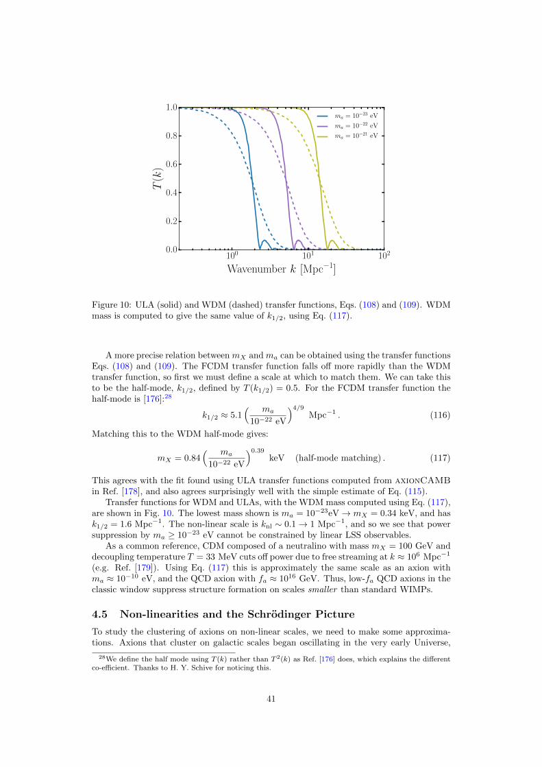
100 101 102

Wavenumber k [Mpc−1]

0.0

0.2

0.4

0.6

0.8

1.0

T(k

)

ma = 10−23 eV

ma = 10−22 eV

ma = 10−21 eV

Figure 10: ULA (solid) and WDM (dashed) transfer functions, Eqs. (108) and (109). WDMmass is computed to give the same value of k1/2, using Eq. (117).

A more precise relation between mX and ma can be obtained using the transfer functionsEqs. (108) and (109). The FCDM transfer function falls off more rapidly than the WDMtransfer function, so first we must define a scale at which to match them. We can take thisto be the half-mode, k1/2, defined by T (k1/2) = 0.5. For the FCDM transfer function thehalf-mode is [176]:28

k1/2 ≈ 5.1( ma

10−22 eV

)4/9

Mpc−1 . (116)

Matching this to the WDM half-mode gives:

mX = 0.84( ma

10−22 eV

)0.39

keV (half-mode matching) . (117)

This agrees with the fit found using ULA transfer functions computed from axionCAMBin Ref. [178], and also agrees surprisingly well with the simple estimate of Eq. (115).

Transfer functions for WDM and ULAs, with the WDM mass computed using Eq. (117),are shown in Fig. 10. The lowest mass shown is ma = 10−23eV→ mX = 0.34 keV, and hask1/2 = 1.6 Mpc−1. The non-linear scale is knl ∼ 0.1→ 1 Mpc−1, and so we see that powersuppression by ma ≥ 10−23 eV cannot be constrained by linear LSS observables.

As a common reference, CDM composed of a neutralino with mass mX = 100 GeV anddecoupling temperature T = 33 MeV cuts off power due to free streaming at k ≈ 106 Mpc−1

(e.g. Ref. [179]). Using Eq. (117) this is approximately the same scale as an axion withma ≈ 10−10 eV, and the QCD axion with fa ≈ 1016 GeV. Thus, low-fa QCD axions in theclassic window suppress structure formation on scales smaller than standard WIMPs.

4.5 Non-linearities and the Schrodinger Picture

To study the clustering of axions on non-linear scales, we need to make some approxima-tions. Axions that cluster on galactic scales began oscillating in the very early Universe,

28We define the half mode using T (k) rather than T 2(k) as Ref. [176] does, which explains the differentco-efficient. Thanks to H. Y. Schive for noticing this.

41

with aosc 1, so we can take the WKB approximation. The virial velocity in a typicalgalaxy is vvir ∼ 100 km s−1 c, and galaxies are much smaller than the horizon, so wecan take the non-relativistic approximation. Overdensities in galaxies are δ & O(105), soperturbation theory on δa or φ is no good. However, except in the vicinity of black holes,the Newtonian potential is small, Ψ 1. Thus the Newtonian limit is appropriate, andΨ obeys the Poisson equation. We will also only be concerned with scales above the axionCompton wavelength (which is on relativistic scales in the Klein-Gordon equation).

To leading order in Ψ the D’Alembertian is

= −(1− 2Ψ)(∂2t + 3H∂t) + a−2(1 + 2Ψ)∇2 − 4Ψ∂t , (118)

and the axion energy density is

ρa =1

2[(1− 2Ψ)φ2 +m2

aφ2 + a−2(1 + 2Ψ)∂iφ∂iφ] . (119)

We take the WKB approximation in the form

φ = (ma

√2)−1(ψe−imat + ψ∗eimat) , (120)

where ψ is a complex field, which can be written in polar co-ordinates as

ψ = ReiS . (121)

We take our limits as Ψ ∼ ε2NR, and k/ma ∼ εNR and H/ma ∼ εWKB, and work toquadratic order in ε ∼ εNR ∼ εWKB. In this limit, the energy density contains the leadingorder piece:

ρa = |ψ|2 = R2 , (122)

and the equation of motion for ψ is the Schrodinger equation:

iψ − 3iHψ/2 + (2maa2)−1∇2ψ −maΨψ = 0 . (123)

This is a non-linear Schrodinger equation, with Ψ sourced by |ψ|2 via the Poisson equation.The form shown here, including the Hubble friction explicitly, can be found from the usualform by going to comoving coordinates.

While the Schrodinger equation is interesting and can provide insight into structure for-mation with axion DM, wave equations don’t fit the bill as standard cosmologist’s tools. Wecan make contact with standard perturbation theory [180] and non-linear simulation toolssuch as smoothed-particle hydrodynamics (SPH) using, as before, a fluid description. Sub-stituting the polar form of the wavefunction, we can find conservation and Euler equationsfor an effective fluid described by ψ. The fluid velocity is

~va ≡ (maa)−1∇S . (124)

We can now perform a background-fluctuation split and find the equations of motion interms of the overdensity, δa (e.g. Refs. [181, 182]):

δa + a−1~va · ∇δa = −a−1(1 + δa)∇ · ~va , (125)

~va + a−1 (~va · ∇)~va = −a−1∇(Ψ +Q)−H~v , (126)

Q ≡ − 1

2m2aa

2

∇2√

1 + δa√1 + δa

, (127)

where I have defined the “quantum potential” Q.29 The quantum potential is all we needto model the axion gradient energy and Jeans scale in the full non-linear dynamics as a

29We have used the Schrodinger equation as an intermediate step to get a fluid form for the axionequations without needing to perform the background-fluctuation split on φ first. We were thus able toretain canonical equations of motion for ρ and ~v beyond linear perturbation theory. For discussion on theuse of hydrodynamics to describe quantum mechanics in the “synthetic” view of Bohmian mechanics, seeRef. [183].

42

simple modification to the force on a fluid element [182, 184]:

F = −a−1∇(Ψ +Q) . (128)

Eqs. (125) and (126) can also be used as the basis for a modified perturbation theory ofaxion DM, which takes into account the differences to CDM near the Jeans scale. ExpandingEq. (127) to first order in δa and going to Fourier space provides a simple derivation of theasymptotic form of the effective sound speed, Eq. (100).

The Schrodinger form of the field equations is useful and interesting in and of itself. Itis a fundamental (though approximate) equation governing axion DM on non-linear scales.We will use the Schrodinger equation to discuss axion halo density profiles in Section 6.3.Above the de-Broglie wavelength Schrodinger equation also accurately models CDM, and isan alternative to standard N-body simulation techniques [185]. The wave properties belowthe de Broglie scale and the introduction of the quantum force in the fluid equations are aparticular regularization and softening of the Vlasov equation [186]. They also provide asetting to study modifications to the Zel’dovich approximation [187, 181], which is the basisof Lagrangian perturbation theory. Perhaps most importantly, however, the Schrodingerequation provides the best method currently available to accurately simulate axion andscalar field DM on small scales, which we will now discuss.

4.6 Simulating axion DM

A full description of DM clustering in any model can only truly be provided by non-pertrubative numerical simulations. Since the earliest days of computational cosmology,this been studied in N -body simulations, which simulate the dynamics of collisionless pointparticles interacting via Newton’s gravitational law. The “particles” are not fundamentalparticles, but simulations particles, the mass of which is fixed by the simulations resolution.Newton’s law is “softened” on small scales to prevent unphysical two-body pairs of theseparticles dominating the dynamics. These classicN -body simulations are the perfect pictureof CDM, and their conceptual simplicity provides some explanation for the popularity ofits study.

A simulation of CDM is defined by two properties: initial conditions, and dynamics. Theinitial conditions are provided by the matter power spectrum from linear theory, with higherorder effects to deal with transients [180]; the dynamics is that of collisionless particles.Axions, particularly ULAs, modify both of these properties:

• Modified initial conditions: The initial power spectrum is suppressed relative to CDM.Modes below the Jeans scale at matter-radiation equality have the power erased.

• Modified dynamics: On scales of order the axion de Broglie wavelength, wavelikeeffects must be included. The dynamics is not that of collisionless point particles.

Modified initial conditions are easily implemented in an N -body simulation, as long asthe correct power spectrum is provided from a Boltzmann code. Such simulations providean accurate description of axions above the de Broglie wavelength, and have been performedin Refs. [188, 189]. These simulations are very similar to those of WDM in the case thatstreaming velocities are irrelevant (e.g. Refs. [170, 190]). Special care must be taken,however, due to the appearance of “spurious structures” caused by discreteness effects [191].Such spurious structures can be removed based on the shape of the protohalos [190] or onthe functional shape of the halo mass function [192]. Removal of spurious structure forULAs was carried out using the protohalo shape condition in Ref. [188]. We will discussthe halo mass function in more detail in Section 6.1.

Modified dynamics are somewhat less trivial to implement, in particular those relevantto ULAs. Modern simulations add new dynamics to the simplest CDM model such ashydrodynamics of the baryons (e.g. Ref. [193]), parameterised force law modifications for

43

variants of SIDM [194], neutrino models with streaming velocities [195, 196], and evengeneral relativistic effects [197] or modified gravity [198]. At their core, all these methodsare based, to some degree, on the N -body paradigm.

As long as the objects to be simulated are non-relativistic (as galactic halos are), theSchrodinger equation provides the correct model of axion DM on small scales. A cosmo-logical simulation of the Schrodinger equation is a fundamental departure from N -bodysimulations. The first high-resolution cosmological simulations of the Schrodinger formwere recently performed in Ref. [199]. The modified dynamics caused by wavelike effectsfor ma ≈ 10−22 eV appear in dwarf galaxy-sized objects on scales of order 1 kpc. Themodified dynamics can be seen to introduce effects including smooth halo density profilesand interference fringes (see Section 6.3 and Fig. 20), which would be completely absentin a CDM-like N -body simulation. Resolving these features accurately in a cosmologicalsimulation involves many computational technicalities, including e.g. the use of adaptivemesh refinement to solve the scalar field equation over a wide range of length scales.

An alternative way to model the modified dynamics of ULAs and other scalar fields incosmological simulations, which fits more easily into the N -body paradigm, is suggestedby the modified force law in the fluid description, Eq. 128. This modified force law couldbe implemented in a hydrodynamic model (as suggested in Refs [182, 184]), or indeed inany method where the local density and its derivatives can be accurately determined. Thismethod was employed in toy models in Ref. [184], but has yet to be applied to a cosmologicalsimulation.

The Schrodinger equation in this context models more than just axions. It is applicableto any model of scalar field DM, real or complex-valued, so long as the field is oscillatingabout a quadratic potential minimum, and self-interactions can be neglected. The simu-lations of Ref. [199] represent the state-of-the-art for simulations of these models. Thereis still much to be done in this area, however. For example, some of the many things notcovered in Ref. [199]:

• Initial conditions. Use of full Boltzmann equation power spectra. Modified perturba-tion theory and Zel’dovich approximation.

• Hydrodynamics. Modelling of baryonic effects in tandem with scalar field dynamicsto assess complementary roles.

• Zoom-in simulations. Dwarf galaxies and sub-structure modelled in Milky-Way andLocal Group analogs from larger N -body simulations.

This shopping list is not meant to detract from the achievements of Ref. [199]: the field ofstudy of such simulations is simply young compared to that of CDM N -body simulations.

4.7 My Two Cents on BEC

In this section we discuss only DM axions. There is some debate in the literature as towhether axion DM forms a Bose-Einstein condensate (BEC), and over what scales such aBEC differs from CDM. For more discussion on this topic, see Refs. [200, 201, 202, 203].The original discussions of the link between quantum theory and classical fields for theaxion are in Refs. [204, 205].30

Davidson [202] defines a BEC as

BEC = condensed regime = classical field . (129)

30There is a vast literature on so-called “BEC dark matter”: as far as I can tell, for all practical purposesthis simply maps to general scalar field models. Since the early Universe physics is often less well definedthan in the case of axions, questions of condensate formation are also less clear. For a good source ofreferences and history, see Ref. [206].

44

This chimes with our usual notion form undergraduate statistical mechanics: the macroscopically-occupied ground-state obeys the classical equations of motion. The important character-istic, however, is not the ground-state, which is only accessible to a homogeneous system(which cosmology certainly is not), but it is that the Fourier modes are concentrated at aparticular value and that the particles in this state are coherent.

Let’s define some of these notions: we will not use these formal definitions, but it helpsto be precise. QFT decomposes a field operator into modes of creation, a, and annihilation,a†, operators as

φ(x) =

∫d3p

(2π)3

1√2Ep

(ape−~p·~x + a†pe

−i~p·~x) , (130)

where ~p is the three-momentum, and Ep is the energy. The ground state is defined byap|0〉 = 0. The classical field is defined by the coherent state [207]

|φ〉 =1

Nexp

[∫d3q

(2π)3φ(~q)a†q

]|0〉 , (131)

where φ(~q) is the Fourier transform of the classical field, and N is a normalisation such that〈φ|φ〉 = 1. The expectation value of the field operator in this state is the classical field:

〈φ|φ(x)|φ〉 =

∫d3p

(2π)3

1√2Ep

φ(~p)e−i~p·~x = φ(x) , (132)

i.e. this expectation value obeys the classical equations of motion as we have been discussingin the preceding subsections, and will continue to discuss throughout this review.

The questions now are: over what timescales do axions enter the state |φ〉, how doesthis state evolve, and, crucially, what is its coherence length? The “controversy” of axionBEC is over what role gravity plays in this process, particularly at late times, and over thecoherence length this induces for structures with vorticity, ~∇× ~v 6= 0, within galaxies.

Recall that there are two populations of DM axions: those formed from vacuum re-alignment, and those formed from decay of topological defects. The vacuum realignmentpopulation begins life already in the state |φ〉. In the broken PQ scenario, the state |φ〉is formed by inflation, which super-cools and homgenises the axion field over the entirevisible Universe. In the unbroken PQ scenario, the parent PQ field, ϕ, is in it is classicalfield state, |ϕ〉, and thus the axion field created after SSB is also coherent in the state |φ〉over the horizon size at SSB (leading to the classical field configurations of strings, domainwalls, and miniclusters, as discussed above).

Thus, for either the broken or unbroken PQ scenario, axions from the vacuum realign-ment mechanism are described entirely by the classical field equations, as presented in thepreceding parts of this section. Thermalisation at early times is irrelevant, as coherence isestablished by initial conditions. The gravitational interactions lead to the usual structureformation on large scales: as perturbations grow, the field effectively loses some coherence.The Jeans scale supports the field against gravitational collapse and maintains total coher-ence on smaller scales. The characteristic size of collapsed objects is given by the solitonsolutions to the Schroodinger-Possion equation (see Section 6.3).

For the population of cold axion particles produced by topological defect decay in theunbroken PQ scenario, axions can enter the state |φ〉 via thermalisation. The condition forthermalisation due to any interactions is that the relaxation rate, Γ, is of order the Hubblerate.

Consider the QCD axion for concreteness. The self interactions are computed by Taylorexpanding the cosine potential, giving:

Vint =λ

4!φ4 , λ =

m2a

f2a

m3d +m3

u

(md +mu)3≈ 0.35

m2a

f2a

. (133)

45

Note that these interactions are attractive. The relaxation rate is [200]

Γλ ∼ nσ0δvN . (134)

where n is the number density of particles, σ0 is the cross section for two-to-two axionscattering in vacuum, σ0 = λ2/(64πm2

a), δv is the velocity dispersion, and N is the averagestate occupation number. The number density is computed from the relic density, thevelocity dispersion at time t is computed by redshifting the initial momentum, p(tosc) ≈H(tosc) (recall that topological defects decay when the classical field begins oscillating),and the occupation number is given by

N =(2π)3n

Vcoh., (135)

where Vcoh. is the spherical volume of a coherence patch: Vcoh. = 4π(mδv)3/3.By taking matosc ∼ 1 we find that Γλ(tosc)/H(tosc) ∼ O(1): self interactions thermalise

the cold population of axions, with an initial coherence length of order 1/H(tosc).31 Thus,for the cold population of axions produced by topological defect decay, on all times laterthat tosc we can also describe the axions as being in the state |φ〉 obeying the classicalequations of motion. This is as we expect: occupation numbers for axion DM from anyproduction mechanism are so huge that classical field equations ought to be adequate. Sofar, so uncontroversial.

The question now arises as to whether axions can “re-thermalise” at later times. Thetwo-to-two rate, Γλ, redshifts faster than H, such that at times after tosc self-interactionsare not sufficient for this purpose [200]. Now the controversial part: can gravitationalinteractions re-thermalise the axion condensate? If re-thermalisation at times t > tosc

occurs, then a larger coherence length will be established, and axion DM will differ fromCDM on scales larger than those set by the Jeans scale and quantum pressure in the classicalequations of motion.

Sikivie and Yang [200] propose that gravitational scattering of axions can lead to re-thermalisation of the QCD axion at a temperature Tre. ∼ 100 eV(fa/1012 GeV)1/2. Thisis argued based on the gravitational relaxation rate:

ΓG =GNnm

2a

(mδv)2. (136)

If Sikivie and Yang are correct, this effect will induce a larger coherence length for theaxion field, absent in the classical equations of motion. In particular, the claim is thatre-thermalization due to ΓG is not captured by the classical equations of motion.

However, this claim has been countered by Davidson and Elmer [201], Davidson [202],and Guth, Hertzberg and Prescod-Weinstein [203], who show that the effects of the relax-ation rate ΓG are already present in the classical equations of motion (the relevant casebeing the Schrodinger-Poisson equation), and thus by solving them alone on times t > tosc

we miss nothing: there is no coherence on scales larger than the Jeans scale. The rate ΓGis the interaction rate between axions already in the condensate with one another, hencebeing linear in GN . Davidson [202] also estimated the quadratic in GN scattering betweencold axion particles and the condensate, concluding that this interaction is negligible forfa . Mpl.

32 In the end, Davidson notes, all such questions can ultimately be answeredby the Path Integral, using the Closed Time Path 2PI action in curved space. Furthertreatment of this is far beyond the scope of this review.

A final note here is on the possible formation of vortices in the axion field (a well-knownphenomenon in BEC in the laboratory [208]), and their possible phenomenological role ingalactic haloes. A net overall rotation of the axion field caused by tidal torques leading

31The general scalings of these arguments hold also for generic ALPs with λ ∼ m2a/f

2a .

32Recall that it is folk-wisdom that super-Planckian fa violates “gravity as the weakest force”

46

to ∇× ~v 6= 0 would augment our system of classical equations due to anomalous stresses,and could lead to vortex formation. Sikivie and Yang (see also Ref. [209]) argued that thiscould be a distinctive feature of axion DM, and may explain the structure of caustics in DMhaloes. This was explored in more detail by Rindler-Daller and Shapiro [210], who foundthat the axion self-interactions are of the wrong type (attractive rather than repulsive) tosupport vortex formation. Vortex formation depends on having self-interactions, and sogoes beyond the m2

aφ2 simplified model we study mostly in this review. In any case, it is

clearly a model-dependent effect, and one that appears not to occur for the QCD axion.

5 Constraints from the CMB and LSS

This section reviews work presented in Refs. [131, 172, 211, 212]. Bayes theorem is brieflyreviewed in Appendix E. Issues related to sampling the axion parameter space are discussedin Appendix F.

5.1 The Primary CMB

The CMB temperature auto-power, CTT` , is the data product at the disposal of the precisioncosmologist. We use CMB data from Planck (2013 release) [213, 214] and WMAP [215],ACT [216] and SPT [217].

ULAs affect the primary (adiabatic, unlensed, no secondaries) CMB primarily via theexpansion rate. The first acoustic peak of the CMB temperature power occurs at ` ≈ 200and is fixed by the angular size of the BAO at recombination, zrec ≈ 1100. ULAs withzosc & 1100 affect higher acoustic peaks, while those with zosc . 1100 affect the Sachs-Wolfe (SW) plateau.

The CMB acoustic peaks constrain the relative matter-to-radiation density at differentepochs, fixing the DM to baryon ratio and the redshift of matter-radiation equality. Axionswith wa ≈ −1 at any particular epoch alter the expansion rate relative to that in a pureCDM cosmology. The higher acoustic peaks probe successively higher order effects onthe expansion at earlier times, however radiation is increasingly dominant at early times,and the higher acoustic peaks also Silk-damp away. Thus, there is some maximum zosc forheavy ULAs beyond which the effects on the higher acoustic peaks vanish and ULAs becomeindistinguishable from CDM. If we demand that ULAs compose all the DM, the effects onthe CMB are more dramatic for low mass ULAs, where the expansion rate is significantlyaltered near matter-radiation equality. These effects are illustrated in Fig. 11. The lightestULA model shown has ma = 10−27 eV. The mass is just large enough that matter-radiationequality and recombination are barely changed, leaving the first peak at the same location,and the SW plateau unchanged. Higher acoustic peaks depart significantly from the CDMcase. Increasingly higher masses lead to increasingly smaller effects away from CDM, withthe effects moving to higher acoustic peaks. By eye, it is impossible to distinguish ma =10−25 eV from CDM.

Lighter ULAs differ significantly from CDM in the post-recombination Universe. Get-ting matter-radiation equality right requires us to keep the CDM density at Ωch

2 = 0.12.Introducing light ULAs at fixed H0 thus reduces ΩΛ. The Universe is now younger, withreduced distance to the CMB. This moves the first acoustic peak to lower `. The ULAs havewa = −1 transitioning to wa = 0 in the late Universe, and imprint this on the low ` CMBvia the integrated (I)SW effect. Both of these effects are shown for varying ULA masses inFig. 12 (Left Panel). Notice that ma = 10−33 eV is indistinguishable from ΛCDM: axionsthis light have wa ≈ −1 today, and contribute to the effective cosmological constant andDE.

The low ` CMB measurement is cosmic variance limited, leading to large uncertainties,while the first acoustic peak is measured exquisitely well. We can isolate the ISW effect ofULAs by changing the value of H0 to leave the location of the first peak unchanged. Such

47

Figure 11: Effect of ULAs on the CMB as a function of ULA mass. Here we demandthat ULAs compose all the DM, with no CDM. The early-time expansion rate is altered,changing the relative heights of the higher acoustic peaks. Reproduced (with permission)from Ref. [131]. Copyright (2015) by The American Physical Society.

a cosmology is shown in Fig. 12 (Right Panel). With Ωa/Ωd = 0.1 and ma = 10−32 eVthe ULA model is indistinguishable from ΛCDM (except in the quadrupole, ` = 2, whichis poorly measured).

5.2 The Matter Power Spectrum

The matter power spectrum, P (k, z), contains a wealth of cosmological information. TheBAO imprint a fixed physical scale on the power spectrum, and this is used as a mea-surement of the expansion rate (e.g. Ref. [218]). The BAO measure a single number, theangular size of the sound horizon, as a function of redshift. The full shape of the matterpower spectrum contains more information than just the BAO, and is our focus here. Thematter power spectrum can be measured from the two-point correlation function of sometracer of the DM. Here we focus on the galaxy power spectrum, Pgal(k, z) = b2P (k, z),where b is the galaxy bias. It is measured by a number of surveys, of which we choose touse the WiggleZ survey [219], which measures the galaxy power spectrum in four redshiftbins centred on z = 0.22, 0.41, 0.60 and 0.78. We further restrict to only linear scales,k . 0.2hMpc−1.

The effect of axions on the matter power spectrum probes both the expansion rate (viathe BAO) and the growth of structure, via the transfer and growth functions. The mostwell-known effect that we have already discussed is the suppression of power caused by theexistence of the axion Jeans scale. This effect is shown in Fig. 13, where the left panelshows the idealized scenario with P (k), and the right panel the effect convolved with theWiggleZ survey window function and marginalized over galaxy bias.

In the idealized case, we see how reducing the axion contribution to the DM densityreduces the amount of structure suppression compared to CDM [132, 171]. For ma =10−27 eV structure suppression kicks in at k ≈ 0.02hMpc−1, and has a sub-percent effecton the power relative to CDM for Ωa/Ωd = 0.01 (ULAs contributing ∼ 1% to the total

48

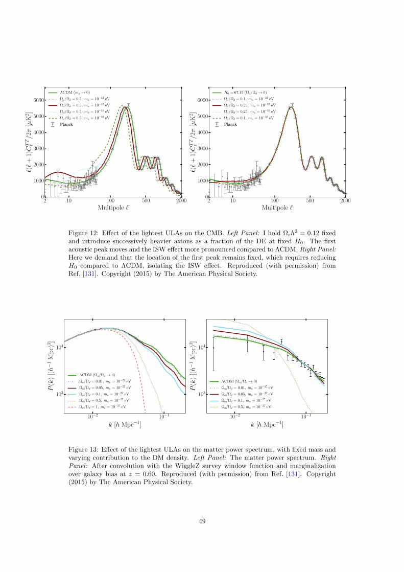
2 10 100 500 2000

Multipole `

0

1000

2000

3000

4000

5000

6000

`(`

+1)CTT

`/2π

[µK

2 ]

ΛCDM (ma → 0)

Ωa/Ωd = 0.5, ma = 10−33 eV

Ωa/Ωd = 0.5, ma = 10−32 eV

Ωa/Ωd = 0.5, ma = 10−31 eV

Ωa/Ωd = 0.5, ma = 10−30 eV

Planck

2 10 100 500 2000

Multipole `

0

1000

2000

3000

4000

5000

6000

`(`

+1)CTT

`/2π

[µK

2 ]

H0 = 67.15 (Ωa/Ωd → 0)

Ωa/Ωd = 0.1, ma = 10−32 eV

Ωa/Ωd = 0.25, ma = 10−32 eV

Ωa/Ωd = 0.25, ma = 10−31 eV

Ωa/Ωd = 0.1, ma = 10−30 eV

Planck

Figure 12: Effect of the lightest ULAs on the CMB. Left Panel: I hold Ωch2 = 0.12 fixed

and introduce successively heavier axions as a fraction of the DE at fixed H0. The firstacoustic peak moves and the ISW effect more pronounced compared to ΛCDM. Right Panel:Here we demand that the location of the first peak remains fixed, which requires reducingH0 compared to ΛCDM, isolating the ISW effect. Reproduced (with permission) fromRef. [131]. Copyright (2015) by The American Physical Society.

10−2 10−1

k [h Mpc−1]

103

104

P(k

)[(h−

1M

pc)

3 ]

ΛCDM (Ωa/Ωd → 0)

Ωa/Ωd = 0.01, ma = 10−27 eV

Ωa/Ωd = 0.05, ma = 10−27 eV

Ωa/Ωd = 0.1, ma = 10−27 eV

Ωa/Ωd = 0.5, ma = 10−27 eV

Ωa/Ωd = 1, ma = 10−27 eV

10−2 10−1

k [h Mpc−1]

103

104

P(k

)[(h−

1M

pc)

3 ]

ΛCDM (Ωa/Ωd → 0)

Ωa/Ωd = 0.01, ma = 10−27 eV

Ωa/Ωd = 0.05, ma = 10−27 eV

Ωa/Ωd = 0.1, ma = 10−27 eV

Ωa/Ωd = 0.5, ma = 10−27 eV

Figure 13: Effect of the lightest ULAs on the matter power spectrum, with fixed mass andvarying contribution to the DM density. Left Panel: The matter power spectrum. RightPanel: After convolution with the WiggleZ survey window function and marginalizationover galaxy bias at z = 0.60. Reproduced (with permission) from Ref. [131]. Copyright(2015) by The American Physical Society.

49

DM). The galaxy bias, b, changes the character of the effect. Galaxy bias is measured bythe survey by allowing b to float as a free parameter. When it varies, it can compensate, ina scale-independent manner, for suppression of power. The preferred value of b, and so thenormalization of the power spectrum, is thus different for the ULA cosmologies than forΛCDM, and this partial degeneracy reduces the constraining power of the galaxy survey.

The scale-dependent clustering of ULAs tells us that a full treatment of bias in thesecosmologies should involve computing a scale-dependent bias, b(k), and its dependence onthe ULA transfer function and growth rate. Scale-dependent bias in mixed DM cosmolo-gies is a poorly understood problem, and it has particular relevance to studies of massiveneutrinos (see e.g. Ref. [220]). Scale-dependent bias can be studied through numerical sim-ulation, or semi-analytically via the halo model [221]. Ref. [131] proposed an approximatetreatment of scale-dependent bias for ULAs, motivated by treatments of DE and neutrinos,and by the data, which we now outline.

Bias relates the galaxy power spectrum to the matter distribution. On scales whereULAs do not cluster (below the Jeans scale), we do not expect any correlation betweenthe galaxies and the ULAs. Galaxy surveys only observe out to some smallest wavenumber(largest scale), kobs. The scale of the observations defines an epoch, kobs = abiasH(abias):ULAs which only begin to behave like matter after this epoch will not be correlated withthe galaxy distribution on observable scales. We can approximate the scale of structuresuppression for ULAs as kosc = aoscH(aosc) and impose scale-dependent bias as a hard cutby excluding ULAs from the matter density if aosc > abias:

δρm = Θ(aosc − abias)(δρc + δρb) + Θ(abias − aosc)(δρc + δρb + δρa) , (137)

where Θ(x) is the Heaviside function, and ρm in the overdensity is defined in the samemanner. Because no current galaxy surveys observe on scales larger than the horizon size atequality, Ref. [131] made the simplification abias = aeq, which effectively removes ULAs fromthe matter distribution used to compute the galaxy power spectrum for ma . 10−27 eV.

An unbiased tracer of the matter distribution is provided by gravitational lensing. Up-coming surveys such as Euclid propose to measure the galaxy shear power spectrum [222],and could improve constraints on DM models considerably [172, 223, 224] if systematicscan be controlled. The forecasted sensitivity to Ωa of the lightest ULAs for a Euclid -likesurvey is shown in Fig. 14.33 These optimistic forecasts for weak lensing show an increasein sensitivity of around a factor of ten compared to the galaxy redshift survey alone.

The effect of axions on the expansion rate is also seen in the power spectrum, andis particularly evident if axions replace Λ (although now the issue of bias becomes morecomplicated [131]). This changes the age of the Universe relative to ΛCDM, with a youngerUniverse having less time to grow structures, reducing the amplitude of P (k). In the CMBthe effect of a younger Universe could be largely compensated by reducing H0; in P (k) itcan be compensated by changing the amplitude of primordial fluctuations, As. However, asboth the CMB and P (k) share common parameters, no choice of As and H0 can completelyremove the effects of this change, demonstrating the complementarity of CMB and LSSmeasurements. See Ref. [131] for further discussion.

5.3 Combined Constraints

Fig. 15 (left panel) shows the constraints on the axion dark sector density fraction, Ωa/Ωd,as a function of axion mass for CMB and CMB+WiggleZ data set combinations, takenfrom Ref. [131]. Including LSS data from WiggleZ as well as the CMB loosens constraintsslightly at low mass, and tightens them slightly at high mass. The looser constraint atlow mass is possibly being driven by the CMB/LSS tension in measurements of the power

33In this figure, neutrino parameters are included and marginalized over, lowering the CMB sensitivitycompared to that found in Ref. [131] (see next section, and Appendix F).

50

10−32

10−31

10−30

10−29

100

101

102

103

104

Fiducial Axion Mass [eV]

Un

cert

ain

ty i

n f a

x [P

erce

nt]

CMBGRSWLTotal

100

101

102

103

ma [eV]

(

a/

d)

Figure 14: Forecasted sensitivity of a Euclid -like galaxy redshift (GRS) and weak lensing(WL) survey to axion DM fraction, Ωa/Ωd, as a function of mass. WL increases sensitivityto Ωa by a factor of around ten compared to GRS alone. Reproduced and modified (withpermission) from Ref. [172]. Copyright (2012) by The American Physical Society.

32 31 30 29 28 27 26 25 24

log10(ma /eV)

0.2

0.4

0.6

0.8

1.0

Ωa/Ω

d

Axion as Dark energy Axion asDark matter

Constrained Region

CMBCMB + WiggleZ

!32 !30 !28 !26 !24 !22log10(ma/eV)

0.2

0.4

0.6

0.8

1.0

!a/

!d

!2.4

!2.1

!1.8

!1.5

!1.2

!0.9

!0.6

!0.3

0.0

log 1

0(" i

/Mpl)

Figure 15: Constraints to the axion dark sector energy fraction, Ωa/Ωd, as a function ofaxion mass from linear cosmological probes. Left Panel: Contours show 2 and 3 σ allowedregions comparing CMB and CMB+WiggleZ. Right Panel: CMB constraints, with samplepoints from chains colour-coded by axion initial displacement in Planck units. Reproduced(with permission) from Ref. [131]. Copyright (2015) by The American Physical Society.

51

spectrum amplitude (commonly expressed as the “σ8 tension”). The tighter constraint athigh mass is due to the WiggleZ data points with small error bars at k ∼ 0.1hMpc−1.

The normalization is Ωd = Ωa + Ωc, i.e. we consider a mixed DM model with CDMand ULAs. The allowed value at the lowest ULA masses, ma ≈ 10−33 eV, is Ωa/Ωd = 0.6implying Ωa ≈ 0.6, with the CDM density held fixed at close to its usual value. TheseULAs are DE and drive the current period of accelerated expansion. At high mass, wesee that in order for axions to be all the DM, with Ωa/Ωd = 1, requires ma ≥ 10−24eVat 95% C.L. This is the lower bound on DM particle mass from linear cosmological probes,as promised in the abstract. The constraint in the central, intermediate mass, region of10−32 eV ≤ ma ≤ 10−25.5 eV is Ωa/Ωd ≤ 0.05 and Ωah

2 ≤ 0.006 at 95%-confidence. Thatis, intermediate mass axions must make up less then 5% of the total DM.

It is important to note that the constraints of Ref. [131] apply to a cosmology with CDMplus a single light axion, and not to CDM plus multiple axions. It might be a good guess toassume that the constraint on the energy density in the intermediate mass regime appliesto the sum total energy density for all such axions (because the constraint is independentof mass). A dedicated study is necessary, but degeneracies will be even more problematicand a prudent choice of priors and sampling will be required (see Appendix F).

Fig. 15 (right panel) shows the CMB only constraints, with sample points from Multi-nest [225] chains colour-coded by the initial axion field displacement in Planck units (andre-sampled such that point density is proportional to probability as in a Markov chainMonte Carlo, MCMC).34 The field displacement is always φi < πMpl, and is thus consis-tent with a quadratic potential and sub-Planckian fa. Axion DE requires fa ∼ Mpl. Forma = 10−22 eV to be all the DM requires φi ∼ O(few)×1016 GeV. This shows that a ULAwith fa ≤ 1016 GeV will satisfy all current constraints on Ωa without fine tuning. Theseconclusions from numerical computation and full comparison with CMB data agree withthe discussion in Section 4.3.1 based on Eq. 61.

5.4 Isocurvature and Axions as a Probe of Inflation

Axions in the broken PQ scenario pick up isocurvature perturbations. The amplitude ofthese perturbations is proportional to the energy scale of inflation. The CMB places strongconstraints on the allowed amplitude of such perturbations. Therefore, if axions composethe DM, constraints on isocurvature constrain the energy scale of inflation, and a detectionof both would uniquely probe inflation. An independent measurement of the energy scaleof inflation can be used to place strong constraints on axion cosmology.

Let’s flesh these ideas out and quantify the possibilities. All of this Section assumesstandard, single-field, slow-roll inflation. We’ll focus on the QCD axion, which is alsocovered in detail in Refs. [134, 226, 141]. The case of ALPs is slightly more complicatedthan for the QCD axion, as the parameter space has more dimensions. ALPs are coveredby Refs. [211, 212, 66].

Axion isocurvature density perturbations are of uncorrelated CDM type, as long as theJeans scale can be neglected, which is the case for the QCD axion. The isocurvature CMBspectrum is shown in Fig. 16, where the effect of non-negligible ULA Jeans scale is alsoshown. The isocurvature power spectrum generated by Eq. (42) is:

PI = AI

(k

k0

)1−nI, (138)

with amplitude

AI =

(ΩaΩd

)2(HI/Mpl)

2

π2(φi/Mpl)2. (139)

34The field displacement is found by using Eq. (61) as the initial guess in a shooting method to obtainthe desired Ωa. We solve the Klein-Gordon equation at early times, switching to ρa ∝ a−3 when 3H = ma.

52

101 102 103

Multipole `10−6

10−5

10−4

10−3

10−2

10−1

100

101

102

103

104

`(`

+1)

C`/

2π[µ

K2 ]

increasing ma

10−4 = (0.01)2

Figure 16: CMB adiabatic and isocurvature spectra. ΛCDM adiabatic (dashed), CDMisocurvature with Ωa/Ωd = AI/As = 1 (dot dashed), ULA isocurvature with Ωa/Ωd = 0.01and increaing ma from left to right (solid, colour). Reproduced (with permission) fromRef. [211]. Copyright (2013) by The American Physical Society.

The scalar power is:

Pζ = As

(k

k0

)1−ns, (140)

with amplitude

As =1

2εinf

(HI

2πMpl

)2

= 2.20× 10−9 . (141)

The measured value of As is taken from Planck (2015), and the scalar spectral index ismeasured to be ns = 0.96 [105]. Uncorrelated CDM isocurvature is constrained to35

AIAs

< 0.038 . (142)

The tensor-to-scalar ratio, rT = 16εinf , provides an independent constraint on the energyscale of inflation. Planck and BICEP2 [86] provide the limit rT < 0.12. The projectedsensitivity of CMB-S4 experiments is rT ∼ 10−3 [229], while futuristic sensitivity from21cm lensing could be as low as rT ∼ 10−9 [230, 231].

All of these results are collected together for the QCD axion in Fig. 17. I plot contours forAI/As = 0.04 and Ωah

2 = 0.12 as functions of (fa, HI) at fixed levels of fine tuning on θa,i.Satisfying relic density and isocurvature constraints requires being below the intersectionsof these curves. For example, having θa,i = 1 and Ωah

2 = 0.12, requires fa ≈ 3×1011 GeV.The isocurvature constraint then enforces HI . 107 GeV. The intersection of the AIand Ωa constraints traces out, approximately, HI . 1010(fa/Mpl)

1/2 GeV if axions are

35This assumes scale invariance of the isocurvature power, ε 1, which is consistent with the impliedvalue of HI and rT . Compare this to the isocurvature power generated in the unbroken PQ scenario. Inthis case the amplitude is huge, AI ∼ 〈(δθ/θ)2〉 ∼ O(1) As, but power is only generated on very smallscales, k k0, that are not constrained by the CMB power spectrum. Spectral distortions and miniclustersmay impose interesting additional constraints [227, 228].

53

10 12 14 16 18

6

8

10

12

14

log10(fa/GeV)

log10(H

I/G

eV)

PQ

unbr

oken

AI

rT

i = 1

i = 102

i = 104

dh2

Allowed'(all'DM,'broken'PQ)'

Figure 17: The QCD axion and CMB tensor modes. The unbroken PQ scenario producesno isocurvature, and is allowed as long as the limits on rT and relic density (see Fig. 7) aresatisfied, requiring low fa. In the broken PQ scenario, we show various levels of tuning:θa,i = 1 (solid lines), θa,i = 10−2 (dashed lines), θa,i = 10−4 (dotted lines). Constraintsare shown for relic density Ωdh

2 < 0.12 (blue, lie below-left) and isocurvature amplitudeAI/As < 0.04 (red, lie below). The observable range of 10−9 < rT < 0.1 is shown in purple,with a realistic near-future limit of rT = 10−3 given by the solid line at HI ∼ 1013 GeV.The allowed regime if the QCD axion in the broken PQ scenario is to be all the DM is givenby the intersections of the red and blue lines (black), which always lies below a detectabletensor mode.

54

to be all the DM. The constraint quoted by Planck [96] in this scenario is HI < 0.86 ×107 GeV(fa/1011 GeV)0.408 (95% C.L.), consistent with our rough estimates.

A range of measurably-large values of rT are shown shaded purple, corresponding to arange 1010 GeV . HI . 1014 GeV. There is nowhere on the (fa, HI) plane where the QCDaxion in the broken PQ scenario can be all of the DM, satisfy iscourvature bounds, andproduce rT > 10−9 (a realistically observable value, shown by the dark purple line). Notethat such small values of r can be obtained, consistent with As and ns observations, instring inflation scenarios such as KKLT [232] or brane inflation (see Ref. [233] for details).

Relaxing the assumption that the QCD axion is all the DM, Fig. 17 shows that withθa,i . 10−4 a range of large fa starts to become consistent with rT > 10−9. By trialand error, we find the maximum value of rT consistent with isocurvature constraints andfa < Mpl occurs for θa,i ≈ 10−7 where we have Ωah

2 < 10−6 and rT ≈ 10−4. There is noamount of tuning that can make the QCD axion in the broken PQ scenario consistent withtensor modes as large as rT = 10−3, the CMB-S4 target.

CDM-type isocurvature modes are avoided completely in the unbroken PQ scenario.Thus, if tensor modes are observed, the QCD axion must live in the parameter space ofFig. 7 contained within the grey shaded region of Fig. 17, implying fa < 1011 GeV.

These conclusions can be avoided if some of our cosmological assumptions are relaxed.An example non-minimal inflation model producing rT > 10−3 consistent with the brokenPQ scenario and high fa, uses the radial PQ field, χ, as the inflaton, non-minimally coupledto gravity (similarly to Higgs inflation) [234]. Such a scenario can allow for simultaneousdetection of DM axions by CASPEr [235] (see Section 9.5.2), and detection of rT by, e.g.,spider [236]. There are many other possibilities to avoid the isocurvature problem of high-scale axions by modifying inflation, particle physics, or the thermal history, for exampleRef. [237], and related works.

We conclude our discussion of the QCD axion and isocurvature in summary:

• The QCD axion in the broken PQ scenario is incompatible with observably-large tensormodes from standard inflation.36

• In the broken PQ scenario with standard inflation, axion isocurvature modes couldprobe HI as low as 107 GeV, offering a unique probe of low-scale inflation.

• Simultaneously detecting a high fa & 1013 GeV QCD axion and tensor modes atrT = 10−3 would falsify minimally coupled, single-field, slow-roll inflation with astandard thermal history.

6 Galaxy Formation

This section reviews work presented in Refs. [178, 238, 239].

6.1 The Halo Mass Function

The halo mass function (HMF) gives the expected number of halos per logarithmic massbin, per unit volume, for a given cosmology. It depends fundamentally on two quantities,both of which can depend on halo mass and redshift: the variance of fluctuations, σ2(M, z),and the linearly extrapolated critical density required for such fluctuations to collapse,δcrit(M, z). The relevant standard formulae are given in Appendix G.

We can compute σ(M, z) given the linear power spectrum, P (k, z). The cut-off in powercaused by the axion Jeans scale leads to a suppression of σ(M, z) compared to CDM at

36It is, in fact, possible to make the QCD axion in the broken PQ scenario compatible with observabletensors if we allow fa & 1010Mpl and tune the initial misalignment angle at a level θa,i 10−10. I excludesuch a scenario as unreasonable. The tuning is worse than the strong-CP problem, and the existence of ascale so much larger than the Planck scale is considered highly problematic in theories of quantum gravity.

55

low halo mass, with σ(M, z) going to a constant as M → 0. The reduced value of σ(M, z)reduces the abundance of low mass halos.

In an Einstein-de Sitter universe (CDM with Λ = 0), spherical collapse can be solvedexactly. Scale-independent growth gives a constant, mass-independent, value for δcrit, whichcan be scaled to any redshift using the linear growth factor (the result also works well forΛCDM on not-too-large scales):

δcrit,EdS(z) =1.686D0

D(z). (143)

The collapse barrier is mass-independent for CDM because the growth equation isscale-invariant. In DM models with an effective pressure, the Jeans scale introduces scale-dependence into the collapse threshold. In spherical collapse simulations with WDM, wherefree-streaming was modelled by an effective pressure [240], a mass-dependent critical barrieris found, with δcrit increasing below the WDM Jeans scale. This barrier can then be used ina full excursion set model of WDM halo formation, dramatically suppressing halo formationbelow the effective Jeans mass [241]. Spherical collapse and the excursion set have not beenstudied for axion DM. Instead, Ref. [178] proposed a simple model where D(z) in Eq. (143)is simply replaced by an appropriately normalized (in both scale and redshift relative toΛCDM) scale-dependent growth factor, G. The mass can be assigned from the wavenumberusing the enclosed mean density in a sphere of radius R = π/k giving:

δcrit(M, z) = 1.686G(M, z) . (144)

We define G as the relative amount of growth between axion DM and CDM, normalizedto unity on large scales, k0, and at early times, zearly:

G(k, z) =δa(k0, z)δa(k, zearly)

δa(k, z)δa(k0, zearly)

δc(k, z)δc(k0, zearly)

δc(k0, z)δc(k, zearly), (145)

where δa is computed in the axion cosmology, and δc is computed in the CDM cosmology,with Ωah

2 = Ωch2. In practice, k0 should be chosen such that k0 < kJ(zearly), but not so

small such that scale dependent growth in ΛCDM due to Λ domination becomes relevant.Similarly, zearly should be chosen such that the power spectrum shape in ΛCDM has frozenin, i.e. after BAO formation. For DM axions in a close-to-ΛCDM cosmology, reasonablechoices are k0 = 0.002hMpc−1 and zearly ≈ 300.37

The critical overdensity appears in the HMF in the argument of a Gaussian. Thus, evena modest increase in δcrit causes a sharp cut-off in the HMF: this is shown in Fig. 18.38 Thecut-off makes physical sense: there are no seed density perturbations on scales below theJeans scale, and even if there were, growth is so suppressed there that density perturbationscannot collapse into virialized objects. At higher redshifts, when density perturbations aresmaller, and the Jeans scale is larger, the effect is more pronounced. We learn that: ULAsdramatically suppress halo formation compared to CDM at low halo masses and at highredshifts.39

For the QCD axion, the cut-off in the HMF induced by the Jeans scale is on extremelysmall scales M < 10−9M (c.f. the standard WIMP, where the smallest halos have mass

37An interesting recent discussion of the relative importance of scale dependent growth to LSS simulationsof axion DM is given in Ref. [188], where a similar quantity to G is used to measure this.

38The fact that the barrier appears in a Gaussian also renders the details of the barrier function, such asthe acoustic features and smoothing scheme at masses much below the axion Jeans scale, largely irrelevantfor halo statistics.

39There is some discussion and debate concerning the location and origin of the HMF cut-off in bothWDM (filtering, spurious structure [191]) and CDM (baryonic effects) that I will not go into here. Foraxions, numerical simulations such as those of Ref. [199, 188], with the addition of hydrodynamics and starformation, are necessary in order to be more precise. For basic, semi-analytic results, the intuitive notionof a cut-off at the Jeans scale provided by scale-dependent growth is sufficient.

56

107 108 109 1010 1011 1012 1013 1014

M [M]

100

101

102

δ cri

t[D

(z)/D

0]

107 108 109 1010 1011 1012 1013 1014

M [M]

10−13

10−8

10−3

102

dn

dlnM

[(M

pc)−

3 ]

CDMma = 10−22 eV

14

7

0

Red

shif

tz

Figure 18: Right Panel: Critical overdensity for collapse, δcrit(M, z) for ma = 10−22 eVcomputed from scale-dependent growth using Eq. (144), normalizing for the growth inΛCDM using D(z). Left Panel: Resultant halo mass function, compared to CDM. Modifiedfrom Ref. [238], Figs. 1 and 2.

M ≈ 10−6M [179]). These smallest halos will certainly be tidally disrupted today, butare interesting to study the very first moments of structure formation at z ≈ 60 in CDMmodels. Axion miniclusters produced in the unbroken PQ scenario for the QCD axion inthe classic window have Mmc ≈ 10−9M [242]. Miniclusters of ALPs may be more, or less,massive. Being denser than ordinary halos, axion miniclusters survive to the present dayand are relevant to observational searches for minihalos (e.g. Refs. [227, 243, 244]).

6.2 Constraints from High-z and the EOR

There is accumulating data about the high-z Universe. We see a number of very highredshift galaxies with Hubble Ultra Deep Field (HUDF, e.g. Ref. [245]). We also knowthat the intergalactic medium (IGM) is reionized by star formation. Reionization is knownto be essentially complete by z ∼ 6 (e.g. observation of Gunn-Peterson trough [246] inquasar spectra [247]). Furthermore, reionization of the IGM produces an optical depth tothe CMB, which is constrained by a combination of large angle temperature and polar-ization correlation functions to be τ = 0.07–0.08 ± 0.02 (central value depends on datasetcombinations in Ref. [105]).

The suppression of halo formation at high-z by ULAs cannot be too severe, or else itwould be inconsistent with these observations, producing too few high-z galaxies to matchHUDF and to efficiently reionize the IGM. Getting these things right places a lower boundon ma if ULAs are to contribute significantly to the DM density. Ref. [238] investigatedthese bounds, following similar work on WDM in Ref. [248].

In order to obtain constraints from the HMF, one needs to relate the halo mass tothe UV magnitude of the galaxy, MUV. This can be done by abundance matching [249,250]. The luminosity function, φlum(MUV, z), is fit and matched to the low-z observations.The integrated (cumulative) luminosity function is then matched by number count to thecumulative halo mass function: Φlum(< MUV, z) = n(> Mh, z). This chain of relationsfixes Mh(MUV). Therefore, once the low redshift data are fixed, the high redshift value ofΦlum(MUV, z) can be predicted for a given DM model, and itself compared to observation.The cut-off in the HMF induced by the axion Jeans scale cuts off the Mh(MUV) relation atsome brightest magnitude, leaving the function Φlum(MUV, z) with no support at the faint

57

−22 −20 −18 −16 −14 −1210−6

10−5

10−4

10−3

10−2

10−1

MUV

Φ(<

MUV)[1/

Mpc]

3

CDM, 1 CDM, 210−22eV, 110−22eV, 210−22eV, 310−22eV, 410−23eV, 310−23eV, 4

z = 8

4 6 8 10 12 140

0.2

0.4

0.6

0.8

1

z

Q

aMDM, 10−22eVaMDM, 10−21eVCDM, 1aCDM, 1d

Figure 19: Left Panel: Cumulative UV luminosity at z = 8, here denoted Φ, in axionmodels using the abundance matching technique. Data: HUDF [245]. Dashed line: JWSTreach [251]. Model numbers are different abundance matching procedures and DM compo-sition. Models 1, 2, ULAs are all the DM. Models 3, 4, ULAs are half of the DM. RightPanel: Ionization fraction. Shaded regions cover model uncertainties. Only extreme edgesshown for CDM. Reproduced from Ref. [238], Figs. 4 and 6.

end.Fig. 19 (Left Panel) shows the predicted cumulative luminosity function for axion DM

at z = 8. If ULAs are too light, or make up too much of the DM, it is impossible to matchthe observed HUDF UV luminosity. The model ma = 10−23 eV with Ωah

2 > 0.06 is ruledout at > 8σ by HUDF. The model ma = 10−22 eV with Ωah

2 = 0.12 is consistent withHUDF, but only just: the UV luminosity function cuts off at MUV ≈ −18, right wherethe constraint is. This model could be excluded by a JWST measurement of the faint-endluminosity function at MUV ≈ −16 [251] if it were found to be consistent with the largerCDM value of Φlum(MUV, z).

The UV luminosity function can also be used to predict the evolution of the ionizationfraction, Q(z) (not to be confused with the quantum potential, also denoted Q). Thisinvolves a fair amount of astrophysical modelling, as described in e.g. Refs. [252, 238, 188].The results are shown in Fig. 19 (Right Panel), with shaded regions showing modellinguncertainty. These results are broadly consistent with the studies of Refs. [188, 189], wherethe underlying halo mass function was computed from N -body simulations with modifiedinitial power spectra. Ref. [189] also used different methods to model the reionization field.

The ionization fraction gives the optical depth to redshift, τ(z), from the integral alongthe line of sight:

τ(z) =

∫ z

0

dz′(1 + z′)2

H(z′)Q(z′)σT nH(1 + ηHeY/4X) , (146)

where σT is the Thompson optical depth, nH is the mean comoving Hydrogen numberdensity, Y = (1 − X) is the Helium fraction, X is the Hydrogen fraction, and ηHe isthe ionization state of Helium (see Ref. [238] for references and more details on theseparameters). The optical depth to the CMB is τ(zrec ≈ 1100).

Ref. [238] found that, within the modelling uncertainty, all axion DM models withma ≥ 10−22 eV can reproduce a CMB optical depth consistent with observations, whilema = 10−23 eV cannot (though the tension for the lightest masses is slightly less with therevised, Planck 2015, value for the optical depth). Thus the CMB optical depth excludesthe lightest ULAs with ma . 10−23 eV from being all of the DM.

58

There is the opportunity in future to constrain axion DM with ma ∼ 10−22–10−21 eVfrom the evolution of Q(z). The cut off in the HMF delays the formation of the firstgalaxies, and thus reionization occurs at lower redshift than in CDM. Once collapse hasbegun, structure builds up more rapidly for ULAs, and reionization completes in a smallerredshift window. These different reionization histories distinguish ULAs and CDM. Forexample, the amplitude of the kinetic Sunyaev-Zel’dovich effect [253] in the CMB is sensitiveto the duration of reionization (e.g. Ref. [254]). This will be measured in the near futureby Advanced ACTPol [255] and could distinguish ma . 10−21 eV from CDM [238].

The bottom line is that high-z constraints currently exclude ma = 10−23 eV from be-ing all of the DM at high confidence, and ma = 10−22 eV is right on the edge of ac-ceptability. The bounds are only approximate, as a lot of uncertain astrophysics is in-volved, but Ref. [238] covered a range of models and the lower limit on ma & 10−22 eVis reliable by order of magnitude. Similar results were also found by Ref. [188], givingma ≥ 1.2 × 10−22 eV (2σ). This is the current lower limit on DM particle mass fromnon-linear clustering. Future constraints on high-z galaxies, and on the mean redshift andduration of reionization, could improve this limit by some two or more orders of magnitude.A measurement of the large scale 21cm power spectrum could constrain ULA mass as highas ma ≈ 10−18 eV [182].

6.3 Halo Density Profiles

N -body simulations of pure CDM indicate that halo density profiles have a universal shape,known as the Navarro-Frenk-White (NFW) profile [256]:

ρNFW(r)

ρcrit.=

δNFW

r/rs(1 + r/rs)2, (147)

where δNFW is a function of the “halo concentration,” commonly denoted as c, and rs isthe scale radius. The concentration is defined such that the virial radius is rvir = crs.

40

Notice that the NFW halo is a smoothly varying power law, with ρ ∼ r−1 in the centre:the so-called ‘cusp.’

A dwarf galaxy in ΛCDM with M ∼ 1010M has peak circular velocity on the orderof 50 km s−1 at a radius of around 10 kpc. The de Broglie wavelength, λdB = 1/mv, of aparticle inside such galaxy is then

λdB ≥ 4× 10−2( ma

10−22 eV

)−1

kpc , (148)

and for a ULA is non-negligible in terms of the galaxy size. Using that v ∼ M/r and

M ∼ ρr3, setting λdB = r we find that λdB ∼ m−1/2a ρ−1/4 ∼ rJ where rJ is the Jeans scale.

Let’s work directly with the Jeans scale. Taking rJ = 2π/kJ and simply scaling Eq. (101)to the halo density gives

rJ = 94.5( ma

10−22 eV

)−1/2(ρ(rJ)

ρcrit.

)−1/4(Ωah

2

0.12

)−1/4

kpc . (149)

This is a polynomial equation to be solved for rJ . Plugging in a typical overdensity of 106

with ma = 10−22 eV gives rJ ∼ 3 kpc. The ULA Jeans scale inside a dwarf halo can bevery large.

The wavelike effects of ULAs (the de Broglie and Jeans scales) affect the halo densityprofile, and it cannot be completely described by the CDM result. How is the NFW profilemodified by the presence of a ULA and what forms on small scales? Clearly there should be

40The virial radius is taken to be the radius where the density is 200 times the critical density, and thevirial velocity is the circular velocity at this radius. The mass of a halo is often defined as M200 = M(< rvir).One can use this to derive δNFW(c). A typical concentration is c ∼ 10.

59

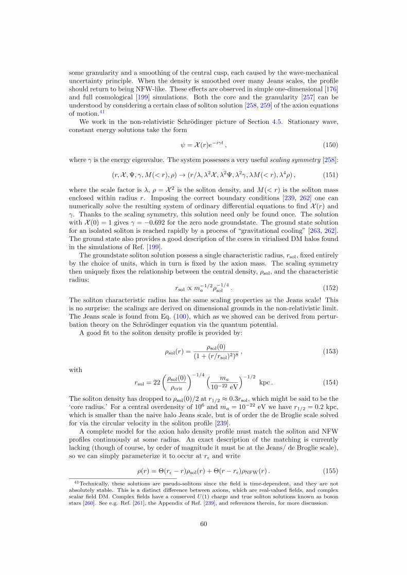
some granularity and a smoothing of the central cusp, each caused by the wave-mechanicaluncertainty principle. When the density is smoothed over many Jeans scales, the profileshould return to being NFW-like. These effects are observed in simple one-dimensional [176]and full cosmological [199] simulations. Both the core and the granularity [257] can beunderstood by considering a certain class of soliton solution [258, 259] of the axion equationsof motion.41

We work in the non-relativistic Schrodinger picture of Section 4.5. Stationary wave,constant energy solutions take the form

ψ = X (r)e−iγt , (150)

where γ is the energy eigenvalue. The system possesses a very useful scaling symmetry [258]:

(r,X ,Ψ, γ,M(< r), ρ)→ (r/λ, λ2X , λ2Ψ, λ2γ, λM(< r), λ4ρ) , (151)

where the scale factor is λ, ρ = X 2 is the soliton density, and M(< r) is the soliton massenclosed within radius r. Imposing the correct boundary conditions [239, 262] one cannumerically solve the resulting system of ordinary differential equations to find X (r) andγ. Thanks to the scaling symmetry, this solution need only be found once. The solutionwith X (0) = 1 gives γ = −0.692 for the zero node groundstate. The ground state solutionfor an isolated soliton is reached rapidly by a process of “gravitational cooling” [263, 262].The ground state also provides a good description of the cores in virialised DM halos foundin the simulations of Ref. [199].

The groundstate soliton solution possess a single characteristic radius, rsol, fixed entirelyby the choice of units, which in turn is fixed by the axion mass. The scaling symmetrythen uniquely fixes the relationship between the central density, ρsol, and the characteristicradius:

rsol ∝ m−1/2a ρ

−1/4sol . (152)

The soliton characteristic radius has the same scaling properties as the Jeans scale! Thisis no surprise: the scalings are derived on dimensional grounds in the non-relativistic limit.The Jeans scale is found from Eq. (100), which as we showed can be derived from pertur-bation theory on the Schrodinger equation via the quantum potential.

A good fit to the soliton density profile is provided by:

ρsol(r) =ρsol(0)

(1 + (r/rsol)2)8, (153)

with

rsol = 22

(ρsol(0)

ρcrit

)−1/4 ( ma

10−22 eV

)−1/2

kpc . (154)

The soliton density has dropped to ρsol(0)/2 at r1/2 ≈ 0.3rsol, which might be said to be the‘core radius.’ For a central overdensity of 106 and ma = 10−22 eV we have r1/2 = 0.2 kpc,which is smaller than the naive halo Jeans scale, but is of order the de Broglie scale solvedfor via the circular velocity in the soliton profile [239].

A complete model for the axion halo density profile must match the soliton and NFWprofiles continuously at some radius. An exact description of the matching is currentlylacking (though of course, by order of magnitude it must be at the Jeans/ de Broglie scale),so we can simply parameterize it to occur at rε and write

ρ(r) = Θ(rε − r)ρsol(r) + Θ(r − rε)ρNFW(r) . (155)

41Technically, these solutions are pseudo-solitons since the field is time-dependent, and they are notabsolutely stable. This is a distinct difference between axions, which are real-valued fields, and complexscalar field DM. Complex fields have a conserved U(1) charge and true soliton solutions known as bosonstars [260]. See e.g. Ref. [261], the Appendix of Ref. [239], and references therein, for more discussion.

60

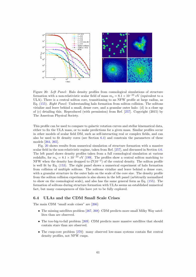
Figure 20: Left Panel: Halo density profiles from cosmological simulations of structureformation with a non-relativistic scalar field of mass ma = 8.1× 10−23 eV (equivalent to aULA). There is a central soliton core, transitioning to an NFW profile at large radius, asEq. (155). Right Panel: Understanding halo formation from soliton collision. The solitonsvirialize and leave behind a small, dense core, and a granular outer halo: (d) is a close upof (c) detailing this. Reproduced (with permission) from Ref. [257]. Copyright (2015) byThe American Physical Society.

This profile can be used to compare to galactic rotation curves and stellar kinematical data,either to fix the ULA mass, or to make predictions for a given mass. Similar profiles occurin other models of scalar field DM, such as self-interacting real or complex fields, and canalso be used to fit density cores (see Section 6.4) and constrain the parameters of thesemodels [264, 265].

Fig. 20 shows results from numerical simulation of structure formation with a massivescalar field in the non-relativistic regime, taken from Ref. [257], and discussed in Section 4.6.The left panel shows density profiles taken from a full cosmological simulation at variousredshifts, for ma = 8.1 × 10−23 eV [199]. The profiles show a central soliton matching toNFW when the density has dropped to O(10−2) of the central density. The soliton profileis well fit by Eq. (153). The right panel shows a numerical experiment of halo formationfrom collision of multiple solitons. The solitons virialize and leave behind a dense core,with a granular structure in the outer halo on the scale of the core size. The density profilefrom the soliton collision experiments is also shown in the left panel (arbitrarily normalizedto show on the cosmological scale), and also has the same general form as Eq. (155). Theformation of solitons during structure formation with ULAs seems an established numericalfact, but many consequences of this have yet to be fully explored.

6.4 ULAs and the CDM Small Scale Crises

The main CDM “small scale crises” are [266]:

• The missing satellites problem [267, 268]: CDM predicts more small Milky Way satel-lites than are observed.

• The too-big-to-fail problem [269]: CDM predicts more massive satellites that shouldcontain stars than are observed.

• The cusp-core problem [270]: many observed low-mass systems contain flat centraldensity profiles, not NFW cusps.

61

All of these problems, and variants of them, are essentially related to the overabundance ofstructure on small-scales in CDM, which itself is caused by the cold, collisionless, scale-freenature of CDM clustering.

Methods to address the small-scale problems come in two varieties: baryonic/astrophysicalsolutions, and dark matter solutions. A recent set of state-of-the-art simulations discussingthe baryonic solutions based on feedback from star formation is Ref. [271], while a reviewof the relevant issues if Ref. [272].

Dark matter based solutions are interesting, as they attempt to solve the problemsby the introduction of a small number of universal parameters. The extent to which thesemodels offer a solution can in principle point to specific values of these parameters. Becauseof this, we should not only demand solutions to the small-scale crises, but also a completeand consistent cosmological history, which gives the models some predictive power. Theyalso offer us a framework for parameterizing our uncertainty about DM. In the absence of afundamental theory of DM, as Bayesians we should allow for varying DM properties at thesame time as we vary the baryonic physics. Moving away from CDM in this way may allowfor a mixed baryon-DM solution with more reasonable priors on astrophysical parameters.Finally, a range of parameters will also be excluded, e.g. providing too few satellites, andindependent of offering a solution to the small-scale crises we have learned something newabout DM.

So what do DM solutions to the small-scale crises look like? Two popular models areself-interacting (SI)DM [273], and WDM [170]. I will only discuss WDM in detail, as it isinteresting to contrast with ULAs. For further discussion of SIDM and other interactingmodels with relation to the small-scale crises and other areas of galaxy formation, see e.g.Refs. [274, 275, 276, 277].

WDM suppresses structure formation by free-streaming and a cut-off in the matterpower, as we discussed in Section 4.4.5. This has the ability to address the missing satellitesand too-big-to-fail problems for 1.5 keV . mX . 2.3 keV [190], while still producing enoughsatellites and passing constraints on phase space density [280]. Fermion degeneracy pressureand thermal velocities also allow WDM to form density cores [281]. The core-size-WDM

mass relation is plotted in Fig. 21, with rc ∼ m−1/2X . Herein lies a problem known as

the Catch 22 of WDM [278]: core sizes in dwarf galaxies are too small if constraints fromsatellite abundance and LSS are accounted for. Specifically, the N-body simulations ofRef. [278] found that masses mX ∼1-2 keV gives a core of size rc ∼ 10(20) pc in a dwarfgalaxy of mass 1010(8)M, far smaller than the O(kpc) cores required in e.g. Fornax andSculptor [282]. Ref. [283] computed the WDM phase space density from N-body simulationsand used this to derive the core size expected from free-streaming. A mass mX ≈ 0.5 keVcan provide cores to the Milky Way dSphs, which is too light to be consistent with structureformation.

That an ultralight scalar field, such as an axion, could potentially also resolve the small-scale crises has been known for some time [284, 285, 176, 286]: the Jeans scale suppressesthe formation of low mass halos, and at the same time leads to density cores in the formof solitons, as we have already discussed. Here we will address one issue: do ULAs suffera Catch 22 like WDM does? The answer, in short, is “no,” or more accurately “not asseverely.”

Fig. 22 shows the one dimensional likelihood for ULA mass from fitting stellar velocitydispersion data of Ref. [282]. This simplified data uses two stellar populations and mea-sures only the slopes of the density profiles within a given radius, in principle allowing anarbitrarily large core outside of this (and hence arbitrarily low axion mass). However, thiswould allow arbitrarily large dSph mass, while masses M & O(few) × 1010M are forbid-den by their long dynamical friction time scales [287].42 In Fig. 22 the dynamical frictionconstraint is imposed as a hard prior, supplementing the density profile slope analysis [282]

42I compute the maximum mass for each dSph individually from the formula in Ref. [287] using theirco-ordinates [288] and an approximate circular velocity vc ≈ 200 km s−1.

62

Figure 21: Core size in a WDM halo of mass M = 5×108M as a function of WDM thermalrelic mass, with uncertainties given by the shaded region. A representative constraint ofmX > 2 keV is shown by the vertical dashed line, which leads to small, O(10 pc) cores andimposes the WDM Catch 22. Reproduced (with permission) from Ref. [278, 279], Fig. 2.

63

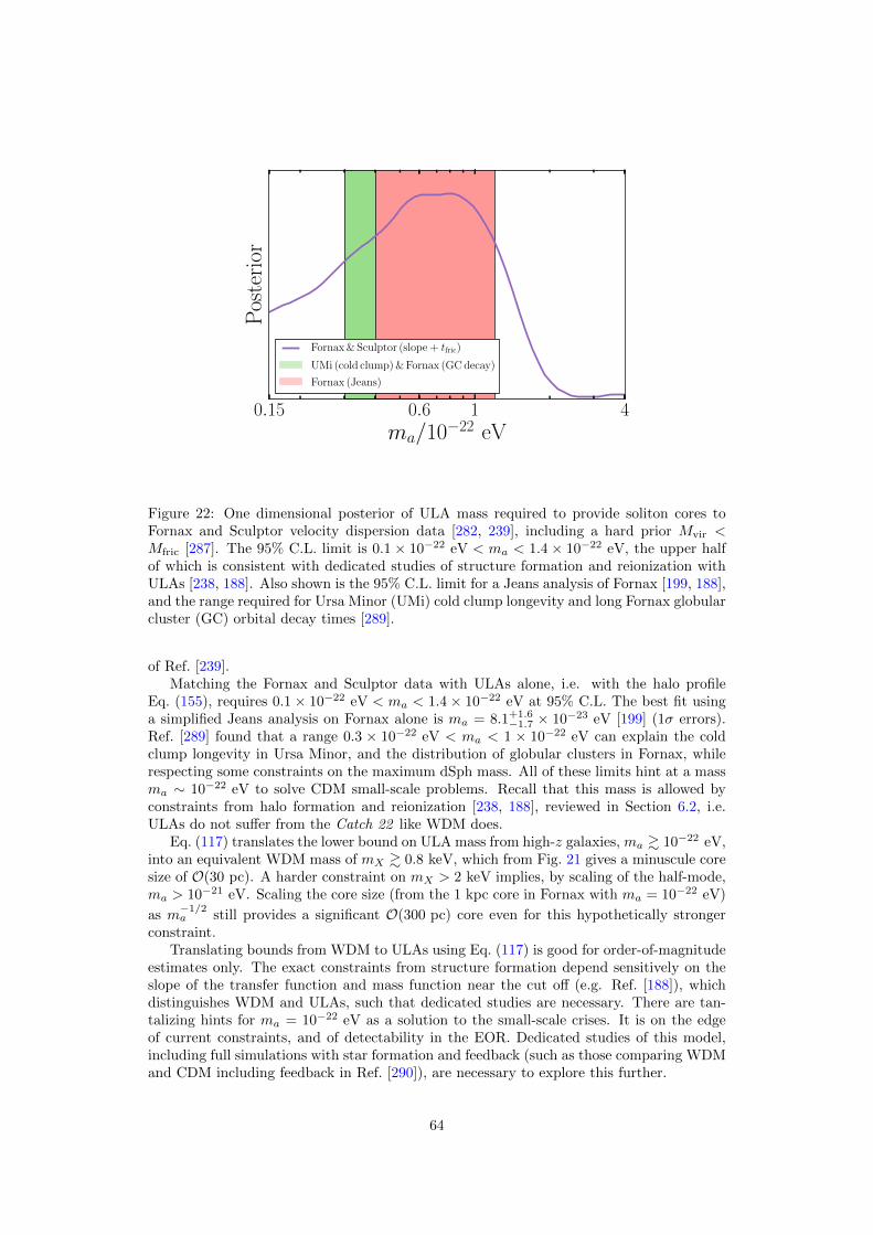
0.15 0.6 1 4

ma/10−22 eV

Pos

teri

or

Fornax & Sculptor (slope + tfric)

UMi (cold clump) & Fornax (GC decay)

Fornax (Jeans)

Figure 22: One dimensional posterior of ULA mass required to provide soliton cores toFornax and Sculptor velocity dispersion data [282, 239], including a hard prior Mvir <Mfric [287]. The 95% C.L. limit is 0.1 × 10−22 eV < ma < 1.4 × 10−22 eV, the upper halfof which is consistent with dedicated studies of structure formation and reionization withULAs [238, 188]. Also shown is the 95% C.L. limit for a Jeans analysis of Fornax [199, 188],and the range required for Ursa Minor (UMi) cold clump longevity and long Fornax globularcluster (GC) orbital decay times [289].

of Ref. [239].Matching the Fornax and Sculptor data with ULAs alone, i.e. with the halo profile

Eq. (155), requires 0.1× 10−22 eV < ma < 1.4× 10−22 eV at 95% C.L. The best fit usinga simplified Jeans analysis on Fornax alone is ma = 8.1+1.6

−1.7 × 10−23 eV [199] (1σ errors).Ref. [289] found that a range 0.3 × 10−22 eV < ma < 1 × 10−22 eV can explain the coldclump longevity in Ursa Minor, and the distribution of globular clusters in Fornax, whilerespecting some constraints on the maximum dSph mass. All of these limits hint at a massma ∼ 10−22 eV to solve CDM small-scale problems. Recall that this mass is allowed byconstraints from halo formation and reionization [238, 188], reviewed in Section 6.2, i.e.ULAs do not suffer from the Catch 22 like WDM does.

Eq. (117) translates the lower bound on ULA mass from high-z galaxies, ma & 10−22 eV,into an equivalent WDM mass of mX & 0.8 keV, which from Fig. 21 gives a minuscule coresize of O(30 pc). A harder constraint on mX > 2 keV implies, by scaling of the half-mode,ma > 10−21 eV. Scaling the core size (from the 1 kpc core in Fornax with ma = 10−22 eV)

as m−1/2a still provides a significant O(300 pc) core even for this hypothetically stronger

constraint.Translating bounds from WDM to ULAs using Eq. (117) is good for order-of-magnitude

estimates only. The exact constraints from structure formation depend sensitively on theslope of the transfer function and mass function near the cut off (e.g. Ref. [188]), whichdistinguishes WDM and ULAs, such that dedicated studies are necessary. There are tan-talizing hints for ma = 10−22 eV as a solution to the small-scale crises. It is on the edgeof current constraints, and of detectability in the EOR. Dedicated studies of this model,including full simulations with star formation and feedback (such as those comparing WDMand CDM including feedback in Ref. [290]), are necessary to explore this further.

64

7 Axions and Accelerated Expansion

7.1 Axions and the Cosmological Constant Problem

Our discussion in this review began with one of the greatest unsolved problems in modernphysics: the cosmological constant (c.c.) problem [1], one of the most notoriously hardproblems to solve in high energy physics [291]. One particularly attractive solution tothis problem is anthropic tuning, which can be realized by eternal inflation populating alarge number of vacua in the string landscape [292, 293] (the original idea dates back toRef. [294]). In this picture, four-form fluxes and topologically complex compact spaces withO(100) or more cycles both play important roles.43 Recall from Section 2.4 that axionsarise from the wrapping of such fluxes on cycles. Furthermore, the canonical axion potentialV (φ) ∝ cosφ/fa can provide positive and negative contributions to the vacuum energy,allowing axions to cancel contributions to the c.c. from other sources in a cosmologicallydynamical manner.

The above observations suggest that:

• Axions may play a central role in the solution of the c.c. problem.

• The anthropic solution of the c.c. problem in the string landscape provides goodmotivation for the existence of the axiverse.

In this section we will briefly discuss a few ideas relating axions to the c.c. problem.We begin with the simplest model of axion quintessence. As we already saw in Sec-

tion 5, ULAs with ma ∼ H0 ∼ 10−33 eV can act as DE, with the axion potential energyproviding an effective cosmological constant and driving accelerated expansion as a form ofquintessence. Since the axion mass is protected by a shift symmetry and can easily remainso light, the idea of axion and general pNGB [295] quintessence is natural, and has a longhistory [296].44

The model is specified by the potential

V (φ) = Λ4a

[1 + cos

(φ

fa

)], (156)

(note the phase shift from our previous definition). The most recent constraints on thisscenario using Planck data can be found in Ref. [298] and are summarized in Fig. 23. Sincethe vacuum in this potential has zero energy, the quintessence contribution to the energybudget, Ωφ, is controlled by the initial field displacement, φi. The value of Ωφ ≈ 0.69 iswell constrained by the requirement of driving accelerated expansion, and just as we saw inFig. 15 (right panel) large field displacements and decay constants are required to achievethis. There is a degeneracy between the energy density and the decay constant causedby the requirement of keeping the potential roughly flat compared to H0: increasing Λarequires increasing fa to retain flatness.

A simple generalization of this quintessence model goes along the lines of N -flation (seeSection 7.2.1), and was discussed in Ref. [58]. Taking the string theory-inspired potentialin Eq. (34) for N axions of almost degenerate mass, and assuming a fixed decay constant:

fa =Mpl

Sinst., (157)

it can be shown that axion quintessence requires

Sinst. ∼ 200− 300 and N & S2inst. , (158)

43This “100” is one origin of the famous statement that the string theory landscape contains 10500 vacua.In this context it arises from demanding that the number of vacua is densely enough distributed near theobserved value of the c.c. to make a universe in this region sufficiently likely.

44For a review of DE and quintessence models, see Ref. [297].

65

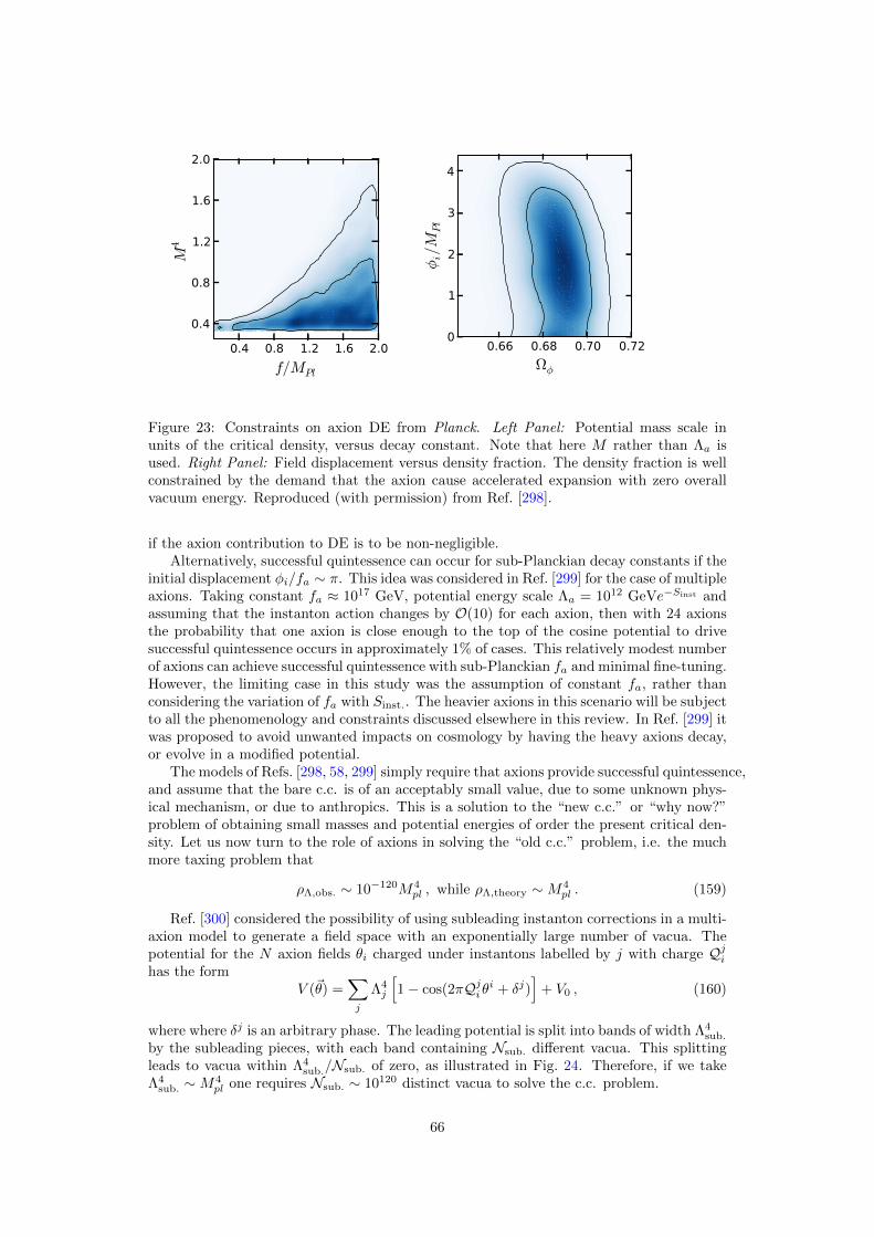
0.4 0.8 1.2 1.6 2.0f/MPl

0.4

0.8

1.2

1.6

2.0M

4

0.66 0.68 0.70 0.72Ωφ

0

1

2

3

4

φi/M

Pl

Figure 23: Constraints on axion DE from Planck. Left Panel: Potential mass scale inunits of the critical density, versus decay constant. Note that here M rather than Λa isused. Right Panel: Field displacement versus density fraction. The density fraction is wellconstrained by the demand that the axion cause accelerated expansion with zero overallvacuum energy. Reproduced (with permission) from Ref. [298].

if the axion contribution to DE is to be non-negligible.Alternatively, successful quintessence can occur for sub-Planckian decay constants if the

initial displacement φi/fa ∼ π. This idea was considered in Ref. [299] for the case of multipleaxions. Taking constant fa ≈ 1017 GeV, potential energy scale Λa = 1012 GeVe−Sinst andassuming that the instanton action changes by O(10) for each axion, then with 24 axionsthe probability that one axion is close enough to the top of the cosine potential to drivesuccessful quintessence occurs in approximately 1% of cases. This relatively modest numberof axions can achieve successful quintessence with sub-Planckian fa and minimal fine-tuning.However, the limiting case in this study was the assumption of constant fa, rather thanconsidering the variation of fa with Sinst.. The heavier axions in this scenario will be subjectto all the phenomenology and constraints discussed elsewhere in this review. In Ref. [299] itwas proposed to avoid unwanted impacts on cosmology by having the heavy axions decay,or evolve in a modified potential.

The models of Refs. [298, 58, 299] simply require that axions provide successful quintessence,and assume that the bare c.c. is of an acceptably small value, due to some unknown phys-ical mechanism, or due to anthropics. This is a solution to the “new c.c.” or “why now?”problem of obtaining small masses and potential energies of order the present critical den-sity. Let us now turn to the role of axions in solving the “old c.c.” problem, i.e. the muchmore taxing problem that

ρΛ,obs. ∼ 10−120M4pl , while ρΛ,theory ∼M4

pl . (159)

Ref. [300] considered the possibility of using subleading instanton corrections in a multi-axion model to generate a field space with an exponentially large number of vacua. Thepotential for the N axion fields θi charged under instantons labelled by j with charge Qjihas the form

V (~θ) =∑j

Λ4j

[1− cos(2πQjiθi + δj)

]+ V0 , (160)

where where δj is an arbitrary phase. The leading potential is split into bands of width Λ4sub.

by the subleading pieces, with each band containing Nsub. different vacua. This splittingleads to vacua within Λ4

sub./Nsub. of zero, as illustrated in Fig. 24. Therefore, if we takeΛ4

sub. ∼M4pl one requires Nsub. ∼ 10120 distinct vacua to solve the c.c. problem.

66

Axio

nPot

enti

al(a

.u.)

θ

0 11/5 2/5 3/5 4/5

Figure 24: The axionic band structure of the cosmological constant. A multi-axion theorywith sub-leading instanton contributions can give rise to an exponentially large number ofvacua, with energy splittings inversely proportional to the number of vacua. This mech-anism may provide a solution to the cosmological constant problem. Reproduced, withpermission, from Ref. [300]. Copyright (2016) by The American Physical Society.

For a random matrix model of the instanton charges, Ref. [300] showed that that ex-pected number of vacua in a theory with N axions obeys the bound

〈N 2sub.〉 &

√2πN

(3

e

)N. (161)

Thus there is an exponentially large number of vacua. An example with 500 axions sufficesto obtain the desired factor if 10120. In this model, the expected mass distribution of theaxions was not computed, but the logarithmic distribution of Λj was invoked. It is thus notclear at this stage what the role of these axions would be in terms of a DM model. Someevidence suggests that this model could incorporate successful axion inflation, a topic towhich we now turn.

7.2 Axion Inflation

In Section 3.2 we discussed the role of stable axion DM fields as spectators during inflation.Here, we discuss the scenario where an unstable axion field itself drives inflation.

Inflation [93, 94, 95] is a hypothetical period of accelerated expansion in the early Uni-verse, invoked to explain certain cosmological puzzles relating to initial conditions.45 Thesimplest inflationary models involve a single, minimally coupled, scalar field (“the infla-ton”), driving the expansion by the existence of a potential, V (φ), on which the field isslowly rolling. Inflation ends when this field reaches the minimum of its potential, oscil-lates, and decays into radiation: a process known as “reheating.” This reheating must occurin order to produce a hot big bang cosmology and all its successful predictions, from BBNto the CMB.

45It is not my purpose here to give a review of inflation, and I defer all detailed calculations and notation.For a general review of inflation, see Ref. [301], for inflation in string theory, see Ref. [302], and for specificsof axion inflation, see Ref. [11]. The state of the art in constraints on inflation can be found in Refs. [96, 303],while an exhaustive list of single-field-slow-roll models can be found in Ref. [233].

67

Figure 25: Constraints on inflationary models from Planck [96], showing 1 and 2σ marginal-ized confidence regions. Note that the potentials ∼ φ2/3, ∼ φ, and ∼ φ4/3 are the approxi-mate predictions of axion monodromy models if power spectrum oscillations are ignored.

The inflaton potential must be very flat compared to the other scales in play, namelythe Hubble scale. The expansion is driven by the potential, and so 3H2

IM2pl ≈ V (φ).

This defines the inflationary “slow roll parameters,” which depend on the flatness of thepotential. The first two slow roll parameters are:

εinf =M2pl

2

(V ′

V

)2

, ηinf = M2pl

V ′′

V, (162)

and inflation requires each of these be very much less than unity over a large, relative to HI ,field range. Axions are extraordinarily good inflaton candidates because the shift symmetryprotects the flatness of the potential from quantum corrections. It is important to note that,because the inflaton must decay, the axion driving inflation is not a dark matter (or darkenergy) axion. In particular, therefore, the inflaton is not the QCD axion!

The standard view of constraints on inflationary models is shown in Fig. 25, taken fromRef. [96]. These simple constraints allow the cosmological initial conditions two degrees offreedom after normalization by As. These are the tilt, ns, and the tensor-to-scalar ratio,rT . These numbers are determined by the parameters of the inflaton potential. Additionalfreedom is afforded to the model by the number of e-folds of observable inflation, N∗,which takes into account uncertainty about the reheating epoch [304, 305, 306] and theinitial conditions of the inflaton itself [307, 308]. The constraints shown assume that theprimordial power spectra are described by power laws. We will briefly discuss spectra withfeatures later.

7.2.1 Natural Inflation and Variants

So-called “Natural Inflation” [309] is the simplest example of inflation with an axion. Itsimply takes our usual potential

V (φ) = Λ4a

[1± cos

(φ

fa

)]. (163)

Natural Inflation is a standard single field slow roll model, giving power law scalar andtensor power spectra.

68

In its original incarnation, Natural Inflation takes Λa ∼ mGUT and fa ∼ Mpl. Onecombination of these parameters is fixed by normalizing As, and so, including N∗, themodel has two additional parameters specifying its location on the (ns, rT ) plane. Thus,in Fig. 25, Natural Inflation sweeps out a broad region, a portion of which is consistentwith the observational constraints. In the limit fa → ∞ with Λ2

a/fa held fixed, NaturalInflation approaches m2φ2 “chaotic” inflation. Furthermore, we see that Natural Inflationconsistent with the observed value of ns predicts a measurably large value of rT & 10−2.This is a reasonable sensitivity to expect for near-future CMB experiments [236, 229], andso Natural Inflation makes testable predictions.46

The value of the tensor-to-scalar ratio in single field slow roll inflation is closely tied tothe field range, ∆φ, over which the potential is flat, and for which inflation occurs. The“Lyth bound” [87] states:

∆φ = 0.46Mpl(rT /0.07)1/2 . (164)

It is generally held that over such large field excursions one loses perturbative control overquantum mechanical corrections to the potential (in particular, those of quantum grav-ity 47), and so achieving large amplitude tensor modes is hard to achieve in a theoreticallyconsistent manner.

The natural field range in the potential Eq. 163 is fa, and so for Natural Inflation theLyth bound implies that fa must be of order the Planck scale. The potential is protectedfrom other corrections by the axion shift symmetry, which is restored in the limit Λa → 0,making the the theory technically natural. This is where the “natural” in Natural Inflationcomes from: the axion potential is flat over scales ∆φ ∼ fa, and is immune to radiativecorrections. “Standard” inflation at the GUT scale, with observably large rT , can beachieved with a Planckian decay constant.

As we have already mentioned, however, the weak gravity conjecture [59] places someconstraints on fa & Mpl in theories of quantum gravity, in particular forbidding it in thecase of a single canonically normalised axion field. We have also seen that in string theoryone finds fa < Mpl in our simple example. One should therefore worry about embeddingNatural Inflation in a UV complete theory. The simplest models, which remain quasi-singlefield and produce power-law initial power spectra, are based on the general idea of “AssistedInflation” [75] (or even more generally, on “kinetic alignment” [62]).

In Assisted Inflation, one uses the frictional coupling of multiple fields induced by theHubble expansion to provide extra damping to the collective motion in field space. Thisslows the collective motion down, effectively flattening the potential of the quasi-singlefield trajectory. A simple example of Assisted Inflation applied to axion models is “N-flation” [71]. N-flation takes N axions with identical potentials:

V (~φ) =

N∑n=1

Vn(φn) , (165)

where Vn = Λ4n cos(φn/fn) is the familiar cosine potential.48 One now simply applies

Pythagoras theorem to the N -dimensional field space.For simplicity, consider the case of all equal decay constants, fn = fa, and scales Λn =

Λa. Now displace each field from the origin by an equal amount,49 φn = αMpl, with

α2 < 2πf2a/M

2pl. The total radial displacement is φr =

√NαMpl and the mass of the radial

46Up to the usual caveats made by notable detractors.47See also Ref. [310], which suggests that large field inflation in general might be forbidden by entropy

bounds in quantum gravity.48I drop the higher order instanton corrections discussed in Ref. [71]. The radiative stability of N-flation

in field theory and in string theory was also established in Ref. [71], and so it fits the maxims of a naturaltheory.

49The equal displacement trajectory is an attractor of Assisted Inflation [75]. N-flation also takes initialconditions with zero angular momentum in field space. For a discussion of the dynamics with angularmotion, see Ref. [311].

69

field is m = Λ2a/fa. It is clear that we can arrange for super-Planckian displacement of φr,

with fa < Mpl and α2 1, if N is large enough. As in Assisted Inflation, each individualφn feels the friction of all its brothers and sisters, and it is the collective radial motion infield space that acts as the inflaton.

Finally, the Kim-Nilles-Peloso model [61] generalizes the multi-axion potential allowingrotations between the fields. This occurs if multiple axions, i, each obtain potentials frommultiple non-perturbative sources, j, but with different strengths, fij . “Decay constantalignment” then allows to create a flat-direction on the potential with a large effectivevalue of fa,eff > Mpl even is each individual fij < Mpl, so long as sufficient degeneracybetween the decay constants occurs.

7.2.2 Axion Monodromy

Axion Monodromy [312, 313]50 is another model within the pantheon of UV completions ofaxion inflation allowing for large field excursions, and thus measurably-large rT . It differsfrom the examples discussed above, however, in that it does not produce power-law initialpower spectra, but instead modulates the power law spectra with periodic features.

In string theory, a monodromy occurs when an axion field winds around a particularlocation in moduli space, like the Riemann sheets of log z winding around the origin inthe complex plane. The monodromy provides an explicit breaking of the periodicity of theaxion potential, and lifts it at large field values. The extra potential energy is supplied bythe wrapping of branes around compact dimensions. It has been described colloquially asa “wind up toy.”

Over large field excursions ∆φ fa the potential is on average described as V ∝ φp forsome p, while on small scales the potential is modulated by the usual, instanton-induced,axion cosine. The potential is of the form

V (φ) = µ4−pφp + Λ4a

[1− cos

(φ

fa

)]. (166)

As inflation proceeds along the φ direction, one has slow roll on the φp piece. From Fig. 25 wesee that the predictions of large-field φp models of inflation, with p = 2/3, 1, 4/3, motivatedby axion monodromy, are consistent with the observations, and predict measurably largetensor modes.

The cosine part of the potential, however, modulates the slow-roll trajectory with oscil-lations. This leads to an oscillatory power spectrum for the primordial curvature pertur-bations of the form [316]

Pζ(k) = As

(k

k0

)ns−1+ δnsln k/k0

cos(φk/fa)

, (167)

with φk =√φ2

0 − 2 ln(k/k0), φ0 the value of the field at horizon crossing of the pivot scale,and δns ∝ Λ4

a/µ3fa for p = 1.

The axion monodromy power spectrum undergoes rapid oscillations in log k, and con-straining it properly using CMB data requires special care (e.g. Refs. [317, 318]). The latestPlanck data show no statistically significant evidence for the presence of power spectrumoscillations, though there are various low-significance hints [96]. Axion monodromy alsopredicts “resonant non-Gaussianity” [316]. Current data cannot reach the sensitivity toconfirm hints of oscillations in the power spectrum through resonant non-Gaussianity inthe bispectrum, though this may be possible in future.

50For some possible issues in explicit realisations of this model, see e.g. Refs. [314, 315].

70

QCD axion

2Σ exclusion

1

2

35

4 5: GRS 1915+1054: Cyg X-13: GRO J1655-402: LMC X-11: M33 X-7

-13 -12 -11 -10 -9-20

-18

-16

-14

-12

-75

-70

-65

-60

Log@ΜaeVD

Log@Ge

Vf aD

Log@Λ

H10-10 eV

Μ aL2 D

QCD axion

1Σ exclusion

21 3 4 4: NGC4051

3: MCG 6-30-152: Mrk1101: NGC3783

-19 -18 -17 -16 -15 -14

-24

-22

-20

-18

-16

-14

-85

-80

-75

-70

-65

Log@ΜaeVD

Log

@GeV

f aD

Log

@ΛH10

-15

eVΜ a

L2 D

Figure 26: Constraints on axions from BHSR. Left Panel: Solar mass black holes, 2σ.Right Panel: Supermassive black holes, 1σ. Reproduced (with permission) from Ref. [74].Copyright (2015) by The American Physical Society.

8 Gravitational Interactions with Black Holes and Pul-sars

In this section we consider two astrophysical probes of axion DM that arise purely fromgravitational interactions, and are quite distinct from any signatures we have considered sofar.

8.1 Black Hole Superradiance

BHSR is a very general way to search for light bosonic fields. It relies only on theirgravitational interaction and assumes nothing about couplings to the standard model ortheir cosmological energy density.

Massive bosonic fields can form bound states around astrophysical black holes (BHs),just like the energy levels of electrons in the hydrogen atom. Infalling scalar waves extractenergy and angular momentum from a spinning Kerr BH and emerge with more energythan they went in with; this is known as the Penrose process [319]. Being bosons, theenergy levels in the “gravitational atom” can be filled exponentially via this superradiantinstability (see Ref. [320] for a review). The boson mass leads to the existence of stableorbits, like the energy levels of an atom. These stable orbits lead to a barrier in the effectivepotential, and act like the mirror in Press and Teukolsky’s “black hole bomb” [321, 322].The energy levels then fill up via the superrandiant instability until they eventually radiateaway the extracted energy, for example as gravitational waves. The bosons do not evenneed to be present initially (i.e. they do not have to be the DM) for this process to occur:superradiance can start from a quantum mechanical fluctuation. It is thus a completelygeneric feature of massive bosonic fields in astrophysics, and turns astrophysical BHs intosensitive detectors of bosons in the mass range 10−20 to 10−10 eV [74, 17, 323, 324, 325].

The instability leads to the spin down of BHs. The spin-down rate is controlled by theeffective coupling of the gravitational atom:

αG = rGma , rG ≡ GM , (168)

where M is the BH mass. The size of the “cloud” formed around the BH is fixed by theorbital velocity v ∼ αG/` to be rc ∼ n2rG/α

2G (where ` is the orbital quantum number

and n is the energy level). This is approximately the de Broglie scale for a circular orbitof radius rc, and we observe the link to our previous discussions of density profiles and theJeans scale.

71

With αG = 0.3 the superradiance time-scale is short (∼ years) for both stellar mass(M = 10M) and super-massive (M = 107M) BHs, which sets the characteristic axionmass for spin-down. A number of BHs are observed, and their masses and spins havebeen measured (data are given with citations in Ref. [74]). Since the spinning BHs wouldbe spun-down in the presence of a light boson, these observations can be used to excludevarious axion masses.

The exclusions are shown in Fig. 26. Stellar mass BHs exclude a range of masses6×10−13 eV < ma < 2×10−11 eV at 2σ, which for the QCD axion excludes 3×1017 GeV <fa < 1 × 1019 GeV. The supermassive BH measurements are more uncertain: there arefewer measurements excluding a narrower range of masses at 1σ only. The range probedis roughly 10−18 eV < ma < 10−16 eV. Higher precision measurements in future couldimprove these bounds.

Finally, transitions and annihilations within the axion cloud predict the emission ofmonochromatic gravitational waves. The detection prospects for such a signal with ad-vanced LIGO [326] and eLISA [327] are discussed in Ref. [74]. Advanced LIGO has thepotential to discover evidence for the QCD axion with ma ∼ 10−10 eV in the not-too-distantfuture. Further in the future, eLISA may be sensitive to the lower-frequency emission forULAs with ma ∼ 10−17 eV, with the possibility to detect ∼ 10’s of events from axionannihilations out to a radius of ∼ 100 Mpc.

8.2 Pressure Oscillations and Pulsar Timing

The pressure, Pa = waρa, in the axion energy momentum tensor undergoes rapid oscilla-tions as cos 2mat, leading to the 〈wa〉 = 0 DM-like properties of the axion. Local pressureperturbations, δPa, also undergo such oscillations. Such pressure oscillations induce os-cillations of the gravitational potential, which in turn induce a time-dependent frequencyshift and a time delay for any propagating signal. If the DM in the Milky Way is com-posed of ULAs, then the amplitude of the signal is fixed by the local DM abundance,ρDM ≈ 0.3 GeV cm−3. Ref. [328] considered the effect of such oscillations on pulsar timingexperiments.

Consider the energy momentum tensor, Eq. (54). The local axion field can be describedas

φ(~x, t) = φ0(~x) cos[mt+ ξ(~x)] , (169)

where φ0 is the local amplitude and ξ is a local phase. To leading order, the energy densityis static, but the pressure oscillates. The local amplitude is fixed by the DM density as:

φ0(~x) =

√2ρDM

ma, (170)

which in turn fixes the local pressure:

P (~x, t) = −1

2m2aφ

20 cos(2mat+ 2ξ) . (171)

The Newtonian potentials, Ψ and Φ, are sourced by the density and the pressure. Theyhave dominant time-independent pieces, and sub-dominant oscillating pieces, found fromthe Einstein equations.

The oscillating potential induces an oscillating delay in arrival time of pulsar signals,with frequency 2ma and amplitude [328]:

∆tφ =πGNρDM

m3a

sin [maD + ξ(~x0)− ξ(~xp)] , (172)

where D is the distance to the pulsar, ~xp is the pulsar location, and ~x0 is the position of theEarth. In the variance of this signal the unknown local phases, ξ, and the pulsar distance,

72

109 108 107 1061017

1016

1015

1014

1013

10121023 1022 1021

observed frequency Hz

h c

m eV

10 yrs of S

KA

100 pulsars

50ns

5 yrsof PP

TA

20 pulsars 100

nsCUR

RENT LIM

IT

Scalar FieldDark Matter

Figure 27: Current and forecasted constraints on axion/scalar DM from the effect of pres-sure oscillations on pulsar timing. The green line shows the expected level of signal if axionscompose the local DM. SKA will be sensitive to masses ma . 2.3× 10−23 eV. Reproduced(with permission) from Ref. [328].

D, drop out. The amplitude of the signal decreases for heavier axions, and has a maximumat a given mass set by the DM density.

Ref. [328] considered the sensitivity of pulsar timing arrays to this signal by compar-ing the amplitude ∆tφ to the corresponding time delay from a stochastic gravitationalwave background. Fig. 27 shows the current constraints from Parkes Pulsar Timing Array(PPTA) [329], forecasts for a 5 year observation with PPTA, and forecasts for ten years withthe Square Kilometre Array (SKA). Current limits do not reach the level of the expectedsignal from ULAs, however SKA will be sensitive to masses ma . 2.3× 10−23 eV and DMfractions as low as one percent. This is a powerful probe complementary to the constraintsfrom structure formation discussed in Sections 5 and 6.

The best current limits from pulsar timing come from the analysis of Ref. [330] from theNANOGrav PTA. The limits are an order of magnitude higher than the expected signal atma = 10−23 eV, consistent with the rougher bounds shown in Fig. 27. Uncertainties in theanalysis of PTA data relevant for constraining pressure oscillations include characteristics ofthe partner in binary pulsars, and modelling of radio wave propagation through the ionizedinterstellar medium. In the Bayesian analysis of Ref. [330], the unknown pulsar parameterswere marginalized over, following Ref. [331].

As already mentioned, the pulsar timing signal from pressure oscillations depends onlyon gravitational interactions. Recently, Ref. [332] considered the pulsar timing signal frominteractions between scalar DM and the standard model. For typical coupling strengths,these model-dependent signals are much stronger than the pressure oscillation signal. Form . 10−22 eV the PTA limits from interactions can be stronger than e.g. torsion balanceor atom interferometry constraints.

9 Non-Gravitational Interactions

Two classic methods for detecting the QCD axion were proposed by Sikivie in Ref. [333]and are known as haloscopes and helioscopes. Another archetypal axion experiment is “lightshining through a wall” (LSW) [334]. In recent years there has been a flurry of new ideasin axion (and scalar) direct detection (see, for example, Refs. [47, 15]). Some of the mostimportant bounds on axions, in particular establishing the lower limit on fa & 109 GeV for

73

B

g

Figure 28: Axion-photon interaction via the Primakoff process. In the presence of anexternal magnetic field, B, axions can convert into photons, and vice versa. This basicprocess, arising from the electromagnetic anomaly and expressed in the effective interactionwith co-efficient gφγ in Eq. (23), underpins many constraints on axions and efforts to detectthem.

the QCD axion, come from considering stellar processes (e.g. Ref. [10]). Many bounds onaxions from their interactions exploit the two-photon coupling in the presence of magneticfields (the Primakoff [335] process, see Fig. 28), though we will also discuss the fermionand GG couplings. A recent review of constraints on the axion-photon coupling is givenin Ref. [16], and shown in Fig. 29. We do not discuss collider signatures of axions in anydetail. A recent discussion of existing constraints and future prospects is given in Ref. [35].

9.1 Stellar Astrophysics

Axion emission is an energy-loss channel for stars and supernovae. The observed propertiesof stars can be used to limit the existence of such a channel, and the emitted stellar axionscan be searched for. The stellar astrophysics limits apply regardless of whether the axion isDM, because we are producing axions directly, and not relying on a cosmic population.

The solar luminosity in axions is

La = 1.85× 10−3( gφγ

1010 GeV

)2

L , (173)

where L is the photon luminosity. The maximum luminosity is at 3 keV, and the averageis 4.2 keV [10]. Axion production occurs as long as ma is less than the cental temperature ofthe sun, T ≈ 1 keV and leads the sun to consume nuclear fuel faster. A very crude boundcan be found by demanding that the axion luminosity is less than the photon luminosity.Equating gφγ ∼ (αEM/2πfa) for the QCD axion gives fQCD & 5× 105 GeV.

The strongest bound on solar axions can be derived from direct searches for them. Thehelioscope converts solar axions back to photons in a macroscopic B field on earth, andobserves the photons in the X-ray. The state-of-the-art helioscope is the CERN Axion SolarTelescope (CAST) [336, 337, 338]. The 95% C.L. bounds are:

gφγ < 8.8× 10−11 GeV−1 (ma . 0.02 eV) , (174)

gφγ < 3.3× 10−10 GeV−1 (ma . 1.17 eV) , (175)

where the two bounds refer to two different experimental configurations (low mass, vac-uum; high mass, 3He). The proposed International AXion Observatory (IAXO) [339] couldimprove the bound on gφγ by an order of magnitude (see Fig. 29).

74

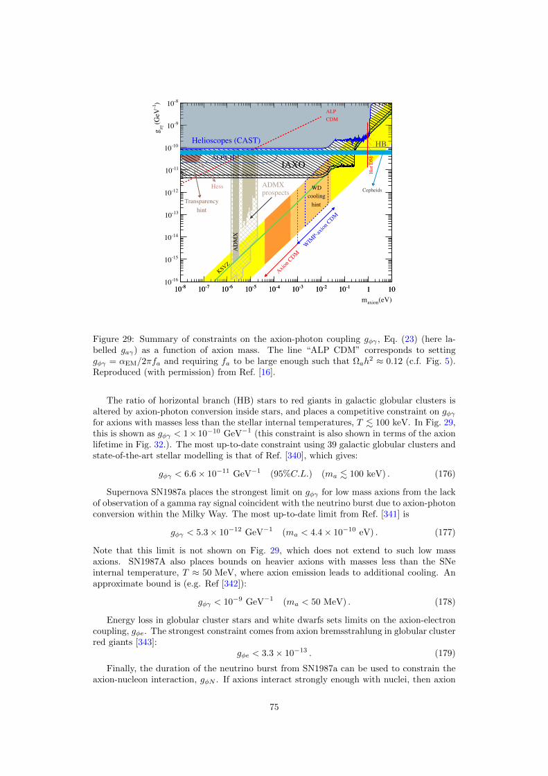
(eV)axionm

-810 -710 -610 -510 -410 -310 -210 -110 1 10

)-1

(GeV

γag

-1610

-1510

-1410

-1310

-1210

-1110

-1010

-910

-810

Hot

DM

Helioscopes (CAST)

IAXO

HB

KSVZAxio

n CDM

WIM

P-axion

CDM

AD

MX

ALPS-II

ALPCDM

CepheidsADMXprospects

Transparencyhint

Hess WDcooling

hint

-810 -710 -610 -510 -410 -310 -210 -110 1 10

Figure 29: Summary of constraints on the axion-photon coupling gφγ , Eq. (23) (here la-belled gaγ) as a function of axion mass. The line “ALP CDM” corresponds to settinggφγ = αEM/2πfa and requiring fa to be large enough such that Ωah

2 ≈ 0.12 (c.f. Fig. 5).Reproduced (with permission) from Ref. [16].

The ratio of horizontal branch (HB) stars to red giants in galactic globular clusters isaltered by axion-photon conversion inside stars, and places a competitive constraint on gφγfor axions with masses less than the stellar internal temperatures, T . 100 keV. In Fig. 29,this is shown as gφγ < 1×10−10 GeV−1 (this constraint is also shown in terms of the axionlifetime in Fig. 32.). The most up-to-date constraint using 39 galactic globular clusters andstate-of-the-art stellar modelling is that of Ref. [340], which gives:

gφγ < 6.6× 10−11 GeV−1 (95%C.L.) (ma . 100 keV) . (176)

Supernova SN1987a places the strongest limit on gφγ for low mass axions from the lackof observation of a gamma ray signal coincident with the neutrino burst due to axion-photonconversion within the Milky Way. The most up-to-date limit from Ref. [341] is

gφγ < 5.3× 10−12 GeV−1 (ma < 4.4× 10−10 eV) . (177)

Note that this limit is not shown on Fig. 29, which does not extend to such low massaxions. SN1987A also places bounds on heavier axions with masses less than the SNeinternal temperature, T ≈ 50 MeV, where axion emission leads to additional cooling. Anapproximate bound is (e.g. Ref [342]):

gφγ < 10−9 GeV−1 (ma < 50 MeV) . (178)

Energy loss in globular cluster stars and white dwarfs sets limits on the axion-electroncoupling, gφe. The strongest constraint comes from axion bremsstrahlung in globular clusterred giants [343]:

gφe < 3.3× 10−13 . (179)

Finally, the duration of the neutrino burst from SN1987a can be used to constrain theaxion-nucleon interaction, gφN . If axions interact strongly enough with nuclei, then axion

75

emission via nuclear bremsstrahlung, N +N → N +N + φ, is a more efficient energy-losschannel than neutrino emission, shortening the observed neutrino burst [344]. The theo-retical calculation of supernova energy loss involves many uncertainties, but approximatebounds can be obtained. For a KSVZ type axion with no tree-level fermion couplings thebound is (see Ref. [10] for discussion)

fa & 4× 108 GeV (KSVZ) . (180)

9.2 “Light Shining Through a Wall”

LSW is based on a very simple idea: shine a laser beam at a wall; apply a magnetic field sothat it converts into axions, which travel freely through the wall; on the other side of thewall apply another magnetic field to convert the axions back to observable photons (for areview, see Ref. [13]). Just like the stellar astrophysics limits, this is direct axion productionand applies regardless of whether the axion is DM.

The conversion probability, P (γ → φ), for photons of energy ω into axions in thepresence of a coherent magnetic field, B, of length L is

P (γ → φ) = 4g2φγB

2ω2

m4a

sin2

(m2aL

4ω

). (181)

The conversion probability can also be affected by using a medium with a refractive indexnr 6= 1, and by use of resonant cavities to enhance conversion and reconversion on eitherside of the wall.

The constraints from current LSW experiments are not particularly strong compared toastrophysical constraints, and do not appear on the scale of Fig. 29. The strongest boundscome from the Any Light Particle Search (ALPS) experiment [345] and are roughly

gφγ . 7× 10−8 GeV−1 (ma . 10−3 eV) . (182)

The planned experiment ALPS-II [346] will improve these limits by more than three ordersof magnitude, sensitive to gφγ ∼ 2 × 10−11 GeV−1 over a similar range of masses. Theprojected reach is shown in Fig. 29 and will be competitive with astrophysical and helioscopelimits discussed in Sec. 9.1.

9.3 Vacuum Birefringence and Dichroism

In the presence of a magnetic field, the Primakoff interaction between axions and photonsallows for the vacuum to become birefringent and dichroic [333]. These effects cause thepolarization plane of linearly polarized light to be rotated as it propagates. With no externalmagnetic field, we simply have birefringence (rotation with no absorption, we consider thiseffect in a cosmological context in Section 9.9), while in the presence of a magnetic field,there is absorption of one polarization state, i.e. dichroism. The amplitude of the dichroismis given by [347]

ε = sin 2θ

(BLgφγ

4

)2 [sin(m2

aL/4ω)

m2aL/4ω

]2

, (183)

where θ is the angle between the magnetic field, B, and the polarization direction, L isthe length of the magnetic region, and ω is the photon energy. The effect can be enhancedin a Fabrey-Perot cavity by increasing the number of passes the light makes in the cavity.Measuring the dichroism of the vacuum in the presence of a B-field can thus be used toplace constraints on the existence of axions possessing the two-photon coupling.

Using this technique, in 2006 PVLAS reported evidence for a polarization rotation inthe presence in a B ≈ 5 T field of α = (3.9±0.5)×10−12 rad/pass (3σ uncertainties). Thiswas interpreted as evidence for an axion with ma ≈ 1 meV and gφγ ≈ 10−5 GeV−1 [347].

76

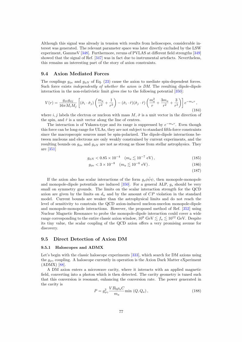
Although this signal was already in tension with results from helioscopes, considerable in-terest was generated. The relevant parameter space was later directly excluded by the LSWexperiment, GammeV [348]. Furthermore, reruns of PVLAS at different field strengths [349]showed that the signal of Ref. [347] was in fact due to instrumental artefacts. Nevertheless,this remains an interesting part of the story of axion constraints.

9.4 Axion Mediated Forces

The couplings gφe and gφN of Eq. (23) cause the axion to mediate spin-dependent forces.Such force exists independently of whether the axion is DM. The resulting dipole-dipoleinteraction in the non-relativistic limit gives rise to the following potential [350]:

V (r) =gφigφj

16πMiMj

[(σi · σj)

(ma

r2+

1

r3

)− (σi · r)(σj · r)

(m2a

r+

3ma

r2+

3

r3

)]e−mar ,

(184)where i, j labels the electron or nucleon with mass M , σ is a unit vector in the direction ofthe spin, and r is a unit vector along the line of centres.

The interaction is of Yukawa-type and its range is suppressed by e−mar. Even thoughthis force can be long-range for ULAs, they are not subject to standard fifth-force constraintssince the macropscopic sources must be spin-polarized. The dipole-dipole interactions be-tween nucleons and electrons are only weakly constrained by current experiments, and theresulting bounds on gφe and gφN are not as strong as those from stellar astrophysics. Theyare [351]

gφN < 0.85× 10−4 (ma . 10−7 eV) , (185)

gφe < 3× 10−8 (ma . 10−6 eV) . (186)

(187)

If the axion also has scalar interactions of the form gsφψψ, then monopole-monopoleand monopole-dipole potentials are induced [350]. For a general ALP, gs should be verysmall on symmetry grounds. The limits on the scalar interaction strength for the QCDaxion are given by the limits on dn and by the amount of CP violation in the standardmodel. Current bounds are weaker than the astrophysical limits and do not reach thelevel of sensitivity to constrain the QCD axion-induced nucleon-nucelon monopole-dipoleand monopole-monopole interactions. However, the proposed method of Ref. [352] usingNuclear Magnetic Resonance to probe the monopole-dipole interaction could cover a widerange corresponding to the entire classic axion window, 109 GeV . fa . 1012 GeV. Despiteits tiny value, the scalar coupling of the QCD axion offers a very promising avenue fordiscovery.

9.5 Direct Detection of Axion DM

9.5.1 Haloscopes and ADMX

Let’s begin with the classic haloscope experiments [333], which search for DM axions usingthe gφγ coupling. A haloscope currently in operation is the Axion Dark Matter eXperiment(ADMX) [88].

A DM axion enters a microwave cavity, where it interacts with an applied magneticfield, converting into a photon which is then detected. The cavity geometry is tuned suchthat this conversion is resonant, enhancing the conversion rate. The power generated inthe cavity is

P = g2φγ

V B0ρaC

mamin (Q,Qa) , (188)

77

Gray Rybka - PATRAS 2014, CERN July 2014 27/27

Conclusions

RF Cavities(ADMX)

Open Resonators?

Periodic Dielectrics?LC Circuits?

The entire classical axion window is within our reach

Not pictured: NMR, Dish Antenna, Tubes, future helioscopes, other ideas that may be presented or developed at this conference

Figure 30: Future reach of axion DM direct detection experiments using the two-photoncoupling. The classic window of the QCD axion can be completely covered. Reproduced,with permission, from “Resonant Dark Matter Detectors Beyond 10 GHz,” Gray Rybka,PATRAS10 (2014).

where ρa is the local DM density in axions, V is the cavity volume, B0 is the appliedmagnetic field strength, Q is the quality factor of the cavity, Qa is the ratio of the haloaxion energy to energy spread, and C is a mode dependent form factor for the cavity. Forapproximate ADMX parameters V = 500 L, B0 = 7 T, Q = 105, in the classic QCD axionwindow with fa ≈ 1012 GeV, the power is P ≈ 10−21 W.

Since ADMX is a DM detector, it also relies on ρa being large, and quoted constraintsassume that axions in its sensitivity range compose all the DM. Because of the resonanttuning required, ADMX is very precise, but is only able to probe a narrow range in the mass-coupling plane (see Fig. 29). ADMX is sensitive to axions with ma ≈ 10−6 eV. Currentconstraints exclude ALPs of this mass more strongly coupled to photons than the QCDaxion. In the near future ADMX will able to probe most of the model space (KSVZ andDFSZ) for the QCD axion with 10−6 eV . ma . 10−5 eV, i.e. fa ∼ 1012 GeV.

Other upgrades and new proposals for axion DM direct detection experiments in theclassic QCD axion window using the two-photon coupling include the use of open res-onators (the ORPHEUS experiment) [353], LC-circuits [354] and broadband searches withSQUIDs [355]. Projections for some of these techniques are shown in Fig. 30, and couldcover the mass range 10−8 eV . ma . 10−2 eV of the QCD axion.

9.5.2 Nuclear Magnetic Resonance and CASPEr

The Cosmic Axion Spin Precession Experiment (CASPEr) [235], comes in two varieties.Both strategies are novel, as they do not rely on the “standard” two-photon coupling. EachCASPEr experiment uses the property that the axion couplings to nucleons are spin depen-dent. The interactions can be detected by spin-polarizing a sample in an applied magneticfield, and searching for spin-precession using nuclear magnetic resonance techniques. Theinduced magnetization is resonant at the Larmour frequency of the applied magnetic field,2µmBext = ma (where µm is the nuclear magnetic dipole moment) and is detected using aSQUID magnetometer. For reasons that will become apparent, we refer to the two distinct

78

ADMX QCD Axion

SN 1987A

Static EDM

10!14 10!12 10!10 10!8 10!6 10!4 10!2 100

10!20

10!15

10!10

10!5

102 104 106 108 1010 1012 1014

mass !eV"

g d!GeV

!2 "

frequency !Hz"

SN 1987A

New Force

QCD Axion

ALP DM ADMX

10!14 10!12 10!10 10!8 10!6 10!4 10!2 100

10!20

10!18

10!16

10!14

10!12

10!10

10!8

10!6

10!4

102 104 106 108 1010 1012 1014

mass !eV"

g aNN!GeV

!1 "

frequency !Hz"

Figure 31: Sensitivity of the CASPEr experiments, assuming the DM is contained exclu-sively in a single ALP. CASPEr is a resonant experiment and sensitivity assumes a 3 yearoperation of scanning. Left Panel: CASPEr-Electric and the nucleon EDM coupling. Or-ange shaded: phase 1. Red shaded: phase 2. Dashed red: magnetometer noise limit inphase 2. Right Panel: CASPEr-Wind and the axial nucleon moment (note their gN is ourgN ). Red: Xe sample. Blue: 3He sample. Dashed lines: magnetization noise limits. Re-produced (with permission) from Refs. [235, 47]. Copyright (2014,2013) by The AmericanPhysical Society.

experiments as “CASPEr-Electric” [235] and “CASPEr-Wind” [47]. Just like with ADMX,CASPEr is a DM detector and the sensitivity to axions scales with the DM abundance.CASPEr has not yet been constructed, and we discuss projected sensitivities.

CASPEr-Electric exploits the axion coupling to (φ/fa)TrGG, which gives rise to theEDM coupling, gd. CASPEr-Electric thus explores the defining property of the QCD axion.The dipole moment induced by an axion is dn = gdφ. Recall that the QCD axion solves thestrong-CP problem by setting the time-average of the nucleon EDM to zero, as requiredby experiments constraining the static EDM [20]. The same oscillations in the axion fieldthat allow it to function as a DM candidate, however, lead to EDM oscillations, dn ∼10−16(φ/fa) cos(mat) e cm, where φ is the local value of the axion field amplitude. CASPEr-Electric applies an electric field to a spin-polarized sample and detects the precession of thenuclear spins about the ~E field axis caused by the non-zero EDM.

The projected sensitivity of CASPEr-Electric is shown in Fig. 31, Left Panel. In phase2 CASPEr-Electric will be able to detect the QCD axion for fa & 1016 GeV, with ultimatelimits from magnetization noise able to reach fa & 3× 1013 GeV. CASPEr-Electric is thushighly complementary to ADMX and astrophysical bounds.

CASPEr-Wind exploits the axion coupling to the axial nuclear current, gφN , and theinduced spin-dependent force. As the earth moves relative to the DM halo of our galaxy, sowe experience a “DM wind” of axions. The effective coupling in the nucleon Hamiltonianis HN ⊃ gφNmaφ cos(mat)~v ·~σ, where ~σ is the nuclear spin, and ~v is the DM wind velocity.The spin-dependent force creates a torque around the direction of the DM wind and leadsto spin precession of nuclei without the need for an applied electric field. CASPEr-Wind isthus somewhat simpler to implement than CASPEr-Electric.

The projected sensitivity of CASPEr-Wind is shown in Fig. 31, Right Panel. WhileCASPEr-Wind is not sensitive to the QCD axion (except in the noise-limited regime), itis sensitive to the ULA model of Ref. [46], and is complementary to cosmological axionsearches.

79

9.6 Heavy Axions and Axion Decays

In this section we consider constraints on axions with masses ma 1 eV. Note that theconstraints summarised in Fig. 29 (and much of the phenomenology discussed elsewhere inthis review) typically do not apply to such high masses, as they rely on the coherence ofthe axion field. The bounds from stellar astrophysics in Section 9.1 can apply for ma aslarge as 1 keV. We consider primarily the astrophysical and cosmological consequences ofaxion decay, but mention some other constraints in passing.

Consider the axion-photon coupling, gφγ , defined in Eq. (23), which we recall has mass-dimension −1, and is in general a free parameter for ALP models, with approximate scale1/fa. This coupling allows axions to decay into two photons, with a lifetime:

τφγ =64π

m3ag

2φγ

≈ 130 s

(GeV

ma

)3(10−12 GeV−1

gφγ

)2

. (189)

Consider the KSVZ axion, with the photon coupling fixed by Eq. (27). Taking the age ofthe Universe to be τuniv. ≈ 1010 years we find that the QCD axion is stable on the lifetimeof the Universe for fa & 1.9× 106 GeV. Thus, the QCD in the allowed range of fa is stableon the lifetime of the Universe, and hence is a DM candidate.

ALPs, on the other hand, may decay on much shorter time scales. The coupling of ALPsis in general proportional to the mass, since couplings go as 1/fa and ma = Λ2

a/fa. Thusheavier ALPs can be unstable on cosmological timescales and will decay to standard modelparticles (or light dark sector particles). The decay of such a population of ALPs injectsadditional relativistic energy density into the Universe, which is constrained by a number ofprobes. We will closely follow the recent compilation of constraints in Ref. [356], as shownin Fig. 32. Some early constraints on ALPs from decays can be found in Refs. [342, 357],while further reading can be found in Ref. [358] (for general physics and consequences ofdecaying particles, see Ref. [359]).

The presence and later decay of ALPs in the early Universe can change the effectivenumber of relativistic species, Neff (Eq. 44), and the baryon-to-photon ratio, ηb ≡ nb/nγ ,at different times in cosmological history. A lower value of NCMB

eff affects the CMB powerspectrum, as discussed in Section 3.3.1. The baryon ratio at the CMB is well measured,fixind ηCMB

b = 2.74 × 10−8Ωbh2. The photon energy density is also fixed by the equally

well measured TCMB. Therefore ALP decays can actually reduce Neff and increase ηb. AnALP decaying between BBN and the CMB reduces NCMB

eff if the decay occurs after neutrinodecoupling, by heating of the plasma.51 Decay before BBN also reduces NBBN

eff . On theother hand, if the ALPs are themselves relativistic at BBN, NBBN

eff is increased. ALP decaybetween BBN and the CMB leads to a relative increase ηBBN

b compared to ηCMBb .

Changes of the expansion rate , via Neff , and baryon abundance during BBN affect thelight element abundances. The standard model predictions of the BBN light element abun-dances are extremely well verified (with the famous exception of Lithium): see Refs. [42, 360]for reviews. The helium abundance, Yp and the deuterium-to-hydrogen ratio, D/H, placestrong constraints on ALPs, both from decays and from the contribution of thermally pro-duced axions with ma . 1 MeV to the radiation density at BBN.

Energy injections at different epochs can also change the shape of the CMB frequencypower spectrum, such that it is no longer a perfect black body. Such effects are knownas CMB spectral distortions, and are strongly constrained by the COBE-FIRAS measure-ments (for a review, see Ref. [228]). Early decays of axions heat the plasma leading todistortions of “µ-type” (chemical potential) for decays between 105 . z . 106, or “y-type”(Compton scattering) for decays between 1100 . z . 105. These effects are computed ine.g. Refs. [356, 358, 357].

51It is interesting to note the opposite effects of different ALPs on Neff : decay of a heavy particle to anALP leads to an increase, while decay of a heavy ALP to photons leads to a decrease. The effects of lightand heavy ALPs and moduli could conspire to hide them from our view.

80

3 4 5 6 7 8 9log10(mφ [eV])

4

2

0

2

4

6

log

10(τ φγ[s

ec])

HB Stars

CMB Anisotropies

D/H

Collider

Beam Dump

SN1987A

CMB Spectral Distortions

Yp

DFSZ-EN2

KSVZ

ν dec

BBN start

BBN end

Figure 32: Constraints on heavy ALPs from decays, in the mass-lifetime plane. The axionmass is here labelled mφ. The CMB, D/H, and Yp regions are excluded at 3σ, the Colliderand Beam Dump regions are excluded at 2σ, and the SN1987a and HB Stars regions areless formal. Reproduced (with permission) from Ref. [356].

In the life-time range of relevance to cosmological axion decays, the axion-photoncoupling also has collider signatures, allowing, for example, single-photon final states inelectron-positron colliders. The constraint from LEP [361, 362, 363] is [35]

gφγ < 4.5× 10−4 GeV−1 (LEP: ma . GeV) . (190)

In fact, a stronger bound due to the single photon final state was derived much earlier,using ASP data [364] in Ref. [342]: gφγ ≤ 5.5×10−4 GeV−1 for ma 29 GeV. Anomalousdecays of heavy quark states lead to similar bounds.

The summary of these constraints is shown in Fig. 32. The DFSZ and KSVZ axionmodels are excluded for ma in the keV to MeV range, as are most ALPs with

1 keV .ma . 1 GeV , (191)

10−4 s .τφγ . 106 s . (192)

There is an open window for short-lived, τφγ < 0.01 s, heavy, ma & 1 GeV, ALPs thatdecay early enough and are sufficiently non-relativistic at BBN to not alter the light elementabundances.

9.7 Axion Dark Radiation

We discussed in Section 3.3.1 how a population of relativistic axions can be created by decayof a modulus. The CMB power spectrum and other cosmological observables constrain thesimplest consequence of this: the relativistic axion energy density, parameterized by ∆Neff .This population of axions, if coupled to the standard model, can also be probed by axionscattering.

81

3 4 5 6 7 8

8.5

9

9.5

Log10!mΦ"2 GeV#

Log 10!f a"G

eV#

BBN bounds on fa

Figure 33: Constraints on axion DR from the primordial helium abundance [365]. Thefermion interaction is taken to have strength cf = 1, and here mφ is the modulus mass.Final states to bb (solid), cc (dashed) and ss (dot-dashed) are considered, with varyingamounts of DR, ∆Neff = 0.1, 0.5, 1 (green, black, red; corrected labelling from typo inoriginal). Areas below curves are excluded. Reproduced (with permission) from Ref. [108].

If the modulus decay that produced the axion DR also reheats the Universe, then theaxion energy is E ∼ mσ ∼ Tγ

√Mpl/mσ Tγ . Because the energy is much higher than

the plasma temperature, this gives access to processes that are otherwise kinematically for-bidden. This leads to interesting constraints and phenomenology despite the fa-suppressedaxion couplings. Ref. [108] discussed the phenomenology in detail.

An axion-fermion coupling of the form Lf = cfmfφψγ5ψ/fa (this form can be obtained

from the axial current interaction in Eq. 23 by use of the equations of motion) allows forproduction of heavy fermions via the process a + γ → f + f . The secondary decay ofthe fermions can alter the proton to neutron ratio during BBN, and thus the primordialhelium abundance. Each axion scattering process can be mapped onto an “effective decayprocess” [108] for which constraints can readily be found in the literature (e.g. Ref. [365]).The constraints are shown in Fig. 33. Taking cf = 1, BBN constraints rule out values offa . 109 GeV over a wide range of modulus masses.

Axion DR also has a flux at Earth and, if the axion-photon coupling is non-vanishing,could be detected by helioscopes like CAST. The axion DR flux is distinct from the solar fluxin two important ways: firstly, because of its cosmological origin, it is isotropic; secondly,the DR flux is not suppressed by as many powers of gφγ , due to the different productionmechanism compared to solar axions. Taking gφγ ∼ f−1

a , the DR signal in a heliscope is thussuppressed as only f−2

a , compared to the f−4a suppression for solar axions. For a modulus

mass of mσ = 5 × 106 GeV and ∆Neff ≈ 0.6 the flux is Φa ≈ 1.09 × 106 cm−2s−1 [108],which is of order the solar QCD axion flux for fa = 1010 GeV. The DR background in thismodel is thus in reach of IAXO. For these same parameters, the energy spectrum peaks inthe keV range, and has a form characteristic of the axion DR background from modulusdecay.

82

-18 -16 -14 -12 -10

log[mþ [eV]]

gh B

2i

10-10GeV

ánG]

[10

-4

10-2

10-6

0

1=2

-1FIRAS bound

PIXIE/PRISM

= 3! = T0

! = 10T0

= 4! = T0

Figure 34: Constraints on ULAs from CMB spectral distortions from FIRAS, and projectedfor PIXIE/PRISM. The axion mass is labelled mφ in this plot. The dark band shows masseswhere multiple resonant conversions effectively exclude such axions entirely, for gφγ 6= 0.Reproduced (with permission) from Ref. [371]. Copyright (2013) by The American PhysicalSociety.

9.8 Axions and Astrophysical Magnetic Fields

Let’s further consider the Primakoff process, but now for the case of ULAs in the presence ofastrophysical magnetic fields. Gamma rays from blazars suggest that the cosmic backgroundfield exceeds B ∼ 10−16 G in large voids [366, 367], while it could be large as nG, with Mpccoherence length. Larger magnetic fields are present in clusters of galaxies, with strengthB ∼ µG and coherence length of order kpc.

9.8.1 CMB Spectral Distortions

In the presence of a background magnetic field axion photon mixing occurs and, just likein the case of massive neutrinos, propagation and interaction eigenstates are not the same.Furthermore, plasma effects lead to an effective photon mass:

m2γ = ω2

p(z)− 2ω2(nH − 1) , (193)

where ω is the photon frequency, and the refractive index of neutral hydrogen is nH . Theplasma frequency, ωp, depends on the free electron density, and is thus a function of redshiftdetermined by recombination and reionization. At ω = TCMB the photon plasma mass atz = 0 is mγ ∼ 10−14 eV. Resonant axion-photon conversion occurs when mγ = ma.Since for high frequency photons m2

γ passes through zero, resonant conversion can occurfor arbitrarily low axion mass, and can occur multiple times as m2

γ changes sign.The frequency dependence of the resonant conversion epoch leads to a spectral distor-

tion [368]. COBE-FIRAS [369, 370] measured the CMB to be a black body to high precision.This constrains the resonant conversion probability, which in turn leads to a constraint onthe product gφγB0, where B0 is the spatially averaged magnetic field strength today.

The constraints have been addressed in detail in Refs. [372, 371]. Fig. 34 shows the con-straints on ULAs from FIRAS, and projected constraints from a PIXIE [373]/PRISM [374]-like mission. Multiple resonant conversions occur for 10−14 eV . ma . 10−12 eV, effec-tively excluding any gφγ 6= 0 for this mass range. While constraints are only on the product

83

gφγB0, they are stronger than the product of current upper limits on gφγ and B0 individu-ally.

9.8.2 X-ray Production

As discussed a number of times, axion DR can be produced by the decay of a modulus, andthe axion DR energy today is E0 ∼ TCMB

√Mpl/mσ. For a modulus mass mσ ∼ 106 GeV

(suggested by string theory solutions to the EW hierarchy problem) this gives rise to acosmic axion background (CAB) with energy E ∼ 0.1 - 1 keV. The energy density in theCAB is

ρCAB = 1.6× 1060 erg Mpc−3

(∆Neff

0.57

), (194)

Conversion of the CAB to photons in the presence of magnetic fields leads to productionof X-rays.

Clusters of galaxies are permeated by magnetic fields with B ∼ µG and coherencelengths L ∼ kpc. Axion-photon conversion in this environment is predicted to lead toexcess X-ray emission from clusters [108, 375]. The X-ray luminosity of a typical Mpcsized cluster is Lcluster ∼ 1044 erg s−1. The excess soft X-ray luminosity in Coma is 1.6 ×1042 erg s−1 [376], which could plausibly be explained with an axion-photon coupling gφγ ∼10−14 GeV−1 [375], depending on the axion mass and the photon plasma mass in the intra-cluster medium. This emission has fixed redshift scalings, since the CAB is cosmological inorigin. It is also predicted to correlate with cluster magnetic fields, unlike an annihilatingDM signal.

Ref. [377] considered X-ray production within galactic magnetic fields. For the strengthof coupling required to explain the soft X-ray excess in Coma, conversion within the MilkyWay is negligible. Star burst galaxies, with larger magnetic fields, may produce an ob-servable signal, in particular if the inhomogeneous free electron density is accounted for inmodelling the emission.

Conversion in cosmological magnetic fields could contribute to an unresolved cosmicX-ray background. This is essentially the inverse of the spectral distortion effect discussedin the previous subsection, with a different energy spectrum. A diffuse cosmic X-ray back-ground in the keV energy range is observed [378], with diffuse intensity that could beexplained by the CAB with gφγ ∼ 10−13 GeV−1, assuming nG strength cosmological mag-netic fields [375]. From Fig. 34 we see that this explanation for the X-ray background willin addition produce a CMB spectral distortion close to the FIRAS bound, and observablewith PIXIE/PRISM.

9.9 Cosmological Birefringence

CMB polarization comes in E-modes and B-modes. E-modes are generated from tempera-ture fluctuations at last scattering by the quadrupole anisotropy, and the E spectrum can bepredicted from the measurement of the adiabatic temperature fluctuations. B-modes canbe generated in three ways: primordially, by tensor fluctuations with relative amplituderT ; by gravitational lensing along the line of sight; and finally by the birefringent effect,rotating of E into B.

In the presence of the axion-photon coupling in Eq. (23), the fields satisfying free wave

equations are ~D = ~E +gφγ2 φ~B and ~H = ~B − gφγ

2 φ~E [380] (note ~E and ~B are the fields ofelectromagnetism, and are not the same as E and B mode polarization). Therefore, if theaxion field φ varies in time or space it can cause rotation of the plane of polarization of theCMB [381]:

∆β =gφγ2

∫dτφ′ , (195)

where it is reminded that τ is conformal time, and primes denote derivatives with respectto this. The integral is performed along the line of sight from the surface of last scattering

84

Figure 35: CMB B-mode power from birefringence caused by ULAs coupled to magneticfields with (HIgφγ)2 ≈ 0.17 (red, solid). The large angle signal can mimic tensor modeswith r ∼ 0.1 (blue, short dashed), while the small angle signal contains distinctive BAOfrom the E-modes (green, dot-dashed) and, for this choice of parameters, dominates overlensing power (cyan, long dashed). Reproduced (with permission) from Ref. [379] (wherethe data are described). Copyright (2009) by The American Physical Society.

85

at zdec to today. When the axion is oscillating, the integral vanishes. Therefore, significantrotation only occurs for ULAs that begin oscillations after photon decoupling. Using zdec =1020, Ωm = 0.31, ΩΛ = 0.69, h = 0.67, we find that ULAs with a mass ma . 3Hdec =1× 10−28 eV can cause significant cosmological birefringence.

The uniform misalignment of ULAs in the broken PQ scenario (see Section 3.2.2) leads toa uniform rotation of the plane of CMB polarization. Such a uniform rotation is constrainedto be |∆β| < 1.4×10−2 [382]. If we assume φ(τ0) = 0, this gives the approximate constraintφigφγ < 2.8×10−3. Taking gφγ ∼ αEMf

−1a , CMB polarization rotation imposes a constraint

on the (φi, fa) plane. For ULAs, and using Eq. (61) for aeq < aosc, the birefringenceconstraint is of order the constraint on the DM abundance from temperature anisotropies(Fig. 15, right panel), assuming fa < Mpl and ma . 1 × 10−28 eV (excluding also thelightest DE like axions where φ(τ0) 6= 0). Thus, if a sub-dominant population of such ULAsis detected in LSS in future, e.g. by Euclid (Fig. 14), then this may well be accompaniedby birefringence in the CMB.

Anisotropies in the axion field cause anisotropic rotation. This leads to generation ofBB anisotropy power from EE, and thus EB cross-correlations, and can be significantlysourced by ULA isocurvature pertrubations: see e.g. Refs. [383, 382, 379, 384, 385]. Theresulting CMB power spectra are shown in Fig. 35. The amplitude of the power spectrumscales as (HIgφγ)2. This effect is particularly interesting as it can generate B-modes thatdominate over those produced by tensor perturbations. This could source large angle B-mode power in low-scale inflation if HIgφγ ∼ 0.1. Since the power is generated from theE-modes, there is also oscillating, large amplitude, small-angle B-power in this scenario.This would be present even after de-lensing and is distinct from the tensor mode power,which falls rapidly on small angular scales.

The most recent constraints on anisotropic birefringence come from the B-mode powerand 4-point function measured by Polarbear [386]. These constraints are consistent withzero signal.

10 Concluding Remarks

In this review we have presented the vast cornucopia of axion physics. We have consideredthe motivations and models for axions coming from particle physics and string theory. Wehave seen how axions can be produced in the early Universe by a variety of mechanisms.Axions can play important roles in all of the unsolved mysteries of cosmology: inflation,dark matter, and dark energy. They also lead to novel phenomena, such as fuzzy darkmatter, and dark radiation. Axion couplings to the standard model are fixed by symmetryconsiderations, and can be computed in specific models. We studied the tailored direct andindirect searches for axions, which are quite different to more “standard” searches for newparticle physics.

I hope, dear reader, that you have come away from this review with a sense for thefascinating progress that has been made in axion physics over the last years and decades.I also hope that you can see the places on the horizon where new opportunities are arising.Let me briefly reiterate some of these:

• The dark sector and large scale structure: Soon, large scale structure measurementswill reach the precision to test in detail aspects of standard neutrino physics, such asthe neutrino mass, and number of neutrinos. Axions share many degeneracies withthe neutrino sector. Misalignment-produced ULAs suppress structure formation oncluster scales; hot axions contribute to dark radiation either via thermal productionor via modulus decay. Improved measurements and studies of CMB polarization andgravitational lensing of galaxies could easily discover these effects at the same time astesting neutrino physics. Breaking degeneracies via multiple probes is an importantendeavour for both axion and neutrino physics.

86

• Axions with ma ∼ 10−22 eV and the CDM small-scale crises: The CDM small-scalecrises, if they are indeed crises, can be solved by ULAs. Observational and simulationtechniques on these scales are always improving, and axion physics must keep up.There are some simulations on the market, but the field has not been studied inanywhere near as much depth as competing models, such as WDM. The tantalizingprospect to see evidence for axions on these scales, in galactic dynamics and in theepoch of reionization, must not be overlooked, and much work is necessary to exploitthis opportunity.

• Progress in string theory model building and the axiverse: A large part of the mo-tivation to study axions comes from their apparent prevalence in string theory. Inprinciple, therefore, constraints on axions can be interpreted as constraints on stringtheory. There is already a large program of model building in this direction. The focushas largely been on inflation, but extensions to other parts of cosmology are slowlybeing made. This model building should also be done holistically, with emphasis onthe many different facets of axion physics that combine and provide the opportunityto make unique and verifiable predictions.

• Novel experiments for axion direct detection: Axion direct detection has, for manyyears, focused on the ~E · ~B coupling and the QCD axion. Recent years have seenan upsurge in interest in searching for the other possible axion couplings in terres-trial experiments. These searches are more generally applicable to ALPs, which mayonly possess a fraction of the couplings allowed by symmetry, for example havingno coupling to photons. All direct searches for axions provide vital information tocosmology, not least by limiting the decay constant in specific models, but also byallowing the possibility to actually identify the DM as axion-like by the form of itscouplings.

This summary is not the end. Axion physics is alive and well, and growing: long mayit be so.

Acknowledgments. This review was prepared in part for a lecture presented at the mini-workshop “Axion Theory and Searches” at IPhT CEA/Saclay. I would like to thank theorganisers of the workshop, Marco Cirelli, Bradley Kavanagh and Filippo Sala, for invitingme to lecture, and the other lecturers, Joerg Jaeckel and Pierre Sikivie, for stimulatingdiscussion. I thank all my collaborators on the work presented here: Brandon Bozek,Malcolm Fairbairn, Pedro Ferreira, Daniel Grin, Renee Hlozek, Robert Hogan, Luca Iliesiu,Edward Macaulay, Kavilan Moodley, Ana Pop, Joseph Silk, Hiroyuki Tashiro, MaximeTrebistch, Scott Watson and Rosemary Wyse. Special thanks to the authors of Refs. [74,328, 108, 16, 257, 278, 356, 379, 298, 235, 47, 300] for permission to reproduce their figures.I thank Jihn Kim and Maxim Pospelov for discussions on the particle theory of axions,Thomas Bachlechner for discussion on the weak gravity conjecture, Sacha Davidson fordiscussion of BEC’s, and Renee Hlozek and Cliff Burgess for reading parts of the manuscript.Finally, I thank the anonymous referee, whose comments helped greatly improve the breadthof this work. This work was supported at Perimeter Institute by the Government of Canadathrough Industry Canada and by the Province of Ontario through the Ministry of Researchand Innovation; and by a Royal Astronomical Society research fellowship, hosted at King’sCollege London.

A Theta Vacua of Gauge Theories

I will simply state some relevant results to give you a feel for this topic: see the won-derful book by Coleman, Ref. [18], for the gory details. I follow Coleman’s notation andnormalisation in this discussion.

87

Quantum theory depends on the Euclidean functional integral, with the path integralbeing dominated by field configurations of finite Euclidean action. These dominant contri-butions to the semi-classical approximation are known as instantons. The action for a gaugefield theory with gauge group G (for definiteness, take G = SU(N)) and gauge coupling gGin 4 flat Euclidean dimensions is

S =1

4g2G

∫d4x(Fµν , Fµν) (A1)

A field configuration of finite action must have F ∼ O(1/r3) as r → ∞ and so the gaugefield must be of the form

Aµ = g∂µg−1 +O(1/r2) , (A2)

for some gauge transformation g(x), which is a function mapping G to the variables ofEuclidean 4-space. In order not to alter the asymptotic baheviour in r we must have thatg(x) maps G to only the angular vairables. That is, the field configurations are definedup to a mapping of G to the space-time boundary, which in this case is topologically thethree-dimensional hypersphere, S3.

How many different mappings are there, and how can we classify them? Firstly, wecan always make a gauge transformation by some other element h, which is a continuousfunction, and continuously deform one into another. That means that all homotopoicallyequivalent mappings are equivalent field configurations.52 We now need to classify thehomotopically distinct mappings.

A theorem [387] states that we need only consider the SU(2) subgroups of our groupG. SU(2) is topologically S3, and so one such mapping is the trivial mapping

g(1)(x) = (x4 + i~x · ~σ)/r , (A3)

where σ1,2,3 are the Pauli matrices. It is then also possible to prove (Coleman does notprove it, and I certainly won’t) that all mappings from S3 to S3 are homotopic to a familyof mappings

g(ν)(x) = [g(1)(x)]ν , (A4)

where ν is an integer called the winding number. For the simple example of wrapping U(1)round a circle, this is easy to visualise, and ν labels the representations of U(1) as eiνθ,with θ the angle on S1.

Finally, it is possible to show that the winding number of a field configuration is givenby the integral

ν =1

32π2

∫d4x(F, F ) , (A5)

where F is the dual field strength as defined below Eq. (2). The winding number is a topo-logical invariant of the field configuration, providing a finite contribution to the Euclideanaction proportional to the integral of Eq. (2).

The winding number describes the boundary conditions of the gauge fields with ν = nin some state |n〉. The vacuum of the theory is given by a superposition of states

|θ〉 =∑n

einθ|n〉 . (A6)

such that

〈θ|e−HT |θ〉 ∝∫

[dA]e−Seiνθ . (A7)

52An important consequence of this is the fact that U(1) gauge theory has no instantons in 3+1 dimen-sions. U(1) is topologically the circle, S1, which, when wrapped around S3, can be continuously deformedto a single point: the trivial mapping.

88

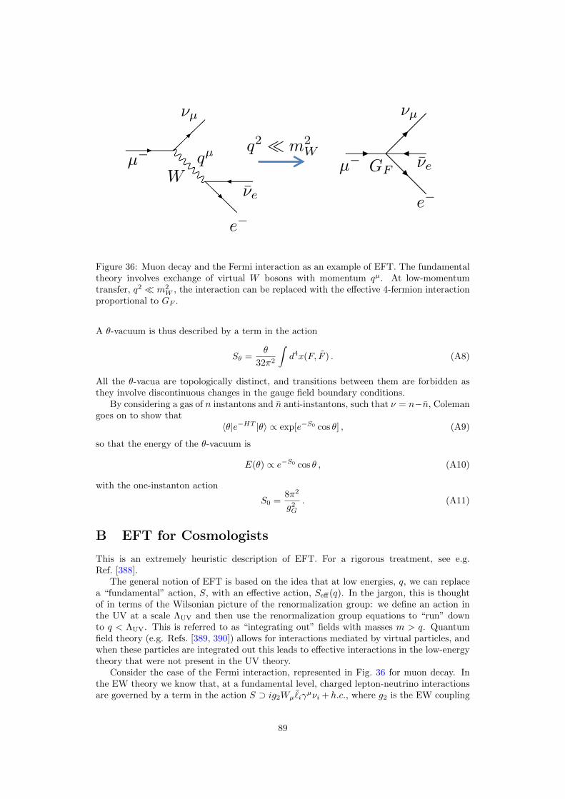
ee

Wqµ q2 m2

W

GF

e

eµµ

µ µ

Figure 36: Muon decay and the Fermi interaction as an example of EFT. The fundamentaltheory involves exchange of virtual W bosons with momentum qµ. At low-momentumtransfer, q2 m2

W , the interaction can be replaced with the effective 4-fermion interactionproportional to GF .

A θ-vacuum is thus described by a term in the action

Sθ =θ

32π2

∫d4x(F, F ) . (A8)

All the θ-vacua are topologically distinct, and transitions between them are forbidden asthey involve discontinuous changes in the gauge field boundary conditions.

By considering a gas of n instantons and n anti-instantons, such that ν = n−n, Colemangoes on to show that

〈θ|e−HT |θ〉 ∝ exp[e−S0 cos θ] , (A9)

so that the energy of the θ-vacuum is

E(θ) ∝ e−S0 cos θ , (A10)

with the one-instanton action

S0 =8π2

g2G

. (A11)

B EFT for Cosmologists

This is an extremely heuristic description of EFT. For a rigorous treatment, see e.g.Ref. [388].

The general notion of EFT is based on the idea that at low energies, q, we can replacea “fundamental” action, S, with an effective action, Seff(q). In the jargon, this is thoughtof in terms of the Wilsonian picture of the renormalization group: we define an action inthe UV at a scale ΛUV and then use the renormalization group equations to “run” downto q < ΛUV. This is referred to as “integrating out” fields with masses m > q. Quantumfield theory (e.g. Refs. [389, 390]) allows for interactions mediated by virtual particles, andwhen these particles are integrated out this leads to effective interactions in the low-energytheory that were not present in the UV theory.

Consider the case of the Fermi interaction, represented in Fig. 36 for muon decay. Inthe EW theory we know that, at a fundamental level, charged lepton-neutrino interactionsare governed by a term in the action S ⊃ ig2Wµ

¯iγµνi + h.c., where g2 is the EW coupling

89

qµ

g

g

g

g

1/faq2 m2

Q

Q

Q

Q

Figure 37: The colour anomaly in the KSVZ axion model. Heavy quarks, Q, run in a loopwith momentum qµ. At low-momentum transfer, q2 m2

Q, the interaction can be replaced

with the effective φGG/fa interaction.

constant, `i is the charged lepton field, νi its corresponding neutrino, and Wµ is a charged Wboson. This allows for W± particles to mediate muon decay (recall that a similar processinvolving quarks and the CKM matrix elements mediates nuclear β-decay, and was theoriginal use of the Fermi interaction). The exchanged 4-momentum is qµ, and the W -bosonpropagator is proportional to 1/(q2 +m2

W ), where mW = 80.4 GeV [42] is the mass of theW . At small momentum transfer, q2 m2

W (corresponding via the uncertainty principleto large distances) the propagator can be replaced by an effective 4-fermion interactionproportional to g2

2/m2W . Higher order interactions come suppressed by higher powers of

mW . In the low-energy EFT we replace the EW gauge invariant interaction with the Fermiinteraction using GF =

√2g2

2/8m2W . For muon decay, the low energy theory has a term in

the effective action Seff(q < mW ) ⊃ GF (eνe)(νµµ) + h.c.The situation with axions and the chiral anomaly is more complicated to compute,

but is easy to represent in pictures. The case of the KSVZ axion model is shown inFig. 37. The fundamental action contains Yukawa interactions between the axion andthe heavy quark fields, Q. The Q fields also interact with gluons. Virtual Q-particlesthen induce an effective axion-gluon interaction at loop-level. At low momentum transfer,q2 m2

Q, the heavy quarks can be integrated out and the effective action has a term

Seff(q < mQ) ⊃ φGG/32π2fa. This is the dominant term in the expansion in powers of1/mQ. It gives the largest contribution to the explicit breaking of U(1)PQ, and thus the

axion potential, and also generates the necessary GG interaction required for a solution tothe strong-CP problem. EFT can also be applied to light quarks after chiral symmetrybreaking. This gives rise to the second term in Eq. (25), which gives a contribution to theaxion-photon coupling from the colour anomaly.

C Friedmann Equations

Consider the line element for the flat Friedmann-Robertson-Walker (FRW) Universe:

ds2 = −dt2 + a(t)2d~x2 , (B1)

where a(t) is the cosmic scale factor. The scale factor obeys the Friedmann equations:

3H2M2pl = ρ ,

6(H +H2)M2pl = ρ+ 3P , (B2)

90

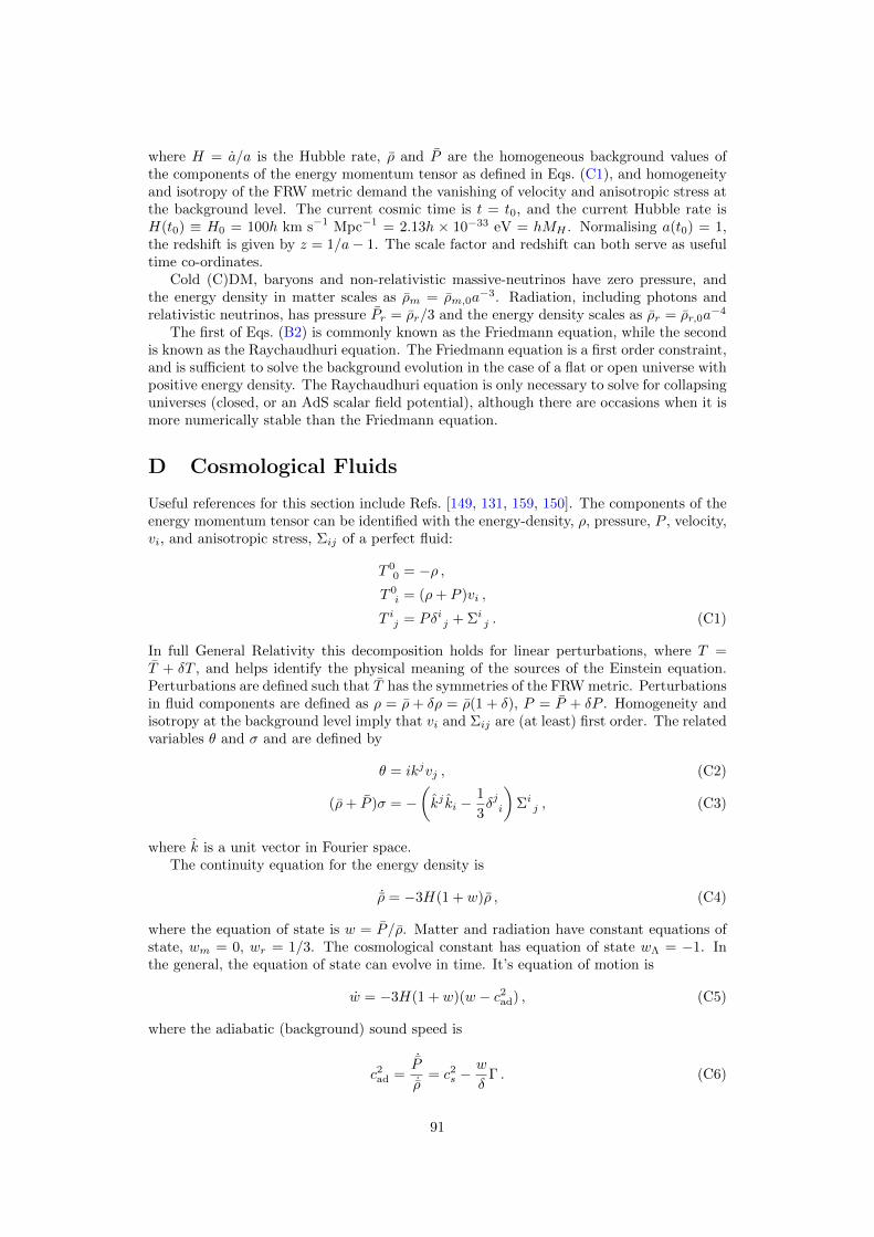
where H = a/a is the Hubble rate, ρ and P are the homogeneous background values ofthe components of the energy momentum tensor as defined in Eqs. (C1), and homogeneityand isotropy of the FRW metric demand the vanishing of velocity and anisotropic stress atthe background level. The current cosmic time is t = t0, and the current Hubble rate isH(t0) ≡ H0 = 100h km s−1 Mpc−1 = 2.13h × 10−33 eV = hMH . Normalising a(t0) = 1,the redshift is given by z = 1/a− 1. The scale factor and redshift can both serve as usefultime co-ordinates.

Cold (C)DM, baryons and non-relativistic massive-neutrinos have zero pressure, andthe energy density in matter scales as ρm = ρm,0a

−3. Radiation, including photons andrelativistic neutrinos, has pressure Pr = ρr/3 and the energy density scales as ρr = ρr,0a

−4

The first of Eqs. (B2) is commonly known as the Friedmann equation, while the secondis known as the Raychaudhuri equation. The Friedmann equation is a first order constraint,and is sufficient to solve the background evolution in the case of a flat or open universe withpositive energy density. The Raychaudhuri equation is only necessary to solve for collapsinguniverses (closed, or an AdS scalar field potential), although there are occasions when it ismore numerically stable than the Friedmann equation.

D Cosmological Fluids

Useful references for this section include Refs. [149, 131, 159, 150]. The components of theenergy momentum tensor can be identified with the energy-density, ρ, pressure, P , velocity,vi, and anisotropic stress, Σij of a perfect fluid:

T 00 = −ρ ,

T 0i = (ρ+ P )vi ,

T ij = Pδij + Σi j . (C1)

In full General Relativity this decomposition holds for linear perturbations, where T =T + δT , and helps identify the physical meaning of the sources of the Einstein equation.Perturbations are defined such that T has the symmetries of the FRW metric. Perturbationsin fluid components are defined as ρ = ρ + δρ = ρ(1 + δ), P = P + δP . Homogeneity andisotropy at the background level imply that vi and Σij are (at least) first order. The relatedvariables θ and σ and are defined by

θ = ikjvj , (C2)

(ρ+ P )σ = −(kj ki −

1

3δji

)Σi j , (C3)

where k is a unit vector in Fourier space.The continuity equation for the energy density is

˙ρ = −3H(1 + w)ρ , (C4)

where the equation of state is w = P /ρ. Matter and radiation have constant equations ofstate, wm = 0, wr = 1/3. The cosmological constant has equation of state wΛ = −1. Inthe general, the equation of state can evolve in time. It’s equation of motion is

w = −3H(1 + w)(w − c2ad) , (C5)

where the adiabatic (background) sound speed is

c2ad =˙P˙ρ

= c2s −w

δΓ . (C6)

91

The sound speed in fluctuations is

c2s =δP

δρ, (C7)

and Γ is the non-adiabatic pressure perturbation.It is important to note that definitions of “sound speed” are not universal, and that the

sound speed itself is not gauge invariant. I adopt the definitions above, and apply them inwhatever gauge we happen to be working in (synchronous or Newtonian). This is in keepingwith the treatment of Ref. [149], and is convenient and intuitive for standard cosmologicalperturbation theory as applied to the post-inflationary universe.

Some authors define the sound speed as the co-efficient in the equation of motion ofthe gauge invariant “Mukhanov-Sasaki” variable, ν. This is common in inflationary theory,and among relativists. For a scalar field, let’s denote this particular sound speed c2φ. One

can prove that c2φ = 1: i.e. it is the sound speed in the gauge in which δφ = 0 (flatscalar field slicing). The non-trivial growth and scalar field Jeans scale in this formulationcan be understood from the behaviour of the background (anti-)friction terms induced bygauge transformations from, e.g., the Newtonian gauge to the δφ = 0 gauge [163]. This isconsistent with the time-averaged effective sound-speed we employed in Section 4.4.3, andthe driven nature of Eqs. (74) and Eqs. (75) in the oscillating regime [159].

E Bayes Theorem and Priors

All cosmologists worth their salt are Bayesians. This happy state of affairs is forced upon usby the unavoidably one-shot nature of observing the cosmos. An introduction to Bayesianmethods in cosmology can be found in Ref. [391], with a more advanced specific treatmentin Ref. [392].

We are interested in the probability of our theory, specifed by a vector of parameters ~θ,given the data D: P (~θ|D). What we have access to is the likelihood, L, i.e. the probability

of the data given the theory: P (D|~θ) = L(D, ~θ). Bayes theorem relates these for us:

P (~θ|D) =P (D|~θ)P (~θ)

P (D); posterior =

likelihood × prior

evidence. (D1)

The probability of the theory, P (~θ), is the all-important prior. In an MCMC setting,the prior can be thought of as the distribution from which we draw sample theory curvesto compare to the data (although it can also be imposed later on top of uniform sampling).The probability of the data, P (D), can be computed as a normalization. It can often beignored, since we are interested in ratios of probabilities, although it is important for modelcomparison and Bayesian evidence.

The likelihood reflects our uncertainty on the data. A very simple assumption is toweight data points individually, and assume Gaussian errors, so that a model has a likelihoodas a product of Gaussians given by the distance of the theory curve from each data point.In many real-world examples, the likelihood is much more complicated. For example, thePlanck likelihood is discussed in Ref. [214].

The prior reflects our degree of belief in a model, and is often where physics can beput in. See Ref. [393] for an example in dark energy theory, and the formalism for treatinginformation gain over the prior in a Bayesian context.

An “uniformative” prior is the Jeffreys prior, which for most practical purposes is flatin log space. It is a suitable prior for unknown energy scales, for example the axion massand decay constant. The log-flat prior on axion mass is also physically motivated: instring theory the mass scales exponentially with some modulus, σ, of the compact space:ma,i ∝ e−cσi , where i labels the axion species. The moduli are expected to have a uniformdistribution in real space (since the scale is set by the compactification volume), leading

92

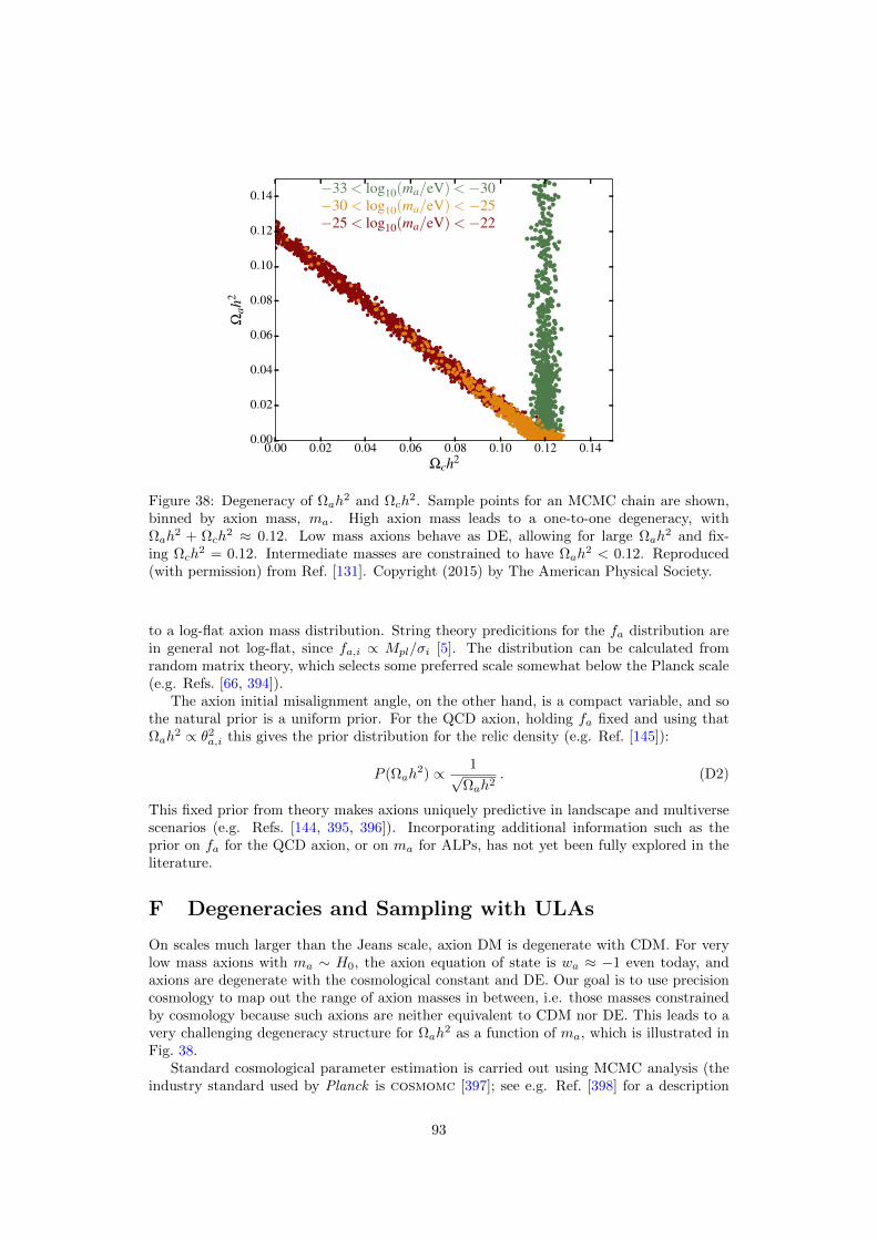
0.00 0.02 0.04 0.06 0.08 0.10 0.12 0.14!ch2

0.00

0.02

0.04

0.06

0.08

0.10

0.12

0.14

!ah

2

!33 < log10(ma/eV) < !30!30 < log10(ma/eV) < !25!25 < log10(ma/eV) < !22

Figure 38: Degeneracy of Ωah2 and Ωch

2. Sample points for an MCMC chain are shown,binned by axion mass, ma. High axion mass leads to a one-to-one degeneracy, withΩah

2 + Ωch2 ≈ 0.12. Low mass axions behave as DE, allowing for large Ωah

2 and fix-ing Ωch

2 = 0.12. Intermediate masses are constrained to have Ωah2 < 0.12. Reproduced

(with permission) from Ref. [131]. Copyright (2015) by The American Physical Society.

to a log-flat axion mass distribution. String theory predicitions for the fa distribution arein general not log-flat, since fa,i ∝ Mpl/σi [5]. The distribution can be calculated fromrandom matrix theory, which selects some preferred scale somewhat below the Planck scale(e.g. Refs. [66, 394]).

The axion initial misalignment angle, on the other hand, is a compact variable, and sothe natural prior is a uniform prior. For the QCD axion, holding fa fixed and using thatΩah

2 ∝ θ2a,i this gives the prior distribution for the relic density (e.g. Ref. [145]):

P (Ωah2) ∝ 1√

Ωah2. (D2)

This fixed prior from theory makes axions uniquely predictive in landscape and multiversescenarios (e.g. Refs. [144, 395, 396]). Incorporating additional information such as theprior on fa for the QCD axion, or on ma for ALPs, has not yet been fully explored in theliterature.

F Degeneracies and Sampling with ULAs

On scales much larger than the Jeans scale, axion DM is degenerate with CDM. For verylow mass axions with ma ∼ H0, the axion equation of state is wa ≈ −1 even today, andaxions are degenerate with the cosmological constant and DE. Our goal is to use precisioncosmology to map out the range of axion masses in between, i.e. those masses constrainedby cosmology because such axions are neither equivalent to CDM nor DE. This leads to avery challenging degeneracy structure for Ωah

2 as a function of ma, which is illustrated inFig. 38.

Standard cosmological parameter estimation is carried out using MCMC analysis (theindustry standard used by Planck is cosmomc [397]; see e.g. Ref. [398] for a description

93

of the methodology). The chain is begun at some location close to the maximum likeli-hood, and then randomly (and ergodically) explores this likelihood, with the density ofsamples reflecting the value of the likelihood. With infinite computing time, the processis guaranteed to explore the entire likelihood. Allowing for a wide prior on ma makes theconvergence of this process very slow, and the chain can get “stuck” in particular regions(modes) of the likelihood. For example, we might get stuck in a high-likelihood region withlarge ma, and Ωah

2 ≈ Ωch2. What we really want to know is the constraint on Ωah

2 atintermediate masses, and what the range of “intermediate” really is for a given observable.

Working around this bottleneck requires using different tools to estimate the likelihoodthan a standard “out-of-the-box” MCMC. The method employed in Ref. [131] used nestedsampling with multinest [225], an algorithm designed for multi-modal likelihoods, insteadof MCMC. However, it still proved prohibitively expensive to have enough sample points toachieve accurate limits on Ωah

2 across the full range of ma in the two dimensional (ma,Ωa)plane. A two-step procedure was used to overcome this. Three separate mass ranges ranindependently. A more coarse global chain was then ran, and the information from this wasused to importance-sample the individual chains together on the (ma,Ωa) plane.53

The procedure described above was able to deal with the degeneracies between CDM,DE and axions that occur for high and low ULA masses respectively. A separate issuethat has yet to be addressed fully is the degeneracy between ULAs and neutrinos at inter-mediate ULA mass. Cosmology is approaching the required precision to detect the effectsof∑mν = 0.06 eV, the minimum consistent with oscillation experiments. It is crucially

important to address all possible degeneracies so that a future detection can be consideredrobust. Ref. [171] used a grid-based likelihood, where convergence is not an issue, but onlyconstrained ma and mν independently. Grids scale poorly for large numbers of parameters,and are unsuitable for precision analysis. Ref. [172] performed a preliminary investigationusing a Fisher matrix formalism to perform forecasts. At the level of the study, degeneracieswere not too severe: the difference in behaviour between axions and neutrinos during theradiation era breaks the degeneracy in the effect on structure formation. However, Ref. [172]looked at individual ULA masses independently, and did not study the degeneracies as afunction of ULA mass. Including ULAs, CDM and neutrinos in a full parameter estimationpipeline will likely require further tricks like those described here to be employed whensampling the likelihood.

In general, when considering degeneracies, it is important to break the effects of axionDM up into two parts: effects on the background expansion, and effects on the perturba-tions. Axion cosmology coming purely from the misalignment production is a well definedmodel where all effects on the expansion rate, clustering and initial conditions come pack-aged together. As we saw in Section 4.4.5, and has been discussed extensively elsewherein the literature, the axion transfer function is similar to the WDM and neutrino transferfunctions. However, these thermal and non-thermal components behave quite differentlyin their effects on the background expansion, leading to, for example, very different CMBsignatures for similar transfer functions. It also might naively appear that any effect onthe transfer function can be mimicked by a change in the primordial power. However, theprimordial power affects radiation and DM, and so its effects show up in the CMB as wellas in the matter power spectrum. The DM transfer function will only show up at leadingorder in the matter power spectrum. Multiple measurements can thus break that possi-ble degeneracy. Similarly, axion effects on the background expansion could be mimickedby some particular model for the DE equation of state or modified gravity (MG). How-ever, the particular physical DE/MG model may have different clustering or early Universebehaviour from the corresponding axion model, allowing the two to be distinguished.

53A similar procedure using a ‘hot’ MCMC chain as the global sample could also have been used, butmultinest was found to be more efficient. Another alternative would be to use an ensemble sampler, suchas emcee [399].

94

G Sheth-Tormen Halo Mass Function

The HMF is given by

dn

d lnM= −1

2

ρmMf(ν)

d lnσ2

d lnM, (F1)

ν ≡ δcrit

σ. (F2)

For f(ν) we use the Sheth-Tormen function [400]:

f(ν) = A

√2

π

√qν(1 + (

√qν)−2p) exp

[−qν

2

2

], (F3)

with parameters A = 0.3222, p = 0.3, q = 0.707. This is a semi-analytic result forthe HMF derived in ellipsoidal collapse, which fits results from CDM N-body simulationsreasonably well. Other fits for f(ν) can be found by fitting directly to N-body simulations,but the Sheth-Tormen result will do for us.

The variance is defined by smoothing the power spectrum with some window function,W (k|R), of radius R and assigning a mass using the enclosed matter density:

σ2(M, z) =1

2π2

∫ ∞0

dk

k∆2(k, z)W 2(k|R(M)) , (F4)

where ∆2(k, z) = k3P (k, z). A real-space spherical top-hat window function assigns massunambiguously:

W (k|R) =3

(kR)3(sin kR− kR cos kR) , (F5)

M =4

3πρmR

3 . (F6)

References

[1] S. Weinberg, Reviews of Modern Physics 61, 1 (1989).

[2] F. Wilczek, Phys. Rev. Lett.40, 279 (1978).

[3] R. Peccei and H. R. Quinn, Phys. Rev. Lett.38, 1440 (1977).

[4] F. Wilczek, Current Contents Citation Classics 16, 8 (1991).

[5] P. Svrcek and E. Witten, JHEP6, 51 (2006), hep-th/0605206.

[6] R. D. Peccei, The Strong CP Problem and Axions, in Axions, edited by M. Kuster,G. Raffelt, and B. Beltran, , Lecture Notes in Physics, Berlin Springer Verlag Vol.741, p. 3, 2008, hep-ph/0607268.

[7] J. E. Kim and G. Carosi, Reviews of Modern Physics 82, 557 (2010), 0807.3125.

[8] P. Sikivie, Axion Cosmology, in Axions, edited by M. Kuster, G. Raffelt, andB. Beltran, , Lecture Notes in Physics, Berlin Springer Verlag Vol. 741, p. 19, 2008,astro-ph/0610440.

[9] J. E. Kim, Phys. Rept. 150, 1 (1987).

[10] G. G. Raffelt, Astrophysical Axion Bounds, in Axions, edited by M. Kuster, G. Raf-felt, and B. Beltran, , Lecture Notes in Physics, Berlin Springer Verlag Vol. 741, p. 51,2008, hep-ph/0611350.

95

[11] E. Pajer and M. Peloso, Classical and Quantum Gravity 30, 214002 (2013), 1305.3557.

[12] A. Ringwald, Physics of the Dark Universe 1, 116 (2012), 1210.5081.

[13] J. Redondo and A. Ringwald, Contemporary Physics 52, 211 (2011), 1011.3741.

[14] A. Ringwald, ArXiv e-prints (2012), 1209.2299.

[15] Y. V. Stadnik and V. V. Flambaum, ArXiv e-prints (2015), 1506.08364.

[16] G. Carosi et al., ArXiv e-prints (2013), 1309.7035.

[17] A. Arvanitaki, S. Dimopoulos, S. Dubovsky, N. Kaloper, and J. March-Russell, Phys.Rev. D81, 123530 (2010), 0905.4720.

[18] S. Coleman, Aspects of Symmetry (Cambridge University Press, 1988).

[19] R. J. Crewther, P. di Vecchia, G. Veneziano, and E. Witten, Phys. Lett. B 88, 123(1979).

[20] C. A. Baker et al., Phys. Rev. Lett.97, 131801 (2006), hep-ex/0602020.

[21] K. A. Olive and Particle Data Group, Chinese Physics C 38, 090001 (2014),1412.1408.

[22] M. Pospelov and A. Ritz, Annals of Physics 318, 119 (2005), hep-ph/0504231.

[23] C. Vafa and E. Witten, Phys. Rev. Lett.53, 535 (1984).

[24] S. Weinberg, Phys. Rev. Lett.40, 223 (1978).

[25] J. Preskill, M. B. Wise, and F. Wilczek, Phys. Lett. B 120, 127 (1983).

[26] L. F. Abbott and P. Sikivie, Phys. Lett. B 120, 133 (1983).

[27] M. Dine and W. Fischler, Phys. Lett. B 120, 137 (1983).

[28] J. E. Kim, Phys. Rev. Lett.43, 103 (1979).

[29] M. A. Shifman, A. I. Vainshtein, and V. I. Zakharov, Nuclear Physics B 166, 493(1980).

[30] M. Dine, W. Fischler, and M. Srednicki, Phys. Lett. B 104, 199 (1981).

[31] A. Zhitnitsky, Sov.J . Nucl. Phys. 31, 260 (1980).

[32] ATLAS, G. Aad et al., Phys. Lett. B 716, 1 (2012), 1207.7214.

[33] CMS, S. Chatrchyan et al., Phys. Lett. B 716, 30 (2012), 1207.7235.

[34] G. ’t Hooft, Phys.Rev. D14, 3432 (1976).

[35] K. Mimasu and V. Sanz, Journal of High Energy Physics 6, 173 (2015), 1409.4792.

[36] J. E. Kim, Phys. Rev. D58, 055006 (1998), hep-ph/9802220.

[37] A. Djouadi, L. Maiani, A. Polosa, J. Quevillon, and V. Riquer, JHEP 06, 168 (2015),1502.05653.

[38] ATLAS, G. Aad et al., (2015), 1509.00672.

[39] M. Srednicki, Nucl. Phys. B260, 689 (1985).

[40] C. G. Callan, Jr., R. Dashen, and D. J. Gross, Phys. Rev. D17, 2717 (1978).

96

[41] D. J. Gross, R. D. Pisarski, and L. G. Yaffe, Reviews of Modern Physics 53, 43(1981).

[42] Particle Data Group, K. Olive et al., Chin. Phys. C38, 090001 (2014).

[43] E. W. Kolb and M. S. Turner, The early universe. (Addison-Wesley, 1990).

[44] K. Blum, R. T. D’Agnolo, M. Lisanti, and B. R. Safdi, Phys. Lett. B 737, 30 (2014),1401.6460.

[45] A. G. Dias, A. C. B. Machado, C. C. Nishi, A. Ringwald, and P. Vaudrevange, Journalof High Energy Physics 6, 37 (2014), 1403.5760.

[46] J. E. Kim and D. J. E. Marsh, Phys. Rev. D93 (2016), 1510.01701.

[47] P. W. Graham and S. Rajendran, Phys. Rev. D88, 035023 (2013), 1306.6088.

[48] M. B. Green, J. H. Schwarz, and E. Witten, Superstring theory. Volume 1 - Intro-duction (Cambridge University Press, 1987).

[49] M. B. Green, J. H. Schwarz, and E. Witten, Superstring theory. Volume 2 - Loopamplitudes, anomalies and phenomenology (Cambridge University Press, 1987).

[50] K. Becker, M. Becker, and J. H. Schwarz, String Theory and M-Theory (CambridgeUniversity Press, 2007).

[51] P. Candelas, G. T. Horowitz, A. Strominger, and E. Witten, Nuclear Physics B 258,46 (1985).

[52] E. Witten, Physics Letters B 149, 351 (1984).

[53] Y.-H. He, International Journal of Modern Physics A 28, 30032 (2013), 1308.0186.

[54] M. Kreuzer and H. Skarke, ArXiv Mathematics e-prints (2000), math/0001106.

[55] S. M. Carroll, Spacetime and geometry. An introduction to general relativity (AddisonWesley, 2004).

[56] J. Maldacena, International Journal of Theoretical Physics 38, 1113 (1999), hep-th/9711200.

[57] E. Witten, Advances in Theoretical and Mathematical Physics 2, 253 (1998), hep-th/9802150.

[58] P. Svrcek, ArXiv High Energy Physics - Theory e-prints (2006), hep-th/0607086.

[59] N. Arkani-Hamed, L. Motl, A. Nicolis, and C. Vafa, JHEP6, 60 (2007), hep-th/0601001.

[60] J. P. Conlon and S. Krippendorf, ArXiv e-prints (2016), 1601.00647.

[61] J. E. Kim, H. P. Nilles, and M. Peloso, JCAP1, 5 (2005), hep-ph/0409138.

[62] T. C. Bachlechner, M. Dias, J. Frazer, and L. McAllister, Phys. Rev. D91, 023520(2015), 1404.7496.

[63] S. B. Giddings and A. Strominger, Nuclear Physics B 306, 890 (1988).

[64] D. J. E. Marsh, Phys. Rev. D83, 123526 (2011), 1102.4851.

[65] D. J. E. Marsh, E. R. M. Tarrant, E. J. Copeland, and P. G. Ferreira, Phys. Rev.D86, 023508 (2012), 1204.3632.

97

[66] B. S. Acharya, K. Bobkov, and P. Kumar, JHEP 1011, 105 (2010), 1004.5138.

[67] M. Cicoli, M. D. Goodsell, and A. Ringwald, JHEP10, 146 (2012), 1206.0819.

[68] V. Balasubramanian, P. Berglund, J. P. Conlon, and F. Quevedo, Journal of HighEnergy Physics 3, 7 (2005), hep-th/0502058.

[69] J. P. Conlon, F. Quevedo, and K. Suruliz, Journal of High Energy Physics 8, 7 (2005),hep-th/0505076.

[70] M. Cicoli, K. Dutta, and A. Maharana, JCAP8, 12 (2014), 1401.2579.

[71] S. Dimopoulos, S. Kachru, J. McGreevy, and J. G. Wacker, JCAP8, 3 (2008), hep-th/0507205.

[72] J. A. Grifols, E. Masso, and R. Toldra, Phys. Rev. Lett.77, 2372 (1996), astro-ph/9606028.

[73] J. W. Brockway, E. D. Carlson, and G. G. Raffelt, Phys. Lett. B 383, 439 (1996),astro-ph/9605197.

[74] A. Arvanitaki, M. Baryakhtar, and X. Huang, Phys. Rev. D91, 084011 (2015),1411.2263.

[75] A. R. Liddle, A. Mazumdar, and F. E. Schunck, Phys. Rev. D58, 061301 (1998),astro-ph/9804177.

[76] T. Banks, M. Dine, P. J. Fox, and E. Gorbatov, JCAP6, 1 (2003), hep-th/0303252.

[77] K. Kooner, S. Parameswaran, and I. Zavala, ArXiv e-prints (2015), 1509.07049.

[78] J. Brown, W. Cottrell, G. Shiu, and P. Soler, ArXiv e-prints (2015), 1504.00659.

[79] B. Heidenreich, M. Reece, and T. Rudelius, ArXiv e-prints (2015), 1506.03447.

[80] J. Brown, W. Cottrell, G. Shiu, and P. Soler, ArXiv e-prints (2015), 1503.04783.

[81] G. W. Gibbons and S. W. Hawking, Phys. Rev. D15, 2738 (1977).

[82] A. D. Miller et al., ApJLett524, L1 (1999), astro-ph/9906421.

[83] P. de Bernardis et al., Nature404, 955 (2000), astro-ph/0004404.

[84] S. Hanany et al., ApJLett545, L5 (2000), astro-ph/0005123.

[85] G. F. Smoot et al., ApJLett396, L1 (1992).

[86] BICEP2/Keck and Planck Collaborations et al., Phys. Rev. Lett.114, 101301 (2015),1502.00612.

[87] D. H. Lyth, Physical Review Letters 78, 1861 (1997), hep-ph/9606387.

[88] S. J. Asztalos et al., Phys. Rev. Lett.104, 041301 (2010), 0910.5914.

[89] C. J. Hogan and M. J. Rees, Phys. Lett. B 205, 228 (1988).

[90] P. Sikivie, Phys. Rev. Lett.48, 1156 (1982).

[91] S. M. Barr and J. E. Kim, Phys. Rev. Lett.113, 241301 (2014), 1407.4311.

[92] F. W. Stecker and Q. Shafi, Physical Review Letters 50, 928 (1983).

[93] A. H. Guth, Phys. Rev. D23, 347 (1981).

98

[94] A. D. Linde, Phys. Lett. B 108, 389 (1982).

[95] A. Albrecht and P. J. Steinhardt, Phys. Rev. Lett.48, 1220 (1982).

[96] Planck Collaboration et al., ArXiv e-prints (2015), 1502.02114.

[97] D. H. Lyth, Phys. Rev. D45, 3394 (1992).

[98] G. Mangano, G. Miele, S. Pastor, and M. Peloso, Phys. Lett. B 534, 8 (2002),astro-ph/0111408.

[99] T. Moroi and T. Takahashi, Physics Letters B 522, 215 (2001), hep-ph/0110096.

[100] K. Enqvist and M. S. Sloth, Nuclear Physics B 626, 395 (2002), hep-ph/0109214.

[101] D. H. Lyth and D. Wands, Physics Letters B 524, 5 (2002), hep-ph/0110002.

[102] L. Iliesiu, D. J. E. Marsh, K. Moodley, and S. Watson, Phys. Rev. D89, 103513(2014), 1312.3636.

[103] Z. Hou, R. Keisler, L. Knox, M. Millea, and C. Reichardt, Phys. Rev. D87, 083008(2013), 1104.2333.

[104] B. Follin, L. Knox, M. Millea, and Z. Pan, ArXiv e-prints (2015), 1503.07863.

[105] Planck Collaboration, (2015), 1502.01589.

[106] T. Higaki, K. Nakayama, and F. Takahashi, Journal of High Energy Physics 7, 5(2013), 1304.7987.

[107] M. Cicoli, J. P. Conlon, and F. Quevedo, Phys. Rev. D87, 043520 (2013), 1208.3562.

[108] J. P. Conlon and M. C. D. Marsh, JHEP10, 214 (2013), 1304.1804.

[109] G. D. Coughlan, W. Fischler, E. W. Kolb, S. Raby, and G. G. Ross, Phys. Lett. B131, 59 (1983).

[110] B. S. Acharya et al., JHEP6, 64 (2008), 0804.0863.

[111] T. Hiramatsu, M. Kawasaki, K. Saikawa, and T. Sekiguchi, Phys. Rev. D85, 105020(2012), 1202.5851.

[112] T. W. B. Kibble, Journal of Physics A Mathematical General 9, 1387 (1976).

[113] O. Wantz and E. Shellard, Phys. Rev. D82, 123508 (2010), 0910.1066.

[114] R. L. Davis, Phys. Rev. D32, 3172 (1985).

[115] D. Harari and P. Sikivie, Phys. Lett. B 195, 361 (1987).

[116] R. A. Battye and E. P. S. Shellard, Physical Review Letters 73, 2954 (1994), astro-ph/9403018.

[117] R. A. Battye and E. P. S. Shellard, Phys. Rev. Lett.76, 2203 (1996).

[118] N. Turok, ApJLett473, L5 (1996), astro-ph/9606087.

[119] N. Kaiser and A. Stebbins, Nature310, 391 (1984).

[120] A. Salvio, A. Strumia, and W. Xue, JCAP1, 011 (2014), 1310.6982.

[121] M. Archidiacono, S. Hannestad, A. Mirizzi, G. Raffelt, and Y. Y. Y. Wong, JCAP10,020 (2013), 1307.0615.

99

[122] E. Di Valentino, S. Gariazzo, E. Giusarma, and O. Mena, Phys. Rev. D91, 123505(2015), 1503.00911.

[123] E. Di Valentino et al., ArXiv e-prints (2015), 1507.08665.

[124] S. Hannestad, A. Mirizzi, and G. Raffelt, JCAP7, 002 (2005), hep-ph/0504059.

[125] S. Hannestad, A. Mirizzi, G. G. Raffelt, and Y. Y. Y. Wong, JCAP8, 015 (2007),0706.4198.

[126] S. Hannestad, A. Mirizzi, G. G. Raffelt, and Y. Y. Y. Wong, JCAP4, 019 (2008),0803.1585.

[127] S. Hannestad, A. Mirizzi, G. G. Raffelt, and Y. Y. Y. Wong, JCAP8, 001 (2010),1004.0695.

[128] M. Archidiacono et al., JCAP5, 050 (2015), 1502.03325.

[129] D. Grin, T. L. Smith, and M. Kamionkowski, Phys. Rev. D77, 085020 (2008),0711.1352.

[130] B. Li, T. Rindler-Daller, and P. R. Shapiro, Phys. Rev. D89, 083536 (2014),1310.6061.

[131] R. Hlozek, D. Grin, D. J. E. Marsh, and P. G. Ferreira, Phys. Rev. D91, 103512(2015), 1410.2896.

[132] D. J. E. Marsh and P. G. Ferreira, Phys. Rev. D82, 103528 (2010), 1009.3501.

[133] M. S. Turner, Phys. Rev. D28, 1243 (1983).

[134] P. Fox, A. Pierce, and S. Thomas, ArXiv High Energy Physics - Theory e-prints(2004), hep-th/0409059.

[135] K. J. Bae, J.-H. Huh, and J. E. Kim, JCAP9, 5 (2008), 0806.0497.

[136] E. Berkowitz, M. I. Buchoff, and E. Rinaldi, Phys. Rev. D92, 034507 (2015),1505.07455.

[137] E. Berkowitz, ArXiv e-prints (2015), 1509.02976.

[138] R. Kitano and N. Yamada, JHEP10, 136 (2015), 1506.00370.

[139] S. Borsanyi et al., Physics Letters B 752, 175 (2016), 1508.06917.

[140] G. Grilli di Cortona, E. Hardy, J. Pardo Vega, and G. Villadoro, ArXiv e-prints(2015), 1511.02867.

[141] L. Visinelli and P. Gondolo, Phys. Rev. Lett.113, 011802 (2014), 1403.4594.

[142] L. Visinelli and P. Gondolo, Phys. Rev. D80, 035024 (2009), 0903.4377.

[143] P. J. Steinhardt and M. S. Turner, Phys. Lett. B 129, 51 (1983).

[144] F. Wilczek, ArXiv High Energy Physics - Phenomenology e-prints (2004), hep-ph/0408167.

[145] M. Tegmark, A. Aguirre, M. J. Rees, and F. Wilczek, Phys. Rev. D73, 023505 (2006),astro-ph/0511774.

[146] M. P. Hertzberg, M. Tegmark, and F. Wilczek, Phys. Rev. D78, 083507 (2008),0807.1726.

100

[147] K. J. Mack, JCAP7, 021 (2011), 0911.0421.

[148] K. J. Mack and P. J. Steinhardt, JCAP5, 001 (2011), 0911.0418.

[149] C.-P. Ma and E. Bertschinger, ApJ455, 7 (1995), astro-ph/9506072.

[150] W. Hu, ArXiv Astrophysics e-prints (2004), astro-ph/0402060.

[151] L. D. Landau and E. M. Lifshitz, The classical theory of fields, 3rd rev. Englishedition, pp350 (Pergamon, Oxford, 1971).

[152] H. Kodama and M. Sasaki, Progress of Theoretical Physics Supplement 78, 1 (1984).

[153] A. Lewis, A. Challinor, and A. Lasenby, ApJ538, 473 (2000), astro-ph/9911177.

[154] J. Lesgourgues, ArXiv e-prints (2011), 1104.2932.

[155] D. Blas, J. Lesgourgues, and T. Tram, JCAP7, 34 (2011), 1104.2933.

[156] L. A. Urena-Lopez and A. X. Gonzalez-Morales, ArXiv e-prints (2015), 1511.08195.

[157] M. Bucher, K. Moodley, and N. Turok, Phys. Rev. D62, 083508 (2000), astro-ph/9904231.

[158] K. A. Malik and D. Wands, Phys. Rep.475, 1 (2009), 0809.4944.

[159] W. Hu, ApJ506, 485 (1998), astro-ph/9801234.

[160] J.-C. Hwang and H. Noh, Phys. Lett. B 680, 1 (2009), 0902.4738.

[161] C.-G. Park, J.-c. Hwang, and H. Noh, Phys. Rev. D86, 083535 (2012), 1207.3124.

[162] M. Khlopov, B. Malomed, and I. Zeldovich, MNRAS215, 575 (1985).

[163] M. Alcubierre, A. de la Macorra, A. Diez-Tejedor, and J. M. Torres, (2015),1501.06918.

[164] J. R. Bond, G. Efstathiou, and J. Silk, Physical Review Letters 45, 1980 (1980).

[165] R. K. Schaefer, Q. Shafi, and F. W. Stecker, ApJ347, 575 (1989).

[166] S. Dodelson, E. Gates, and A. Stebbins, ApJ467, 10 (1996), astro-ph/9509147.

[167] J. R. Bond, A. S. Szalay, and M. S. Turner, Physical Review Letters 48, 1636 (1982).

[168] S. Dodelson and L. M. Widrow, Physical Review Letters 72, 17 (1994), hep-ph/9303287.

[169] S. Colombi, S. Dodelson, and L. M. Widrow, ApJ458, 1 (1996), astro-ph/9505029.

[170] P. Bode, J. P. Ostriker, and N. Turok, ApJ556, 93 (2001), astro-ph/0010389.

[171] L. Amendola and R. Barbieri, Phys. Lett. B642, 192 (2006), hep-ph/0509257.

[172] D. J. Marsh, E. Macaulay, M. Trebitsch, and P. G. Ferreira, Phys. Rev. D85, 103514(2012), 1110.0502.

[173] J. M. Bardeen, J. R. Bond, N. Kaiser, and A. S. Szalay, ApJ304, 15 (1986).

[174] D. J. Eisenstein and W. Hu, ApJ496, 605 (1998), astro-ph/9709112.

[175] P. J. E. Peebles, Principles of Physical Cosmology (Princeton University Press, 1993).

101

[176] W. Hu, R. Barkana, and A. Gruzinov, Phys. Rev. Lett.85, 1158 (2000), astro-ph/0003365.

[177] M. Viel, J. Lesgourgues, M. G. Haehnelt, S. Matarrese, and A. Riotto, Phys. Rev.D71, 063534 (2005), astro-ph/0501562.

[178] D. J. E. Marsh and J. Silk, MNRAS437, 2652 (2014), 1307.1705.

[179] A. M. Green, S. Hofmann, and D. J. Schwarz, MNRAS353, L23 (2004), astro-ph/0309621.

[180] F. Bernardeau, S. Colombi, E. Gaztanaga, and R. Scoccimarro, Phys. Rep.367, 1(2002), astro-ph/0112551.

[181] P.-H. Chavanis, Phys. Rev. D84, 063518 (2011), 1103.3219.

[182] D. J. E. Marsh, Phys. Rev. D91, 123520 (2015), 1504.00308.

[183] R. E. Wyatt, Quantum Dynamics with Trajectories (Springer, 2005).

[184] P. Mocz and S. Succi, Phys. Rev. E91, 053304 (2015), 1503.03869.

[185] L. M. Widrow and N. Kaiser, ApJ416, L71 (1993).

[186] C. Uhlemann, M. Kopp, and T. Haugg, Phys. Rev. D90, 023517 (2014), 1403.5567.

[187] P. Coles and K. Spencer, Mon.Not.Roy.Astron.Soc. 342, 176 (2003), astro-ph/0212433.

[188] H.-Y. Schive, T. Chiueh, T. Broadhurst, and K.-W. Huang, ApJ818, 89 (2016),1508.04621.

[189] A. Sarkar et al., JCAP4, 012 (2016), 1512.03325.

[190] M. R. Lovell et al., MNRAS439, 300 (2014), 1308.1399.

[191] J. Wang and S. D. M. White, MNRAS380, 93 (2007), astro-ph/0702575.

[192] A. Schneider, R. E. Smith, and D. Reed, MNRAS433, 1573 (2013), 1303.0839.

[193] V. Springel, MNRAS364, 1105 (2005), astro-ph/0505010.

[194] F.-Y. Cyr-Racine et al., ArXiv e-prints (2015), 1512.05344.

[195] S. Bird, M. Viel, and M. G. Haehnelt, MNRAS420, 2551 (2012), 1109.4416.

[196] D. Inman et al., Phys. Rev. D92, 023502 (2015), 1503.07480.

[197] J. Adamek, D. Daverio, R. Durrer, and M. Kunz, ArXiv e-prints (2016), 1604.06065.

[198] H. A. Winther et al., MNRAS454, 4208 (2015), 1506.06384.

[199] H.-Y. Schive, T. Chiueh, and T. Broadhurst, Nature Physics 10, 496 (2014),1406.6586.

[200] P. Sikivie and Q. Yang, Phys. Rev. Lett.103, 111301 (2009), 0901.1106.

[201] S. Davidson and M. Elmer, JCAP12, 34 (2013), 1307.8024.

[202] S. Davidson, Astroparticle Physics 65, 101 (2015), 1405.1139.

[203] A. H. Guth, M. P. Hertzberg, and C. Prescod-Weinstein, Phys. Rev. D92, 103513(2015), 1412.5930.

102

[204] Y. Nambu and M. Sasaki, Phys. Rev. D42, 3918 (1990).

[205] B. Ratra, Phys. Rev. D44, 352 (1991).

[206] P.-H. Chavanis, Phys. Rev. D84, 043531 (2011), 1103.2050.

[207] C. Cohen-Tannoudji, B. Diu, and F. Laloe, Quantum Mechanics, Volume 1 (Wiley,1986).

[208] C. J. Pethik and H. Smith, Bose-Einstein condensation in dilute gases (CambridgeUniversity Press, 2002).

[209] N. Banik and P. Sikivie, Phys. Rev. D88, 123517 (2013), 1307.3547.

[210] T. Rindler-Daller and P. R. Shapiro, MNRAS422, 135 (2012), 1106.1256.

[211] D. J. E. Marsh, D. Grin, R. Hlozek, and P. G. Ferreira, Phys. Rev. D87, 121701+(2013).

[212] D. J. E. Marsh, D. Grin, R. Hlozek, and P. G. Ferreira, Phys. Rev. Lett.113, 011801(2014), 1403.4216.

[213] Planck Collaboration et al., A&A571, A1 (2014), 1303.5062.

[214] Planck Collaboration et al., A&A571, A15 (2014), 1303.5075.

[215] C. L. Bennett et al., ApJS208, 20 (2013), 1212.5225.

[216] S. Das et al., JCAP4, 14 (2014), 1301.1037.

[217] R. Keisler et al., ApJ743, 28 (2011), 1105.3182.

[218] B. Bassett and R. Hlozek, ArXiv e-prints , 0910.5224.

[219] D. Parkinson et al., Phys. Rev. D86, 103518 (2012), 1210.2130.

[220] M. LoVerde, Phys. Rev. D90, 083530 (2014), 1405.4855.

[221] A. Cooray and R. Sheth, Phys. Rep.372, 1 (2002), astro-ph/0206508.

[222] R. Laureijs et al., (2011), 1110.3193.

[223] R. E. Smith and K. Markovic, Phys. Rev. D84, 063507 (2011), 1103.2134.

[224] Euclid Theory Working Group, L. Amendola et al., Living Rev.Rel. 16, 6 (2013),1206.1225.

[225] F. Feroz, M. P. Hobson, and M. Bridges, MNRAS398, 1601 (2009), arXiv:0809.3437.

[226] E. Komatsu et al., ApJS180, 330 (2009), 0803.0547.

[227] T. Bringmann, P. Scott, and Y. Akrami, Phys. Rev. D85, 125027 (2012), 1110.2484.

[228] J. Chluba, ArXiv e-prints (2014), 1405.6938.

[229] K. N. Abazajian et al., ArXiv e-prints (2013), 1309.5381.

[230] K. Sigurdson and A. Cooray, Phys. Rev. Lett.95, 211303 (2005), astro-ph/0502549.

[231] L. Book, M. Kamionkowski, and F. Schmidt, Phys. Rev. Lett.108, 211301 (2012),1112.0567.

[232] S. Kachru, R. Kallosh, A. Linde, and S. P. Trivedi, Phys. Rev. D68, 046005 (2003),hep-th/0301240.

103

[233] J. Martin, C. Ringeval, and V. Vennin, Physics of the Dark Universe 5, 75 (2014),1303.3787.

[234] M. Fairbairn, R. Hogan, and D. J. E. Marsh, Phys. Rev. D91, 023509 (2015),1410.1752.

[235] D. Budker, P. W. Graham, M. Ledbetter, S. Rajendran, and A. O. Sushkov, Phys.Rev. X 4, 021030 (2014), 1306.6089.

[236] A. S. Rahlin et al., Pre-flight integration and characterization of the SPIDER balloon-borne telescope, in Society of Photo-Optical Instrumentation Engineers (SPIE) Con-ference Series, , Society of Photo-Optical Instrumentation Engineers (SPIE) Confer-ence Series Vol. 9153, p. 13, 2014, 1407.2906.

[237] T. Higaki, K. S. Jeong, and F. Takahashi, Physics Letters B 734, 21 (2014), 1403.4186.

[238] B. Bozek, D. J. E. Marsh, J. Silk, and R. F. G. Wyse, MNRAS450, 209 (2015),1409.3544.

[239] D. J. E. Marsh and A.-R. Pop, MNRAS451, 2479 (2015), 1502.03456.

[240] R. Barkana, Z. Haiman, and J. P. Ostriker, ApJ558, 482 (2001), astro-ph/0102304.

[241] A. J. Benson et al., MNRAS428, 1774 (2013), 1209.3018.

[242] E. W. Kolb and I. I. Tkachev, Phys. Rev. D49, 5040 (1994), astro-ph/9311037.

[243] E. Zackrisson and T. Riehm, Advances in Astronomy 2010, 9 (2010), 0905.4075.

[244] F. Li, A. L. Erickcek, and N. M. Law, Phys. Rev. D86, 043519 (2012), 1202.1284.

[245] R. J. Bouwens et al., ApJ803, 34 (2015), 1403.4295.

[246] J. E. Gunn and B. A. Peterson, ApJ142, 1633 (1965).

[247] X. Fan et al., AJ132, 117 (2006), astro-ph/0512082.

[248] C. Schultz, J. Onorbe, K. N. Abazajian, and J. S. Bullock, MNRAS442, 1597 (2014),1401.3769.

[249] A. V. Kravtsov et al., ApJ609, 35 (2004), astro-ph/0308519.

[250] A. Vale and J. P. Ostriker, MNRAS353, 189 (2004), astro-ph/0402500.

[251] R. A. Windhorst, S. H. Cohen, R. A. Jansen, C. Conselice, and H. Yan, New Astron-omy Reviews50, 113 (2006), astro-ph/0506253.

[252] M. Kuhlen and C.-A. Faucher-Giguere, MNRAS423, 862 (2012), 1201.0757.

[253] R. A. Sunyaev and Y. B. Zeldovich, Ap&SS7, 3 (1970).

[254] A. Gruzinov and W. Hu, ApJ508, 435 (1998), astro-ph/9803188.

[255] E. Calabrese et al., JCAP8, 10 (2014), 1406.4794.

[256] J. F. Navarro, C. S. Frenk, and S. D. White, ApJ490, 493 (1997), astro-ph/9611107.

[257] H.-Y. Schive et al., Phys. Rev. Lett.113, 261302 (2014), 1407.7762.

[258] R. Ruffini and S. Bonazzola, Physical Review 187, 1767 (1969).

[259] E. Seidel and W.-M. Suen, Physical Review Letters 66, 1659 (1991).

104

[260] A. R. Liddle and M. S. Madsen, Int.J.Mod.Phys. D1, 101 (1992).

[261] A. Diez-Tejedor and A. X. Gonzalez-Morales, Phys. Rev. D88, 067302 (2013),1306.4400.

[262] F. S. Guzman and L. A. Urena-Lopez, ApJ645, 814 (2006), astro-ph/0603613.

[263] E. Seidel and W.-M. Suen, Physical Review Letters 72, 2516 (1994), gr-qc/9309015.

[264] A. X. Gonzalez-Morales, A. Diez-Tejedor, L. A. Urena-Lopez, and O. Valenzuela,Phys. Rev. D87, 021301 (2013), 1211.6431.

[265] A. Diez-Tejedor, A. X. Gonzalez-Morales, and S. Profumo, Phys. Rev. D90, 043517(2014), 1404.1054.

[266] D. H. Weinberg, J. S. Bullock, F. Governato, R. Kuzio de Naray, and A. H. G. Peter,ArXiv e-prints (2013), 1306.0913.

[267] B. Moore et al., ApJLett524, L19 (1999), astro-ph/9907411.

[268] A. Klypin, A. V. Kravtsov, O. Valenzuela, and F. Prada, ApJ522, 82 (1999), astro-ph/9901240.

[269] M. Boylan-Kolchin, J. S. Bullock, and M. Kaplinghat, MNRAS415, L40 (2011),1103.0007.

[270] R. F. G. Wyse and G. Gilmore, Observed Properties of Dark Matter on Small SpatialScales, in IAU Symposium, edited by J. I. Davies and M. J. Disney, , IAU SymposiumVol. 244, pp. 44–52, 2008, 0708.1492.

[271] J. Onorbe et al., ArXiv e-prints (2015), 1502.02036.

[272] A. Pontzen and F. Governato, Nature506, 171 (2014), 1402.1764.

[273] D. N. Spergel and P. J. Steinhardt, Phys. Rev. Lett.84, 3760 (2000), astro-ph/9909386.

[274] A. Loeb and N. Weiner, Phys. Rev. Lett.106, 171302 (2011), 1011.6374.

[275] M. Vogelsberger, J. Zavala, C. Simpson, and A. Jenkins, MNRAS444, 3684 (2014),1405.5216.

[276] J. A. Schewtschenko, R. J. Wilkinson, C. M. Baugh, C. Bœhm, and S. Pascoli, MN-RAS449, 3587 (2015), 1412.4905.

[277] H. W. Lin and A. Loeb, ArXiv e-prints (2015), 1506.05471.

[278] A. V. Maccio, S. Paduroiu, D. Anderhalden, A. Schneider, and B. Moore, MN-RAS424, 1105 (2012), 1202.1282.

[279] A. V. Maccio, S. Paduroiu, D. Anderhalden, A. Schneider, and B. Moore, MN-RAS428, 3715 (2013).

[280] S. Horiuchi et al., Phys. Rev. D89, 025017 (2014), 1311.0282.

[281] S. Tremaine and J. E. Gunn, Phys. Rev. Lett.42, 407 (1979).

[282] M. G. Walker and J. Penarrubia, ApJ742, 20 (2011), 1108.2404.

[283] S. Shao, L. Gao, T. Theuns, and C. S. Frenk, MNRAS430, 2346 (2013), 1209.5563.

105

[284] W. H. Press, B. S. Ryden, and D. N. Spergel, Physical Review Letters 64, 1084(1990).

[285] V. Sahni and L. Wang, Phys. Rev. D62, 103517 (2000), astro-ph/9910097.

[286] P. J. E. Peebles, ApJLett534, L127 (2000), astro-ph/0002495.

[287] O. E. Gerhard and D. N. Spergel, ApJLett389, L9 (1992).

[288] M. L. Mateo, ARA&A36, 435 (1998), astro-ph/9810070.

[289] V. Lora, J. Magana, A. Bernal, F. J. Sanchez-Salcedo, and E. K. Grebel, JCAP2, 11(2012), 1110.2684.

[290] F. Governato et al., MNRAS448, 792 (2015), 1407.0022.

[291] C. P. Burgess, ArXiv e-prints (2013), 1309.4133.

[292] R. Bousso and J. Polchinski, Journal of High Energy Physics 6, 006 (2000), hep-th/0004134.

[293] L. Susskind, The Anthropic Landscape of String Theory, in The Davis Meeting OnCosmic Inflation, p. 26, 2003, hep-th/0302219.

[294] J. D. Brown and C. Teitelboim, Physics Letters B 195, 177 (1987).

[295] C. T. Hill and G. G. Ross, Nuclear Physics B 311, 253 (1988).

[296] J. A. Frieman, C. T. Hill, A. Stebbins, and I. Waga, Physical Review Letters 75,2077 (1995), astro-ph/9505060.

[297] E. J. Copeland, M. Sami, and S. Tsujikawa, International Journal of Modern PhysicsD 15, 1753 (2006), hep-th/0603057.

[298] V. Smer-Barreto and A. R. Liddle, ArXiv e-prints (2015), 1503.06100.

[299] M. Kamionkowski, J. Pradler, and D. G. E. Walker, Phys. Rev. Lett.113, 251302(2014), 1409.0549.

[300] T. C. Bachlechner, Phys. Rev. D93 (2016), 1510.06388.

[301] D. Langlois, Inflation and Cosmological Perturbations, in Lecture Notes in Physics,Berlin Springer Verlag, edited by G. Wolschin, , Lecture Notes in Physics, BerlinSpringer Verlag Vol. 800, pp. 1–57, 2010, 1001.5259.

[302] D. Baumann and L. McAllister, ArXiv e-prints (2014), 1404.2601.

[303] J. Martin, C. Ringeval, R. Trotta, and V. Vennin, JCAP3, 39 (2014), 1312.3529.

[304] L. Kofman, A. Linde, and A. A. Starobinsky, Phys. Rev. D56, 3258 (1997), hep-ph/9704452.

[305] R. Allahverdi, R. Brandenberger, F.-Y. Cyr-Racine, and A. Mazumdar, Annual Re-view of Nuclear and Particle Science 60, 27 (2010), 1001.2600.

[306] R. Easther, R. Galvez, O. Ozsoy, and S. Watson, Phys. Rev. D89, 023522 (2014),1307.2453.

[307] J. Martin and R. H. Brandenberger, Phys. Rev. D63, 123501 (2001), hep-th/0005209.

[308] N. Kaloper, M. Kleban, A. Lawrence, S. Shenker, and L. Susskind, Journal of HighEnergy Physics 11, 037 (2002), hep-th/0209231.

106

[309] K. Freese, J. A. Frieman, and A. V. Olinto, Physical Review Letters 65, 3233 (1990).

[310] J. P. Conlon, JCAP9, 19 (2012), 1203.5476.

[311] L. A. Boyle, R. R. Caldwell, and M. Kamionkowski, Physics Letters B 545, 17 (2002),astro-ph/0105318.

[312] E. Silverstein and A. Westphal, Phys. Rev. D78, 106003 (2008), 0803.3085.

[313] L. McAllister, E. Silverstein, and A. Westphal, Phys. Rev. D82, 046003 (2010),0808.0706.

[314] G. Gur-Ari, Journal of High Energy Physics 1, 179 (2014), 1310.6787.

[315] D. Andriot, ArXiv e-prints (2015), 1510.02005.

[316] R. Flauger, L. McAllister, E. Pajer, A. Westphal, and G. Xu, JCAP6, 9 (2010),0907.2916.

[317] P. D. Meerburg, D. N. Spergel, and B. D. Wandelt, Phys. Rev. D89, 063536 (2014),1308.3704.

[318] P. D. Meerburg, D. N. Spergel, and B. D. Wandelt, Phys. Rev. D89, 063537 (2014),1308.3705.

[319] R. Penrose, Nuovo Cimento Rivista Serie 1, 252 (1969).

[320] R. Brito, V. Cardoso, and P. Pani, editors, Superradiance, , Lecture Notes in Physics,Berlin Springer Verlag Vol. 906, 2015, 1501.06570.

[321] W. H. Press and S. A. Teukolsky, Nature238, 211 (1972).

[322] W. H. Press and S. A. Teukolsky, ApJ185, 649 (1973).

[323] A. Arvanitaki and S. Dubovsky, Phys. Rev. D83, 044026 (2011), 1004.3558.

[324] P. Pani, V. Cardoso, L. Gualtieri, E. Berti, and A. Ishibashi, Phys. Rev. Lett.109,131102 (2012), 1209.0465.

[325] R. Brito, V. Cardoso, and P. Pani, Classical and Quantum Gravity 32, 134001 (2015),1411.0686.

[326] G. M. Harry and LIGO Scientific Collaboration, Classical and Quantum Gravity 27,084006 (2010).

[327] P. Amaro-Seoane et al., Classical and Quantum Gravity 29, 124016 (2012), 1202.0839.

[328] A. Khmelnitsky and V. Rubakov, JCAP2, 019 (2014), 1309.5888.

[329] F. A. Jenet et al., ApJ653, 1571 (2006), astro-ph/0609013.

[330] N. K. Porayko and K. A. Postnov, Phys. Rev. D90, 062008 (2014), 1408.4670.

[331] R. van Haasteren and Y. Levin, MNRAS428, 1147 (2013), 1202.5932.

[332] P. W. Graham, D. E. Kaplan, J. Mardon, S. Rajendran, and W. A. Terrano, ArXive-prints (2015), 1512.06165.

[333] P. Sikivie, Phys. Rev. Lett.51, 1415 (1983).

[334] K. van Bibber, N. R. Dagdeviren, S. E. Koonin, A. K. Kerman, and H. N. Nelson,Phys. Rev. Lett.59, 759 (1987).

107

[335] H. Primakoff, Physical Review 81, 899 (1951).

[336] K. Zioutas et al., Phys. Rev. Lett.94, 121301 (2005), hep-ex/0411033.

[337] S. Andriamonje et al., JCAP4, 10 (2007), hep-ex/0702006.

[338] M. Arik et al., Phys. Rev. Lett.112, 091302 (2014), 1307.1985.

[339] J. K. Vogel et al., ArXiv e-prints (2013), 1302.3273.

[340] A. Ayala, I. Domınguez, M. Giannotti, A. Mirizzi, and O. Straniero, Physical ReviewLetters 113, 191302 (2014), 1406.6053.

[341] A. Payez et al., JCAP2, 006 (2015), 1410.3747.

[342] E. Masso and R. Toldra, Phys. Rev. D52, 1755 (1995), hep-ph/9503293.

[343] G. Raffelt and A. Weiss, Phys. Rev. D51, 1495 (1995), hep-ph/9410205.

[344] M. Koshiba, Phys. Rep.220, 229 (1992).

[345] K. Ehret et al., Physics Letters B 689, 149 (2010), 1004.1313.

[346] R. Bahre et al., Journal of Instrumentation 8, 9001 (2013), 1302.5647.

[347] E. Zavattini et al., Physical Review Letters 96, 110406 (2006), hep-ex/0507107.

[348] A. S. Chou et al., Physical Review Letters 100, 080402 (2008), 0710.3783.

[349] E. Zavattini et al., Phys. Rev. D77, 032006 (2008), 0706.3419.

[350] J. Moody and F. Wilczek, Phys. Rev. D30, 130 (1984).

[351] G. Raffelt, Phys. Rev. D86, 015001 (2012), 1205.1776.

[352] A. Arvanitaki and A. A. Geraci, Phys. Rev. Lett.113, 161801 (2014), 1403.1290.

[353] G. Rybka et al., Phys. Rev. D91, 011701 (2015), 1403.3121.

[354] P. Sikivie, N. Sullivan, and D. B. Tanner, Physical Review Letters 112, 131301 (2014),1310.8545.

[355] Y. Kahn, B. R. Safdi, and J. Thaler, ArXiv e-prints (2016), 1602.01086.

[356] M. Millea, L. Knox, and B. D. Fields, Phys. Rev. D92, 023010 (2015), 1501.04097.

[357] E. Masso and R. Toldra, Phys. Rev. D55, 7967 (1997), hep-ph/9702275.

[358] D. Cadamuro and J. Redondo, JCAP2, 032 (2012), 1110.2895.

[359] J. Ellis, G. B. Gelmini, J. L. Lopez, D. V. Nanopoulos, and S. Sarkar, Nuclear PhysicsB 373, 399 (1992).

[360] V. Mukhanov, International Journal of Theoretical Physics 43, 669 (2004), astro-ph/0303073.

[361] OPAL, G. Abbiendi et al., Eur. Phys. J. C18, 253 (2000), hep-ex/0005002.

[362] ALEPH, A. Heister et al., Eur. Phys. J. C28, 1 (2003).

[363] DELPHI, J. Abdallah et al., Eur. Phys. J. C38, 395 (2005), hep-ex/0406019.

[364] C. Hearty et al., Phys. Rev. D39, 3207 (1989).

108

[365] K. Jedamzik, Phys. Rev. D74, 103509 (2006), hep-ph/0604251.

[366] F. Tavecchio et al., MNRAS406, L70 (2010), 1004.1329.

[367] A. Neronov and I. Vovk, Science 328, 73 (2010), 1006.3504.

[368] T. Yanagida and M. Yoshimura, Phys. Lett. B 202, 301 (1988).

[369] J. C. Mather et al., ApJ420, 439 (1994).

[370] D. J. Fixsen et al., ApJ473, 576 (1996), astro-ph/9605054.

[371] H. Tashiro, J. Silk, and D. J. E. Marsh, Phys. Rev. D88, 125024 (2013), 1308.0314.

[372] A. Mirizzi, J. Redondo, and G. Sigl, JCAP8, 1 (2009), 0905.4865.

[373] A. Kogut et al., JCAP7, 25 (2011), 1105.2044.

[374] P. Andre et al., JCAP2, 6 (2014), 1306.2259.

[375] J. P. Conlon and M. C. D. Marsh, Phys. Rev. Lett.111, 151301 (2013), 1305.3603.

[376] R. Lieu et al., Science 274, 1335 (1996).

[377] F. V. Day, ArXiv e-prints (2015), 1506.05334.

[378] R. C. Hickox and M. Markevitch, ApJLett661, L117 (2007), astro-ph/0702556.

[379] M. Pospelov, A. Ritz, and C. Skordis, Phys. Rev. Lett.103, 051302 (2009), 0808.0673.

[380] D. Harari and P. Sikivie, Phys. Lett. B 289, 67 (1992).

[381] S. M. Carroll, G. B. Field, and R. Jackiw, Phys. Rev. D41, 1231 (1990).

[382] H.-H. Mei, W.-T. Ni, W.-P. Pan, L. Xu, and S. di Serego Alighieri, ApJ805, 107(2015), 1412.8569.

[383] A. Lue, L. Wang, and M. Kamionkowski, Physical Review Letters 83, 1506 (1999),astro-ph/9812088.

[384] V. Gluscevic, D. Hanson, M. Kamionkowski, and C. M. Hirata, Phys. Rev. D86,103529 (2012), 1206.5546.

[385] W. Zhao and M. Li, Phys. Rev. D89, 103518 (2014), 1403.3997.

[386] POLARBEAR Collaboration et al., ArXiv e-prints (2015), 1509.02461.

[387] R. Bott, Bull. Soc. Math. France 84, 251 (1956).

[388] C. P. Burgess, Annual Review of Nuclear and Particle Science 57, 329 (2007), hep-th/0701053.

[389] M. E. Peskin and D. V. Schroeder, An Introduction to Quantum Field Theory (West-view Press, 1995).

[390] M. Srednicki, Quantum Field Theory (Cambridge University Press, 2007).

[391] S. Dodelson, Modern cosmology (Academic Press, 2003).

[392] M. P. Hobson, A. H. Jaffe, A. R. Liddle, P. Mukherjee, and D. Parkinson, BayesianMethods in Cosmology (Cambridge University Press, 2009).

[393] D. J. E. Marsh, P. Bull, P. G. Ferreira, and A. Pontzen, Phys. Rev. D90, 105023(2014), 1406.2301.

109

[394] C. Long, L. McAllister, and P. McGuirk, JHEP10, 187 (2014), 1407.0709.

[395] B. Freivogel, JCAP3, 21 (2010), 0810.0703.

[396] R. Bousso and L. Hall, Phys. Rev. D88, 063503 (2013), 1304.6407.

[397] A. Lewis and S. Bridle, Phys. Rev. D66, 103511 (2002), astro-ph/0205436.

[398] J. Dunkley, M. Bucher, P. G. Ferreira, K. Moodley, and C. Skordis, MNRAS356,925 (2005), astro-ph/0405462.

[399] D. Foreman-Mackey, D. W. Hogg, D. Lang, and J. Goodman, PASP125, 306 (2013),1202.3665.

[400] R. K. Sheth and G. Tormen, MNRAS308, 119 (1999), astro-ph/9901122.

110