b-spline rating curves - hessd - recent · b-spline rating curves ... on b-spline smoothing...

HESSD7, 2747–2780, 2010

B-spline ratingcurves

K. M. Ingimarsson et al.

Title Page

Abstract Introduction

Conclusions References

Tables Figures

J I

J I

Back Close

Full Screen / Esc

Printer-friendly Version

Interactive Discussion

Discussion

Paper

|D

iscussionP

aper|

Discussion

Paper

|D

iscussionP

aper|

Hydrol. Earth Syst. Sci. Discuss., 7, 2747–2780, 2010www.hydrol-earth-syst-sci-discuss.net/7/2747/2010/doi:10.5194/hessd-7-2747-2010© Author(s) 2010. CC Attribution 3.0 License.

Hydrology andEarth System

SciencesDiscussions

This discussion paper is/has been under review for the journal Hydrology and EarthSystem Sciences (HESS). Please refer to the corresponding final paper in HESSif available.

Bayesian discharge rating curves basedon B-spline smoothing functions

K. M. Ingimarsson1,4, B. Hrafnkelsson2, S. M. Gardarsson3, and A. Snorrason4

1Faculty of Industrial Engineering, Mechanical Engineering and Computer Sciences,University of Iceland, Iceland2Science Institute, University of Iceland, Iceland3Faculty of Civil Engineering and Environmental Engineering, University of Iceland, Iceland4Icelandic Meteorological Office, Iceland

Received: 19 February 2010 – Accepted: 9 March 2010 – Published: 5 May 2010

Correspondence to: B. Hrafnkelsson ([email protected])

Published by Copernicus Publications on behalf of the European Geosciences Union.

2747

http://www.hydrol-earth-syst-sci-discuss.net

http://www.hydrol-earth-syst-sci-discuss.net/7/2747/2010/hessd-7-2747-2010-print.pdf

http://www.hydrol-earth-syst-sci-discuss.net/7/2747/2010/hessd-7-2747-2010-discussion.html

http://creativecommons.org/licenses/by/3.0/

HESSD7, 2747–2780, 2010



Title Page



Tables Figures

J I

J I

Back Close

Full Screen / Esc



Discussion

Paper

|D

iscussionP

aper|

Discussion

Paper

|D

iscussionP

aper|

Abstract

Discharge in rivers is commonly estimated by the use of a rating curve constructedfrom pairs of measured water elevations and discharges at a specific location. TheBayesian approach has been successfully applied to estimate discharge rating curvesthat are based on the standard power-law. In this paper the standard power-law model5

is extended by adding a B-spline function. The extended model is compared to thestandard power-law model by applying the models to discharge data sets from sixtyone different rivers. In addition four rivers are analyzed in detail to demonstrate thebenefit of the extended model. The models are compared using two measures, theDeviance Information Criterion (DIC) and Bayes factor. The former provides robust10

comparison of fit adjusting for the different complexity of the models and the lattermeasures the evidence of one model against the other. The extended model capturesdeviations in the data from the standard power-law but reduces to the standard power-law when that model is adequate. The extended model provides substantially better fitthan the standard power-law model for about 30% of the rivers and performs better for15

60% of the rivers when extrapolating large discharge values.

1 Introduction

Discharge in rivers is commonly calculated by mapping water surface elevations, mea-sured at a specific location in the river, to discharge by means of a rating curve. Therating curve is usually an equation that describes a curve that is fitted through data20

points of measured water surface elevation against measured discharge at a loca-tion where downstream hydraulic control assures a stable, sensitive and monotonicrelationship between water surface elevation and discharge (Mosley and McKerchar,1993; ISO, 1983). This methodology is applied as direct measurements of dischargeare expensive compared to measurements of water surface elevation that are relatively25

straightforward and inexpensive undertaking and often well suited for automation. The

2748





HESSD7, 2747–2780, 2010



Title Page



Tables Figures

J I

J I

Back Close

Full Screen / Esc



Discussion

Paper

|D

iscussionP

aper|

Discussion

Paper

|D

iscussionP

aper|

sources of uncertainty in the discharge obtained by a rating curve methodology areseveral, both due to uncertainty in river discharge measurements and uncertainty inthe rating curve (Pelletier, 1988; Clarke, 1999; Moyeed and Clarke, 2005; Di Baldas-sarre and Montanari, 2009). In many instances, such as in engineering design, there isa great interest in an accurate estimate of large discharges as in many cases property5

and even human life can depend on obtaining reliable estimate of extreme discharges.This is true of many types of infrastructures, such as transportation structures, roadsand bridges, or flooding of houses in urban areas due to overtopping of levees. Accu-rate prediction of large discharge, where in general the least data is available as it ishard to obtained reliable data during extreme events, usually involves an extrapolation10

of the rating curve beyond largest measured data points. In this paper, a methodologyfor improved extrapolation of the rating curve for large discharges is proposed, basedon the Bayesian approach and B-spline functions.

Based on hydraulic principles, the relationship between discharge and water level isgiven by the standard power-law15

q=a(w−c)b (1)

(Lambie, 1978; Mosley and McKerchar, 1993) where q is discharge, w is water level,a is a positive scaling parameter, b is a positive shape parameter and c is the waterlevel when the discharge is zero. These parameters are usually estimated from pairedmeasurements of water level and discharge.20

The Bayesian approach has been successfully applied to discharge rating curves(Moyeed and Clarke, 2005; Reitan and Petersen-Øverleir, 2008b; Arnason, 2005). Inthe Bayesian approach all unknown parameters are treated as random variables. Priorinformation about unknown parameters based on previously collected data and/or sci-entific knowledge can be combined with new data for parametric inference. For exam-25

ple, the fact that the parameter b in Eq. (1) takes the values 1.5 and 2.5 for rectangularand v-shaped sections, respectively, is an example of prior knowledge that can be usedto form the prior distribution for one of the unknown parameters. Combination of the

2749





HESSD7, 2747–2780, 2010



Title Page



Tables Figures

J I

J I

Back Close

Full Screen / Esc



Discussion

Paper

|D

iscussionP

aper|

Discussion

Paper

|D

iscussionP

aper|

prior distributions and the model for the data results in the posterior distribution whichcan be used to obtain point estimates and interval estimates of the parameters. Ice-landic Meteorological Office (IMO) runs a water level measuring system which collectswater level data continuously from rivers in Iceland, while the discharge is only mea-sured a few times a year due to high cost. IMO has applied the Bayesian approach5

successfully to data on discharge and water level for discharge rating curve estimationas presented in Arnason (2005), which is based on the model introduced in Petersen-Øverleir (2004). This model will be referred to as Model 1. Model 1 is not sufficient forabout 30% of the data sets at IMO which calls for modifications (see Sect. 6). The com-mon practice would be to use multi-segment discharge rating curves (Petersen-Øverleir10

and Reitan, 2005; Reitan and Petersen-Øverleir, 2008a). Reitan and Petersen-Øverleir(2008a) present a Bayesian approach to multi-segment discharge rating curves whichresults in stable estimation while non-Bayesian methods can have problems with sta-bility (Petersen-Øverleir and Reitan, 2005). Other methods like Takagi–Sugeno fuzzyinference system which is a nonparametric estimation method, have been applied to15

discharge rating curves (Lohani et al., 2006).The power-law is derived from a theoretical basis and serves as an appropriate

model in most cases. However, in some natural settings deviations from this formarise. For example, the river bed can change from a v-shape to a rectangular shape asthe water level increases. Changes of this type are likely to occur gradually as opposed20

to occurring at a single point with a sharp change or a jump around the breaking points(Petersen-Øverleir and Reitan, 2005). This motivates the use of a smooth function todescribe deviation from the power-law instead of using one or more segmentations. Anew model, that is an extension of Model 1 is proposed. This model, referred to asModel 2, captures the main trend in discharge as a function of water level through the25

power-law part, a(w −c)b. To model the remaining variability, a B-splines function isadded which allows for more flexibility than in Model 1. The B-spline part is set equalto zero above a specified water level so the fitted curve is only based on the power-lawabove this value and the power-law alone is used to extrapolate discharge for large

2750





HESSD7, 2747–2780, 2010



Title Page



Tables Figures

J I

J I

Back Close

Full Screen / Esc



Discussion

Paper

|D

iscussionP

aper|

Discussion

Paper

|D

iscussionP

aper|

water level. The power-law part of Model 2 plays a similar role as the curve in thesegment for the highest water level values in a segmented rating curve model.

The proposed method is similar to Lohani et al. (2006) since both methods rely onthe nonparametric approach to estimation. However, it has a few advantages overLohani et al. (2006) approach. It gives measures of uncertainty in parameters and fit.5

The complexity and the fit of the model can be evaluated and compared with anotherBayesian model with a model criterion. This model criteria penalizes for the number ofeffective parameters which is a measure of model complexity in the Bayesian settingagainst the fit of the model. An important advantage of the model introduced hereover Lohani et al. (2006) approach is that it has a structure that allows for prediction of10

discharge above the largest observed water level.In Sect. 2, a description of the 61 discharge and water level data sets is given.

Section 3 gives a brief overview of the quantities listed in the section’s title, in Sect. 4,the two statistical models for discharge and water level measurements are introduced.In Sect. 5, a description of the prior distributions and posterior distribution is given. The15

two models are applied to these data sets in Sect. 6 and a comparison between themodels is made. Finally, in the last Sect. 7 are drawn.

2 Data

The data which are analyzed in this paper were collected by the IMO water level mea-suring system and are from 61 different rivers in Iceland. For each river, time series20

of water level measurement are available. The time series give information about therange of the water level for each river. Detailed analyses are performed for four rivers.They are Norðurá in Borgarfjörður by Stekk, Jökulsá á Fjöllum by Grímsstaðir, Jökulsáá Dal by Brú and Skjálfandafljöt by Aldeyjarfoss. The rivers were chosen such thatModel 1 will fit reasonably well in one case (Jökulsá á Fjöllum), in two cases Model 125

is insufficient (Norðurá and Skjálfandafljót) and in one case where Model 1 is obviously

2751





HESSD7, 2747–2780, 2010



Title Page



Tables Figures

J I

J I

Back Close

Full Screen / Esc



Discussion

Paper

|D

iscussionP

aper|

Discussion

Paper

|D

iscussionP

aper|

performing poorly (Jökulsá á Dal). The data sets contain pairs of discharge measure-ments (q), in m3/s, and water level measurements (w) in m.

3 Deviance information criterion and Bayes factor

To evaluate quantitatively the quality of a fit of a model to a data set, a criterion calledthe Deviance Information Criterion (DIC) (Spiegelhalter et al., 2002) may be employed.5

The deviance information criterion is defined as

DIC=Davg+pD,

where pD = Davg −Dθ. The quantity pD is the effective number of parameters andmeasures the complexity of the model. The quantities Davg and Dθ are based on thelikelihood function which arises from the proposed probability model of the data. Both10

Davg and Dθ measure the fit of the model to the data. As the complexity of the model(pD) increases the fit of the model as measured by Davg becomes smaller. Hence, DICweights the fit of the model against the complexity of the model. It is also noted thatthe prior distributions restrict the unknown parameters with the effect that the effectivenumber of parameters becomes less than the actual number of parameters. The actual15

numbers of parameters in Model 1 and Model 2 are five and L+8, respectively, whereL is the number of B-spline kernels as is discussed in following section. DIC is used tocompare two or more models which are applied to the same data in terms of their fit. Insuch a comparison the model with the lowest DIC is considered as the first candidateout of the evaluated models. The candidate model needs to be evaluated further in20

terms of goodness of fit. For details on DIC, Davg, Dθ and pD, see Spiegelhalter et al.(2002) and Gelman et al. (2004). In this paper, if DIC of Model 2 is smaller than DIC ofModel 1 by ten or more, then Model 2 is deemed as significantly better than Model 1.The decision of selecting ten as a cut-off value is supported by calculations of Bayesfactor (see Sect. 6).25

2752





HESSD7, 2747–2780, 2010



Title Page



Tables Figures

J I

J I

Back Close

Full Screen / Esc



Discussion

Paper

|D

iscussionP

aper|

Discussion

Paper

|D

iscussionP

aper|

Bayes factors can be used to calculate the posterior probability for each of two ormore proposed models conditioned on the data. The following notation is used. Incase of two models for the data y, the i -th model is denoted by Mi , pi (y|θ i ) is the datamodel, θ i are the model parameters, pi (θ i ) is the prior for θ i , Θi is the parameterspace and P (Mi ) is the prior probability of model i , i =1,2. The posterior probability of5

Model 1 is given by

P (M1|y)=P (M1)

∫Θ1p1(y|θ1)p1(θ1)dθ1∑

j=1,2P (Mj )∫Θjpj (y|θ j )pj (θ j )dθ j

=(

1+P (M2)

P (M1)× 1B12

)−1

where B12 is Bayes factor for the comparison of models M1 and M2 (Kass and Raftery,1995), given by

B12 =

∫Θ1p1(y|θ1)p1(θ1)dθ1∫

Θ2p2(y|θ2)p2(θ2)dθ2

.10

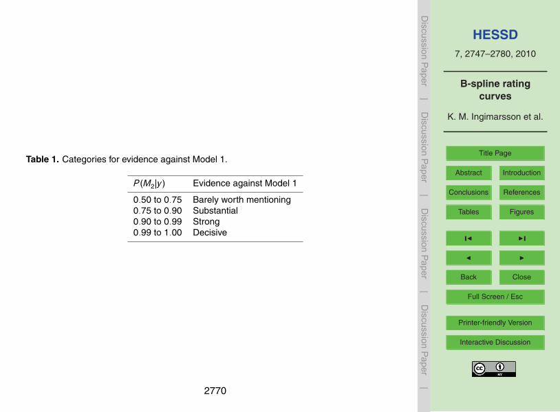
Kass and Raftery (1995) presented a table to categorize the evidence against a nullmodel (based on a table from Jeffreys, 1961). Here, the null model and the alternativemodel would be Model 1 and Model 2, respectively. If the Bayes factor values, whichmark the categories, are transformed to P (M2|y) (rounding the numbers from Kass andRaftery (1995) slightly) then the categories presented in Table 1 arise.15

Here the evidence against Model 1 is preferred to be strong or decisive (P (M2|y)>0.90) along with a DIC difference of ten or more, favoring Model 2, for the selection ofModel 2 over Model 1. The prior probabilities are selected as P (Mi )=0.5, i =1,2.

One way to compute B12 is by evaluating the integrals∫Θipi (y|θ i )pi (θ i )dθ i , i =1,2,

with the formula20 1T

T∑t=1

1

pi(y|θ (t)

i

)

−1

2753





HESSD7, 2747–2780, 2010



Title Page



Tables Figures

J I

J I

Back Close

Full Screen / Esc



Discussion

Paper

|D

iscussionP

aper|

Discussion

Paper

|D

iscussionP

aper|

where θ(t)i is the t-th posterior sample of θ i . See Robert (2007) for details.

4 Models

A Bayesian model for discharge rating curves based on the standard power-law is givenby

qi =a(wi −c)b+εi , i =1,...,n,5

where n is the number of observations for a given site, (wi ,qi ) denotes the i -th pair ofobservations and εi is a mean zero measurement error such that

εi ∼N(0,η2(wi −c)2bψ ),

where a, b and c are as in Eq. (1), the parameter ψ controls how the error variancebehaves as a function of the expected value of q, and η2 is a scaling parameter for the10

variance. In essence this is the same model as the one presented by Petersen-Øverleir(2004) and it is currently used at IMO. The parameter a is a function of ϕ and b, thatis,

a=exp(α0+α1b+ϕ) (2)

where α0 = 4.9468 and α1 =−0.7674. This reparametrization is motivated by correla-15

tion between estimates of ln(a) and b, denoted by ln(a) and b, which are based on datafrom IMO, and the values for α0 and α1 are selected such that the correlation betweenln(a) and ln(a)−α0−α1b is zero (Arnason, 2005).

A new model referred to as Model 2 is proposed. The form of this model is given by

qi =E(q(wi ))+εi , i =1,...,n,20

where εi is an error term such that

εi ∼N(

0,η2(wi −c2)2b2

), i =1,...,n, (3)

2754





HESSD7, 2747–2780, 2010



Title Page



Tables Figures

J I

J I

Back Close

Full Screen / Esc



Discussion

Paper

|D

iscussionP

aper|

Discussion

Paper

|D

iscussionP

aper|

and η2, b2 and c2 are unknown parameters. The observed discharge is always positiveso qi is normally distributed under the constraint qi > 0. The variance of Model 2 waschosen to be essentially the same as the variance in Model 1. Note that b2 and c2play a similar role as ψb and c in the variance of Model 1. However, the variance ofModel 2 does not include parameters of the mean function. This is done to simplify the5

conditional distributions of the Gibbs sampler and obtain more stable simulation fromthe posterior distribution. The expected value of q(w) is given by

E(q(w))=

a(w−c)b, w >wupp

a(w−c)b+∑Ll=1λlGl (w), wlow <w ≤wupp

a(w−c)b+λ1, w0 ≤w ≤wlow

(4)

where λL = 0, and the parameter space of a, b, c and λ is such that E(q(w))≥ 0. Notethat E(q(w)) is not defined for w <w0. The coefficient λL is set equal to zero to ensure10

continuity at wupp. The terms Gl (w) are such that

Gl (w)=Bl

(w−wlow

wupp−wlow

), wlow ≤w ≤wupp,

for l = 1,...,L. The terms Bl (z), l = 1,...,L, are cubic B-splines (Wasserman, 2006)which have support on the interval z ∈ [0,1], wlow and wupp are the lower and upperpoints, respectively, of the interval influenced by the B-splines. For a given river the15

quantities wmin and wmax are the smallest and the largest observed water level, re-spectively, within the pairs (wi ,qi ), i = 1,...,n. Based on time series for a particularriver, the smallest water level ever observed is found and is denoted by w0.

The quantity wupp should be selected close to wmax as the data points above wupphave little influence on the B-spline part but mainly influence the power-law curve and20

thus strengthen the estimation of the parameters of the power-law. For values abovewupp the fitted curve is only based on the power-law curve as Eq. (4) indicates. How-ever, wupp should be smaller than wmax as leaving no data points above wupp will take

2755





HESSD7, 2747–2780, 2010



Title Page



Tables Figures

J I

J I

Back Close

Full Screen / Esc



Discussion

Paper

|D

iscussionP

aper|

Discussion

Paper

|D

iscussionP

aper|

away information from the parameters of the power-law curve, in particular if the am-plitude of the B-spline part is large. This would also result in less accurate predictionof discharge above wupp. However, there is always some information on the power-lawparameters in the data points below wupp, especially in the data points that are closeto wupp. This is partly due to the fact that λL is set equal to zero. Selecting wupp much5

smaller than wmax results in less flexibility of the model since the B-spline part is theneffective over a smaller range of water level values. If that is done the power-law aloneis used to fit over a larger range of water level values which may result in a biased fit ifthere are substantial deviations from a single power-law curve above the selected wupp.Hence, when selecting wupp, there is a trade-off between a good fit below wmax and cer-10

tainty in prediction intervals for water level above wmax. Here, a good fit is preferred atthe cost of certainty in prediction. However, wupp is not set equal to wmax but a few datapoints are left to direct the power-law curve for values above wupp. In order to evaluatethe appropriate choice of wupp the ability of the model to predict discharge above wmaxwas evaluated for three choices of wupp. The quantity wupp was set equal to the sec-15

ond largest (w(n−1)), the third largest (w(n−2)) and the fourth largest (w(n−3)) water levelmeasurement but these three choices of wupp where deemed to be the ones leadingto good prediction properties and good fit. To evaluate these three choices of wupp alldata sets with fourteen or more pairs of observations were analyzed. In each case, thethree observations with the largest observed water level were omitted in estimation of20

the rating curve and predicted with the fitted rating curve. The sum of squared resid-uals was used to compare the three choices of wupp in Model 2. Table 2 shows thepercentage of times the three models give the best prediction, the second best predic-tion and the third best prediction. The choice with wupp equal to the third largest waterlevel measurement gave predictions that were the best and the second best in most25

cases. Since the differences between the best and the second best prediction wereusually small, wupp is set equal to the third largest water level observation.

The lower end of the effective range of the B-spline, wlow, is set equal to w0 to ensurethat the fitted curve is influenced by the B-spline for all water level values below wupp

2756





HESSD7, 2747–2780, 2010



Title Page



Tables Figures

J I

J I

Back Close

Full Screen / Esc



Discussion

Paper

|D

iscussionP

aper|

Discussion

Paper

|D

iscussionP

aper|

and down to the smallest water level for which discharge is predicted. If wlow would beset equal to a value greater than wmin the same power-law curve alone would applyto both large and small water level values and restrict the flexibility of the model. Thechoice wlow =w0 will minimize the effect of the data points with the smallest water levelobservations on the parameters of the power law. The coefficient corresponding to5

the first B-spline kernel, λ1, is allowed to be non-zero to introduce more flexibility tothe model. Hence at wlow the fitted curve deviates by amount equal to λ1 from thepower-law. The above selection of wlow and wupp leads then to the following ordering:

w0 =wlow ≤wmin <wupp <wmax.

The B-spline parameters in λ= (λ1,...,λL) are unknown (with the constraint that λL =10

0) where L is the number of B-spline kernels. For simplicity reasons the number ofB-splines kernels is fixed (the value of L) and the spacing between the interior knots isalso fixed. Equally spaced B-splines are used to obtain consistent smoothness over theentire B-spline interval as well as to reduce computational complexity. It is not optimalto have fixed number of B-spline kernels but a reasonable number can be deduced by15

using DIC as a measure. Based on evaluation of the four discharge data sets shown inTable 3 it was found that choosing L equal to nine captures the potential improvementsgained by Model 2 compared to Model 1. Table 3 shows that there is a small differencein the DIC for values of L between seven and fifteen in favor of adding kernels. In thecase of Norðurá with L equal to five the model needs extra kernels to be able to fit the20

data accurately and it needs more than seven kernels to become stable. However, itis of course possible to select a number different from nine for individual data sets byoptimizing DIC or applying some other criteria.

5 Bayesian inference

The Bayesian approach requires specification of prior distributions for each of the un-25

known parameters. The normal prior distributions selected for ϕ, b, c and ψ in Model2757





HESSD7, 2747–2780, 2010



Title Page



Tables Figures

J I

J I

Back Close

Full Screen / Esc



Discussion

Paper

|D

iscussionP

aper|

Discussion

Paper

|D

iscussionP

aper|

1 are the same (with one exception) as those in Arnason (2005) where point estimatesof a, b and c calculated from several data set at IMO were used to construct a priorfor these parameters. The exception is the standard deviation in the normal density forb. Arnason (2005) used σb = 0.75 but in this paper σb = 0.4 is used. It is consideredsafe to decrease the value of σb since the previous value was based on point estimates5

which included sampling error. This prior is reasonable in terms of sensible values ofb. The prior of a was then transformed to the prior of ϕ according to Eq. (2). The priordistributions for ϕ, b and c are specified in Appendix. Note that the prior density forb, denoted by p(b), is a truncated normal density between 0.5 and 5 so values below0.5 and above 5 are assumed invalid. The posterior density of c will be influenced by10

its prior density which is denoted by p(c) and also by w0. Since c is the water level atwhich discharge is zero, values of c above w0 are invalid. A vague but a proper prior ischosen for η2 since the mean function for q is fairly well determined by the priors for theparameters in the mean function and the deviation of the data from the mean curve isallowed to form the posterior distribution. An inverse-χ2 prior distribution for η2 results15

in an inverse-χ2 conditional posterior distribution which is convenient when using theGibbs sampler. The hyperparameters in the prior distribution of η2 are chosen to havea minimal effect on the posterior distribution. The prior for η2 could be improved bycollecting point estimates of η2 based on past data sets. This improvement is left forfuture research.20

Some of the prior distributions for the parameters in Model 2 are the same as theprior distributions of corresponding parameters in Model 1. First, b, c, ϕ and η2 inModel 2 have the same prior distributions as b, c, ϕ and η2 in Model 1. The parameterc2 in Model 2 has the same prior distributions as c in Model 1. The prior distributionof b2 is constructed such that it has a distribution that is similar to that of b times ψ in25

Model 1.A normal Markov random field prior (Rue and Held, 2005) with mean zero and covari-

ance matrix τ2D(I−φC)−1MD is assumed for the B-spline coefficients, λ, (see also inAppendix). This prior works as a penalty for λ. The parameters τ2 and φ are unknown.

2758





HESSD7, 2747–2780, 2010



Title Page



Tables Figures

J I

J I

Back Close

Full Screen / Esc



Discussion

Paper

|D

iscussionP

aper|

Discussion

Paper

|D

iscussionP

aper|

In Marx and Eilers (2005) methods for multidimensional splines using classical statis-tics are discussed. The authors introduce penalty terms in their objective function forthe estimation of the spline coefficients. The prior distribution proposed here for the B-spline coefficients gives term in the logged posterior distribution which has a form verysimilar to the one dimensional penalty term in the objective function in Marx and Eilers5

(2005). The parameter τ2 plays the same role as one over the smoothing parameterin Marx and Eilers (2005). The parameter φ needs to be one to obtain the same ma-trices as in Marx and Eilers (2005). But for the prior on the B-spline coefficients to beproper φ needs to be less than one, in fact φ∈ [0,1). In order to have the prior workingsimilarly to the penalty in Marx and Eilers (2005), the prior for φ is selected such that it10

favors values very close to one. To accomplish this a beta prior distribution with α=20and β = 0.5 is selected for φ. This distribution has 90% of its mass between 0.93 and1. With these prior distributions forφ and λ rapid changes in consecutive λ are avoided,the uncertainty in the λs is reduced and the B-spline function is smoother than if φ wasequal to zero. It was also found that if φ= 0 then the Bayesian computation becomes15

unstable and the λs do not converge to an optimal value.The parameter τ2 controls the size of the elements of λ. A vague inverse-χ2 prior is

chosen for τ2 due to the lack of knowledge about sensible values for this parameter.This prior allows the posterior distribution to put a lot of mass close to zero which is adesirable property since in many cases τ2 is in fact equal to zero (the B-spline part is20

zero). The prior for τ2 also puts a lot of mass on larger values of τ2. The variability inthe data is bounded which in turn bounds the variability in the posterior distribution ofτ2.

The matrices D and M are diagonal with known constants on their diagonals and Cis a constant first order neighborhood matrix. The role of D is to let the prior variance25

of the λ’s decrease as the index goes from 1 to L which forces the B-spline part tobecome smaller as w approaches wupp therefore it could be used to further force themodel to be smooth at the wupp. However, in this paper D is set equal to the identity

2759





HESSD7, 2747–2780, 2010



Title Page



Tables Figures

J I

J I

Back Close

Full Screen / Esc



Discussion

Paper

|D

iscussionP

aper|

Discussion

Paper

|D

iscussionP

aper|

matrix. The role of the matrix M is to adjust for the end points. M is such that

Ml l =0.5, ,l =2,...,L−1, M11 =MLL =1.

The neighborhood matrix C is such that

Cl ,l−1 =Cl ,l+1 =0.5, ,l =2,...,L−1,

and C12 =CL,L−1 = 1. The posterior distribution of θ = (ϕ,b,c,η2,b2,c2,λ,τ2,φ) given5

the data q= (q1,...,qn), w = (w 1,...,w n), is given by

p(θ ||q,w )∝n∏i=1

p(qi |θ ,wi )×p(ϕ)p(b)p(c)p(η2)×p(b2)p(c2)p(λ|τ2,φ)p(τ2)p(φ)

(5)

where p(qi |θ ,wi ) is a normal density with mean as in Eq. (4) and variance as in Eq. (3).The part

∏ni=1p(qi |θ ,wi ) is the likelihood function which is used for the computation of10

DIC and Bayes factor.The inference about the unknown parameters is based on samples from the poste-

rior distribution which are generated by a Markov chain Monte Carlo (MCMC) simula-tion. A Gibbs sampler with Metropolis-Hastings steps is used for the MCMC simulationwhich consists of the conditional distributions of the unknown parameters (see Gelman15

et al. (2004) for further details on MCMC and the Gibbs sampler). The conditionaldistributions of η2 and τ2 are scaled inverse chi-square distributions. The conditionaldistributions of λ is a multivariate normal distribution where λ is first generated with-out any constraints then the constraint λL = 0 is taken into account. To generate fromthe conditional distributions of ϕ, b, c, b2, c2 and φ, a Metropolis–Hastings steps is20

needed in each case. However in Model 2 the values for the parameters c and c2are set equal to constant values, namely, their posterior medians, which were found byusing the Gibbs sampler. Other parameters in the model are estimated again with cand c2 fixed, resulting in more reliable estimates.

2760





HESSD7, 2747–2780, 2010



Title Page



Tables Figures

J I

J I

Back Close

Full Screen / Esc



Discussion

Paper

|D

iscussionP

aper|

Discussion

Paper

|D

iscussionP

aper|

For the unknown parameters of Model 1 and Model 2 four separate chains of itera-tions are used. Each chain takes a number of iterations to converge. Those iterationsare thrown away and referred to as burn-in period. The decision on the length of theburn-in period is based on the data set that took the longest time to converge. Bothmodels rely the same total number of iterations or 450 thousand. Model 1 than has a5

burn-in period of 390 thousand iterations. Every fourth value of each chain was storedafter the burn-in period to reduce correlation between iterations, yielding four chainsof length 15 thousand for posterior inference. For Model 2 the first burn-in period cov-ers the first quarter of each chain. The parameters c and c2 are estimated from theiterations in the second quarter of each chain. A second burn-in period starts after10

the first half of each chain. Out of the 60 thousand remaining iterations every fourthvalue of each chain is stored as in Model 1. Posterior simulations for both Model 1 andModel 2 were stable and the simulated chains converged in all cases. However, it isworth mentioning that in many cases both models converge when the total number ofiterations is 160 thousand.15

6 Results

In this section the two models introduced in Sect. 4 are applied to the 61 data sets fromIMO database for comparison between the two models. As mentioned in Sect. 2 fourof the data sets are analyzed in detail. These four data sets are from Norðurá, Jökulsáá Fjöllum, Jökulsá á Dal and Skjálfandafljót. Figure A shows the fitted discharge rating20

curves of the two models for these four data sets, along with prediction intervals andposterior intervals for the discharge rating curves.

In all cases, except for Jökulsá á Fjöllum, the 95% prediction intervals are wider forlarger values of water level in Model 1 than in Model 2. This is mainly due to the factthat if the fit through the observations is adequate then the variability around the fitted25

curve is smaller when compared to the variability around a poorer fit, this in turn resultsin narrower prediction intervals.

2761





HESSD7, 2747–2780, 2010



Title Page



Tables Figures

J I

J I

Back Close

Full Screen / Esc



Discussion

Paper

|D

iscussionP

aper|

Discussion

Paper

|D

iscussionP

aper|

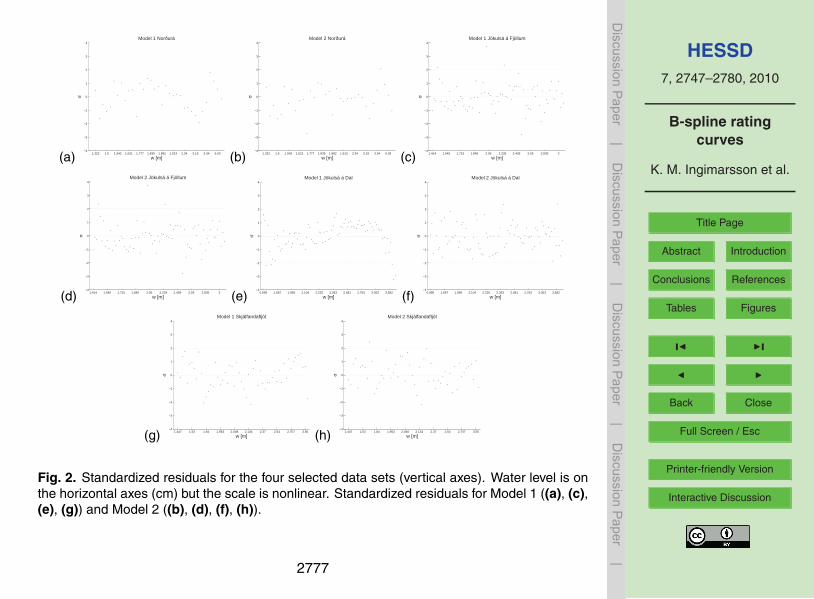
Figure 2 shows the standardized residuals of the two models versus water level.In general, when an adequate model is used then the standardized residuals shouldnot show any trend and appear to have the same variance for all values of the waterlevel. In the case of Norðurá, Model 2 yields more convincing standardized residualsthan Model 1, which shows a trend in the standardized residuals while that is not the5

case for Model 2. In the case of Jökulsá á Fjöllum there is no visible difference in thestandardized residuals which indicates that Model 2 imitates Model 1 when Model 2does not provide significant improvement over Model 1. For Jökulsá á Dal the trendin the standardized residuals of Model 1 is obvious, while the standardized residualsof Model 2 show no trend. In the case of Skjálfandafljót, there appears to be a trend10

in the standardized residuals of Model 1 for water level values lower than 1.84 m andgreater than 2.37 m while the standardized residuals of Model 2 show no trend. Thesefour examples demonstrate that Model 2 can provide better results than Model 1 andwhen Model 1 appears to be adequate, Model 2 performs as well as Model 1.

Figure 3 shows the roles that the standard power-law part and the B-spline part15

play in Model 2 for the four rivers. The B-spline part models the variation in the datafor the values of the water level below wupp that the standard power-law part can notadjust for on its own. The B-spline part is zero at and above wupp and it smoothlyapproaches zero as w approaches wupp from below. In the case of Norðurá as well asSkjálfandafljót the B-spline part allows Model 2 to give a visibly better fit. The standard20

power-law model (Model 1) is adequate in the case of Jökulsá á Fjöllum as is seen inthe left panel of Fig. 3. The right panel shows clearly the ability of the B-spline part ofModel 2 to reduce to almost zero, thus, the B-spline addition has insignificant effect onthe discharge rating curve for such case. In case of Jökulsá á Dal it can be seen thatthe B-spline part can take as large values as needed when the standard power-law25

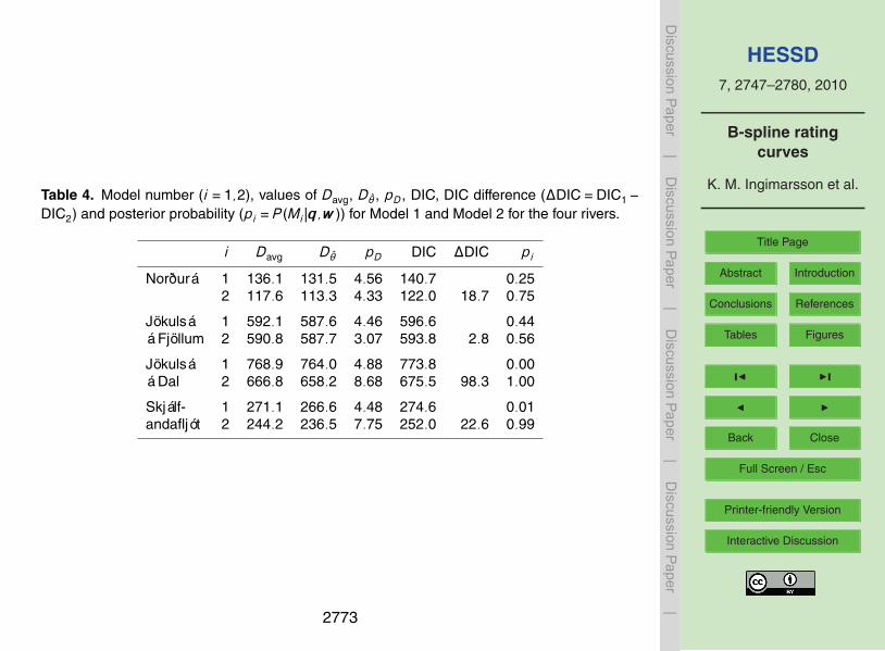
part is inadequate for the data set.In Table 4, a comparison between the two models is made through DIC and Bayes

factor (see Sect. 3). Table 4 shows that pD is less than the actual number of unknownparameters in Model 1 and Model 2 which are 5 and 15, respectively. This is expected

2762





HESSD7, 2747–2780, 2010



Title Page



Tables Figures

J I

J I

Back Close

Full Screen / Esc



Discussion

Paper

|D

iscussionP

aper|

Discussion

Paper

|D

iscussionP

aper|

due to the fact that the prior distributions constrain the unknown parameters. It seemsthat the more the B-spline part is contributing, the larger the number of effective pa-rameters. This shows the adaptive nature of the Markov random field prior for λ.

Table 4 shows that in all cases except Jökulsá á Fjöllum, Model 2 has considerablylower DIC than Model 1 indicating better fit for Model 2. The difference in DIC between5

Model 1 and Model 2 is about 19 and 23 for Norðurá and Skjálfandafljót, respectively,and about 98 for Jökulsá á Dal. In the case of DIC these are all relatively large differ-ences. In the case of Jökulsá á Fjöllum the difference in DIC is less than 3 which isviewed as a small difference. This is reflected in the fitted discharge rating curves ofModel 1 and Model 2 which show no visible differences for Jökulsá á Fjöllum in Fig. 3.10

The results in Table 4 and Figs. 2, 3 and 4 show that the B-spline part of Model 2 eitherimproves the fit compared to Model 1 or gives a fit equally good as that of Model 1 whenModel 1 is adequate. The posterior probability of Model 2 (based on Bayes factor) isalso computed for the four selected data sets in Table 4. The computed probability val-ues confirm that the DIC differences for Norðurá, Jökulsá á Dal and Skjálfandafljót are15

relatively large and support selecting Model 2 over Model 1. The posterior probabilityof Model 2 is close to 0.5 for Jökulsá á Fjöllum implying that Model 1 and Model 2 givesimilar results.

Figure 4 shows comparison between Model 1 and Model 2 for 61 stations analyzedfrom the IMO database by plotting the difference in DIC between the Model 2 and20

Model 1 on the horizontal axis (positive if Model 2 gives a better fit) and the posteriorprobability of Model 2 on the vertical axis. When the DIC difference is greater than tenand the posterior probability of Model 2 is greater than 0.9, then Model 2 significantlyimproves the fit of Model 1 (see Sect. 3). This is the case for 16 rivers which is about26% of the data sets. When the probability of Model 2 is between 0.0 and 0.90 and the25

DIC diffence is less than 10 then Model 2 is not outperforming Model 1 and that Model1 is adequate. This is the case for 36 rivers out of 61, or 59%. In case when the DICdifference is less than 10 and the posterior probability of Model 2 is greater than 0.9(7 of 61), and in the case when the DIC difference is greater than 10 and the posterior

2763





HESSD7, 2747–2780, 2010



Title Page



Tables Figures

J I

J I

Back Close

Full Screen / Esc



Discussion

Paper

|D

iscussionP

aper|

Discussion

Paper

|D

iscussionP

aper|

probability of Model 2 is less than 0.9 (2 of 61), a close look at the descriptive plots andstatistics is needed to determine whether Model 1 is adequate or not. This is true ingeneral, that is, a detailed analyzes of each data set is needed before a final decisionabout Model 1 or Model 2 is made. The DIC difference and the posterior probabilityof Model 2 are important measures to support that decision. It is however noted that5

Model 2 never yields worse results than Model 1. Model 2 only fails to improve Model1 in some cases, so Model 2 could be used in all cases.

Table 5 shows estimates of the parameters a, b and c which are sufficient to con-struct discharge rating curves based on standard power-law. These parameters arepresented for both Model 1 and Model 2. There is a substantial difference in these10

parameters between Model 1 and Model 2 which is due to the extra flexibility of Model2. The B-spline part in Model 2 has the ability to utilize information from lower valuesof water level in the data and therefore the standard power-law parameters can be es-timated with a more focus on the higher water level when needed. This can lead to adifferent posterior density for a, b and c in the two models as seen in Table 5.15

In Table 6, a posterior interval is given for rest of the parameters in Model 1 and inModel 2 except for λ. For Model 1 the parameter ψ is multiplied by b so it can becompared to the parameter b2 in Model 2. The posterior median of τ2 varies from2.99 in Jökulsá á Fjöllum to 1180.6 in Jökulsá á Dal which shows the difference in theamplitude of the B-spline part for these data sets. The parameter φ is forced to be20

close to one through its prior distribution to ensure strong positive correlation betweenthe elements of λ. The effect of the prior is clear in the posterior estimates of φ.

As discussed in Sect. 1, discharge rating curves are frequently used in extrapolationof discharge. As a demonstration, the three highest water level observations, alongwith corresponding discharges observations, were excluded from the data sets for the25

four rivers previously analysed. Then both models were used to extrapolate over therange of the three excluded water level values. Figure 5 shows the results. In all casesthe three excluded discharge values are within the 95% prediction interval for Model 2but only in two cases for Model 1, namely, Jökulsá á Fjöllum and Norðurá. For these

2764





HESSD7, 2747–2780, 2010



Title Page



Tables Figures

J I

J I

Back Close

Full Screen / Esc



Discussion

Paper

|D

iscussionP

aper|

Discussion

Paper

|D

iscussionP

aper|

two cases the models are similar for Jökulsá á Fjöllum but Model 2 looks better forNorðurá. For the other two cases Model 1 is considerably of the mark. From these fourcases it can be concluded that Model 2 performs considerably better or equally goodin predicting discharge for extrapolated water level values greater than wmax.

Model 1 and Model 2 (with wupp equal to the third largest water level observation) are5

compared in terms of prediction. For that comparison only 48 data sets could be usedsince, as described above, the three highest water level were excluded in estimationof parameters. Model 2 performed better than Model 1 for 29 data sets out of 48 or incase of 60% of data sets. However, in terms of fitting the data, 16 data sets out of 61are such that Model 2 is judged to give a better fit than Model 1. So, in some cases10

even if the fit for Model 1 is better than or equally good as that of Model 2, then Model 2appears to perform better when predicting discharge for water level greater than wmax.However, in few cases Model 1 performs better when predicting discharge for waterlevel greater than wmax even though Model 2 gives a better fit.

7 Conclusions15

A Bayesian model for discharge rating curves, labeled Model 2, was developed by ex-tending the standard power-law model, labeled Model 1, by adding a B-spline function.Comparison of these two models based on analysis of 61 data sets from IMO showsthat Model 2 outperforms or performs as well as Model 1. One of the most importantproperties of Model 2 is the capacity of the B-spline part to catch deviation in the data20

from the standard power-law model when that model is inadequate. In these cases,Model 2 achives a more convincing fit to the data than Model 1. This is confirmed withcalculations of DIC and Bayes factor where Model 2 yields a substantially lower DICvalues and higher posterior probabilities than Model 1 in 16 of 61 cases (DIC differencegreater than ten and posterior probability of Model 2 greater than 0.9). In 36 cases the25

DIC difference is less than ten and the posterior probability of Model 2 less than 0.9and it is debatable whether the added complexity of Model 2 leads to an improvement.

2765





HESSD7, 2747–2780, 2010



Title Page



Tables Figures

J I

J I

Back Close

Full Screen / Esc



Discussion

Paper

|D

iscussionP

aper|

Discussion

Paper

|D

iscussionP

aper|

Another important property of Model 2 is that when Model 1 gives an adequate fit, asin the case of Jökulsá á Fjöllum, Model 2 imitates Model 1 by reducing the amplitude ofthe B-spline almost down to zero. Model 2 performs better than Model 1 when it comesto prediction of discharge for water level above wmax as it gives better results for 60%of the analyzed data sets, which supports the use of Model 2.5

It is concluded that Model 2 can be used to fit discharge rating curves regardless ofwhether the standard power-law model is adequate or not. The exception is when thedata sets contain few data pairs so there may not be enough information to estimatethe B-spline part successfully. Based on the experience gained in the present analysisat least ten data pairs are needed.10

Finally, it is noted that segmentation has been commonly used in estimating dis-charge rating curves and it could be argued that maybe it is more appropriate thanModel 2 for data sets where there is visually an apparent shift. A direct comparisonbetween segmentation models and Model 2 is needed to compare their performance.A joint use of multi-segment discharge rating curves and B-splines could potentially be15

beneficial for such cases.

2766





HESSD7, 2747–2780, 2010



Title Page



Tables Figures

J I

J I

Back Close

Full Screen / Esc



Discussion

Paper

|D

iscussionP

aper|

Discussion

Paper

|D

iscussionP

aper|

Appendix A

Prior distributions

The following prior distributions are proposed for the unknown parameters.p(ϕ)=N(ϕ|µϕ =0,σ2

ϕ =0.822)p(b)∝N(b|µb =2.15,σ2

b =0.42)I(0.5<b< 5)p(c)∝N(c|µc =75,σ2

c =502)I(c<w0)p(ψ)∝N(ψ |µψ =0.8,σ2

ψ =0.252)I(0<ψ < 1.2)p(b2)∝N(b2|µb2 =2.15,σ2

b2 =0.42)I(1<b< 6)p(c2)∝N(c2|µc2 =75,σ2

c2 =502)I(c2 <w0)p(η2)∝ Inv−χ2(η2|νη =10−12,S2

η =1)p(φ)=Beta(φ|αφ =20,βφ =0.5)p(τ2)∝ Inv−χ2(τ2|ντ =10−12,S2

τ =1)p(λ|τ2,φ)∝N(λ|0,τ2D(I−φC)−1MD)

5

where I(A) is such that I(A) = 1 if A is true and I(A) = 0 otherwise. In the priordistribution for λ, I is an identity matrix, D and M are diagonal matrices and C is aneighborhood matrix with constants on the first off-diagonals, other elements are equalto zero.10

2767





HESSD7, 2747–2780, 2010



Title Page



Tables Figures

J I

J I

Back Close

Full Screen / Esc



Discussion

Paper

|D

iscussionP

aper|

Discussion

Paper

|D

iscussionP

aper|

References

Arnason, S.: Estimating nonlinear hydrological rating curves and discharge using the Bayesianapproach., Masters thesis, Faculty of Engineering, University of Iceland, 2005. 2749, 2750,2754, 2758

Clarke, R.: Uncertainty in the estimation of mean annual flood due to rating-curve indefinition,5

J. Hydrol., 222, 185–190, 1999. 2749Di Baldassarre, G. and Montanari, A.: Uncertainty in river discharge observations: a quantita-

tive analysis, Hydrol. Earth Syst. Sci., 13, 913–921, 2009,http://www.hydrol-earth-syst-sci.net/13/913/2009/. 2749

Gelman, A., Carlin, J., Stern, H., and Rubin, D.: Bayesian Data Analysis, Chapman and10

Hall/CRC, 2nd edn., Boca Raton, Florida, USA, 2004. 2752, 2760ISO: Liquid flow measurements in open channels, Handbook 16, International Standards Or-

ganization, 1983. 2748Jeffreys, H.: Theory of probability, University Press, Oxford, UK, 3rd edn., 1961. 2753Kass, R. and Raftery, A.: Bayes factors and model uncertainty, J. Am. Stat. Assoc., 90, 773–15

795, 1995. 2753Lambie, J.: Measurement of flow-velocity-area methods, in: Hydrometry: Principles and Prac-

tices, edited by: Herschy, R. W., John Wiley & Sons Ltd, Chichester, UK, 1–52, 1978. 2749Lohani, A., Goel, N., and Bhatia, K.: Takagi–Sugeno fuzzy inference system for modeling

stage–discharge relationship, J. Hydrol., 331, 146–160, 2006. 2750, 275120

Marx, B. and Eilers, P.: Multidimensional penalized signal regression, Technometrics, 47, 13–22, 2005. 2759

Mosley, M. and McKerchar, A.: Streamflow, in: Handbook of Hydrology, edited by: Maidment,D. R., McGraw Hill, New York, USA, 8.1–8.39, 1993. 2748, 2749

Moyeed, R. and Clarke, R.: The use of Bayesian methods for fitting rating curves, with case25

studies, Adv. Water Resour., 28, 807–818, 2005. 2749Pelletier, P.: Uncertainties in the single determination of river discharge: a literature review,

Can. J. Civil Eng., 15, 834–850, 1988. 2749Petersen-Øverleir, A.: Accounting for heteroscedasticity in rating curve estimates, J. Hydrol.,

292, 173–181, 2004. 2750, 275430

Petersen-Øverleir, A. and Reitan, T.: Objective segmentation in compound rating curves, J.Hydrol., 311, 188–201, 2005. 2750

2768





http://www.hydrol-earth-syst-sci.net/13/913/2009/

HESSD7, 2747–2780, 2010



Title Page



Tables Figures

J I

J I

Back Close

Full Screen / Esc



Discussion

Paper

|D

iscussionP

aper|

Discussion

Paper

|D

iscussionP

aper|

Reitan, T. and Petersen-Øverleir, A.: Bayesian methods for estimating multi-segment dischargerating curves, Stoch. Env. Res. Risk A., 23, 1–16, 2008a. 2750

Reitan, T. and Petersen-Øverleir, A.: Bayesian power-law regression with a location parameter,with applications for construction of discharge rating curves, Stoch. Env. Res. Risk A., 22,351–365, 2008b. 27495

Robert, C.: The Bayesian choice: from decision-theoretic foundations to computational imple-mentation, Springer Verlag, New York, USA, 2007. 2754

Rue, H. and Held, L.: Gaussian Markov Random Fields: Theory and Applications, Chapman &Hall/CRC, Boca Raton, Florida, USA, 2005. 2758

Spiegelhalter, D., Best, N., Carlin, B., and van der Linde, A.: Bayesian measures of model10

complexity and fit, J. Roy. Stat. Soc. B, 64, 583–639, 2002. 2752Wasserman, L.: All of Nonparametric Statistics, Springer Verlag, New York, USA, 2006. 2755

2769





HESSD7, 2747–2780, 2010



Title Page



Tables Figures

J I

J I

Back Close

Full Screen / Esc



Discussion

Paper

|D

iscussionP

aper|

Discussion

Paper

|D

iscussionP

aper|

Table 1. Categories for evidence against Model 1.

P (M2|y) Evidence against Model 1

0.50 to 0.75 Barely worth mentioning0.75 to 0.90 Substantial0.90 to 0.99 Strong0.99 to 1.00 Decisive

2770





HESSD7, 2747–2780, 2010



Title Page



Tables Figures

J I

J I

Back Close

Full Screen / Esc



Discussion

Paper

|D

iscussionP

aper|

Discussion

Paper

|D

iscussionP

aper|

Table 2. The prediction performance of Model 2 when wupp was set equal to the second largest(w(n−1)), the third largest (w(n−2)) and the fourth largest (w(n−3)) water level measurement. Thetable shows the percentage of times selected value of wupp yields the best prediction, thesecond best prediction and the third best prediction. The total number of datasets used was48.

wupp w(n−1) w(n−2) w(n−3)

Best prediction 39.6% 29.2% 31.2%2nd best prediction 22.9% 47.9% 29.2%3rd best prediction 37.5% 22.9% 39.6%

2771





HESSD7, 2747–2780, 2010



Title Page



Tables Figures

J I

J I

Back Close

Full Screen / Esc



Discussion

Paper

|D

iscussionP

aper|

Discussion

Paper

|D

iscussionP

aper|

Table 3. The values of pd , DIC, for different number of L in Model 2 for the four rivers.

J. Fjöllum NorðuráL pd DIC pd DIC

5 3.27 594.35 3.00 134.307 3.12 594.23 0.95 118.129 3.07 593.84 4.33 121.9511 3.08 593.65 4.99 123.1913 3.14 593.27 5.94 124.6515 3.07 592.97 5.95 125.17

J. Dal Skjálf.

5 6.32 676.96 5.63 255.047 7.80 673.95 6.95 253.799 8.68 675.50 7.75 251.9811 10.00 675.92 8.29 252.9813 10.91 675.48 8.95 251.6715 11.53 674.57 9.50 251.57

2772





HESSD7, 2747–2780, 2010



Title Page



Tables Figures

J I

J I

Back Close

Full Screen / Esc



Discussion

Paper

|D

iscussionP

aper|

Discussion

Paper

|D

iscussionP

aper|

Table 4. Model number (i = 1,2), values of Davg, Dθ, pD, DIC, DIC difference (∆DIC=DIC1 −DIC2) and posterior probability (pi = P (Mi |q,w )) for Model 1 and Model 2 for the four rivers.

i Davg Dθ pD DIC ∆DIC pi

Norðurá 1 136.1 131.5 4.56 140.7 0.252 117.6 113.3 4.33 122.0 18.7 0.75

Jökulsá 1 592.1 587.6 4.46 596.6 0.44á Fjöllum 2 590.8 587.7 3.07 593.8 2.8 0.56

Jökulsá 1 768.9 764.0 4.88 773.8 0.00á Dal 2 666.8 658.2 8.68 675.5 98.3 1.00

Skjálf- 1 271.1 266.6 4.48 274.6 0.01andafljót 2 244.2 236.5 7.75 252.0 22.6 0.99

2773





HESSD7, 2747–2780, 2010



Title Page



Tables Figures

J I

J I

Back Close

Full Screen / Esc



Discussion

Paper

|D

iscussionP

aper|

Discussion

Paper

|D

iscussionP

aper|

Table 5. Posterior estimates of a, b and c in Model 1 and Model 2.

Mod. 1 Mod. 2a b c a b c

N.áPost. med. 15.7 2.16 0.88 9.6 2.45 0.69∗

2.5 perc. 11.7 2.06 0.77 6.5 1.9497.5 perc. 17.5 2.36 0.93 21.1 2.75

J. á Fj.Post. med. 69.9 2.13 0.29 66.0 2.16 0.25∗

2.5 perc. 49.4 1.94 0.11 59.4 2.0397.5 perc. 92.2 2.34 0.43 75.4 2.27

J. á DalPost. med. 112.7 1.68 0.74 107.9 1.48 0.44∗

2.5 perc. 92.6 1.52 0.64 73.6 1.2297.5 perc. 135.0 1.87 0.82 151.1 1.76

Skj.fl.Post. med. 7.6 3.01 0.06 24.4 2.39 0.58∗

2.5 perc. 4.1 2.85 −0.18 20.7 2.2397.5 perc. 10.1 3.36 0.18 29.0 2.54

* c is pre-estimated and therefore a constant, as explained in Sect. 5.

2774





HESSD7, 2747–2780, 2010



Title Page



Tables Figures

J I

J I

Back Close

Full Screen / Esc



Discussion

Paper

|D

iscussionP

aper|

Discussion

Paper

|D

iscussionP

aper|

Table 6. Posterior estimates of ψ×b and η2 in Model 1 and b2, c2, η2, τ2 and φ in Model 2.

Mod. 1 Mod. 2ψ×b η2 b2 c2 η2 τ2 φ

NorðuráPost. median 2.42 0.05 2.71 0.62∗ 0.22 19.80 0.952.5 percentile 2.12 0.02 2.30 0.12 0.32 0.8097.5 percentile 2.63 0.15 3.12 0.47 597.33 0.99

Jökulsá á Fj.Post. median 1.77 1.04 2.02 0.15∗ 8.87 2.99 0.952.5 percentile 1.17 0.06 1.48 4.14 0.0004 0.8197.5 percentile 2.57 21.64 2.55 20.32 136.74 0.99

Jökulsá á DalPost. median 1.44 4.74 1.96 −0.19∗ 3.77 1180.6 0.962.5 percentile 1.03 0.84 1.52 1.67 437.8 0.8397.5 percentile 1.84 45.17 2.40 9.09 4274.6 0.99

Skjálfandaflj.Post. median 2.75 0.024 2.03 0.11∗ 0.26 17.11 0.952.5 percentile 1.98 0.002 1.43 0.11 3.88 0.8297.5 percentile 3.72 0.231 2.63 0.64 79.43 0.99

* c2 is pre-estimated and therefore a constant as explained in Sect. 5.

2775





HESSD7, 2747–2780, 2010



Title Page



Tables Figures

J I

J I

Back Close

Full Screen / Esc



Discussion

Paper

|D

iscussionP

aper|

Discussion

Paper

|D

iscussionP

aper|

(a)0 100 200 300 400 500 600 700

1

1.5

2

2.5

3

3.5

4

4.5

5

5.5

6

q [m3/sec]

w [m

]

Model 1 Norðurá

(b)0 100 200 300 400 500 600 700

1

1.5

2

2.5

3

3.5

4

4.5

5

5.5

6

q [m3/sec]

w [m

]

Model 2 Norðurá

(c)0 200 400 600 800 1000 1200

0.5

1

1.5

2

2.5

3

3.5

4

q [m3/sec]

w [m

]

Model 1 Jökulsá á Fjöllum

(d)0 200 400 600 800 1000 1200

0.5

1

1.5

2

2.5

3

3.5

4

q [m3/sec]

w [m

]


(e)0 200 400 600 800 1000 1200 1400 1600 1800

0.5

1

1.5

2

2.5

3

3.5

4

4.5

5

5.5

q [m3/sec]

w [m

]

Model 1 Jökulsá á Dal

(f)0 200 400 600 800 1000 1200 1400

0.5

1

1.5

2

2.5

3

3.5

4

4.5

5

5.5

q [m3/sec]

w [m

]


(g)0 100 200 300 400 500 600 700 800

1

1.5

2

2.5

3

3.5

4

4.5

5

q [m3/sec]

w [m

]

Model 1 Skjálfandafljót

(h)0 100 200 300 400 500 600 700

1

1.5

2

2.5

3

3.5

4

4.5

5

q [m3/sec]

w [m

]Model 2 Skjálfandafljót

Fig. 1. The fit of Model 1 ((a), (c), (e), (g)) and of Model 2 ((b), (d), (f), (h)) to the four selecteddata sets. The vertical axes shows water level (w) in meters while the horizontal axes showsthe discharge (q), in m3/s. The black solid curves show the posterior median of E(q) and the95% posterior interval of E(q). The dotted curves show prediction intervals.

2776





HESSD7, 2747–2780, 2010



Title Page



Tables Figures

J I

J I

Back Close

Full Screen / Esc



Discussion

Paper

|D

iscussionP

aper|

Discussion

Paper

|D

iscussionP

aper|

(a) 1.322 1.5 1.542 1.621 1.777 1.835 1.882 1.913 2.34 3.19 3.34 5.03−4

−3

−2

−1

0

1

2

3

4Model 1 Norðurá

w [m]

σ

(b) 1.322 1.5 1.542 1.621 1.777 1.835 1.882 1.913 2.34 3.19 3.34 5.03−4

−3

−2

−1

0

1

2

3

4

w [m]

σ

Model 2 Norðurá

(c) 1.414 1.545 1.715 1.845 2.05 2.239 2.439 2.55 2.835 3−4

−3

−2

−1

0

1

2

3

4Model 1 Jökulsá á Fjöllum

w [m]

σ

(d) 1.414 1.545 1.715 1.845 2.05 2.239 2.439 2.55 2.835 3−4

−3

−2

−1

0

1

2

3

4

w [m]

σ


(e) 0.995 1.687 1.959 2.104 2.225 2.363 2.481 2.763 3.053 3.582−4

−3

−2

−1

0

1

2

3

4Model 1 Jökulsá á Dal

w [m]

σ

(f) 0.995 1.687 1.959 2.104 2.225 2.363 2.481 2.763 3.053 3.582−4

−3

−2

−1

0

1

2

3

4

w [m]

σ


(g) 1.447 1.53 1.84 1.953 2.048 2.134 2.37 2.54 2.707 3.56−4

−3

−2

−1

0

1

2

3

4Model 1 Skjálfandafljót

w [m]

σ

(h) 1.447 1.53 1.84 1.953 2.048 2.134 2.37 2.54 2.707 3.56−4

−3

−2

−1

0

1

2

3

4

w [m]

σ


Fig. 2. Standardized residuals for the four selected data sets (vertical axes). Water level is onthe horizontal axes (cm) but the scale is nonlinear. Standardized residuals for Model 1 ((a), (c),(e), (g)) and Model 2 ((b), (d), (f), (h)).

2777





HESSD7, 2747–2780, 2010



Title Page



Tables Figures

J I

J I

Back Close

Full Screen / Esc



Discussion

Paper

|D

iscussionP

aper|

Discussion

Paper

|D

iscussionP

aper|

(a)0 50 100 150 200 250 300 350 400

1

1.5

2

2.5

3

3.5

4

4.5

5

5.5

q [m3/sec]

w [m

]

Model 2 Norðurá

(b)−2.5 −2 −1.5 −1 −0.5 0 0.5 1 1.51

1.5

2

2.5

3

3.5

4

4.5

5

5.5

q [m3/sec]

w [m

]

Model 2 Norðurá

(c)0 100 200 300 400 500 600 700

0.5

1

1.5

2

2.5

3

3.5

q [m3/sec]

w [m

]


(d)−0.14 −0.12 −0.1 −0.08 −0.06 −0.04 −0.02 0 0.02 0.040.5

1

1.5

2

2.5

3

3.5

q [m3/sec]

w [m

]


(e)0 100 200 300 400 500 600 700 800

0.5

1

1.5

2

2.5

3

3.5

4

q [m3/sec]

w [m

]


(f)−60 −40 −20 0 20 40 60

0.5

1

1.5

2

2.5

3

3.5

4

q [m3/sec]

w [m

]


(g)0 50 100 150 200 250

1.4

1.6

1.8

2

2.2

2.4

2.6

2.8

3

3.2

q [m3/sec]

w [m

]


(h)−6 −4 −2 0 2 4 6

1.4

1.6

1.8

2

2.2

2.4

2.6

2.8

3

3.2

q [m3/sec]

w [m

]


Fig. 3. Figures (a), (c), (e) and (g) show shows the standard power-law part (solid red curves)of Model 2 and the sum of standard power-law part and the B-spline part of Model 2 (solidblack curves) for the four selected data sets. Figures (b), (d), (f) and (h) show the B-spline partof Model 2 for each data set. Water level is on the vertical axes (m) while discharge is on thehorizontal axes (m3/s).

2778





HESSD7, 2747–2780, 2010



Title Page



Tables Figures

J I

J I

Back Close

Full Screen / Esc



Discussion

Paper

|D

iscussionP

aper|

Discussion

Paper

|D

iscussionP

aper|

0 10 25 50 75 1000

0.1

0.25

0.5

0.75

0.9

1

DIC difference

Pro

babi

lity

of M

odel

2

Fig. 4. The difference in DIC between the two models is on the horizontal axis and the posteriorprobability of Model 2 (based on Bayes factor) is on the vertical axes.

2779





HESSD7, 2747–2780, 2010



Title Page



Tables Figures

J I

J I

Back Close

Full Screen / Esc



Discussion

Paper

|D

iscussionP

aper|

Discussion

Paper

|D

iscussionP

aper|

(a)0 200 400 600 800 1000 1200

1

2

3

4

q [m3/sec]

w [m

]

Prediction Jökulsá á Fjöllum

(b)0 100 200 300 400 500 600 700 800

1

2

3

4

5

6

q [m3/sec]

w [m

]

Prediction Norðurá

(c)0 200 400 600 800 1000 1200 1400 1600 1800

1

2

3

4

5

q [m3/sec]

w [m

]

Prediction Jökulsá á Dal

(d)0 100 200 300 400 500 600 700 800 900

1

2

3

4

5

q [m3/sec]

w [m

]

Prediction Sjálfandafljót

Fig. 5. The solid curves show the posterior median of E(q), red for Model 1 and black forModel 2 for the four selected data sets. The dotted curves show prediction intervals, red forModel 1 and black for Model 2. Water level is on the vertical axes (m) while discharge is on thehorizontal axes (m3/s).

2780





b-spline rating curves - hessd - recent · b-spline rating curves ... on b-spline smoothing...

Documents