Basic Concepts of Thermodynamics

Reading Problems2-1→ 2-8 2-44, 2-48, 2-78, 2-100

Thermal SciencesThe thermal sciences involve the storage, transfer and conversion of energy.

We will study the basic laws and principles that govern the three disciplines of thermal sciences,namely, thermodynamics, heat transfer and fluid mechanics.

Th

erm

od

yn

am

ics

Heat T

ran

sfer

Fluids Mechanics

Thermal

Systems

Engineering

Thermodynamics

Fluid Mechanics

Heat TransferConservation of mass

Conservation of energy

Second law of thermodynamics

Properties

Fluid statics

Conservation of momentum

Mechanical energy equation

Modeling

Conduction

Convection

Radiation

Conjugate

1

Thermodynamic Systems

Isolated Boundary

System

Surroundings

Work

Heat

System Boundary

(real or imaginary

fixed or deformable)

System

- may be as simple

as a melting ice cube

- or as complex as a

nuclear power plant

Surroundings

- everything that interacts

with the system

SYSTEM:

• any specified collection of matter under study.

• thermodynamic systems are classified as either open or closed

Closed System: composed of a control (or fixed) mass where heat and work can crossthe boundary but no mass crosses the boundary.

Open System: composed of a control volume (or region in space) where heat, work,and mass can cross the boundary or the control surface

WORK & HEAT TRANSFER:

• work and heat transfer are NOT properties→ they are the forms that energy takes tocross the system boundary

2

Thermodynamic Properties of Systems

Basic Definitions

Thermodynamic Property: Any observable or measurable characteristic of a system. Any math-ematical combination of the measurable characteristics of a system

Intensive Properties

Pressure P N/m2 or PaTemperature T K

Extensive Properties

Volume V m3

Mass m kgOther Properties (Intensive and Extensive)

Specific VolumeA V/m = v m3/kgDensity ρ = 1/v = m/V kg/m3

Total EnergyB E/m = e J/kgInternal EnergyB U/m = u J/kgEnthalpyB H/m = h = u+ Pv J/kgEntropyB S/m = s J/kg ·KSpecific Heat Cp, Cv J/kg ·KIdeal Gas Constant R = Cp− Cv J/kg ·K

Notes: A The term “specific” denotes that the property is independent of mass.

There are two exceptions:

1) specific gravity (or relative density) is given where:ρs = ρ/ρH2O and ρH2O is 1000 kg/m3.

2) specific weight is weight per unit volume(i.e. W/V = mg/V = ρg = γ)

B The given internal energy, enthalpy and entropy are specific properties.The term “specific” is dropped.

3

Pressure

• Pressure =Force

Area; →

N

m2≡ Pa

– in fluids, this is pressure (normal component of force per unit area)

– in solids, this is stress

1 kPa = 103 Pa : 1MPa = 106 Pa

1 bar = 105 Pa : 1 atm = 101, 325 Pa

absolute

pressure

gauge

pressure

vacuum

pressure

absolute

vacuum pressure

ABSOLUTE

ATMOSPHERIC

PRESSURE

Pre

ssure

Patm

• Manometer a device that measures pressure using a column of liquid

4

– the fluid pressure at any point, 1 in a manometer is given as

P1 = Patm + ρgh

• Bourdon Tube a device that measures pressure using mechanical deformation

• Pressure Transducers devices that use piezoelectrics to measure pressure

• Barometer device that measures atmospheric pressure

5

Temperature

• temperature is a pointer for the direction of energy transfer as heat

Q QT

A

TA

TA

TA

TB

TB

TB

TB

> <

It follows that temperature is a property two systems have in common when they are inthermal equilibrium with each other

Thermal Equilibrium: TA = TB and Q = 0

0th Law of Thermodynamics: if system C is in thermal equilibrium with system A,and also with system B, then TA = TB = TC

• two bodies are in thermal equilibrium if they have the same temperature, even if they are notin contact with one another

State and Equilibrium

• the state of a system is its condition as described by a set of relevant energy related properties.

• thermodynamic equilibrium refers to a condition of equilibrium with respect to all possiblechanges in a given system.

Definitions

Simple Compressible Material: One only open to the compression-expansion reversible workmode. A system is called simple compressible in the absence of electric, magnetic, grav-itational, motion, and surface tension effects.

6

State Postulate

• when the intensive properties of a system are specified, the thermodynamic state of the sys-tem is known intensively

State Postulate (for a simple compressible system): The state of a simplecompressible system is completely specified by 2 independent and intensive properties.

• note: a simple compressible system experiences negligible electrical, magnetic, gravita-tional, motion, and surface tension effects, and only PdV work is done

• if the system is not simple, for each additional effect, one extra property has to be known tofix the state. (i.e. if gravitational effects are important, the elevation must be specified andtwo independent and intensive properties)

7

Properties of Pure Substances

Reading Problems4-1→ 4-7 4-31, 4-43, 4-58, 4-61, 4-64, 4-79,

4-80, 4-88

Phases of Pure Substances• a pure substance may exist in different phases, where a phase is considered to be a physically

uniform form of the matter

• 3 principal phases:

solid→ liquid→ gas

Behavior of Pure Substances (Phase Change Processes)• phase change processes:

– the following diagram shows the typical behavior of pure substances

sublimatio

n

vaporizatio

n

melti

ng

meltin

g

triple point

critical point

SOLID

VAPOR

LIQUID

vaporization

condensation

sublimation

sublimation

freezingmelting

P

T

substances that

expand on freezing

substances that

contract on freezing

• this is called a “phase diagram” because all three phases are separated from one another bythree lines

1

T − v Diagram for a Simple Compressible Substance

• consider an experiment in which a substance starts as a solid and is heated up at constantpressure until it all becomes as gas

P0

P0

P0

P0

P0

P0

dQ dQ dQ dQ dQ

S S

L LL

G G

S + G

L + G

SS + L

G

L

T

v

critical point

sta urate

dvap

orline

triple point line

satu

rate

dliq

uid

line

fusio

nlin

e

The Vapor Dome

• the general shape of a P − v diagram for a pure substance is very similar to that of a T − vdiagram

• the subscripts denote: f - saturated liquid (fluid) and g - saturated vapor (gas)

2

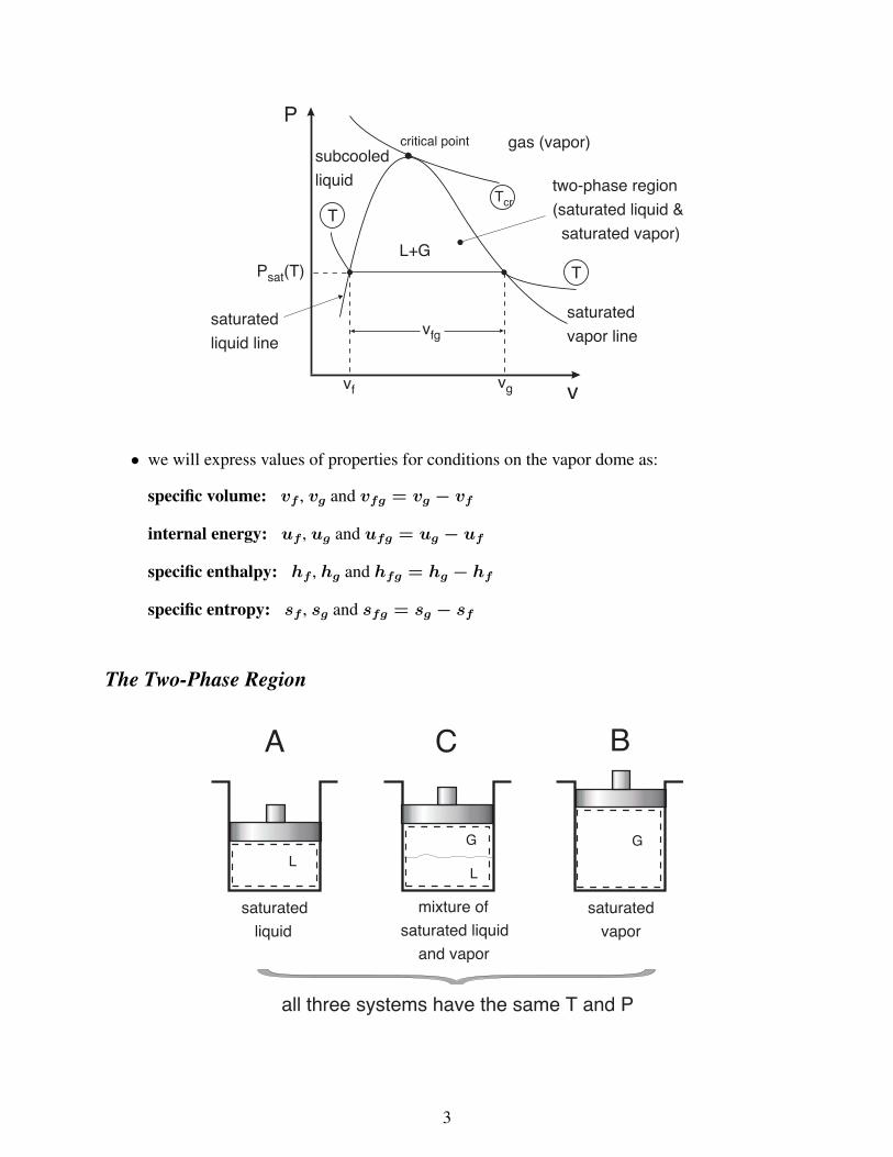
v

critical point

vfg

subcooled

liquid

saturated

liquid line

L+G

vfvg

P

P (T)sat

saturated

vapor line

gas (vapor)

two-phase region

(saturated liquid &

saturated vapor)

Tcr

T

T

• we will express values of properties for conditions on the vapor dome as:

specific volume: vf , vg and vfg = vg − vf

internal energy: uf , ug and ufg = ug − uf

specific enthalpy: hf , hg and hfg = hg − hf

specific entropy: sf , sg and sfg = sg − sf

The Two-Phase Region

LL

G G

A BC

saturated

liquid

mixture of

saturated liquid

and vapor

saturated

vapor

all three systems have the same T and P

3

Question: How can we describe the mixture? P and T are obviously not enough since they areinter-dependent.

Answer: We must also specify how much of each phase is in the mixture, for instance at C inthe above sketch.

We need to define a new thermodynamic property: Quality≡ x =mg

m=

mg

mg +mf

Properties of Saturated Mixtures

• P and T are not independent in the wet vapor region.To fix the state we require (T, x), (T, v), (P, x) . . .

• all the calculations done in the vapor dome can be performed using Tables.

– in Table A-4, the properties are listed under Temperature

– in Table A-5, the properties are listed under Pressure

v

critical point

vfg

saturated liquid line: x=0

L

G

vfv

mixture

vg

P

P (T)sat

saturated vapor line: x=1

T

T

4

Properties of Superheated Vapor

• superheated means T > Tsat at the prevailing P , eg. water at 100 kPa has a saturationtemperature of Tsat(P ) = 99.63 ◦C.

v

L

L+GG

T

T (P)sat

P

P

P = 100 kPa

state: 200 C and 100 kPao

T = 200 Co

Properties of Sub-cooled (Compressed) Liquid

• sub-cooled liquid means T < Tsat at the prevailing P , eg. water at 20 ◦C and 100 kPahas a saturation temperature of Tsat(P ) = 99.63 ◦C.

v

L L+GG

T

T (P)sat

P

P

P = 100 kPa

state: 20 C and 100 kPao

T = 20 Co

5

Using the “Equation of State” to Calculate the Properties ofGaseous Pure Substances

• since most gases are highly superheated at atmospheric conditions. This means we have touse the superheat tables – but this can be very inconvenient

• a better alternative for gases: use the Equation of State which is a functional relationshipbetween P, v, and T (3 measurable properties)

Ideal Gases

• gases that adhere to a pressure, temperature, volume relationship

Pv = RT or PV = mRT

are referred to as ideal gases

– whereR is the gas constant for the specified gas of interest (R = Ru/M )

Ru = Universal gas constant, ≡ 8.314 kJ/(kmol ·K)

M = molecular wieght (or molar mass) of the gas (see Table A-1))

Reference Values for u, h, s

• values of enthalpy, h and entropy, s listed in the tables are with respect to a datum where wearbitrarily assign the zero value. For instance:

Table A-4, A-5: saturated liquid - the reference for both hf and sf is taken as 0 ◦C. Thisis shown as follows:

uf(@T = 0 ◦C) = 0 kJ/kg

hf(@T = 0 ◦C) = 0 kJ/kg

sf(@T = 0 ◦C) = 0 kJ/kg ·K

Table A-11, A-12, & A-13: saturated R134a - the reference for both hf and sf is taken as−40 ◦C. This is shown as follows:

hf(@T = −40 ◦C) = 0 kJ/kg

hf(@T = −40 ◦C) = 0 kJ/kg

sf(@T = −40 ◦C) = 0 kJ/kg ·K

6

Calculation of the Stored Energy

• for most of our 1st law analyses, we need to calculate ∆E

∆E = ∆U + ∆KE + ∆PE

• for stationary systems, ∆KE = ∆PE = 0

• in general: ∆KE =1

2m(V2

2 − V21) and ∆PE = mg(z2 − z1)

• how do we calculate ∆U?

1. one can often find u1 and u2 in the thermodynamic tables (like those examined for thestates of water).

2. we can also explicitly relate ∆U to ∆T (as a mathematical expression) by using thethermodynamic properties Cp and Cv.

Specific Heats: Ideal Gases

• for any gas whose equation of state is exactly

Pv = RT

• for an ideal gas

Cv =du

dT⇒ Cv = Cv(T ) only

Cp =dh

dT⇒ Cp = Cp(T ) only

R = Cp − Cv

• the calculation of ∆u and ∆h for an ideal gas is given as

∆u = u2 − u1 =∫ 2

1Cv(T ) dT (kJ/kg)

∆h = h2 − h1 =∫ 2

1Cp(T ) dT (kJ/kg)

7

First Law of Thermodynamics

Reading Problems3-1→ 3-6 3-40, 3-495-1→ 5-5 5-9, 5-10, 5-25, 5-29, 5-35, 5-42, 5-616-1→ 6-5 6-17, 6-23, 6-37, 6-52, 6-78, 6-87, 6-152

Control Mass (Closed System)The two underlying conservation equations for performing a thermodynamic analysis on a ClosedSystem or a Control Mass, are:

1. Conservation of Mass, and

2. Conservation of Energy

Conservation of Mass

Conservation of Mass, which states that mass cannot be created or destroyed, is implicitly satisfiedby the definition of a control mass.

Conservation of Energy

The first law of thermodynamics states:

Energy cannot be created or destroyed it can only change forms.

• energy transformation is accomplished through energy transfer as work and/or heat. Workand heat are the forms that energy can take in order to be transferred across the systemboundary.

• the first law leads to the principle of Conservation of Energy where we can stipulate theenergy content of an isolated system is constant.

energy entering − energy leaving = change of energy within the system

1

Sign Convention

There are many potential sign conventions that can be used.

Cengel Approach

Heat Transfer: heat transfer to a system is positive and heat transfer from a system is negative.

Work Transfer: work done by a system is positive and work done on a system is negative.

Culham Approach

Anything directed into the system is positive, anything directed out of the system is negative.

Forms of Energy Transfer

Work Versus Heat• Work is macroscopically organized energy transfer.

• Heat is microscopically disorganized energy transfer.

2

Heat Energy• heat is defined as a form of energy that is transferred solely due to a temperature difference

(without mass transfer)

• Notation:

– Q (kJ) amount of heat transfer

– Q (kW ) rate of heat transfer (power)

– q (kJ/kg) - heat transfer per unit mass

– q (kW/kg) - power per unit mass

Work Energy

• work is a form of energy in transit. One should not attribute work to a system.

• Notation:

– W (kJ) amount of work transfer

– W (kW ) power

– w (kJ/kg) - work per unit mass

– w (kW/kg) - power per unit mass

Mechanical Work

• force (which generally varies) times displacement

W12 =∫ 2

1F ds

3

Moving Boundary Work

• consider compression in a piston/cylinder,whereA is the piston cross sectional area (fric-tionless)

• the area under the process curve on a P − Vdiagram is proportional to

∫ 2

1P dV

• sometimes called P dV work orcompression /expansion work

• polytropic processes: where PV n = C

Gravitational Work

Work is defined as force through a distance

W12 =∫ 2

1Fds

Acceleration Work

• if the system is accelerating, the work associated with the change of the velocity can becalculated as follows:

W12 =∫ 2

1F ds =

∫ 2

1ma ds =

∫ 2

1mdVdt

ds =∫ 2

1m dV

ds

dt︸︷︷︸V

and we can then write

W12 =∫ 2

1mV dV = m

(V2

2

2−V2

1

2

)

4

Charge Transfer Work (Electrical Work)

• charge is a conserved quantity, like mass and energy

• the electrical work done is given as

We =∫ 2

1ε I dt

= ε I∆t

Control Volume (Open System)The major difference between a Control Mass and and Control Volume is that mass crosses thesystem boundary of a control volume. We will define a region in space that may be moving orchanging shape. As the process proceeds we will monitor the volume as mass, heat and work crossthe system boundary. The control volume approach will be used for many engineering problemswhere a mass flow rate is present, such as:

• turbines, pumps and compressors

• heat exchangers

• nozzles and diffusers, etc.

CONSERVATION OF MASS:

m

mIN

OUT

mcv

cv

5

rate of increaseof mass within

the CV

=

net rate ofmass flow

IN

−net rate ofmass flowOUT

d

dt(mCV ) = mIN − mOUT

where:

mCV =∫Vρ dV

mIN = (ρ V A)IN

mOUT = (ρ V A)OUT

with V = average velocity

CONSERVATION OF ENERGY:

The 1st law states:

ECV (t) + δQ+ δWshaft + (∆EIN −∆EOUT )+

(δWIN − δWOUT ) = ECV (t+ ∆t) (1)

6

where:

∆EIN = eIN∆mIN

∆EOUT = eOUT∆mOUT

δW = flow work

e =E

m= u︸︷︷︸

internal

+V2

2︸︷︷︸kinetic

+ gz︸︷︷︸potential

Some Practical Assumptions for Control Volumes

Steady State Process: The properties of the material inside the control volume do not changewith time. For example

P1 P

2

P > P2 1

V < V2 1

Diffuser: P changes inside the control volume, butthe pressure at each point does not change withtime.

Steady Flow Process: The properties of the material crossing the control surface do not changewith time. For example

y

x

T = T(y)

T ≠ T(t)

Inlet Pipe: T at the inlet may be different at differ-ent locations, but temperature at each boundarypoint does not change with time.

The steadiness refers to variation with respect to time

• if the process is not steady, it is unsteady or transient

• often steady flow implies both steady flow and steady state

7

Uniform State Process: The properties of the material inside the control volume are uniform andmay change with time. For example

50 Co

50 Co

50 Co

50 Co

60 Co

60 Co

60 Co

60 Co

Q

t=0

t=10

Heating Copper: Cu conducts heat well, so that itheats evenly.

Uniform Flow Process: The properties of the material crossing the control surface are spatiallyuniform and may change with time. For example

y

x

P ≠ P(y)Inlet Pipe: P at the inlet is uniform

across y.

Uniformity is a concept related to the spatial distribution. If the flow field in a process is notuniform, it is distributed.

8

Entropy and the Second Law of Thermodynamics

Reading Problems7-1→ 7-3 8-29, 8-40, 8-43, 8-58, 8-68,7-6→ 7-10 8-99, 8-116, 8-148, 8-149, 8-166,8-1→ 8-13 8-183, 8-189

Introduction

Zeroth Law: led to the concept of temperature

First Law: led to the thermodynamic property called internal energy

Second Law: leads to the thermodynamic property called entropy

Why do we need another law in thermodynamics?

Answer: While the 1st law allowed us to determine the quantity of energy transfer in a processit does not provide any information about the direction of energy transfer nor the quality ofthe energy transferred in the process. In addition, we can not determine from the 1st lawalone whether the process is possible or not. The second law will provide answers to theseunanswered questions.

A process will not occur unless it satisfies both the first and the second laws of thermody-namics.

gasgas

possible

impossible

1: cold system

propeller &

gas rotating

2: warm system

propeller &

gas stationary

1

Second Law of Thermodynamics

The second law of thermodynamics states:

The entropy of an isolated system can never decrease. When an isolated systemreaches equilibrium, its entropy attains the maximum value possible under theconstraints of the system

Definition

Unlike mass and energy, entropy can be produced but it can never be destroyed. That is, the entropyof a system plus its surroundings (i.e. an isolated system) can never decrease (2nd law).

Pm = m2 −m1 = 0 (conservation of mass)

PE = E2 − E1 = 0 (conservation of energy)→ 1st law

PS = Sgen = S2 − S1 ≥ 0 → 2nd law

System

Surroundings

Work

Heat

Non-Isolated Systems

- their entropy may decrease

Isolated System

- its entropy may

never decrease

The second law states, for an isolated system:

(∆S)system + (∆S)surr. ≥ 0

where ∆ ≡ final− initial

2

2nd Law Analysis for a Closed System (Control Mass)

MER TER

CM

dWdQ

TTER

We can first perform a 1st law energy balance on the system shown above.

dU = δQ+ δW (1)

For a simple compressible system

δW = −PdV (2)

From Gibb’s equation we know

TTER dS = dU + PdV (3)

Combining (1), (2) and (3) we get

TTER dS = δQ

where

net in-flow dS =δQ

TTER

net out-flow dS = −δQ

TTER

3

Therefore

(dS)CM︸ ︷︷ ︸≡ storage

=δQ

TTER︸ ︷︷ ︸≡ entropy flow

+ dSgen︸ ︷︷ ︸≡ production

Integrating gives

(S2 − S1)CM =Q1−2

TTER+ Sgen︸ ︷︷ ︸≥0

where

Q1−2

TTER- the entropy associated with heat transfer across a

finite temperature difference, i.e. T > 0

4

2nd Law Analysis for Open Systems (Control Volume)

TER

TER

MER

AA

B

B

FR

FR

CV

S= s m

S= -s m

B

A

1-2

1-2

1-2

1-2

1-2

1-2

1-2

1-2

1-2

B

A

A

B

A

B

B

A

A

B

S= - Qd

S= Qd

T

T

TER

TER

dQ

dQm

m

SCVdW

S=0

isolated S 0gen ≥

where:

FR - fluid reservoirTER - thermal energy reservoirMER - mechanical energy reservoir

5

For the isolated system going through a process from 1→ 2

δSgen = (∆S)sys + (∆S)sur

δSgen = ∆SCV︸ ︷︷ ︸system

+

(−sAmA

1−2 + sBmB1−2 −

δQA1−2

TATER+δQB

1−2

TBTER

)︸ ︷︷ ︸

surroundings

or as a rate equation

Sgen =

(dS

dt

)CV

+

sm+Q

TTER

OUT

−

sm+Q

TTER

IN

This can be thought of as

generation = accumulation+ OUT − IN

Reversible Process

Example: Slow adiabatic compression of a gas

A process 1 → 2 is said to be reversible if the reverse process 2 → 1 restores the system to itsoriginal state without leaving any change in either the system or its surroundings.

→ idealization where S2 = S1 ⇒ Sgen = 0

6

Reversible Compression and Expansion

real or ideal

gas

dQdW

m

W1−2 = −m∫ 2

1Pdv

or on a per unit mass basis

w1−2 =W1−2

m= −

∫ 2

1Pdv

Reversible Isothermal Expansion for an Ideal Gas

The work done at the boundary of a simple, compressible substance (S.C.S.) during a reversibleprocess

w1−2 = −∫ 2

1Pdv = −constant

∫ 2

1

dv

v

= −P1v1 lnv2

v1

= P1v1 lnv1

v2

w1−2 = RT lnv1

v2

= RT lnV1

V2

= RT lnP2

P1

7

Calculation of ∆s in Processes• T − s and h− s (Mollier) diagrams are very useful

– the area under the curve on a T −s diagram is the heat transfer for internally reversibleprocesses

qint,rev =∫ 2

1T ds and qint,rev,isothermal = T∆s

T

s

dA = T ds

process path

1

2

ds

Tabulated Calculation of ∆s for Pure Substances

Depending on the phase of the substance:

Calculation of the Properties of Wet Vapor:

Use Tables A-4 and A-5 to find sf , sg and/or sfg for the following

s = (1− x)sf + xsg s = sf + xsfg

Calculation of the Properties of Superheated Vapor:

Given two properties or the state, such as temperature and pressure, use Table A-6.

Calculation of the Properties of a Compressed Liquid:

Use Table A-7. In the absence of compressed liquid data for a property sT,P ≈ sf@T

8

Calculation of ∆s for Incompressible Materials

ds =du

T= C

dT

T

s2 − s1 =∫ 2

1C(T )

dT

T

∆s = Cavg lnT2

T1

where Cavg = [C(T1) + C(T2)]/2

- if the process is isentropic, then T2 = T1, and ∆s = 0

Calculation of ∆s for Ideal Gases

There are 3 forms of a change in entropy as a function of T & v, T & P , and P & v.

s2 − s1 = Cv lnT2

T1

+R lnv2

v1

= Cp lnT2

T1

−R lnP2

P1

= Cp lnv2

v1

+ Cv lnP2

P1

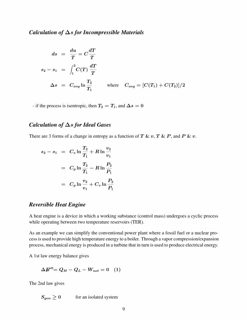
Reversible Heat Engine

A heat engine is a device in which a working substance (control mass) undergoes a cyclic processwhile operating between two temperature reservoirs (TER).

As an example we can simplify the conventional power plant where a fossil fuel or a nuclear pro-cess is used to provide high temperature energy to a boiler. Through a vapor compression/expansionprocess, mechanical energy is produced in a turbine that in turn is used to produce electrical energy.

A 1st law energy balance gives

∆E↗0= QH −QL −Wnet = 0 (1)

The 2nd law gives

Sgen ≥ 0 for an isolated system

9

combustion

gases

cooling

water

boiler

condenser

WP

WT

QH

QH

QL

QL

TER

TER

TH

TL

Wnet

heat

engines

isolated systems

S 0gen ≥

An entropy balance gives

Sgen = (∆S)CM︸ ︷︷ ︸≡0 (cyclic)

+ (∆S)TER−H︸ ︷︷ ︸≡−QH/TH

+ (∆S)TER−L︸ ︷︷ ︸≡+QL/TL

+(∆S)MER↗0

Therefore

QL

TL=QH

TH+ Sgen

or

QL

QH

=TL

TH+Sgen TL

QH

(2)

Combining Eqs. (1) and (2)

Wnet = QH

(1−

TL

TH

)︸ ︷︷ ︸Wmax possible

− TLSgen︸ ︷︷ ︸Wlost due to irreversibilties

The engine efficiency is defined as the benefit over the cost

η =benefit

cost=Wnet

QH

= 1−TL

TH−TLSgen

QH

10

The Carnot Cycle

• an ideal theoretical cycle that is the most efficient conceivable

• based on a fully reversible heat engine - it does not include any of the irreversibilities asso-ciated with friction, viscous flow, etc.

• in practice the thermal efficiency of real world heat engines are about half that of the ideal,Carnot cycle

T

T

T

s s s

Q

Q

Q

W

P = P

P = P

H

H

L

L

1

1

2

4

4

3

in

out

11

Conduction Heat Transfer

Reading Problems10-1→ 10-6 10-38, 10-48, 10-57, 10-70, 10-71, 10-78, 10-92

10-117, 10-121, 10-15311-1→ 11-2 11-14, 11-19, 11-39, 11-45, 11-53, 11-91

Fourier Law of Heat Conduction

x=0

xx

x+ xD

x=Linsulated

Qx

Qx+ xD

gA

∂

∂x

(k∂T

∂x

)︸ ︷︷ ︸

longitudinalconduction

+ g︸︷︷︸internal

heatgeneration

= ρC∂T

∂t︸ ︷︷ ︸thermalinertia

Special Cases1. Multidimensional Systems: The general conduction equation can be extended to three dimen-

sional Cartesian systems as follows:

∂

∂x

(k∂T

∂x

)+

∂

∂y

(k∂T

∂y

)+

∂

∂z

(k∂T

∂z

)+ g = ρC

∂T

∂t

2. Constant Properties: If we assume that properties are independent of temperature, then theconductivity can be taken outside the derivative

1

k

(∂2T

∂x2+∂2T

∂y2+∂2T

∂z2

)+ g = ρC

∂T

∂t

∇2T +g

k=

1

α

∂T

∂t

where

∇ = del operator ≡(∂

∂x+

∂

∂y+

∂

∂z

)

α = thermal diffusivity ≡k

ρC

3. Steady State: If t→∞ then all terms∂

∂t→ 0

∇2T = −g

k⇐ Poisson’s Equation

4. No Internal Heat Generation:

∇2T = 0 ⇐ Laplace’s Equation

2

Thermal Resistance Networks

Resistances in Series

Conditions for 1-D heat flow through a plane wall include:

• constant cross sectional area,A

• steady flow conditions

The total heat flow across the system can be written as

Q =T∞1 − T∞2

Rtotal

where Rtotal =4∑i=1

Ri

The heat flow rate is sometimes written in terms of an overall heat transfer coefficient, U

Q = UA(T∞1 − T∞2)

where

UA =1

Rtotal

=1

1

h1A+

L2

k2A+

L3

k3A+

1

h4A

3

Resistances in Parallel

T1

Q1

T2

Q2

L

R1

k2

k1

R2

For systems of parallel flow paths as shown above, we can use the 1st law to preserve the totalenergy

Q = Q1 + Q2

In general, for parallel networks we can use a parallel resistor network as follows:

T1

T1

T2 T

2

R1

RtotalR

2

R3

=

where

1

Rtotal

=1

R1

+1

R2

+1

R3

+ · · ·

and

Q =T1 − T2

Rtotal

4

Thermal Contact Resistance

• heat flow through the contact turns to seek out the solid-solid contact points, leading to anincrease in resistance and a temperature drop across the interface

Qtotal = Qcontact + Qgap

• the total heat flow rate can be written as

Qtotal = hcA∆Tinterface

where:hc = thermal contact conductanceA = apparent or project area of the contact∆Tinterface = average temperature drop across the interface

The conductance can be written in terms of a resistance as

hcA =Qtotal

∆T=

1

Rc

where:

Rc = contact resistance (K/W )

Table 10-2 can be used to obtain some representative values for contact conductance.

5

Cylindrical Systems

L

r1

r2

Qr

T1

T2

A=2 rLp

k

r

Performing a 1st law energy balance on a control mass from the annular ring of the cylindricalcylinder

dr

r

Qr

Qr + drdQr

dr

C.M.

leads to the following equation

Qr =T1 − T2(

ln(r2/r1)

2πkL

) where R =

(ln(r2/r1)

2πkL

)

Composite Cylinders

Then the total resistance can be written as

Rtotal = R1 +R2 +R3 +R4

6

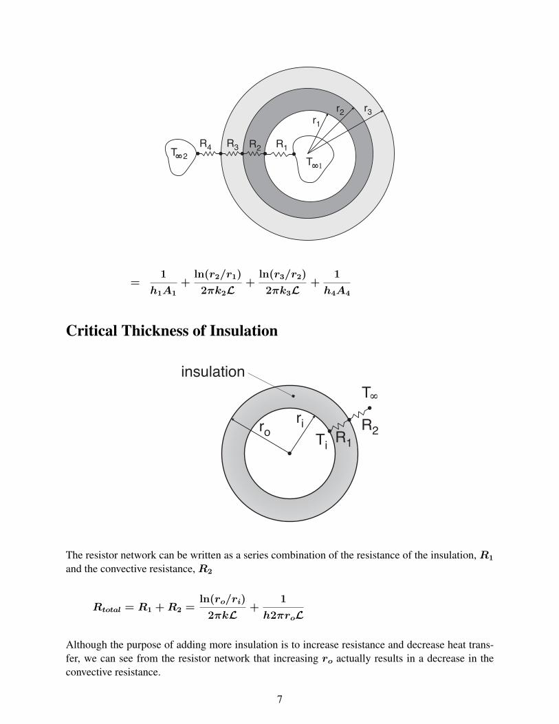
=1

h1A1

+ln(r2/r1)

2πk2L+

ln(r3/r2)

2πk3L+

1

h4A4

Critical Thickness of Insulation

The resistor network can be written as a series combination of the resistance of the insulation, R1

and the convective resistance,R2

Rtotal = R1 +R2 =ln(ro/ri)

2πkL+

1

h2πroL

Although the purpose of adding more insulation is to increase resistance and decrease heat trans-fer, we can see from the resistor network that increasing ro actually results in a decrease in theconvective resistance.

7

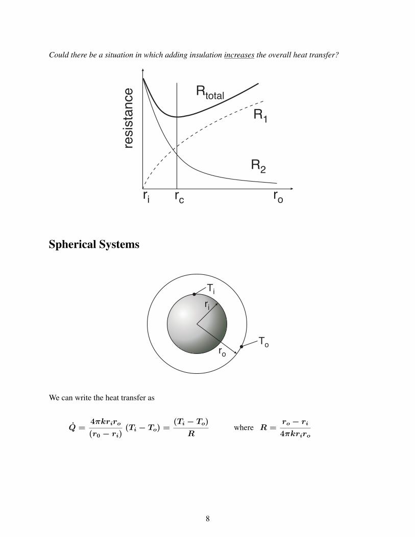
Could there be a situation in which adding insulation increases the overall heat transfer?

Spherical Systems

ri

ro

Ti

To

We can write the heat transfer as

Q =4πkriro

(r0 − ri)(Ti − To) =

(Ti − To)R

where R =ro − ri4πkriro

8

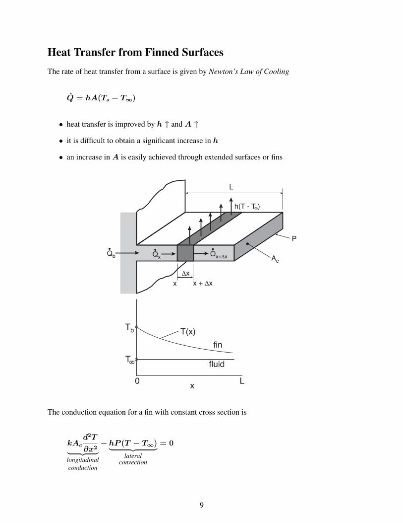
Heat Transfer from Finned SurfacesThe rate of heat transfer from a surface is given by Newton’s Law of Cooling

Q = hA(Ts − T∞)

• heat transfer is improved by h ↑ andA ↑

• it is difficult to obtain a significant increase in h

• an increase inA is easily achieved through extended surfaces or fins

The conduction equation for a fin with constant cross section is

kAc

d2T

∂x2︸ ︷︷ ︸longitudinalconduction

−hP (T − T∞)︸ ︷︷ ︸lateral

convection

= 0

9

The temperature difference between the fin and the surroundings (temperature excess) is usuallyexpressed as

θ = T (x)− T∞

which allows the 1-D fin equation to be written as

d2θ

dx2−m2θ = 0

where the fin parameterm is

m =

(hP

kAc

)1/2

The solution to the differential equation for θ is

θ(x) = C1 sinh(mx) + C2 cosh(mx)

The heat transfer flowing through the base of the fin can be determined as

Qb = Ac

(−k

dT

dx

)@x=0

= θb(kAchP )1/2 tanh(mL)

Transient Heat Conduction

TH − TsTs − T∞

=L/(k ·A)

1/(h ·A)=

internal resistance to H.T.external resistance to H.T.

=hL

k= Bi ≡ Biot number

10

Rint << Rext: the Biot number is small and we can conclude

TH − Ts << Ts − T∞ and in the limit TH ≈ Ts

Rext << Rint: the Biot number is large and we can conclude

Ts − T∞ << TH − Ts and in the limit Ts ≈ T∞

Lumped System Analysis• if the internal temperature of a body remains relatively constant with respect to time

– can be treated as a lumped system analysis

– heat transfer is a function of time only, T = T (t)

• typical criteria for lumped system analysis→ Bi ≤ 0.1

The characteristic length for the 3-D object is given asL = V/A. Other characteristic lengths forconventional bodies include:

SlabV

As

=WH2L

2WH= L

RodV

As

=πr2

oL

2πr0L=r0

2

SphereV

As

=4/3πr3

o

4πr20

=r0

3

At t > 0, T = T (x, y, z, t), however, whenBi < 0.1 then we can assume T ≈ T (t).

11

For an incompressible substance specific heat is constant and we can write

mC︸ ︷︷ ︸≡Cth

dT

dt= − Ah︸︷︷︸

1/Rth

(T − T∞)

where Cth = lumped capacitance

This type of an approach is only valid forBi =hV

kA< 0.1

T (t)− T∞Ti − T∞

= e−t/(Rth·Cth) = e−t/τ = e−bt

where

1

b= τ = Rth · Cth = thermal time constant =

mC

Ah

12

Heisler Charts

The lumped system analysis can be used ifBi = hL/k < 0.1 but what ifBi > 0.1

• need to solve the partial differential equation for temperature

• leads to an infinite series solution⇒ difficult to obtain a solution

The solution procedure for temperature is a function of several parameters

T (x, t) = f(x, L, t, k, α, h, Ti, T∞)

We must find a solution to the PDE

∂2T

∂x2=

1

α

∂T

∂t

The analytical solution to this equation takes the form of a series solution

T (x, t)− T∞Ti − T∞

=∞∑

n=1,3,5...

Ane

(−nλ

L

)2

αt

cos

(nλx

L

)

If we let Fo = αt/L2, we can see that the first term with n = 1 provides a very good estimateto the infinite series solution.

By using dimensionless groups, we can reduce the temperature dependence to 3 dimensionlessparameters

Dimensionless Group Formulation

temperature θ(x, t) =T (x, t)− T∞Ti − T∞

position x = x/L

heat transfer Bi = hL/k Biot number

time Fo = αt/L2 Fourier number

13

note: Cengel uses τ instead of Fo.

Now we can write

θ(x, t) = f(x,Bi, Fo)

The characteristic length for the Biot number is

slab L = Lcylinder L = rosphere L = ro

contrast this versus the characteristic length for the lumped system analysis.

With this, two approaches are possible

1. use the first term of the infinite series solution. This method is only valid for Fo > 0.2

2. use the Heisler charts for each geometry as shown in Figs. 11-15, 11-16 and 11-17

First term solution: Fo > 0.2→ error about 2% max.

Plane Wall: θwall(x, t) =T (x, t)− T∞Ti − T∞

= A1e−λ2

1Fo cos(λ1x/L)

Cylinder: θcyl(r, t) =T (r, t)− T∞Ti − T∞

= A1e−λ2

1Fo J0(λ1r/ro)

Sphere: θsph(r, t) =T (r, t)− T∞Ti − T∞

= A1e−λ2

1Fosin(λ1r/ro)

λ1r/ro

where λ1, A1 can be determined from Table 18-1 based on the calculated value of the Biot number(will likely require some interpolation).

14

Convection Heat Transfer

Reading Problems12-1→ 12-8 12-41, 12-46, 12-53, 12-57, 12-76, 12-8113-1→ 13-6 13-39, 13-47, 13-5914-1→ 14-4 14-24, 14-29, 14-47, 14-60

Introduction

• convection heat transfer is the transport mechanism made possible through the motion offluid

• the controlling equation for convection is Newton’s Law of Cooling

Qconv =∆T

Rconv

= hA(Tw − T∞) ⇒ Rconv =1

hA

where

A = total convective area, m2

h = heat transfer coefficient, W/(m2 ·K)

1

Tw = surface temperature, ◦C

T∞ = fluid temperature, ◦C

Factors Affecting Convective Heat Transfer

Geometry: flat plate, circular cylinder, sphere, spheroids plus many other shapes. In addi-tion to the general shape, size, aspect ratio (thin or thick) and orientation (vertical orhorizontal) play a significant role in convective heat transfer.

Type of flow: forced, natural, mixed convection as well as laminar, turbulent and transi-tional flows. These flows can also be considered as developing, fully developed, steadyor transient.

Boundary condition: (i) isothermal wall (Tw = constant) or(ii) isoflux wall (qw = constant)

Type of fluid: viscous oil, water, gases (air) or liquid metals.

Fluid properties: symbols and units

mass density : ρ, (kg/m3)

specific heat capacity : Cp, (J/kg ·K)

dynamic viscosity : µ, (N · s/m2)

kinematic viscosity : ν, ≡ µ/ρ (m2/s)

thermal conductivity : k, (W/m ·K)

thermal diffusivity : α, ≡ k/(ρ · Cp) (m2/s)

Prandtl number : Pr, ≡ ν/α (−−)

volumetric compressibility : β, (1/K)

All properties are temperature dependent and are usually determined at the film tem-perature, Tf = (Tw + T∞)/2

External Flow: the flow engulfs the body with which it interacts thermally

Internal Flow: the heat transfer surface surrounds and guides the convective stream

Forced Convection: flow is induced by an external source such as a pump, compressor, fan, etc.

2

Natural Convection: flow is induced by natural means without the assistance of an externalmechanism. The flow is initiated by a change in the density of fluids incurred as a resultof heating.

Mixed Convection: combined forced and natural convection

Dimensionless Groups

In the study and analysis of convection processes it is common practice to reduce the total numberof functional variables by forming dimensionless groups consisting of relevant thermophysicalproperties, geometry, boundary and flow conditions.

Prandtl number: Pr = ν/α where 0 < Pr < ∞ (Pr → 0 for liquid metals and Pr →∞ for viscous oils). A measure of ratio between the diffusion of momentum to the diffusionof heat.

Reynolds number: Re = ρUL/µ ≡ UL/ν (forced convection). A measure of the balancebetween the inertial forces and the viscous forces.

Peclet number: Pe = UL/α ≡ RePr

Grashof number: Gr = gβ(Tw − Tf)L3/ν2 (natural convection)

Rayleigh number: Ra = gβ(Tw − Tf)L3/(α · ν) ≡ GrPr

Nusselt number: Nu = hL/kf This can be considered as the dimensionless heat transfercoefficient.

Stanton number: St = h/(UρCp) ≡ Nu/(RePr)

Forced ConvectionThe simplest forced convection configuration to consider is the flow of mass and heat near a flatplate as shown below.

• as Reynolds number increases the flow has a tendency to become more chaotic resulting indisordered motion known as turbulent flow

– transition from laminar to turbulent is called the critical Reynolds number,Recr

Recr =U∞xcr

ν

3

– for flow over a flat plateRecr ≈ 500, 000

• the thin layer immediately adjacent to the wall where viscous effects dominate is known asthe laminar sublayer

Boundary Layers

Velocity Boundary Layer

• the region of fluid flow over the plate where viscous effects dominate is called the velocityor hydrodynamic boundary layer

Thermal Boundary Layer

• the thermal boundary layer is arbitrarily selected as the locus of points where

T − TwT∞ − Tw

= 0.99

4

Flow Over Plates

1. Laminar Boundary Layer Flow, Isothermal (UWT)

The local values of the skin friction and the Nusselt number are given as

Cf,x =0.664

Re1/2x

Nux = 0.332Re1/2x Pr1/3 ⇒ local, laminar, UWT, Pr ≥ 0.6

NuL =hLL

kf= 0.664 Re

1/2L Pr1/3 ⇒ average, laminar, UWT, Pr ≥ 0.6

For low Prandtl numbers, i.e. liquid metals

Nux = 0.565Re1/2x Pr1/2 ⇒ local, laminar, UWT, Pr ≤ 0.6

2. Turbulent Boundary Layer Flow, Isothermal (UWT)

Cf,x =τw

(1/2)ρU2∞

=0.0592

Re0.2x

⇒ local, turbulent, UWT, Pr ≥ 0.6

Nux = 0.0296Re0.8x Pr1/3 ⇒

local, turbulent, UWT,0.6 < Pr < 100, Rex > 500, 000

5

NuL = 0.037Re0.8L Pr1/3 ⇒

average, turbulent, UWT,0.6 < Pr < 100, Rex > 500, 000

3. Combined Laminar and Turbulent Boundary Layer Flow, Isothermal (UWT)

NuL =hLL

k= (0.037Re0.8

L − 871) Pr1/3 ⇒

average, combined, UWT,0.6 < Pr < 60,500, 000 ≤ ReL > 107

4. Laminar Boundary Layer Flow, Isoflux (UWF)

Nux = 0.453Re1/2x Pr1/3 ⇒ local, laminar, UWF, Pr ≥ 0.6

5. Turbulent Boundary Layer Flow, Isoflux (UWF)

Nux = 0.0308Re4/5x Pr1/3 ⇒ local, turbulent, UWF, Pr ≥ 0.6

Flow Over Cylinders and Spheres

1. Boundary Layer Flow Over Circular Cylinders, Isothermal (UWT)

The Churchill-Berstein (1977) correlation for the average Nusselt number for long (L/D > 100)cylinders is

NuD = S∗D + f(Pr)Re1/2D

1 +

(ReD

282, 000

)5/84/5

⇒average, UWT, Re < 107

0 ≤ Pr ≤ ∞, Re · Pr > 0.2

where S∗D is the diffusive term associated withReD → 0 and is given as

S∗D = 0.3

and the Prandtl number function is

f(Pr) =0.62 Pr1/3

[1 + (0.4/Pr)2/3]1/4

6

All fluid properties are evaluated at Tf = (Tw + T∞)/2.

2. Boundary Layer Flow Over Non-Circular Cylinders, Isothermal (UWT)

The empirical formulations of Zhukauskas and Jakob given in Table 12-3 are commonly used,where

NuD ≈hD

k= C RemD Pr

1/3 ⇒ see Table 12-3 for conditions

3. Boundary Layer Flow Over a Sphere, Isothermal (UWT)

For flow over an isothermal sphere of diameterD

NuD = S∗D +[0.4Re

1/2D + 0.06Re

2/3D

]Pr0.4

(µ∞

µw

)1/4

⇒

average, UWT,0.7 ≤ Pr ≤ 380

3.5 < ReD < 80, 000

where the diffusive term atReD → 0 is

S∗D = 2

and the dynamic viscosity of the fluid in the bulk flow, µ∞ is based on T∞ and the dynamicviscosity of the fluid at the surface, µw, is based on Tw. All other properties are based on T∞.

7

Internal Flow

The Reynolds number is given as

ReD =UmD

ν

For flow in a tube:

ReD < 2300 laminar flow

2300 < ReD < 4000 transition to turbulent flow

ReD > 4000 turbulent flow

Hydrodynamic (Velocity) Boundary Layer

• the hydrodynamic boundary layer thickness can be approximated as

δ(x) ≈ 5x

(Umx

ν

)−1/2

=5x√Rex

• the hydrodynamic entry length can be approximated as

Lh ≈ 0.05ReDD (laminar flow)

8

Thermal Boundary Layer

• the thermal entry length can be approximated as

Lt ≈ 0.05ReDPrD (laminar flow)

• for turbulent flow Lh ≈ Lt ≈ 10D

Wall Boundary Conditions

1. Uniform Wall Heat Flux: Since the wall flux qw is uniform, the local mean temperature de-noted as

Tm,x = Tm,i +qwA

mCp

will increase in a linear manner with respect to x.

The surface temperature can be determined from

Tw = Tm +qw

h

9

2. Isothermal Wall: The outlet temperature of the tube is

Tout = Tw − (Tw − Tin) exp[−hA/(mCp)]

Because of the exponential temperature decay within the tube, it is common to present themean temperature from inlet to outlet as a log mean temperature difference where

Q = hA∆Tln

∆Tln =Tout − Tin

ln

(Tw − ToutTw − Tin

) =Tout − Tin

ln(∆Tout/∆Tin)

10

1. Laminar Flow in Circular Tubes, Isothermal (UWT) and Isoflux (UWF)

For laminar flow whereReD ≤ 2300

NuD = 3.66 ⇒ fully developed, laminar, UWT, L > Lt & Lh

NuD = 4.36 ⇒ fully developed, laminar, UWF, L > Lt & Lh

NuD = 1.86

(ReDPrD

L

)1/3 ( µbµw

)0.14

⇒

developing laminar flow, UWT,Pr > 0.5

L < Lh or L < Lt

In all cases the fluid properties are evaluated at the mean fluid temperature given as

Tmean =1

2(Tm,in + Tm,out)

except for µw which is evaluated at the wall temperature, Tw.

2. Turbulent Flow in Circular Tubes, Isothermal (UWT) and Isoflux (UWF)

For turbulent flow whereReD ≥ 2300 the Dittus-Bouler equation (Eq. 13-68) can be used

NuD = 0.023Re0.8D Prn ⇒

turbulent flow, UWT or UWF,0.7 ≤ Pr ≤ 160

ReD > 2, 300

n = 0.4 heatingn = 0.3 cooling

For non-circular tubes, again we can use the hydraulic diameter,Dh = 4Ac/P to determine boththe Reynolds and the Nusselt numbers.

In all cases the fluid properties are evaluated at the mean fluid temperature given as

Tmean =1

2(Tm,in + Tm,out)

11

Natural Convection

What Drives Natural Convection?• fluid flow is driven by the effects of buoyancy

• fluids tend to expand when heated and contract when cooled at constant pressure

• therefore a fluid layer adjacent to a surface will become lighter if heated and heavier if cooledby the surface

Recall from forced convection that the flow behavior is determined by the Reynolds number. Innatural convection, we do not have a Reynolds number but we have an analogous dimensionlessgroup called the Grashof number

Gr =buouancy forceviscous force

=gβ(Tw − T∞)L3

ν2

where

g = gravitational acceleration,m/s2

12

β = volumetric expansion coefficient, β ≡ 1/T

Tw = wall temperature,K

T∞ = ambient temperature,K

L = characteristic length,m

ν = kinematic viscosity,m2/s

The volumetric expansion coefficient, β, is used to express the variation of density of the fluid withrespect to temperature and is given as

β = −1

ρ

(∂ρ

∂T

)P

Natural Convection Over Surfaces

• the velocity and temperature profiles within a boundary layer formed on a vertical plate in astationary fluid looks as follows:

13

• note that unlike forced convection, the velocity at the edge of the boundary layer goes to zero

Natural Convection Heat Transfer Correlations

The general form of the Nusselt number for natural convection is as follows:

Nu = f(Gr, Pr) ≡ CGrmPrn where Ra = Gr · Pr

1. Laminar Flow Over a Vertical Plate, Isothermal (UWT)

The general form of the Nusselt number is given as

NuL =hLkf

= C

gβ(Tw − T∞)L3

ν2︸ ︷︷ ︸≡Gr

1/4 ν

α︸︷︷︸≡Pr

1/4

= C Gr1/4L Pr1/4︸ ︷︷ ︸Ra1/4

where

RaL = GrLPr =gβ(Tw − T∞)L3

αν

2. Laminar Flow Over a Long Horizontal Circular Cylinder, Isothermal (UWT)

The general boundary layer correlation is

NuD =hD

kf= C

gβ(Tw − T∞)D3

ν2︸ ︷︷ ︸≡Gr

1/4 ν

α︸︷︷︸≡Pr

1/4

= C Gr1/4D Pr1/4︸ ︷︷ ︸Ra

1/4D

where

RaD = GrDPr =gβ(Tw − T∞)L3

αν

All fluid properties are evaluated at the film temperature, Tf = (Tw + T∞)/2.

14

Natural Convection From Plate Fin Heat Sinks

Plate fin heat sinks are often used in natural convection to increase the heat transfer surface areaand in turn reduce the boundary layer resistance

R ↓=1

hA ↑

For a given baseplate area,W ×L, two factors must be considered in the selection of the numberof fins

• more fins results in added surface area and reduced boundary layer resistance,

R ↓=1

hA ↑

• more fins results in a decrease fin spacing, S and in turn a decrease in the heat transfercoefficient

R ↑=1

h ↓ A

A basic optimization of the fin spacing can be obtained as follows:

Q = hA(Tw − T∞)

15

where the fins are assumed to be isothermal and the surface area is 2nHL, with the area of the finedges ignored.

For isothermal fins with t < S

Sopt = 2.714

(S3L

RaS

)1/4

= 2.714

(L

Ra1/4L

)

with

RaL =gβ(Tw − T∞)L3

ν2Pr

The corresponding value of the heat transfer coefficient is

h = 1.307k/Sopt

All fluid properties are evaluated at the film temperature.

16

Radiation Heat Transfer

Reading Problems15-1→ 15-7 15-27, 15-33, 15-50, 15-58, 15-77, 15-79,

15-86, 15-106, 15-107

IntroductionRadiation is a photon emission that occurs when electrons change orbit. Thermal radiation occurswhen the excitation is caused by heating.

The following figure shows the relatively narrow band occupied by thermal radiation.

An even narrower band inside the thermal radiation spectrum is denoted as the visible spectrum,that is the thermal radiation that can be seen by the human eye. The visible spectrum occupiesroughly 0.4 − 0.7 µm. Thermal radiation is mostly in the infrared range. As objects heatup, their energy level increases, their frequency, ν, increases and the wavelength of the emittedradiation decreases. That is why objects first become red when heated and eventually turn whiteupon further heating.

1

Blackbody RadiationA blackbody is an ideal radiator that

• absorbs all incident radiation regardless of wavelength and direction

Definitions1. Blackbody emissive power: the radiation emitted by a blackbody per unit time and per

unit surface area

Eb = σ T 4 [W/m2] ⇐ Stefan-Boltzmann law

where

σ = Stefan-Boltzmann constant = 5.67× 10−8 W/(m2 ·K4)

and the temperature T is given inK.

2. Spectral blackbody emissive power: the amount of radiation energy emitted by a black-body per unit surface area and per unit wavelength about the wavelength λ. The followingrelationship between emissive power, temperature and wavelength is known as Plank’s dis-tribution law

Eb,λ =C1

λ5[exp(C2/λT )− 1][W/(m2 · µm)]

where

C0 = 2.998× 108 [m/s] (vacuum conditions)

C1 = 2πhC20 = 3.743× 108 [W · µm4/m2]

C2 = hC0/K = 1.439× 104 [µm ·K]

K = Boltzmann constant ≡ 1.3805× 10−23 [J/K]

h = Plank′s constant ≡ 6.63× 10−34 [J · s]

Eb,λ = energy of radiation in the wavelength

band dλ per unit area and time

2

The wavelength at which the peak emissive power occurs for a given temperature can beobtained from Wien’s displacement law

(λT )max power = 2897.8 µm ·K

3. Blackbody radiation function: the fraction of radiation emitted from a blackbody at tem-perature, T in the wavelength band λ = 0→ λ

f0→λ =

∫ λ0Eb,λ(T ) dλ∫ ∞

0Eb,λ(T ) dλ

=

∫ λ0

C1

λ5[exp(C2/λT )− 1]dλ

σT 4

let t = λT and dt = T dλ, then

f0→λ =

∫ t0

C1T5(1/T )dt

t5[exp(C2/t)− 1]

σT 4

=C1

σ

∫ λT0

dt

t5[exp(C2/t)− 1]

= f(λT )

f0→λ is tabulated as a function λT in Table 15.2

3

We can easily find the fraction of radiation emitted by a blackbody at temperature T over adiscrete wavelength band as

fλ1→λ2 = f(λ2T )− f(λ1T )

fλ→∞ = 1− f0→λ

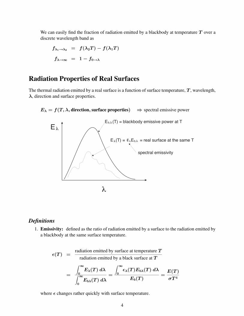
Radiation Properties of Real SurfacesThe thermal radiation emitted by a real surface is a function of surface temperature, T , wavelength,λ, direction and surface properties.

Eλ = f(T, λ, direction, surface properties) ⇒ spectral emissive power

Definitions1. Emissivity: defined as the ratio of radiation emitted by a surface to the radiation emitted by

a blackbody at the same surface temperature.

ε(T ) =radiation emitted by surface at temperature T

radiation emitted by a black surface at T

=

∫ ∞0Eλ(T ) dλ∫ ∞

0Ebλ(T ) dλ

=

∫ ∞0ελ(T )Ebλ(T ) dλ

Eb(T )=E(T )

σT 4

where ε changes rather quickly with surface temperature.

4

2. Diffuse surface: properties are independent of direction.

3. Gray surface: properties are independent of wavelength.

4. Irradiation,G: the radiation energy incident on a surface per unit area and per unit time

If we normalize with respect to the total irradiation

α+ ρ+ τ = 1

5. Radiosity, J : the total radiation energy leaving a surface per unit area and per unit time.

For a surface that is gray and opaque, i.e. ε = α and α+ ρ = 1, the radiosity is given as

J = radiation emitted by the surface + radiation reflected by the surface

= ε Eb + ρG

= εσT 4 + ρG

Since ρ = 0 for a blackbody, the radiosity of a blackbody is

J = σT 4

5

Solar RadiationThe incident radiation energy reaching the earth’s atmosphere is known as the solar constant, Gs

and has a value of

Gs = 1353W/m2

While this value can change by about ±3.4% throughout the year its change is relatively smalland is assumed to be constant for most calculations. AlthoughGs = 1353W/m2 at the edge ofthe earth’s atmosphere, the following figure shows how it is dispersed as it approaches the surfaceof the earth.

View Factor (Shape Factor, Configuration Factor)

• the radiative exchange between surfaces clearly depends on how well the surfaces “see” oneanother. This information is provided by using shape factors (or view factors or configurationfactors).

• Definition: The view factor, Fi→j is defined as the fraction of radiation leaving surface iwhich is intercepted by surface j. Hence

Fi→j =Qi→j

AiJi=

radiation reaching jradiation leaving i

It can be shown that

Fi→j =1

Ai

∫Ai

∫Aj

cos θi cos θj

πR2dAidAj

6

This is purely a geometrical property.

It is also found that

Fj→i =1

Aj

∫Ai

∫Aj

cos θi cos θj

πR2dAidAj

The last two equations show that

AiFi→j = AjFj→i

This is called the reciprocity relation.

• consider an enclosure withN surfaces

Since this is an enclosure, the energy leaving a given surface is intercepted by the remainingsurfaces in proportion to how well they “see” that surface. For example:

A1J1 = Q1→1 + Q1→2 + . . .+ Q1→N

7

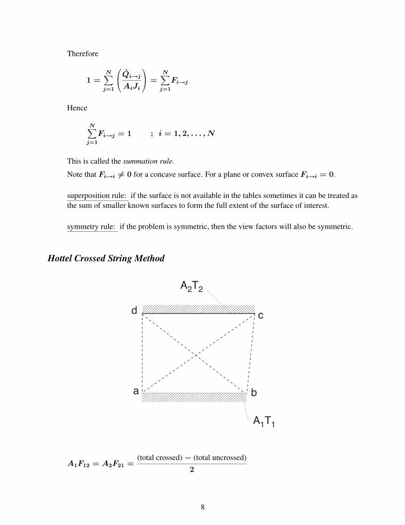
Therefore

1 =N∑j=1

Qi→j

AiJi

=N∑j=1

Fi→j

Hence

N∑j=1

Fi→j = 1 ; i = 1, 2, . . . , N

This is called the summation rule.

Note that Fi→i 6= 0 for a concave surface. For a plane or convex surface Fi→i = 0.

superposition rule: if the surface is not available in the tables sometimes it can be treated asthe sum of smaller known surfaces to form the full extent of the surface of interest.

symmetry rule: if the problem is symmetric, then the view factors will also be symmetric.

Hottel Crossed String Method

A1F12 = A2F21 =(total crossed)− (total uncrossed)

2

8

A1 andA2 do not have to be parallel

A1F12 = A2F21 =1

2[(ac+ bd)︸ ︷︷ ︸

crossed

− (bc+ ad)︸ ︷︷ ︸uncrossed

]

Radiation Exchange Between Diffuse-Gray SurfacesForming an Enclosure

We will assume that:

1. each surface of the enclosure is isothermal

2. radiosity, Ji, and irradiation,Gi are uniform over each surface

3. the surfaces are opaque (τi = 0) and diffuse-gray (αi = εi)

4. the cavity is filled with a fluid which does not participate in the radiative exchange process

• an energy balance on the i′th surface gives:

Qi = qiAi = Ai(Ji −Gi)

Qi = Ai(Ei − αiGi) (1)

Ji = Ei + ρiGi (2)

Ei = εiEb,i = εiσT4i (3)

ρi = 1− αi = 1− εi (4) ⇒ since αi + ρi + τi↗0= 1

and αi = εi

9

Combining Eqs. 2, 3 and 4 gives

Ji = εiEb,i + (1− εi)Gi (5)

Combining this with Eq. 1 gives

Qi =Eb,i − Ji(

1− εiεiAi

) ≡ potential differencesurface resistance

• next consider radiative exchange between the surfaces.

By inspection it is clearly seen that

{irradiation on

surface i

}=

{radiation leaving theremaining surfaces

}

AiGi =N∑j=1

Fj→i(AjJj) =N∑j=1

AiFi→jJi

Therefore

Gi =N∑j=1

Fi→jJj

Combining this with Eq. 5 gives

Ji = εiσT4i + (1− εi)

N∑j=1

Fi→jJj

In addition we can write

Qi = AiJi −N∑j=1

AiFi→jJj

Qi =N∑j=1

Ji − Jj(1

AiFi→j

) ≡ potential differencespace resistance

10