basic tools of linear control theorygrupen/403/slides/403control.pdf · •proposed the...

Basic Tools of Linear Control Theory

Outline

• Spinal Motor Units

• Negative Feedback• Open- and Closed-Loop Control

• The Spring-Mass-Damper

• Lyapunov Stability

• Laplace Transform• the Characteristic Equation• Equilibrium Setpoint Control - A RobotControllerclass exercise - Roger’s eye and PD control

• Frequency-Domain Response DemonstrationRoger’s eye frequency-domain response

1 Copyright c©2019 Roderic Grupen

Motor Circuits

forcelength

cortex

brain stem

tendonorgans

+ − spindlereceptors

innervation

+

−

extrafusal muscle

intrafusal muscle

spinal cord interneurons

−motorneurons

−motorneurons

• α-motor neurons initiate motion—they’re fast

• each will innervate an average of 200 muscle fibers.

• relatively slow γ-motor neuron regulates muscle tone by settingthe reference length of the spindle receptor.

• Golgi tendon organ measures the tension in the tendon andinhibits the α-motor neuron if it exceeds safe levels


Negative Feedback

forcelength

cortex

brain stem

tendonorgans

+ − spindlereceptors

innervation

+

−

extrafusal muscle

intrafusal muscle

spinal cord interneurons

−motorneurons

−motorneurons

• If (spindle length > reference), the α-motor neuron cause acontraction of the muscle tissue

• if (spindle length< reference), the α-motor neuron is inhibited,allowing the muscle to extend

Negative Feedback

...the α-motor neuron changes its output so as to cancel someof its input...


Negative Feedback

• first submitted for a patent in 1928 by Harold S. Black

• it explained the operating principle of many devices includingWatt’s governor that pre-dated it by some 40 years.

• catalyzed the field of cybernetics

• now heralded as the fundamental principle of stability in com-pensated dynamical systems

The Muscle Stretch Reflex

sensorynerve

ventralhorn

motornerve

whitematter

graymatter

spinalnerve

patellertendon

musclespindle

neuromuscular junction

synapse


Open- and Closed-Loop Control

open-loop -a trigger event causes a response without further stimulation

withdrawl reflex

C5

C6

C7C8

T1

median nerve

ulnar nerve

T1

C8

C7

C6

C5

peripheral nerves

radial nerve

dorsalroots

ventralroots

sensorynerve

dorsalfasciculus

ventralhorn motor

nerve

whitematter

graymatter

DORSAL

VENTRAL

free−endednerve fiber

spinalnerve

neuromuscular junction

closed-loop -a (time-varying) setpoint is achieved by constantly measuring andcorrecting in order to actively reject disturbances

Norbert Weiner - cybernetics (helmsman), homeostasis, endocrinesystem


The Spring-Mass-Damper

Fk = −Kx

m

K B

x = 0

Fb = −Bv = −Bx

fd(t)

m

Kx Bx

x

∑

F = mx = f (t)− Bx−Kx

mx + Bx +Kx = f (t), or

x+(B/m)x+(K/m)x = f (t)/m =∼

f (t) “specific” applied force

x + (B/m)x + (K/m)x = 0 the characteristic equation

arbitrary references require a change of variables:

x′(t) = x(t)− xrefx′ = x


The Spring-Mass-Damper

m

K B

x = 0

x + (B/m)x + (K/m)x = 0

we can write this another way:

x + 2ζωnx + ω2nx = 0 harmonic oscillator

where:

ωn =√

K/m [rad/sec] - natural frequency

ζ =B

2√Km

0 ≤ ζ ≤ ∞ - damping ratio


Closed-Loop Control

K B

xM robot

digitalcontrol

Σ

ΣΣ

actx

K B

_+

_+

++

+actx

xref

ref(x = 0)

ref(x = 0)f motor M

robot digitalcontrol

sample and hold ∆t = τwhere 1

τ [Hz] is the servo rateanalog ∆t→ 0

Σ

ΣΣ

K B

_+

_+

++

+ I

Oref

Oact

motorτ

ly

x

m

Oact

Oact

( = 0)Oref

Oref( = 0)

K, B

I = ml 2


Roger MotorUnits.cMaster Control Procedure

/* == the simulator executes control_roger() once ==*/

/* == every simulated 0.001 second (1000 Hz) ==*/

control_roger(roger, time)

Robot * roger;

double time;

{

update_setpoints(roger);

// turn setpoint references into torques

PDController_base(roger, time);

PDController_arms(roger, time);

PDController_eyes(roger, time);

}


Roger MotorUnits.cPDController eyes()

double Kp_eye, Kd_eye;

// gain values set in enter_params()

/* Eyes PD controller:

/* -pi/2 < eyes_setpoint < pi/2 for each eye */

PDController_eyes(roger, time)

Robot * roger;

double time;

{

int i;

double theta_error;

for (i = 0; i < NEYES; i++) {

theta_error = roger->eyes_setpoint[i]

- roger->eye_theta[i];

// roger->eye_torque[i] = ...

}

}


Roger MotorUnits.cPDcontroller arms()

double Kp_arm, Kd_arm;

// gain values set in enter_params()

/* Arms PD controller: -pi < arm_setpoint < pi */

/* for the shoulder and elbow of each arm */

PDController_arms(roger, time)

Robot * roger;

double time;

{

int i;

double theta_error;

for (i = LEFT; i <= RIGHT; ++i) {

theta_error = roger->arm_setpoint[i][0]

- roger->arm_theta[i][0];

// -M_PI < theta_error < +M_PI

// roger->arm_torque[i][0] = ...

// roger->arm_torque[i][1] = ...

}

}


Analytic Stability —Lyapunov’s Second/Direct Method

Stability - the origin of the state space is stable if there existsa region, S(r), such that states which start within S(r) remainwithin S(r).

Asymptotic Stability - a system is asymptotically stable inS(r) if as t → ∞, the system state approaches the origin of thestate space.

x

x

x

x

S(r)


Analytic Stability -Lyapunov’s Second/Direct Method

Define: an arbitrary scalar function, V (x, t), called a Lyapunovfunction, continuous is all first derivatives, where x is the stateand t is time,

Iff: If the function, V (x, t), exists such that:

(a) V (0, t) = 0, and(b) V (x, t) > 0, for x 6= 0 (positive definite), and(c) ∂V/∂t < 0 (negative definite),

Then: the system described by V is asymptotically stable in theneighborhood of the origin.

...if a system is stable, then there exists a suitable Lyapunovfunction.

...if, however, a particular Lyapunov function does not satisfythese criteria, it is not necessarily true that this system isunstable.


EXAMPLE: spring-mass-damper

m

K B

x = 0

system dynamics:

x +B

mx +

K

mx = 0

E =

∫ v

0

(mv)dv +

∫ x

0

(Kx)dx

=1

2mv2 +

1

2Kx2

=1

2mx2 +

1

2Kx2

Lyapunov function:

V (x, t) = E =mx2

2+Kx2

2

(a) V (0, t) = 0,√

(b) V (x, t) > 0,√

(c) ∂V/∂t negative definite?



m

K B

x = 0 Lyapunov function:

V (x, t) = E =mx2

2+Kx2

2

dE

dt= mxx +Kxx

dE

dt= mx [−(B/m)x− (K/m)x] +Kxx

dE

dt= −Bx2

stable? or not stable?



m

K B

x = 0

x

0.40.6

B=0B>0

0.2 t=0

1.00.8

x

...the entire state space is asymptotically stable for B > 0.


Recap: Introduction to Control

So far, we have:

• introduced the concept of negative feedback in robotics andbiology;

• proposed the spring-mass-damper (SMD) as a prototype forproportional-derivative (PD) control;

• we derived the dynamics for the SMD using Newton’s laws anda free body diagram; and

• we introduced Lypunov’s Direct Method to show the the SMD(and thus PD control) is asymptotically stable.

Now: we describe more tools for analyzing closed-loop linear con-trollers — the Laplace transform and transfer functions


Tools: Complex Numbers

Cartesian form: s = σ + jω

• σ = Re(s) is the real part of s

• ω = Im(s) is the imaginary part of s

• j =√−1 (sometimes I may use i)

Polar form: s = rejφ

• r =√σ2 + ω2 is the modulus or magnitude of s

• φ = atan(ω/σ) is the angle or phase of s

• Euler’s formula: ejφ = cos(φ) + jsin(φ)

Therefore, complex exponential of s = σ + jω:

est = e(σ+jω)t = eσtejωt = eσt [cos(ωt) + jsin(ωt)]


Laplace Transform

...so what does this do for us?

if we assume that the robot movements are functions of time f (t),such that

f (t) ∼ est

then, from calculus:

d

dt[f (t)] = f (t) ∼ sest

∫

f (t)dt ∼ 1

sest

let’s say this a different way (ignoring some details about boundaryconditions for now), if L [f (t)] = F (s), then

L[

df

dt

]

= sF (s) , and

L[∫

f (t)dt

]

=1

sF (s)


Laplace TransformDifferential Equations

for example, f + af = 0

i.e. the “slope” of function f (df/dt) is proportional to the valueof the function, df/dt = −af

assuming f (t) ∼ est:

sF (s) + aF (s) = 0

(s + a)F (s) = 0

and the first-order differential equation is transformed intopolynomial (s + a),

root (s = −a) tells us more about function f (t),

f (t) ∼ A0 + A1e−at

where coefficients A0 and A1 are constants that depend onboundary conditions, i.e. if f (0) = 1 and f (∞) = 0

verify that: A0 = 0 and A1 = 1


The Harmonic Oscillator

x + 2ζωnx + ω2nx = 0

L(·)−→

←−L−1(·)

[

s2 + 2ζωns + ω2n

]

X(s) = 0

yields the characteristic equation of the 2nd-order oscillator inthe complex frequency domain

s2 + 2ζωns + ω2n = 0


Roots of the Characteristic Equation

s2 + 2ζωns + ω2n = 0

roots ⇒ values of s in Aest that satisfy the original differentialequation

x + 2ζωnx + ω2nx = 0

s1,2 =−2ζωn ±

√

(2ζωn)2 − 4ω2n

2=

2ωn[−ζ ±√

ζ2 − 1]

2

= −ζωn ± ωn

√

ζ2 − 1,

three cases: • repeated real roots (ζ = 1)

• distinct real roots (ζ > 1)

• complex conjugates roots (ζ < 1)


The Root Locus Diagram

Im(s)

Re(s)

0.5

−0.5

−0.5 0.5

ζ = 0❅

❅❅

❅❅

��

��

ζ = 0.707❅

ζ = 1.0❅ θ

θ = cos−1(ζ)

K = 1.0 [Nm/rad]

I = 2.0 [kgm2], so that

−3.5 ≤ B ≤ 3.5, or

−1.24 ≤ ζ ≤ 1.24

θ +B

Iθ +

K

Iθ = 0, or

θ +B

2θ +

1

2θ = 0



For two distinct roots

x(t) = A0 + A1es1t + A2e

s2t

the solution in t ∈ [0,∞) requires three boundary conditions tosolve for three unknowns A0, A1, and A2

x(0) = x0 = A0 + A1 + A2

x(0) = x0 = s1A1 + s2A2,

x(∞) = x∞ = A0

so, a complete time-domain solution is determined

x(t) = x∞ +(x0 − x∞)s2 − x0

s2 − s1es1t +

(x0 − x∞)s1 − x0s1 − s2

es2t



given boundary conditions x0 = x0 = 0 and x∞ = 1.0 the solutionsimplifies to

x(t) = 1.0− s2s2 − s1

es1t − s1s1 − s2

es2t

ζ = 00.1

0.2

0.4

0.71.0

2.0

x [m]

time [sec]

(K = 1.0 [N/m], M = 2.0 [kg])


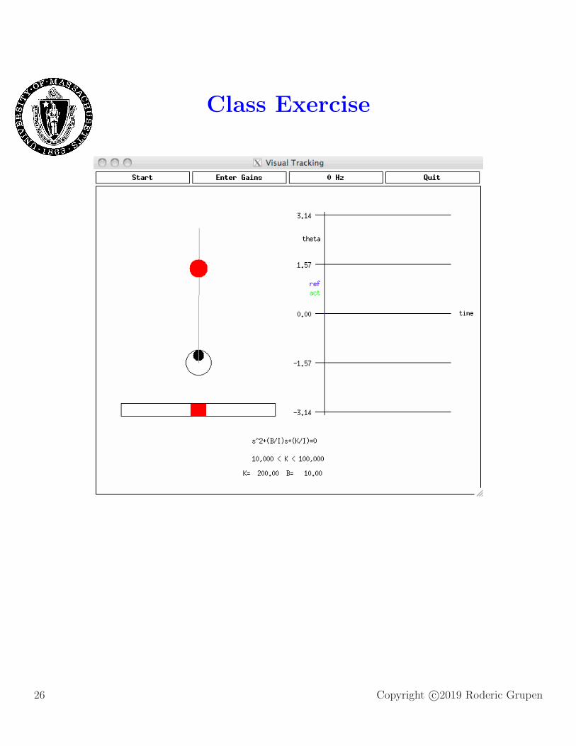
Class Exercise


Frequency-Domain Response

ζ = 0.1

0.2

0.4

1.0

2.0

(a)

|Ccltf(s)|s=iω

bandwidth:

power ratio = 1/2

response = 1/√2

ωωn

ζ = 0.1 0.2 0.41.02.0

(b)

|φcltf |s=iω

ωωn


Class Exercise


basic tools of linear control theorygrupen/403/slides/403control.pdf · •proposed the...

Documents