1

Basket optionsand implied correlations:a closed form approach

Svetlana BorovkovaFree University of Amsterdam

CFC conference, London, January 17-18, 2007

2

• Basket option: option whose underlying is a basket (i.e. a portfolio) of assets.

• Payoff of a European call basket option: is the basket value at the time of maturity ,

is the strike price.

( )+− XTB )()(TB T

X

3

Commodity baskets

• Crack spreads: Qu * Unleaded gasoline + Qh * Heating oil - Crude

• Soybean crush spread:Qm * Soybean meal + Qo * Soybean oil - Soybean

• Energy company portfolios:Q1 * E1 + Q2 * E2 + … + Qn En,

where Qi’s can be positive as well as negative.

4

Motivation:

• Commodity baskets consist of two or more assets with negative portfolio weights (crack or crush spreads), Asian-style.\

• The valuation and hedging of basket (and Asian) options is challenging because the sum of lognormal r.v.’s is not lognormal.

• Such baskets can have negative values, so lognormal distribution cannot be used, even in approximation.

• Most existing approaches can only deal with baskets with positive weights or spreads between two assets.

• Numerical and Monte Carlo methods are slow, do not provide closed formulae.

5

Our approach:

• Essentially a moment-matching method.• Basket distribution is approximated using a generalized family

of lognormal distributions : regular, shifted, negative regular or negative shifted.

The main attractions:• applicable to baskets with several assets and negative

weights, easily extended to Asian-style options • allows to apply Black-Scholes formula • provides closed form formulae for the option price and greeks

6

Regular lognormal, shifted lognormal and negative regular lognormal

7

Assumptions:

• Basket of futures on different (but related) commodities. The basket value at time of maturity T

where : the weight of asset (futures contract) i,: the number of assets in the portfolio,: :the futures price i at the time of maturity .

• The futures in the basket and the basket option mature on the same date.

( )∑=

=N

iii TFaTB

1

.)(

iaN

( )TFi

8

Individual assets’ dynamics:

Under the risk adjusted probability measure Q, the futures prices are martingales. The stochastic differential equations for is

where:the futures price i at time t:the volatility of asset i:the Brownian motions driving assets i and j with correlation

( )tFi

( )( ) ( ) NitdWtFtdF i

ii

i ,...,3,2,1,. )( ==σ

( )tFi

iσ( ) ( ) ( ) ( )tWtW ji ,

ji ,ρ

9

Examples of basket distribution:

9.0;1%;3;10];1;1[];3.0;2.0[];90;100[ ===−=−=== ρσ yearTrXaFo

9.0;1%;3;5];1;1[];2.0;3.0[];100;105[ ===−=−=== ρσ yearTrXaFo

Shifted lognormal

Negative shifted lognormal

10

The first three moments and the skewness of basket on maturity date T :

where : standard deviation of basket at the time T

( ) ( ) ( ) ( )∑∑∑= = =

++=N

kkjkjkikijijikj

N

j

N

iikji TTTFFFaaa

1...

1 1.........exp.0.0.0... σσρσσρσσρ

( ) ( )( )( )3

)(

3

)(TB

TBTBETBE

ση −

=

( )TBσ

( ) ( ) ( )∑=

==N

iii FaTMTBE

11 0.

( )( ) ( ) ( ) ( ) ( )∑∑= =

==N

j

N

ijijijiji TFFaaTMTBE

1 1,2

2 ...exp.0.0.. σσρ

( )( ) ( ) == TMTBE 33

11

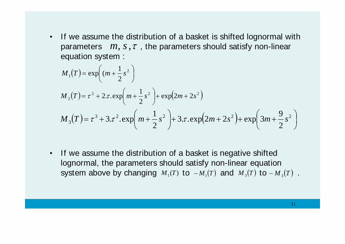
• If we assume the distribution of a basket is shifted lognormal with parameters , the parameters should satisfy non-linear equation system :

• If we assume the distribution of a basket is negative shifted lognormal, the parameters should satisfy non-linear equation system above by changing to and to .

τ,, sm

( ) ⎟⎠⎞

⎜⎝⎛ += 2

1 21(exp smTM

( ) ( )2222 22exp

21exp..2 smsmTM ++⎟

⎠⎞

⎜⎝⎛ ++= ττ

( ) ( ) ⎟⎠⎞

⎜⎝⎛ ++++⎟

⎠⎞

⎜⎝⎛ ++= 22223

3 293exp22exp..3

21exp..3 smsmsmTM τττ

)(1 TM ( )TM1− ( )TM 3 ( )TM 3−

12

Shifted lognormal

Regular lognormal

8.0;1%;3;150];1;1[

];3.0;2.0[];175;50[

====−=

==

ρ

σ

yearTrXa

Fo

13

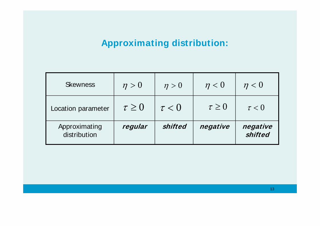
Approximating distribution:

negative shifted

negativeshiftedregularApproximating distribution

Location parameter

Skewness 0>η 0>η 0<η

0≥τ 0≥τ0<τ 0<τ

0<η

14

Valuation of a call option(shifted lognormal):

• Suppose that the distribution of basket 1 is lognormal. Then the option on such basket can be valued by applying theBlack-Scholes formula.

• Suppose that the relationship between basket 2 and basket 1 is

• The payoff of a call option on basket 2 with the strike price is:

It is the payoff of a call option on basket 1 with the strike price

( ) τ+= tBtB )1()2( )(

X

( )( ) ( )( )( ) ( ) ( )( )++−−=−+=− ττ XTBXTBXTB )1()1()2(

( )τ−X

15

Valuation of call option (negative lognormal):

• Suppose again that the distribution of basket 1 is lognormal. Then the option on such basket can be valued by applying theBlack-Scholes formula.

• Suppose that the relationship between basket 2 and basket 1 is

• The payoff of a call option on basket 2 with the strike price is:

It is the payoff of a put option on basket 1 with the strike price

( ) ( )tBtB )1()2( −=

X

( )( ) ( )( ) ( ) ( )( )++−−=−−=− TBXXTBXTB )1()1()2(

X−

16

Closed form formulae of a basket call option:

• For e.g. shifted lognormal :

where

It is the call option price with strike price .

( ) ( )( ) ( ) ( ) ( )[ ]211 ..exp dNXdNTMrTc ττ −−−−=

( )( ) ( )V

VXTMd

21

121loglog +−−−

=ττ

( )( ) ( )V

VXTMd

21

221loglog −−−−

=ττ

( ) ( )( )( ) ⎟

⎟⎠

⎞⎜⎜⎝

⎛

−+−

= 21

212 ..2logτ

ττTM

TMTMV

( )τ−X

17

Algorithm for pricing general basket option:

• Compute the first three moments of the terminal basket value andthe skewness of basket.

• If the basket skewness is positive, the approximating distribution is regular or shifted lognormal. If the basket skewness is negative, the approximating distribution is negative or negativeshifted lognormal.

• By moments matching of the appropriate distribution, estimate parameters .

• Choose the approximating distribution on the basis of skewness and the shift parameter .

τ,, sm

τ

ηη

18

Simulation results:

%3;1;8.0;9.0;30];5.0;8.0;1[

];25.0;3.0;2.0[];105;90;95[:5

3,13,22,1

==

===−=−−=

==

ryearT

XaFoBasket

ρρρ

σ

0; <τ0<η

Call price: 7.7587

(7.7299)

(neg. shifted)

19

%3;1;8.0;9.0

;35];1;8.0;6.0[];2.0;3.0;25.0[];95;90;100[

:6

3,13,22,1

==

====−===

ryearT

XaFoBasket

ρρρ

σ

0>η 0; <τ (shifted)

Call price : 9.0264

(9.0222)

20

Location parameter

skewness

35-30-140104-5020Strike price

(X)

0.90.8

0.90.8

0.80.80.30.9Correlation

[0.6;0.8; -1][1; -0.8; -0.5][-1;1][0.7;0.3][-1;1][-1;1]Weights

(a)

[0.25;0.3;0.2][0.2;0.3;0.25][0.1;0.15][0.2;0.3][0.3;0.2][0.2;0.3]Volatility

[100;90;95][95;90;105][200;50][50;175][150;100][100;120]Futures price

(Fo)

Basket 6Basket 5Basket 4Basket 3Basket 2Basket 1

0>η

0<τ

)(η

)(τ

)(σ

)(ρ== 3,22,1 ρρ

=3,1ρ

0<η

0>τ

== 3,22,1 ρρ=3,1ρ

0>η 0>η0<η0<η

0>τ0<τ 0<τ 0<τ

T=1 year; r = 3 %

21

Monte carlo

Kirk

Bachelier

Our approach

Method

7.7299(0.0095)

-

-

7.7587neg.

shifted

Basket 5

9.0222(0.0151)

1.9663(0.0044)

10.8211(0.0183)

16.7569(0.0224)

7.7441(0.0143)

-1.5065-16.67777.7341

-2.1214-17.23658.0523

9.0264shifted

1.9576neg.

regular

10.8439 regular

16.9099neg.

shifted

7.7514

shifted

Basket 6Basket 4Basket3Basket 2Basket 1

22

Performance of Delta-hedging:

• Hedge error: the difference between the option price and the discounted hedge cost (the cost of maintaining the deta-hedged portfolio); computed on the basis of simulations.

• Plot the ratio between the hedge error standard deviation to call price vs. hedge interval.

• Mean of hedge error is 4 % for basket 1 and 7 % for basket 2.

%3;1;10;9.0];1;1[];15.0;1.0[];110;100[:1====−=

==ryearTXa

FoBasketρ

σ

%3;1;30;8.0;9.0];5.0;8.0;1[]25.0;3.0;2.0[];105;90;95[:2

3,13,22,1

==−=

===−−===

ryearTXa

FoBasketρρρ

σ

23

Greeks: correlation vegaSpread [110,10], vols=[0.15,0.1]

−1

−0.5

0

0.5

1

−10

0

10

20

30

40−10

−8

−6

−4

−2

0

correlationstrike price

vega

with

resp

ect to

corre

lation

24

Correlation vegavs. correlation and vs. strike

−1 −0.8 −0.6 −0.4 −0.2 0 0.2 0.4 0.6 0.8 1−10

−8

−6

−4

−2

0

2

correlation

vega

with

res

pect

to c

orre

latio

n

−10 −5 0 5 10 15 20 25 30 35 40−10

−9

−8

−7

−6

−5

−4

−3

−2

−1

0

strike priceve

ga w

ith r

espe

ct to

cor

rela

tion

25

Volatility vegas vs. volatilitiessame spread, X=10, correlation=0.8

0.050.1

0.150.2

0.250.3

0.350.4

0

0.1

0.2

0.3

0.4−40

−30

−20

−10

0

10

20

30

40

50

sigma 1sigma 2

vega w

ith r

esp

ect

to s

igm

a 1

0.050.1

0.150.2

0.250.3

0.350.4

0

0.1

0.2

0.3

0.4−40

−30

−20

−10

0

10

20

30

40

sigma 2sigma 1

vega w

ith r

esp

ect

to s

igm

a 2

26

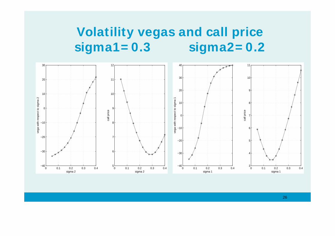
Volatility vegas and call pricesigma1=0.3 sigma2=0.2

0 0.1 0.2 0.3 0.4−40

−30

−20

−10

0

10

20

30

sigma 2

veg

a w

ith r

esp

ect

to

sig

ma

2

0 0.1 0.2 0.3 0.45

6

7

8

9

10

11

12

sigma 2

call

price

0 0.1 0.2 0.3 0.4−40

−30

−20

−10

0

10

20

30

40

sigma 1ve

ga

with

re

spe

ct t

o s

igm

a 1

0 0.1 0.2 0.3 0.43

4

5

6

7

8

9

10

11

sigma 1

call

price

27

Asian baskets

•Underlying value: (arithmetic) discrete average basket value over a certain interval•The same approach as above applies, because

So the average basket value is simply the basket of individual assets’ averages, with the same weights, so

the above approach applies directly, only with different moments! option prices and greeks again calculated analytically.

∑∑ ∑∑ == =====

N

i iit

tk

N

i kiit

tk kB TAatFan

tBn

TA nn

11)()(1)(1)(

11

28

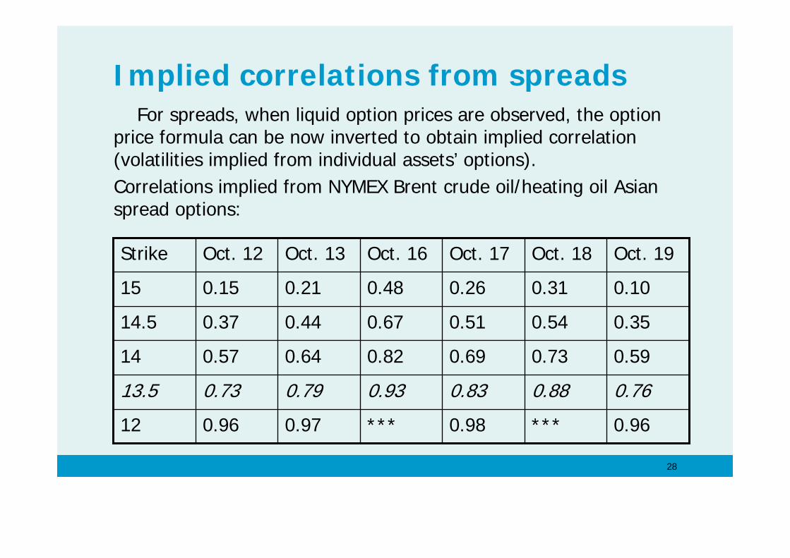
Implied correlations from spreadsFor spreads, when liquid option prices are observed, the option

price formula can be now inverted to obtain implied correlation (volatilities implied from individual assets’ options).Correlations implied from NYMEX Brent crude oil/heating oil Asian spread options:

0.96***0.98***0.970.9612

0.760.880.830.930.790.7313.5

0.590.730.690.820.640.5714

0.350.540.510.670.440.3714.5

0.100.310.260.480.210.1515

Oct. 19Oct. 18Oct. 17Oct. 16Oct. 13Oct. 12Strike

29

Implied correlations vs strikes

12 12.5 13 13.5 14 14.5 150

0.2

0.4

0.6

0.8

1

1.2

1.4

strike price ($/bbl)

impli

ed co

rrelat

ion

30

Conclusions

Our proposed method:Has advantages of lognormal approximationApplicable to several assets, negative weights and Asian basket optionsProvides good approximation of option pricesGives closed-form expressions for the greeksPerforms well on the basis of delta-hedgingAllows to imply correlations from liquid spread options