bayesian estimation of non-stationary markov models...

Bayesian Estimation of Non-Stationary Markov Models Combining

Micro and Macro Data

Hugo Storm

1, Thomas Heckelei

2, Ron C. Mittelhammer

3

1 Institute for Food and Resource Economics, University of Bonn, Germany,

[email protected] 2 Institute for Food and Resource Economics, University of Bonn, Germany,

[email protected] 3 School of Economic Sciences, Washington State University, Pullman, USA,

[email protected]

The paper was part of the organized session “Understanding changes in the farm size distribution, entry

and exit”

at the EAAE 2014 Congress ‘Agri-Food and Rural Innovations for Healthier Societies’

August 26 to 29, 2014

Ljubljana, Slovenia

Copyright 2014 by Hugo Storm, Thomas Heckelei and Ron C. Mittelhammer. All rights

reserved. Readers may make verbatim copies of this document for non-commercial purposes

by any means, provided that this copyright notice appears on all such copies.

1

Bayesian Estimation of Non-Stationary Markov Models Combining

Micro and Macro Data

Hugo Storm, Thomas Heckelei, Ron C. Mittelhammer

Abstract: We develop a Bayesian framework for estimating non-stationary Markov

models in situations where macro population data is available only on the

proportion of individuals residing in each state, but micro-level sample data is

available on observed transitions between states. Posterior distributions on non-

stationary transition probabilities are derived from a micro-based prior and a

macro-based likelihood using potentially asynchronous data observations,

providing a new method for inferring transition probabilities that merges previously

disparate approaches. Monte Carlo simulations demonstrate how observed micro

transitions can improve the precision of posterior information. We provide an

empirical application in the context of farm structural change.

Keywords: data combination; Markov process; micro and macro data; transition

probabilities

JEL classification codes: C11, C81

1. Introduction

A new Bayesian framework for inferring the transition probabilities of non-stationary

Markov models is developed in this paper. Non-stationary Markov models facilitate analysis

of factors influencing the probability that an individual will transition between predefined

states. Data used for estimating Markov models can either be panel data, where the specific

movement of an individual between states is observed over time, or aggregated data,

providing only the number of individuals residing in each state over time. Following Markov

terminology, we refer to such panel data and aggregated data as micro and macro data,

respectively. The overall objective of our approach is to combine micro and macro

information into a unified and consistent methodology for estimating transition probabilities.

In recent years Markov models have been popular in the context of farm structural

change analysis (Karantininis 2002, Huettel and Jongeneel 2011, Zimmermann and Heckelei

2012a, Zimmermann and Heckelei 2012b, Arfa et al. 2014). For estimation, they rely on the

generalized cross-entropy (GCE) approach, proposed by Golan and Vogel (2000) and first

applied in a Markov context by Karantininis (2002). The GCE approach allows including

prior information in the estimation. In the Markov context, prior information is typically

specified for the transition probabilities and can be based on previous studies, theory or expert

knowledge. Considering prior information allows estimating ill-defined systems which is the

major strength of the GCE approach. On the other hand the use of prior information is often

2

criticized for introducing subjective prior beliefs. This criticism is addressed by Zimmermann

and Heckelei (2012a) using macro data from the farm structural survey (FSS; Council

Regulation (EC) No 1166/2008) in combination with micro data from the Farm accountancy

network (FADN; Council Regulation (EC) No 1217/2009). The micro data is used to specify

prior information on the transition probabilities in the GCE approach avoiding an otherwise

rather ad hoc prior specification. Despite these contribution general shortcomings of the GCE

approach persists. Particularly, the rather non-transparent way prior information is specified

and used in estimation makes it difficult for the researcher and the research community to

assess its influence. Further, it is not possible to specify an ignorance (or non-informative)

prior for cases where no prior information is available (Heckelei et al., 2008). An additional

shortcoming of the approach proposed by Zimmermann and Heckelei (2012a) is that it

ignores the precision of prior information in the micro data. Thus micro and macro data is not

weighted in estimation and the final results are independent of the size of the micro sample.

Further, the approach requires the specification of reference distributions for residuals,

including the specification of support points, which determine the signal-to-noise ratios in the

Markov transition equations a priori. Lastly, since FSS data is only available every two to

three years, the approach requires interpolating FSS macro data on a yearly basis.

Apart from the analysis of farm structural change the idea of combining micro and

macro data was considered previously in the context of a medical application by Hawkins and

Han (2000). They analyzed macro data obtained in repeated independent cross sectional

surveys within a city district together with limited micro data obtained from respondents who

were ‘coincidently’ interviewed in two consecutive cross sectional surveys. The behaviour

under study was the benefits of an intervention program attempting to modify drug use-

related behaviour, and their Markov model was a two-state process relating to awareness, or

not, of the health consequences of not bleaching shared drug needles. They defined a linear

model, within the Classical statistical framework, that explained the binary marginal

probabilities of being in one of the two awareness states in a certain time period (based on

‘standard observed proportion estimates’ from aggregate data) as well as transition

probabilities relating to transitions between the two states (from the micro data).

Generalizations of Hawkins and Han’s binary state model to multinomial transitions are

conceptually possible, but the parameter dimensionality, as well as the complexity of the

covariance structure and constraint set imposed by the sampling design, quickly renders their

general linear model approach intractable as the number of states increase beyond two.

In contrast to the previous two Classical approaches, our Bayesian framework provides a

flexible and tractable method of combining micro and macro data generating processes that is

logically consistent and coherent within the tenets of the probability calculus while

accommodating a relatively large number of Markov states. The rather complicated linkages

between transition probabilities and observed Markov state outcomes, and the complex

parametric constraints and covariance matrix structure of the combination of micro and macro

data generating processes, are specified consistently as a matter of course in specifying the

posterior probability distribution for the parameters of the transition equation. Moreover, the

Bayesian framework allows prior information to be incorporated into the estimation of non-

stationary Markov models within an established coherent probabilistic framework. In

addition, the Bayesian methodology provides a natural and relatively straightforward way of

3

combining data observations at either the macro or micro level that are asynchronous1, which

is in contrast to the methods offered heretofore. Also we devise different specifications for

both ordered and unordered Markov states, which is yet another flexible feature of the

method. Overall, the Bayesian approach that we present offers a tractable full posterior

information approach for combining micro and macro data-based information on non-

stationary transition probabilities that allows the estimation of functional relationships linking

transition probabilities with their determinants.2

Even though our focus is on combining micro and macro data it should be pointed out

that the approach is also relevant for cases when no micro data is available. In these cases the

approach allows specifying an ignorance prior such that a consistent estimation of non-

stationary Markov model with only macro data is possible. This is an important feature

compared to the GCE approach in which each specification (even a uniform distribution)

implies some form of prior information (Heckelei et al., 2008).

Despite the analysis of farm structural change which is the primary focus here the

proposed approach is equally relevant for other applications for which both macro and micro

data is available. One example is an analysis of voter transitions in political science. Here,

macro data on the vote shares of candidates is available from official statistics, whereas micro

data can be obtained from voter (transition) surveys (McCarthy and Tyan 1977, Upton 1978).

Additional examples of similar data situations can be found in the context of Ecological

inference problems, which are closely related to Markov processes (Wakefield 2004,

Lancaster et al. 2006). In general the proposed approach is relevant for all situations in which

the micro sample is relatively small compared to the macro data. If the micro sample is

relatively large the macro sample does not contribute additional information such that an

approach relaying exclusively on the micro data is sufficient.

The paper is organized as follows: First, the Bayesian framework for non-stationary

Markov models is developed in section 2. Two different specifications of the transition

probabilities, that of ordered and unordered Markov states, are discussed, appropriate

likelihood functions and prior densities are defined, and issues relating to computational

implementation are identified. Then the design and results of a Monte Carlo simulation

experiment are presented in section 3 and used to assess how the inclusion of prior

information affects the posterior as well as the numerical stability of the sampling algorithm,

and the degree to which estimator performance is improved under different micro sample

sizes for both specifications. In section 4 the methodological framework is applied

empirically in the context of an analysis of farm structural change in Germany. The

application demonstrates how the framework can facilitate estimation in a situation where

estimation with either micro or macro data alone would suffer from several limitations.

Section 5 provides conclusions and a discussion of areas for further research.

1 By “synchronous” we mean both that observations over time occur in sequence without gaps (follow a tact) and that the

micro and macro data are observed for the same time units. 2 In their pedagogical contribution to the use of MCMC computational methodology Pelzer and Eisinga (2002) include an

example of a Bayesian approach specifically designed for a two state Markov model which depends crucially on the

characteristics of a Bernoulli process. The specification of prior information in their example is effectively ad-hoc, whereas

our specification is fully consistent with the structure of the data generating process. Moreover, their example does not

generalize to either stationary or non-stationary multinomial Markov processes.

4

2. Bayesian Approach for Non-Stationary Markov Models

Markov processes provide a conceptual model for the movement of individuals between a

finite number of predefined states, 1,...,i k , within the context of a stochastic process. The

k states are mutually exclusive and exhaustive. A Markov process is characterized by a

k k transition probability (TP) matrix3 tP . The elements ijtP

of tP represent the probability

that an individual moves from state i in time 1t to j in time t . The 1k -vector tn

denotes the number of individuals in each state i at time t and evolves over time according to

a (first order) Markov process

1t t tn P n . (1)

In a non-stationary Markov process, the TPs change over time periods4 0,1,...,t T .

Data used for estimating a non-stationary Markov process can either be macro or micro level.

In the case of macro data, only the aggregate numbers of individuals in the states, ,tn is

observed at each time period. For micro data, the movement of each individual between states

is also observed over time. Thus, the k k -matrix tN with elements ijtn representing the

number of individuals that transition from state i at 1t to j in t , is directly observed.

In this section we assume data observations are synchronous, as defined in footnote 1,

both for ease of exposition and to be consistent with precedence in the literature. However,

the proposed approach is considerably more flexible in that asynchronous data can be

analyzed in a straightforward way, and in the empirical application in section 4, macro data

available only every two to three years will be combined with yearly micro data. Similarly,

the reverse case, where macro data has a higher temporal resolution than the micro data, can

be considered as well.

The structural specification of the TP matrix tP depends on the underlying behavioural

model. In the following subsection we review TP matrix specifications corresponding to

ordered as well as unordered Markov states to define notation and establish the foundation for

the definition of the posterior. Then the data likelihood function, representing the macro data,

and a prior density, representing the micro data are defined and combined into the posterior

distribution for the TPs.5 The last subsection presents computational methodology relating to

the use of the posterior distribution for inference purposes.

Specification of the Transition Probability Matrix

For appropriate specification of the TPs, the nature of the relationship between Markov

states need to be considered, and we discuss two different behavioural models that

differentiate between ordered and unordered Markov states. We argue that for ordered

3Bold letters are used for vectors or matrices. 4Depending on the problem context, one could also consider only two time periods observed over various regions, or a

combination of multiple time and regional observations. 5 In his dissertation, Rosenqvist (1986) introduces the conceptual rudiments of combining micro and macro data in a prior-

likelihood framework. However, the analysis was restricted to stationary processes with synchronous observations and the

micro and macro data observations were assumed to be disjoint. Our Bayesian framework is not constraint by any of these

assumptions and moreover, we provide a tractable empirical method of implementation.

5

Markov states the ordered logit model is superior to the more common multinomial logit

model with respect to both model assumptions and from a computational point of view.

In cases where the states of the Markov process are unordered, the multinomial logit

model is a suitable specification for the TPs6. The specification based on the multinomial logit

model assumes that the transition of individuals between different states can be represented

by a random utility model. The utility that would accrue to individual l upon moving from

state i in 1t to j in t is denoted as ,ijtl ijt ijtlU V where the deterministic component of

utility is specified as 1ijt t ijV z b , with 1tz being a vector of lagged exogenous variables. The

deterministic part varies only over time and not over individuals because aggregated (macro)

data is considered. Consequently, the deterministic component of utility reflects exogenous

variables that affect the utility of all individuals alike. The random error ijtl varies over time

and individuals. It is assumed that an individual chooses a transition that maximizes her utility

ijtlU . The assumption that ijtl are iid random draws from a Gumbel distribution result in a

multinomial logit specification for each row of tP .

If the Markov states are ordered, an ordered choice model is an appropriate specification

for the underlying behavioral model. In this case it is assumed that there exists an unobserved

continuous latent variable *

itlY for each individual l that determines the outcome of the

observed variable itlY according to

*

1if , 1,...,itl j itl jY j c Y c i j k (2)

where the jc ’s are the thresholds for each Markov state, with o kc and c . The

index i indicates that an individual was in state i at 1t . The unobserved latent variable *

itlY

consists of a deterministic part 1t iz β plus a random part *

itl . The vector of unknown

parameters iβ are allowed to differ between the k different states in 1t . As in the

preceding multinomial logit model, the deterministic part varies over time but not over

individuals. Assuming that *

it are iid random draws from a logistic distribution7 results in an

ordered logit model for each row of tP .

One important difference between the ordered logit and the multinomial logit model is

that only one error term, instead of one error term for each alternative, is considered for each

individual. This implies that the assumption of ‘Independence of Irrelevant Alternatives’ (IIA)

does not apply to the ordered logit model. This is more appropriate whenever the alternatives

are ordered since in this case it can be expected that the error associated with one state is more

similar to the error of an alternative close to it than to an alternative further away (Train

2009). Also from a computational point of view, the ordered logit specification is often

6 A multinomial probit model could be an appropriate alternative for the error structure specification, but is left for future

work. 7 Assuming that the

*

it are random draws from a normal distribution would result in a probit (see footnote 6).

6

preferable since only 2zk n k k parameters8 need to be estimated, as compared to

( 1) zk k n parameters for the multinomial logit model.

A further advantage of the ordered choice model is that the interpretation of the latent

variable is often straightforward. For example, in the case of farm structural change noted in

the introduction, where Markov states refer to firm size classes, the latent variable can be

interpreted directly as firm size (see section 4). In the medical context where classes refer to

different stages of illness, the latent variable can be interpreted as the degree of illness.

However, the decision between an ordered and unordered choice model is not always

straightforward and can depend on the problem context as well as decision makers’

behavioural characteristics. In the voter transition example, one could regard the candidates as

unordered choices, but alternatively one could also argue that they are ordered according to a

one-dimensional political spectrum (‘right’ to ‘left’), in which case both models have

justification and the choice between the two must be guided by additional theoretical and/or

substantive behavioural arguments.

Posterior

The posterior is defined as the joint density of a micro data prior and a macro data

likelihood. Since micro and macro data are interdependent, the likelihood is the conditional

density of the macro data given the micro data. The prior density represents information

derived from a sample of micro observations on state transitions. It should be pointed out that

the distinction between prior and likelihood is somehow artificial. Both are likelihood

specification representing two different data sets. Also they are sampled at the same time

which usually distinguishes prior and likelihood information. The labeling is thus more a

convention and is motivated from the works in the context of the entropy estimation by

Zimmermann and Heckelei (2012a), mentioned above, using micro data to specify the support

and prior densities in an entropy estimation based on macro data.

The foundation for the likelihood function is provided by the first-order non-stationary

Markov process proposed by MacRae (1977). For the specification of a macro data based

likelihood function MacRae (1977) points out that the nature of the likelihood specification

depends critically on whether the state proportions, tx , are observed over time for the entire

population of size N , which she refers to as perfect observations, or whether the state

proportions, ty , are only a random sample of size tM N drawn and observed at each time

period, referred to as imperfect observations. In the case of perfect observations the

distribution of tx is fully characterized by 1tx . However, for imperfect observations the

distribution of ty also depends on earlier observations, 2 0,...,ty y , which provide additional

information on .ty For the latter case MacRae (1977) proposed a limited information

likelihood approach which is appropriate whenever macro data is available for only a sample

of the population. In the following, we focus on the case of perfect observations, i.e., a census

type of macro data set, which characterizes the type of data available in our empirical

application provided in section 4.

8 If a constant is included and 1c is normalized to zero 2k k cut points need to be estimated in addition to one

parameter for each explanatory variable and state (z

k n ) .

7

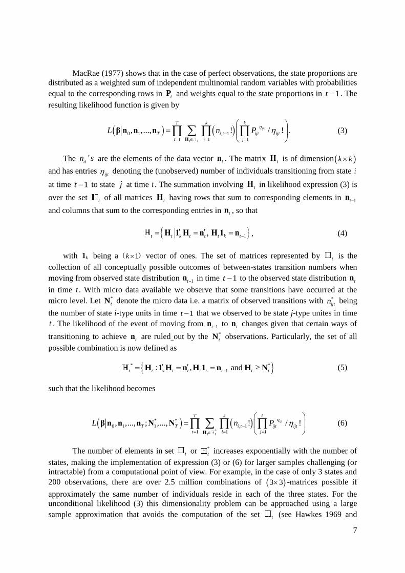
MacRae (1977) shows that in the case of perfect observations, the state proportions are

distributed as a weighted sum of independent multinomial random variables with probabilities

equal to the corresponding rows in tP and weights equal to the state proportions in 1t . The

resulting likelihood function is given by

0 1 , 1

1 1 1

, ,..., ! / !ijt

t t

T k k

T i t ijt ijt

t i j

L n P

Η

β n n n . (3)

The 'itn s are the elements of the data vector tn . The matrix tΗ is of dimension k k

and has entries ijt

denoting the (unobserved) number of individuals transitioning from state i

at time 1t to state j at time t . The summation involving tΗ in likelihood expression (3) is

over the set t of all matrices tΗ having rows that sum to corresponding elements in 1tn

and columns that sum to the corresponding entries in tn , so that

1,t t k t t t k t Η 1 Η n Η 1 n ,

(4)

with k1 being a 1k vector of ones. The set of matrices represented by t is the

collection of all conceptually possible outcomes of between-states transition numbers when

moving from observed state distribution 1tn in time 1t to the observed state distribution tn

in time t . With micro data available we observe that some transitions have occurred at the

micro level. Let *

tN denote the micro data i.e. a matrix of observed transitions with *

ijtn being

the number of state i-type units in time 1t that we observed to be state j-type unites in time

t . The likelihood of the event of moving from 1tn to tn changes given that certain ways of

transitioning to achieve tn are ruled out by the *

tN observations. Particularly, the set of all

possible combination is now defined as

* *

1: , and t t s t t t s t t t H 1 H n H 1 n H N (5)

such that the likelihood becomes

*

* *

0 1 1 , 1

1 1 1

, ,..., ; ,..., ! / !ijt

t t

T k k

T T i t ijt ijt

t i j

L n P

Η

β n n n N N (6)

The number of elements in set t or *

t increases exponentially with the number of

states, making the implementation of expression (3) or (6) for larger samples challenging (or

intractable) from a computational point of view. For example, in the case of only 3 states and

200 observations, there are over 2.5 million combinations of 3 3 -matrices possible if

approximately the same number of individuals reside in each of the three states. For the

unconditional likelihood (3) this dimensionality problem can be approached using a large

sample approximation that avoids the computation of the set t (see Hawkes 1969 and

8

Brown and Payne 1986). The large sample approximation used the property that the

multinomial distribution can be approximated with a multivariate normal distribution in large

samples. In our case each i -th row itH of tH is multinomial with size , 1i tn over 1,...,k

categories. If , 1i tn is large itH is approximately multivariate normal with mean *, 1i it i tn μ P ,

where *itP denotes the i row of tP without the element of the last column, and covariance

matrix * * *, 1i i t it it itn diag V P P P , where diag denotes a square matrix with the argument

vector as the main diagonal and zero off-diagonal elements. Since transitions between

observations are independent, each row of tH is independent and the probability of tH is

approximately equal to a multivariate normal random 1 1k k vector * *1 ....t t ktM H H with

mean 1[ ... ]k μ μ μ and variance

1

2

0 0

0 0

0 0 k

V

VV

V

. (7)

Defining * *1 ... kB I I , with *

iI being an identity matrix of size 1k , we have t tBM n .

Using that each linear transformation of a multivariate normal random variable is also

multivariate normal it follows that tn is multivariate normal with mean * *1t tBμ P n and

variance

* * * * *1 1t t t t tdiag BVB P n P n P Γ , (7)

where *tP and *

tn is equal to tP and tn without the last column and row, respectively.

Therefore, the probability of tn given 1tn can be approximated by a normal density such that

*

1 1; ,t t t t tP n n n P n Γ . From this it follows that (3) can be approximated by a large

sample log-likelihood, laL , given by

0 1

1* * * *

1 1

1

, ,...,

0.5 log .

a T

T

t t t t t t t t

t

L

β n n n

Γ n P n Γ n P n

(8)

When considering the micro observations, itH is still multinomial with size , 1i tn over

1,...,k categories except that the constraint *it itH N need to be considered. As argued above

the approach is intended for situation in which the micro data is only available for a fraction

of the observation in the macro data. In these situations the limits imposed by *it itH N are

hardly binding such that the approximation of tH by a multivariate normal remains valid. The

validity of this large sample approximation is assessed in the Monte Carlo simulations

considering different sizes of the micro sample.

9

The specification of the prior density p β , considers the underlying sampling

distribution of the micro observations. Recall that itn is the number of individuals that were in

state i at time t , let i

tX be the vector of shares across states in t for individuals who were in

state i in 1t , and let itP be the i -th row of tP . The propensity of each individual in the

micro sample to transit between states is in accordance with the appropriate elements of tP .

Analogous to the case of macro data, the distribution across states in t of individuals who

were in state i in 1t is multinomial around mean itP with size itn . The observed number of

individuals in each of the k states in t, , 1,...,itn i k , is then the corresponding weighted sum

of vectors , 1,..., .i

t i kX Therefore, the prior density can be represented as a likelihood

similar to (3), except that now information about the individual transitions ijtn is available,

making the summation over the set t unnecessary because the actual transitions are

observed. Hence the likelihood simplifies to

1 , 1

1 1 1

,..., ! / !ijt

T k kn

T i t ijt ijt

t i j

p L n n

β β N N P , (9)

where the k k -matrix tN has elements ijtn representing the number of individuals

that transition from state i at 1t to j in t . We emphasize that for the case of aggregated

data discussed above, the distribution of tn differs between imperfect and perfect

observations, while for micro observations, this distinction does not apply. In the latter case,

the distribution of tx is fully characterized by 1tx regardless of whether a sample or the entire

population is observed. The fundamental difference is that in the case of micro observations,

individuals in the sample in time period t are all the same as in 1t which is usually not the

case for macro data. Consequently, information earlier than 1tx

contains no additional

information about tx .

Computational Implementation

In order to conduct inference in the model depicted above, integrating and/or taking

expectations based on the posterior density h β d * *

0 1 1, ,..., ; ,...,T TL pβ n n n N N β or on

its approximation 0 1, ,...,a a Th L pβ d β n n n β is required. An analytical approach to

such computations is generally intractable. Instead a Monte Carlo integration approach is

implemented based on sampling from the posterior density via a Metropolis Hastings (MH)

algorithm.9 For our purposes, we evaluate the optimal Bayesian estimator under quadratic

9 An interesting alterative to the simple random walk MH sample would be the development of a data augmentation sample

algorithm, in the spirit of Albert and Chib (1993), for a non-stationary Markov model using aggregated data. Our first

implementation of such an algorithm, building on Musalem et al. (2009) who proposed a concept to consider aggregated data

in an simple ordered logit model, suffered, however, form slow convergence problems. Convergence problems are known for

the Albert and Chib (1993) algorithm and could be overcome using alternatives such as those proposed by Frühwirth-

Schnatter and Frühwirth (2007) or Scott (2011). These algorithms, however, focus on simple multinomial logit models and

are not directly transferable to the Markov case using aggregated data.

10

loss, the posterior mean, by calculating the mean of an iid sample from h β d for sufficiently

large sample sizes.

Specifically, a random walk MH algorithm with a multivariate normal generating

density is employed.10

The variance of the proposal density is adjusted such that an

acceptance rate in the interval .2, .3 is obtained. In cases where the number of parameters to

be estimated is large, a ‘Block-at-a-Time’ algorithm proposed by Chib and Greenberg (1995)

is employed in which the parameters to be estimated are divided into blocks.

3. Monte Carlo Simulation of Prior Information Effects

In this section we analyze the influence of prior information, in the form of a sample of

micro observations, on the posterior distribution and associated estimators’ performance as

well as on the behaviour of the sampling algorithm. Based on an underlying population of

10,000indn individuals, four different scenarios are considered regarding the availability of

prior information, including a case of no micro observations, and micro samples of n = 100,

500, and 1000. The scenarios are further distinguished by the number of Markov states (

3,4,5k ). Data is generated for 100T time periods and 6zn explanatory variables

including a constant. All simulations are undertaken for a Markov model based on either the

multinomial logit specification or the ordered logit specification discussed above, and are

performed using Aptech’s GAUSSTM

11.

Data Generating Process

The data generating process distinguishes between the two different behavioural models,

based on the multinomial logit and ordered logit specification discussed in section 2. In both

cases the parameterization is chosen so that the deterministic part constitutes roughly one

third of the model’s total variation. Furthermore, in both cases indn individuals are considered

that transition over time between the k states in accordance with the underlying behavioural

model. The initial state of each individual in 1t is randomly chosen with probability equal

to 1,...,iu i k , where the probability is the same for all individuals and given by

1

k

i i h

h

u u u

with ~ 0,1iu iid , where ,a b denotes the continuous uniform

distribution on the interval a to b.

In the multinomial logit model each individual l chooses the state of the next period

based on the utility, ijtlU , associated with a specific transition from state i in 1t to j in t .

The utility ijtl ijt ijtlU V

consists of a deterministic part 1ijt t ijV z b and an individual

random part ijtl and is generated by drawing the elements of the (lagged) exogenous

variables 1tz from 1,4 and the elements of the 1zn ‘true’ parameter vectors ijb

from 1,1 . Since only differences in utilities are relevant, the parameters of the last

10 To mitigate computer overflow problems the Metropolis acceptance ration is calculated as

, min exp ln ln ,1rcan c nr ah h

β β β d β d .

11

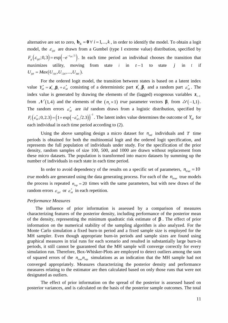
alternative are set to zero, 1,...,ik i k b 0 , in order to identify the model. To obtain a logit

model, the ijtl are drawn from a Gumbel (type I extreme value) distribution, specified by

3;0,3 exp ijtl

g ijtlF e

. In each time period an individual chooses the transition that

maximizes utility, moving from state i in 1t to state j in t if

1 2, ,..., .ijtl i tl i tl iktlU Max U U U

For the ordered logit model, the transition between states is based on a latent index

value * *

1itl t i itlY z β consisting of a deterministic part 1t i

z β and a random part *

itl . The

index value is generated by drawing the elements of the (lagged) exogenous variables 1tz

from 1,4 and the elements of the 1zn true parameter vectors iβ from 1,1 .

The random errors *

itl are iid random draws from a logistic distribution, specified by

1

* *;0,2.3 1 exp 2.3l itl itlF

. The latent index value determines the outcome of itlY for

each individual in each time period according to (2).

Using the above sampling design a micro dataset for indn individuals and T time

periods is obtained for both the multinomial logit and the ordered logit specification, and

represents the full population of individuals under study. For the specification of the prior

density, random samples of size 100, 500, and 1000 are drawn without replacement from

these micro datasets. The population is transformed into macro datasets by summing up the

number of individuals in each state in each time period.

In order to avoid dependency of the results on a specific set of parameters, 10truen

true models are generated using the data generating process. For each of the truen true models

the process is repeated 20repn times with the same parameters, but with new draws of the

random errors ijtl or *

itl in each repetition.

Performance Measures

The influence of prior information is assessed by a comparison of measures

characterizing features of the posterior density, including performance of the posterior mean

of the density, representing the minimum quadratic risk estimate of . The effect of prior

information on the numerical stability of the sampling algorithm is also analyzed. For the

Monte Carlo simulation a fixed burn-in period and a fixed sample size is employed for the

MH sampler. Even though appropriate burn-in periods and sample sizes are found using

graphical measures in trial runs for each scenario and resulted in substantially large burn-in

periods, it still cannot be guaranteed that the MH sample will converge correctly for every

simulation run. Therefore, Box-Whisker-Plots are employed to detect outliers among the sum

of squared errors of the true repn n simulations as an indication that the MH sample had not

converged appropriately. Measures characterizing the posterior density and performance

measures relating to the estimator are then calculated based on only those runs that were not

designated as outliers.

The effect of prior information on the spread of the posterior is assessed based on

posterior variances, and is calculated on the basis of the posterior sample outcomes. The total

12

variance of the posterior density is calculated by summing over the posterior variances of all

zn parameters for each run, and then the mean over all true repn n simulation runs (outliers

excluded) is calculated to obtain one scalar value measure of the total variance.

The analysis of the influence of prior information on the Bayes estimator (posterior

mean) is based on the mean square error (MSE) criterion, calculated as the mean sum of

squared errors between estimated and true parameter values, where the mean is calculated

over all of the true repn n simulation runs not detected as outliers. The MSE is further

decomposed into variance and bias components, where the squared bias is again summed over

all parameters. The distribution of the sum of squared errors together with the number of

outliers detected for each scenario provides an assessment of the numerical stability of the

MH sampler, and the effects of prior information on that numerical stability.

Results of the Monte Carlo Simulation

The results of the Monte Carlo Simulations for the multinomial logit model are presented

in Fig. 1. Results show that incorporating prior information in the form of a micro sample

decreases the total variance of the posterior density, and more so the larger the micro sample.

The variance reduction effect of prior information becomes even more pronounced the greater

the number of Markov states being considered. Similarly, prior information decreases the

MSE of the estimator, and a greater number of Markov states accentuate this effect.

Decomposing the MSE into bias and variance suggests that the MSE is primarily determined

by the variance of the estimator. In all scenarios the share of the squared bias is only 4 to 9 %

of total MSE.

The distribution of the sum of squared errors, as depicted in the Box-Whisker-Plots in

Fig. 1, provides information about the numerical performance of the MH sampling algorithm.

Results show that more simulation runs are detected as outliers in the no prior information

scenario (i.e. micro sample with 0 obs.), especially when considering 4k or 5k Markov

states. This observation indicates problems relating to the numerical stability of the MH

sampler, in the sense that the algorithm does not converge correctly for some simulation runs.

When considering a micro sample as prior information, substantially fewer simulation runs

are detected as outliers, indicating that the use of prior information improves the numerical

stability of MH sampler.

Comparable results are obtained for the ordered logit model as depicted in Fig. 2.

Similar to the multinomial logit simulation, results indicate that prior information reduces the

variance of the posterior density, and more so the larger the micro sample considered. The

same can be observed for the MSE, which decreases with increasing micro sample size. If

prior information is considered the MSE is mainly determined by the variance of the estimator

such that the share of the squared bias is only 4 to 6 % of total MSE in all scenarios. For the

no prior information scenarios, however, the bias share is substantially larger, being between

23 and 28 %.

13

Number of Markov states: k=3

Size of micro sample

Measures 0

10

0

50

0

10

00

Variancea,

Posterior

0.

00592

0.

00496

0.

00312

0.

00219

MSEa,

Estimator

0.

00892

0.

00672

0.

00414

0.

00275

Sq. Biasa,

Estimator

0.

00042

0.

00041

0.

00024

0.

00014

Outlierb 12 9 7 9

Sample: 50,000; Burn-In: 100,000; Blocks: 1;

σ: 1/800; num. o coef.: 36

k=4

Sizeof micro sample

Measures 0 100 500 1000

Variancea,

Posterior 0.03585 0.02433 0.01340 0.00891

MSEa,

Estimator 0.09394 0.04425 0.01802 0.0106

Sq. Biasa,

Estimator 0.0080 0.021 0.00108 0.0045

Outlierb 34 0 9 11

Sample: 100,000; Burn-In: 200,000; Blocks:

1;

σ: 1/870; num. of oef.: 72

k=5


Measures 0

10

0

50

0

10

00

Variancea,

Posterior

0.

18702

0.

10570

0.

04839

0.

02992

MSEa,

Estimator

.3

92

0.

13130

0.

0586

0.

03296

Sq. Biasa,

Estimator

0.

03678

0.

00758

0.

00336

0.

00179

Outlierb 3 1 7 9


σ: 1/580; num. of coef.: 120 a Calculated without simulation runs detected as outliers.

b Note that due to the illustration the number of outliers cannot be derived from the

figures directly. Source: estimated

Figure 1. Results for the multinomial logit model of a Monte Carlo simulation to analyze the

influence of prior information, in the form of a micro sample, on the posterior and the posterior mean

estimator.

0 obs 100 obs 500 obs 1000 obs0.00

0.02

0.04

Size of Micro Sample

Sum

med S

quare

d E

rror

MSE Median

0 obs 100 obs 500 obs 1000 obs

0

2

4

6

8

10

12

14


Sum

med S

quare

d E

rror

0.0

0.1

0.2

0 obs 100 obs 500 obs 1000 obs0

10

20

30

40


Sum

med S

quare

d E

rror

0.0

0.4

0.8

14

Number of Markov states: k=3


Measures 0

10

0

50

0

10

00

Variancea,

Posterior

0.

00557

0.

00352

0.

00197

0.

00139

MSEa,

Estimator

0.

02149

0.

00530

0.

00290

0.

00168

Sq. Biasa,

Estimator

0.

00532

0.

00022

0.

00018

0.

00008

Outlierb 33 18 14 15


σ: 1/730; num. of coef.: 21

k=4


Meures 0 10

50

0

10

00

Variancea

Posterior

0.

02031

0.

00906

0.

00435

0.

00274

MSEa,

Estimator

0.

43143

0.

01457

0.

00526

0.

00320

Sq. Biasa,

Estimator

0.

11923

0.

00069

0.

00023

0.

00020

Outlierb 8 5 11 5


σ: 1/700; num. of coef.: 32

k=5


Measures 0 10

50

0

10

00

Variancea,

Posterior

0.

05809

0.

02361

0.

00851

0.

00483

MSEa,

Estimator

1.

97938

0.

03864

0.

00979

0.

00516

Sq. Biasa,

Estimator

0.

45399

0.

00196

0.

00047

0.

00029

Outlierb 15 7 9 7


σ: 1/750; num. of coef.: 45 a Calculated without simulation runs detected as outliers.

b Note that due to the illustration the number of outliers cannot be derived from the

figures directly. Source: estimated.

Figure. 2. Results for the ordered logit model of a Monte Carlo simulation to analyze the influence of

prior information, in the form of a micro sample, on the posterior and the posterior mean estimator.


0

1

2

3


Sum

med S

quare

d E

rror

0.00

0.05

0.10

0.15


0

1

2

3

4


Sum

med S

quare

d E

rror

0.00

0.01

0.02

0.03

0.04


02468

101214161820


Sum

med S

quare

d E

rror

0.00

0.02

0.04

0.06

0.08

0.10

15

The number of outliers detected by the Box-Whisker-Plots is used again to assess the

numerical stability of the MH sampler. The results are consistent with the findings in the

multinomial logit case, where performance of the MH sampler improves the larger the micro

sample size considered as prior information. It is worth noting that the numerical problems in

cases without prior information persist in the ordered logit model compared to the

multinomial logit model even though substantially fewer coefficients need to be estimated

(e.g. 25 compared to 120 for 5k ).

Overall the results suggest that without prior information, alternative individualized

sampling strategies or extensions of the simple MH sampler (e.g. Parallel Tempering (Liu

2008) or Multiple Try Method (Liu et al. 2000)) should be considered for successful sampling

from the posterior, which could not be automated for the Monte Carlo simulations. This

suggests that through prior information, the computational demands with respect to the

sampling algorithm are reduced and that more precise estimation can be achieved with the

simple MH sampler in both the multinomial and the ordered logit model with a moderately

sized micro sample. Given the fact that micro data leads to an improvement of the

performance of the estimator the Monte Carlo results also indicate that for cases where the

size of the micro data is relatively small compared to the macro data the large sample

approximation (8) can also be used for the conditional macro data based likelihood (6).

4. Empirical Application: Structural Change in German Farming

The Bayesian estimation framework developed in section 2 is used to combine micro and

macro data from two different data sources in an empirical analysis of structural change in

German farming. The application demonstrates how the approach facilitates estimation of

non-stationary TPs in a situation in which estimation with either macro or micro data alone

would be substantially debilitated. Further, it illustrates how asynchronous data, in this case

consisting of yearly micro data and macro data available only every two to three years, can be

consistently combined in estimation. The application provides an alternative inferential

approach to Zimmermann and Heckelei (2012a) mentioned in section 1, who were the first to

consider using the same data sources to analyze farm structural change, using a generalized

cross entropy approach to estimation.

Both the multinomial logit and the ordered logit model of the TPs are applied to

provide two different perspectives on the evolution of structural change. The multinomial

logit model is applied in an analysis of changes in farm specialization (for example, the

transition from a crop producing to a milk producing farm). In this case the states constitute

five different farm types as well as an entry/exit class (see Table 1). The entry/exit class is

used to represent farms that enter or quit farming. The six states are mutually exclusive, and

with the entry/exit class included, are also exhaustive. Since no clear order can be assumed

for the farm types, the multinomial logit model is the appropriate specification. The second

analysis perspective concerns the transition of farms between an entry/exit class and three

classes representing different sizes of operation. Here an ordering (entry/exit, small, medium,

large) of the states can be assumed such that the ordered logit model can be applied. The four

states are again mutually exclusive and exhaustive.

16

Table 1. Definition of farm types and size classes*

State Description

Farm types

considered in the

multinomial logit

model

E/E Entry/Exit class

COP crops Specialist Cereals, Oilseed And Protein Crops; Specialist Granivores

Other crops Specialist other field crops; Mixed crops

Milk Specialist milk

Other livestock Specialist sheep and goats; Specialist cattle

Mix Mixed livestock; Mixed crops and livestock

Size classes

considered in the

ordered logit

model

E/E Entry/Exit class

Small 16 -< 40 Economic Size Units (ESU)

Medium 40 -< 100 Economic Size Units (ESU)

Large >100 Economic Size Units (ESU)

* In the FSS and the FADN farm are classified by type of farming and size classes based on the concept of Standard

Gross Margin and Economic Size Units (ESU) (Commission Decision 85/377/ECC and following amendments)

Sources for Micro and Macro Data

Two different data sources, namely the Farm Structural Survey (FSS) and the Farm

Accountancy Data Network (FADN), provide the macro and micro data, respectively. The

FSS is a census of all agricultural holdings (above a specific size limit) conducted every two

to three years. The available FSS data do not allow tracking an individual farm over time so

that only macro data can be derived from the survey. The FADN provides detailed farm level

information from a sample of farm holdings on a yearly basis. Using information associated

with farms that remained in the sample over several years, micro data on transitions between

predefined states can be derived. The advantage of FADN is that it provides more detailed

information with a higher temporal resolution compared to the FSS

Table 2. Available FADN and FSS years

Year FADN

years

( t )

FSS

years

( )

Year FADN

years

( t )

FSS

years

( )

1989 0

1999 10

1990 1 0 2000 11 4

1991 2

2001 12

1992 3

2002 13

1993 4 1 2003 14 5

1994 5

2004 15

1995 6 2 2005 16 6

1996 7

2006 17

1997 8 3 2007 18 7

1998 9

2008 19

The stratified sampling plan applied in FADN aims to obtain a sample of farms that

encompass different farm types and size classes. However, the sample is not necessarily fully

representative of the transitions between these farm types and classes. While the macro data

derived from the FSS is less detailed and available only every two to three years, the

information that it contains is representative of the entire population. An additional limitation

of the micro data derived from the FADN is that no information about entry or exit of farms

17

to or from the sector can be derived. The reason is that no distinction is made between farms

that quit farming and farms that are simply not selected by the sampling scheme (the same

applies for entry). In contrast, in the FSS data, because the total number of farms in the

population is assessed, information about entry and exit can be derived. This is commonly

accounted for in Markov-type models by adding a catch-all entry/exit category. The number

of farms in this entry/exit class11

, which is unobservable, is defined as a residual between an

assumed maximum number of farms (e.g. 20% more than the maximum number of farms

observed in any year during the estimation period12

) and the observed number of farms in the

particular year.

Both datasets are available at a regional level for the entire EU 27. However, the specific

example is restricted to 7 West German Laender13

for which a relatively long time period is

available. Here, FADN data is available from 1989 to 2008 on a yearly base while the FSS

data is available from 1990 to 2007 for every two or three years (see Table 2).

Implementation

Estimation of TPs would in principle be possible with either micro or macro data alone.

However, each approach would have substantial limitations. If only macro data were used one

would need to address the problem that FSS data is only available every two or three years. If

only FADN micro data were used no information about entry and exit of farms can be

obtained. Only information about transitions between states, conditional on the farm being

active and remaining active, can be derived. This is particularly problematic given that the

rapid decline of farm numbers is the most obvious pattern of structural change observed in the

last decades and hence of central interest. The combination of micro and macro data allows

exploiting the advantages of each data source while mitigating their disadvantages. Using the

framework delineated in section 2, it is straightforward to analyze both macro data available

only every two or three years and yearly micro data in a consistent way. Moreover, it is

possible to exploit the information in the macro data concerning entry and exit while using a

non-informative prior for the entry/exit transitions.

In consideration of macro data being available only every two to three years, the large

sample likelihood function (8) can be adjusted to apply to the available data as

1* * * *

1 1

0

,

0.5 log ,

aL

β n

Γ n Π n Γ n Π n (10)

11 One might also categorize this class as the number of farms that are inactive or that are idle. 12 The assumed maximum number of farms was chosen ad hoc. Note that this value can be chosen arbitrarily without its

value impacting the main results of principal interest. It only influences the absolute size of the TPs in the row of the

entry/exit state that are defined in combination with the number of farms in the entry/exit state. The choice of the “20% more

than the maximum observed number of farms” could be motivated from a Bayesian perspective by viewing the choice of the

maximum number of farms in a hierarchical Bayesian formulation. A uniform prior density between 0 and 40% could be

defined to represent prior beliefs about the number of individuals thought to be idle or potential farming entrants. In this

instance, since no information about the true maximum number of farms is available in the data the optimal Bayesian

estimation under squared error loss would be 20%, equivalent to the mean of the posterior density. 13 Baden-Württemberg, Bavaria, Hesse, Lower Saxony, North Rhine-Westphalia, Rhineland-Palatinate, Schleswig-Holstein

18

where n denotes the observed macro data in the FSS years with being a set of

all FSS years for which a pair of sequential observations are available such that n and 1n

are both observed, 0 begins the first of the FSS years, and 1 refers to the FSS year

previous to (see Table 2). Further, Π represents the TPs between FSS years which are

calculated by multiplying the yearly TPs, represented by tP , accordingly. For example the

first TP matrix between FSS years (1990 to 1993) is calculated as 1 2 3 4Π P P P and the second

(1993 to 1995) is defined by 2 5 6Π P P . The remaining years follow accordingly based on

the mapping of FSS and FADN years given in Table 2. As we had done previously, *

n

represent n without the last row and *

Π represent Π without the last column. The

definition of Γ follows from (7) where FADN years ( t ) are replaced by FSS years ( ) and

*

tP by *

Π . A non-informative prior distribution with respect to the entry/exit class, defined

as the first state ( 1k ), is obtained by adjusting (9) to (note the difference for the index ,i j )

, 1

1 2 2

! / !ijt

T k kn

i t ijt ijt

t i j

p n n

β P . (11)

For the multinomial and the ordered logit model two different model specifications are

chosen. For the multinomial logit model the observations are pooled across different regions.

For the ordered logit model, which requires fewer parameters, a fixed effects panel model is

estimated by including regional indicator variables for all (except one) regions. Policy

indicator variables are used as explanatory variables in both cases to model the effects of

major shifts in EU agricultural policy on structural change. Specifically, these variables

include an indicator for the Mac Sherry Reform in 1993 (zero before 1993, one otherwise), an

indicator for the Agenda 2000 in 2000 and an indicator for the Mid Term Review in 200314

in

addition to a constant and, in the ordered logit model, the regional indicator variables.15

Results

Table 3 provides the estimated TP matrix (averaged over all regions and time periods)

between the five farm types and the E/E class obtained from the multinomial logit model. The

TP matrix displays a reasonable pattern of magnitudes. As expected we obtain relatively high

diagonal elements for the TP matrix, indicating that most farms remain in their current farm

type. TPs between the substantially different farm types of crop (COP crop and Other crop)

and livestock (Milk and Other livestock) enterprises are near zero while higher TPs are

obtained for transitions between the two relatively similar crop farm types and the two

livestock farm types. Further we observer relatively high TPs between all farm types and the

Mix farm type which represents farms without one major specialization such that movement

to or from any other class is likely if one branch of a farm gains importance. Comparisons

with TP matrices calculated from the FADN micro data illustrates how prior information is

14 We chose 2003 from the Mid Term Review where it was agreed; even so the final implementation was in 2005/06. The

decision is based on the reasoning that farmers might already start to adapt to the agreed changes as some as they are decided. 15 The mean posterior estimator is calculated based on a sample of 100,000 draws from the posterior, after a burn-in-period of

200,000 iterations. The variance of the multivariate normal proposal density is 1 350I and 1 400I which resulted in

an acceptance rate of 0.26 and 0.24 for the multinomial logit model and the ordered logit model, respectively.

19

updated using the macro data information (upper part of Table 3). Although the two TP

matrices are not directly comparable16

, the general pattern described above is already

contained in the calculated TP matrix, which is then updated by the information in the FSS

macro data. In addition to the results on the TPs, a comparison between the observed numbers

of farms in the FSS years with the yearly fitted values suggests that the combination of FSS

data with yearly FADN data is well suited to recover the observed farm numbers and to

provide yearly estimates for the number of farms between FSS years (see Fig. A1 in the

supplementary data).

Table 3. Comparison of transition probabilities (TPs) between farm types and between size classes

calculated from FADN micro data and estimated TPs using FADN micro and FSS macro data

(averaged over all regions and time periods).

Calculated TP from the FADN micro data

Estimated TP using FADN micro and FSS macro

data

Transition probabilities for transition between farm types

E/E

COP

Crop

Other

Crop Milk

Other

Livest. Mix

E/E

COP

Crop

Other

Crop Milk

Other

Livest. Mix

E/E --- --- --- --- --- ---

E/E 91 2 2 2 2 1

COP Crop --- 84 5 0 0 11

COP Crop 13 74 4 0 0 9

Other Crop --- 6 87 0 0 7

Other Crop 5 3 85 0 0 6

Milk --- 0 0 96 2 2

Milk 4 1 0 92 2 2

Other Livest. --- 0 0 14 72 14

Other Livest. 9 0 0 14 60 17

Mix --- 6 4 3 2 85

Mix 4 4 4 3 3 83

Transition probabilities for transition between size classes

E/E Small Medium Large

E/E Small Medium Large

E/E --- --- --- ---

E/E 90 4 6 0

Small --- 90 10 0

Small 11 85 5 0

Medium --- 5 91 4

Medium 0 7 86 7

Large --- 0 9 91

Large 15 0 5 79

Table 3 (lower part) provides a TP matrix for the three size classes and the entry/exit

class estimated using the ordered logit Markov approach in comparison to a TP matrix for the

three size classes calculated from the FADN micro data (both averaged over all regions and

time periods). Again the estimated TPs depict reasonable patterns and indicate how prior

information is updated using FSS macro data. As expected, farms are most likely to remain in

their current size class or transit to the immediate neighboring one. Farm entry is most likely

to happen in the small or medium class and only very rarely in the large size class. Only with

respect to farm exit results do not match the intuitive expectation. Naturally one would expect

that farm exit rates are highest for small farms and decline for the medium and large class.

Estimated exit TP, however, are largest for the large size class followed by the small and the

medium size class. This might indicate that results overestimated the true exit rate from the

large class while the exit rate from the medium class is underestimated. Nevertheless, the

comparison between observed number of farms in the FSS years and the fitted values based

on the estimated TPs shows that total exits rates are well matched (see Fig. A2 in the

supplementary data).

16 As noted above no information about entry and exit is provided in FADN such that the calculated TP matrix gives the

probability that a farm moves to another state conditional on the farm being active before and remaining active.

20

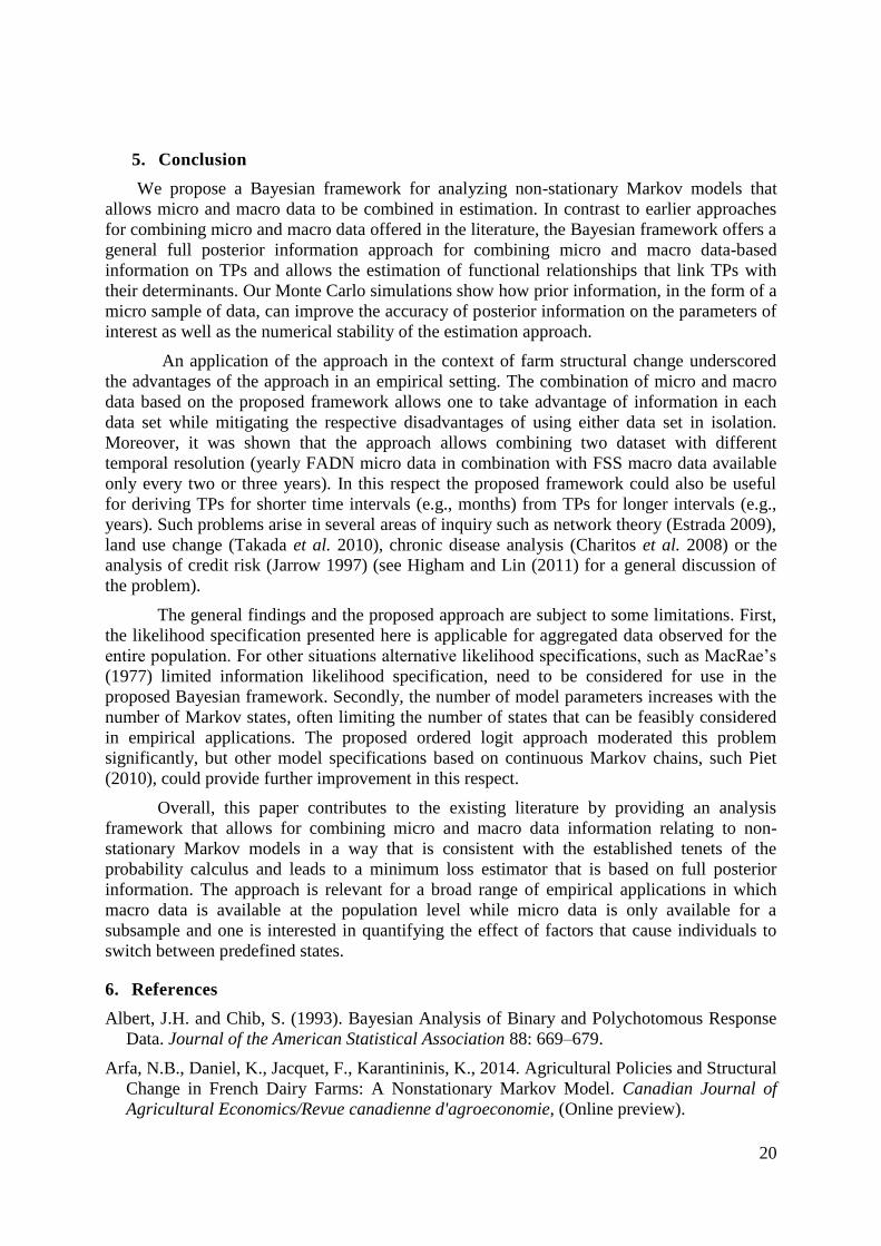
5. Conclusion

We propose a Bayesian framework for analyzing non-stationary Markov models that

allows micro and macro data to be combined in estimation. In contrast to earlier approaches

for combining micro and macro data offered in the literature, the Bayesian framework offers a

general full posterior information approach for combining micro and macro data-based

information on TPs and allows the estimation of functional relationships that link TPs with

their determinants. Our Monte Carlo simulations show how prior information, in the form of a

micro sample of data, can improve the accuracy of posterior information on the parameters of

interest as well as the numerical stability of the estimation approach.

An application of the approach in the context of farm structural change underscored

the advantages of the approach in an empirical setting. The combination of micro and macro

data based on the proposed framework allows one to take advantage of information in each

data set while mitigating the respective disadvantages of using either data set in isolation.

Moreover, it was shown that the approach allows combining two dataset with different

temporal resolution (yearly FADN micro data in combination with FSS macro data available

only every two or three years). In this respect the proposed framework could also be useful

for deriving TPs for shorter time intervals (e.g., months) from TPs for longer intervals (e.g.,

years). Such problems arise in several areas of inquiry such as network theory (Estrada 2009),

land use change (Takada et al. 2010), chronic disease analysis (Charitos et al. 2008) or the

analysis of credit risk (Jarrow 1997) (see Higham and Lin (2011) for a general discussion of

the problem).

The general findings and the proposed approach are subject to some limitations. First,

the likelihood specification presented here is applicable for aggregated data observed for the

entire population. For other situations alternative likelihood specifications, such as MacRae’s

(1977) limited information likelihood specification, need to be considered for use in the

proposed Bayesian framework. Secondly, the number of model parameters increases with the

number of Markov states, often limiting the number of states that can be feasibly considered

in empirical applications. The proposed ordered logit approach moderated this problem

significantly, but other model specifications based on continuous Markov chains, such Piet

(2010), could provide further improvement in this respect.

Overall, this paper contributes to the existing literature by providing an analysis

framework that allows for combining micro and macro data information relating to non-

stationary Markov models in a way that is consistent with the established tenets of the

probability calculus and leads to a minimum loss estimator that is based on full posterior

information. The approach is relevant for a broad range of empirical applications in which

macro data is available at the population level while micro data is only available for a

subsample and one is interested in quantifying the effect of factors that cause individuals to

switch between predefined states.

6. References

Albert, J.H. and Chib, S. (1993). Bayesian Analysis of Binary and Polychotomous Response

Data. Journal of the American Statistical Association 88: 669–679.

Arfa, N.B., Daniel, K., Jacquet, F., Karantininis, K., 2014. Agricultural Policies and Structural

Change in French Dairy Farms: A Nonstationary Markov Model. Canadian Journal of

Agricultural Economics/Revue canadienne d'agroeconomie, (Online preview).

21

Brown, P.J. and Payne, C.D. (1986). Aggregate data, ecological regression, and voting

transitions. Journal of the American Statistical Association 81: 452–460.

Charitos, T., de Waal, P.R., and van der Gaag, L.C. (2008). Computing short-interval

transition matrices of a discrete-time Markov chain from partially observed data. Statistics

in Medicine 27: 905–921.

Chib, S. and Greenberg, E. (1995). Understanding the Metropolis-Hastings Algorithm. The

American Statistician 49: 327–335.

Estrada, E. (2009). Information mobility in complex networks. Physical Review E 80: 026104

1-12.

Frühwirth-Schnatter, S. and Frühwirth, R. (2007). Auxiliary mixture sampling with

applications to logistic models. Computational Statistics & Data Analysis 51: 3509–3528.

Hawkes, A.G. (1969). An Approach to the Analysis of Electoral Swing. Journal of the Royal

Statistical Society: Series A (Statistics in Society) 132: 68–79.

Hawkins, D.L. and Han, C. (2000). Estimating Transition Probabilities from Aggregate

Samples Plus Partial Transition Data. Biometrics 56: 848–854.

Heckelei, T., Mittelhammer, R.C., and Jansson ,T. 2008. A Bayesian Alternative to

Generalized Cross Entropy Solutions for Underdetermined Econometric Models.

Discussion Paper 2008:2, Institute for Food and Resource Economics, University of Bonn.

Higham, N.J. and Lin, L. (2011). On pth roots of stochastic matrices. Linear Algebra and its

Applications 435: 448–463.

Huettel, S., Jongeneel, R. 2011. How has the EU milk quota affected patterns of herd-size

change? European Review of Agricultural Economics 38: 497–527.

Jarrow, R.A. (1997). A Markov model for the term structure of credit risk spreads. Review of

Financial Studies 10: 481–523.

Karantininis, K. 2002. Information-based estimators for the non-stationary transition

probability matrix: an application to the Danish pork industry. Journal of Econometrics

107:275–290.

Lancaster, G.A., Green, M., and Lane, S. (2006). Reducing bias in ecological studies: an

evaluation of different methodologies. Journal of the Royal Statistical Society: Series A

(Statistics in Society) 169: 681–700.

Liu, J.S. (2008). Monte Carlo strategies in scientific computing. New York: Springer.

Liu, J.S., Liang, F., and Wong, W.H. (2000). The Multiple-Try Method and Local

Optimization in Metropolis Sampling. Journal of the American Statistical Association 95:

121–134.

MacRae, E.C. (1977). Estimation of Time-Varying Markov Processes with Aggregate Data.

Econometrica 45: 183–198.

McCarthy, C. and Ryan, T.M. (1977). Estimates of Voter Transition Probabilities from the

British General Elections of 1974. Journal of the Royal Statistical Society. Series A

(General) 140: 78–85.

22

Musalem, A., Bradlow, E.T., and Raju, J.S. (2009). Bayesian estimation of random-

coefficients choice models using aggregate data. Journal of Applied Econometrics 24:

490–516.

Pelzer, B. and Eisinga, R. (2002). Bayesian estimation of transition probabilities from

repeated cross sections. Statistica Neerlandica 56: 23–33.

Piet, L. (2010). A structural approach to the Markov chain model with an application to the

commercial French farms. Paper presented: 4èmes journées de recherches en sciences

sociales, 9-10.12.2010, Rennes, France.

Rosenqvist, G. (1986). Micro and macro data in statistical inference on Markov chains.

Dissertation Swedish School of Economics and Business Administration: Helsingfors.

Scott, S.L. (2011). Data augmentation, frequentist estimation, and the Bayesian analysis of

multinomial logit models. Statistical Papers 52: 87–109.

Takada, T., Miyamoto, A., and Hasegawa, S.F. (2010). Derivation of a yearly transition

probability matrix for land-use dynamics and its applications. Landscape Ecology 25: 561–

572.

Train, K.E. (2009). Discrete choice methods with simulation. New York: Cambridge

University Press.

Upton, G.J.G. (1978). A Note on the Estimation of Voter Transition Probabilities. Journal of

the Royal Statistical Society, Series A (General) 141: 507–512.

Wakefield, J. (2004). Ecological inference for 2×2 tables. Journal of the Royal Statistical

Society: Series A (Statistics in Society) 167: 385–445.

Zimmermann, A. and Heckelei, T. (2012a). Structural Change of European Dairy Farms – A

Cross regional Analysis. Journal of Agricultural Economics, 63: 576-603.

Zimmermann, A., Heckelei, T. 2012b. Differences of farm structural change across European

regions. Discussion Paper 2012:4, Institute for Food and Resource Economics, University

of Bonn.

Zimmermann, A., Heckelei, T., and Domínguez, I.P. (2009). Modelling farm structural

change for integrated ex-ante assessment: review of methods and determinants.

Environmental Science & Policy 12: 601–618.

23

7. Appendix

Appendix A1: Number of farms (in 1000) observed in the FSS dataset and fitted values of the Markov

multinomial logit model. Results aggregated over all considered regions and differentiated between the five

different farm types and the total number of farms.

1990 1995 2000 20050

5

10

15

20

25 FSS Fitted

COP Crop

1990 1995 2000 20050

10

20

30

Other Crop

1990 1995 2000 20050

20

40

60

80

100Milk

1990 1995 2000 20050

2

4

6

8

10

12

14

16 Other Livestock

1990 1995 2000 20050

10

20

30

40

50

60

70 Mix

1990 1995 2000 20050

50

100

150

200

Total Number of Farms

24

Appendix A2: Number of farms (in 1000) observed in the FSS dataset and fitted values of the Markov ordered

logit model. Results aggregated over all considered regions and differentiated between the three different size

classes and the total number of farms. The figures illustrate that fitted values follow closely the observed FSS

macro data available every 2-3 years. Additionally to approach provides a direct prediction of macro data for

years between FSS years.

1990 1995 2000 20050

20

40

60

80

100

120

140 FSS Fitted

Small

1990 1995 2000 20050

20

40

60

80

Medium

1990 1995 2000 20050

5

10

15

20

25

30

35 Large

1990 1995 2000 20050

50

100

150

200

Total farm

bayesian estimation of non-stationary markov models...

Documents