bayestraits v2 (beta, unfinished) july 2013beta).pdf · 2014-06-02 · bayestraits v2 (beta,...

BayesTraits V2 (Beta, unfinished)

July 2013

Mark Pagel ([email protected])

Andrew Meade ([email protected])

TableofContentsMajor Changes from V1 .......................................................................................................................... 4

Introduction ............................................................................................................................................ 4

Methods and Approach .......................................................................................................................... 4

BayesTraits methods ............................................................................................................................... 5

Tree Format ............................................................................................................................................ 5

Data Format ............................................................................................................................................ 5

Running BayesTraits ................................................................................................................................ 6

Running BayesTraits with a command file .......................................................................................... 7

Continuous‐time Markov models of trait evolution for discrete traits .................................................. 7

The Generalised Least Squares model for continuously varying traits ................................................... 8

Hypothesis Testing: Likelihood ratios and Bayes Factors ....................................................................... 9

Priors ..................................................................................................................................................... 10

Burn‐in and sampling in MCMC analysis ............................................................................................... 11

The parameter proposal mechanism and mixing in MCMC analysis .................................................... 11

Mixing................................................................................................................................................ 11

AutoTune .......................................................................................................................................... 11

Monitoring Acceptance Rate ............................................................................................................ 12

Over parameterisation .......................................................................................................................... 12

Parameter restriction ........................................................................................................................ 12

Reverse Jump MCMC ........................................................................................................................ 13

Multistate ML example ......................................................................................................................... 13

Multistate MCMC example ................................................................................................................... 14

Parameter restriction example ............................................................................................................. 14

Ancestral state reconstruction Multistate / discrete ............................................................................ 15

Fixing node values / fossilising .............................................................................................................. 16

Discrete examples ................................................................................................................................. 17

Discrete independent ........................................................................................................................... 17

Discrete dependent .............................................................................................................................. 18

Reverse Jump MCMC and mode reduction .......................................................................................... 19

Covarion model ..................................................................................................................................... 20

Continuous: Random Walk (Model A) ML ............................................................................................ 20

Continuous: Random Walk (Model A) MCMC ...................................................................................... 21

Testing trait correlations: continuous ................................................................................................... 21

Continuous: Directional (Model B) MCMC ........................................................................................... 22

Continuous: Regression ........................................................................................................................ 22

Testing trait significance ................................................................................................................... 22

Tree transformations, kappa, lambda, delta ........................................................................................ 22

Continuous: Estimating unknown values .............................................................................................. 24

Example: Estimating unknown values internal nodes ...................................................................... 24

Example: Estimating unknown values for tips .................................................................................. 25

Independent contrast ........................................................................................................................... 26

Variable rates model ............................................................................................................................. 26

Command List ....................................................................................................................................... 27

Common problem / Frequently Asked Questions ................................................................................ 34

References ............................................................................................................................................ 35

MajorChangesfromV1 Rate deviation and data deviation parameters are automatically tuned

Hard polytomys are now supported

A range of new models:

Multiple regression

Variable rates

Independent contrast

Covarion

Improved handling of model files

Estimation of internal and tips for continuous models

Numerous bug fixes and improvements

Note: Trees are now normalised to have a mean branch length of 0.1 for discrete and

multistate models, rate estimates will change from V1 to V2 but will be relatively comparable.

IntroductionBayesTraits is a computer package for performing analyses of trait evolution among groups

of species for which a phylogeny or sample of phylogenies is available. It can be applied to the

analysis of traits that adopt a finite number of discrete states, or to the analysis of continuously

varying traits. Hypotheses can be tested about models of evolution, about ancestral states and

about correlations among traits. The method can be used to take into account uncertainty about the

model of evolution and the underlying phylogeny.

MethodsandApproachBayesTraits uses Markov chain Monte Carlo (MCMC) methods to derive posterior

distributions and maximum likelihood (ML) methods to derive point estimates of, log‐likelihoods, the

parameters of statistical models, and the values of traits at ancestral nodes of phylogenies. The user

can select either standard or conventional MCMC or reversible‐jump MCMC. In the latter case the

Markov chain searches the posterior distribution of different models of evolution as well as the

posterior distributions of the parameters of these models (see below).

BayesTraits can be used with a single phylogenetic tree in which case only uncertainty about

model parameters is explored, or, it can be applied to suitable samples of trees such that models are

estimated and hypotheses are tested taking phylogenetic uncertainty into account.

Our BayesPhylogenies package (www.evolution.reading.ac.uk) can be used to generate

posterior distributions of phylogenetic trees when a gene‐sequence alignment or other data set is

available.

BayesTraitsmethods• MultiState is used to reconstruct how traits that adopt a finite number of discrete states

evolve on phylogenetic trees. It is useful for reconstructing ancestral states and for testing models

of trait evolution. It can be applied to traits that adopt two or more discrete states (see Pagel, M.,

Meade, A. and Barker, D. 2004. Systematic Biology, 53, 673‐684;

• Discrete is used to analyse correlated evolution between pairs of discrete binary traits. Most

commonly the two binary states refer to the presence or absence of some feature, but could also

include “low” and “high”, or any two distinct features. Its uses might include tests of correlation

among behavioural, morphological, genetic or cultural characters (see Pagel, M. and Meade, A.

2006. American Naturalist, 167, 808‐825.)

• Continuous is for the analysis of the evolution of continuously varying traits. It can be used

to model the evolution of a single trait, to study correlations among pairs of traits, or to study the

regression of one trait on two or more other traits (see Pagel, M. 1999. Nature, 401, 877‐884).

• Continuous regression is used to build regression models and use these models to

reconstruct past values (ref)

• Variable rates is used to detect variations in the rate of evolution threw the tree, accounting

for change in rate on a single lineage or for a group of taxa. (ref)

This manual is designed to show how to use the programs that implement these models. Detailed

information about the methods can be found in the papers listed at the end (some are available as

pdfs on our website). Syntax and a description of all of the commands in BayesTraits are listed

below.

TreeFormat BayesTraits requires trees to be in Nexus format, trees can now include hard polytomy but

must be correctly rooted and include branch lengths. Taxa names must not be included in the

description of the tree but should be linked to a number in the translate section of the tree file, a

number of example trees are included with the program.

DataFormat Data is read from a plain text file (ASCII), with one line for each species or taxon in the tree.

The names must be spelled exactly as in the trees and must not have any spaces within them. They

do not have to be in the same order. Following a species name, leave white space (tab or space) and

enter the first column of data, repeat this for additional columns of data. Data for MultiState

analysis should take values such as “0”, “1”, “2” or “A”, “B”, “C” etc. Discrete data must be exactly

two columns of binary data and must take the values “0” or “1”. Continuous data should be integers

or floating points. If data is missing it should be represented using “‐“, for a trait in MultiState or

Discrete the remaining data for the taxa is used, if data is missing for continuous the taxa is removed

from the tree. Example data files for MultiState, Discrete and Continuous data are included with the

program.

Example of MultiState data

Taxon01 A A C

Taxon02 B B C

Taxon03 A B ‐

Taxon04 C C B

….

TaxonN BC A B

Taxon 3 has missing data for the third site. Missing data are treated as if the trait could take

any of the other states. The first trait for Taxon n is uncertain. The code BC signifies that it can be in

states B or C (with equal probability) but not in state A.

Example of Discrete (binary) data

Taxon01 0 0

Taxon02 0 ‐

Taxon03 1 0

Taxon04 0 1

….

TaxonN 1 1

Example of Continuous data

Taxon01 10 9.0

Taxon02 1.06 ‐

Taxon03 5.3 2

Taxon04 3 4

….

TaxonN 1 1.1

RunningBayesTraits BayesTraits is run from the command prompt (windows) or terminal (OS X and Linux), it is

not run by double clicking on it. The program, tree file and data file should be place in the same

directory / folder. Start the command prompt / terminal and change to the directory the program,

tree and data is in and type.

Windows

BayesTraits.exe TreeFile DataFile

Linux / OSX

./BayesTraits TreeFile DataFile

Where TreeFile is the name of the tree file and DataFile is the name of the data file.

RunningBayesTraitswithacommandfile If you need to run an analysis multiple times or if it is complex it can be more convenient to

place the commands into a command file, instead of typing them in each time. A command file is a

plane ASCII text file, with the commands to run.

An example command file is included with the program, “ArtiodactylMLIn.txt”. The file has

three lines,

1 1

run The first line selects MultiState, the second is for ML analysis and the third is to run the

program. To run BayesTraits using the Artiodacty tree, data and input file use the following command.

Windows

BayesTraits.exe Artiodactyl.trees Artiodactyl.txt < ArtiodactylMLIn.txt

Linux / OS X

./BayesTraits Artiodactyl.trees Artiodactyl.txt < ArtiodactylMLIn.txt

Continuous‐timeMarkovmodelsoftraitevolutionfordiscretetraitsMultistate and Discrete fit continuous‐time Markov models to discrete character data. This model

allows the trait to change from the state it is in at any given moment to any other state over infinitesimally

small intervals of time. The rate parameters of the model estimate these transition rates (see Pagel, 1994 for

further discussion). The model traverses the tree estimating transition rates and the likelihood associated with

different states at each node.

The table below shows an example of the model of evolution for a trait that can adopt three states, 0,

1, and 2. The qij are the transition rates among the three states, and these are what the method estimates on

the tree, based on the distribution of states among the species. If these rates differ from zero, this indicates

that they are a significant component of the model. The main diagonal elements are not estimated but are a

function of the other values in their row.

Example of the model of evolution for a trait that adopts three states

State 0 1 2

0 ‐‐ q01 q02

1 q01 ‐‐ q12

2 q20 q21 ‐‐

For a trait that adopts four states, the matrix would have twelve entries, for a binary trait the matrix

would have just two entries.

Discrete tests for correlated evolution in two binary traits by comparing the fit (log‐likelihood) of two

of these continuous‐time Markov models. One of these is a model in which the two traits evolve

independently on the tree. Each trait is described by a 22 matrix in the same format as the one above, but in

which the trait adopts just two states, “0” and “1”. This creates two rate coefficients per trait.

The other model, allows the traits to evolve in a correlated fashion such that the rate of change in one

trait depends upon the background state of the other. The dependent model can adopt four states, one for

each combination of the two binary traits (0,0; 0,1; 1,0; 1,1). It is represented in the program as shown below

and the transition rates describe all possible changes in one state holding the other constant. The main

diagonal elements are estimated from the other values in their row as before. The other diagonal elements

are set to zero as the model does not allow ‘dual’ transitions to occur, the logic being that these are

instantaneous transition rates and the probability of two traits changing at exactly the same instant of time is

negligible. Dual transitions are allowed over longer periods of time, however. See Pagel (1994) and Barker

and Pagel (2005) for further discussion of this model.

State 0,0 0,1 1,0 1,1

0,0 ‐‐ q12 q13 ‐‐

0,1 q21 ‐‐ ‐‐ q24

1,0 q31 ‐‐ ‐‐ q34

1,1 ‐‐ q42 q43 ‐‐

The values of the transition rate parameters will depend upon the units of measurement in the

phylogeny. In general if the branch lengths are increased by a factor ‘c’ the transition rates will be decreased

by the same factor ‘c’. This has implications for modelling the rate parameters in Markov chains as discussed

below.

Covarion model. BayesTraits implements the covarion model for trait evolution (Tuffley and Steele,

Math. Biosci. 147:63–91, 1998). This is a variant of the continuous‐time Markov model that allows for traits to

vary their rate of evolution within and between branches. It is an elegant model that deserves more attention,

although users may find it of limited value with comparative data – the model may require many sites to be

estimated well.

TheGeneralisedLeastSquaresmodelforcontinuouslyvaryingtraitsContinuous analyses phylogenetically structured continuously varying data using a generalised least

squares (GLS) approach that assumes a Brownian motion model of evolution (see Pagel, 1997, 1999). In the GLS model, non‐independence among the species is accounted for by reference to a matrix of the expected covariances among species. This matrix is derived from the phylogenetic tree. The model estimates the variance of evolutionary change (the Brownian motion parameter), sometimes called the ‘rate’ of change, and the ancestral state of traits at the root of the tree. It can also estimate the covariance of changes between pairs of traits, and this is how it tests for correlation.

The GLS approach means that data can be plotted across species and interpreted using the correlations and regressions obtained from Continuous. The GLS approach as implemented in Continuous also makes it possible to transform and scale the phylogeny to test the adequacy of the underlying model of

evolution, to assess whether phylogenetic correction of the data is required, and to test hypotheses about trait evolution itself – for example, is trait evolution punctuational or gradual, is there evidence for adaptive radiation, is the rate of evolution constant.

HypothesisTesting:LikelihoodratiosandBayesFactorsBayesTraits does not test hypotheses for you but prints out the information needed to make

hypothesis tests. These will be discussed in more detail in conjunction with the examples below, but here we

outline the two kinds of tests most often used.

The likelihood ratio (LR) test is often used to compare two likelihoods derived from nested model

(models that can be expressed such that one is a special or general case of the other). The likelihood ratio

statistic is calculated as

LR= 2[log‐likelihood(better fitting model) – log‐likelihood(worse fitting model)]

The likelihood ratio statistic is nominally distributed as a 2 with degrees of freedom equal to the

difference in the number of parameters between the two models. However, in some circumstances (see Pagel,

1994, 1997 and Barker and Pagel, 2005) the test may follow a 2 with fewer degrees of freedom.

Variants of the LR test include the Akaike Information Criterion and the Bayesian Information

Criterion. We do not describe these tests here. They are discussed in many works on phylogenetic inference

(see for example, Felsenstein. Inferring Phylogenies, 2004).

The LR, Akaike and Bayesian Information Criterion tests presume that the likelihood is at or near its

maximum likelihood value. In a MCMC framework tests of likelihood often rely on Bayes factors. The logic is

similar to that for the likelihood ratio test, except here we compare the marginal likelihoods of two models

rather than their maximum likelihoods.

The marginal likelihood of a model is the integral of the model likelihoods over all values of the

models parameters and over possible trees. In practice this marginal likelihood is difficult to estimate but

research shows it can be well approximated by the harmonic mean of the likelihoods allowing the Markov

chain to run for a very large number of iterations (millions). It is important to check that the harmonic mean is

well estimated.

BayesTraits calculates the logarithm of the harmonic mean of the likelihoods as the program runs,

having ignored the likelihoods during the burn‐in period when the model is moving to convergence. The

running tally of harmonic means is read from the final iteration of the chain and the values for the

independent and dependent models are then compared. As the harmonic mean is a running total, only the last

harmonic mean is used. The test statistic is just

Log BF = 2(log[harmonic mean(complex model)] – log[harmonic mean(simple model)]

Log Bayes factor Interpretation

<2 Weak evidence

>2 Positive evidence

5‐10 Strong evidence

>10 Very strong evidence

Model testing is a controversial topic with Bayesian analysis, and other options such as BIC, AIK, DIC may be considered.

PriorsWhen using MCMC analysis method, the prior distributions of the parameters of the model of

evolution must be chosen. The values of the rate parameters are dependent upon the branch lengths of the

tree. Other things equal, longer branches will require smaller rate parameters and vice versa. This is why the

user must set the kind of prior (e.g., uniform, exponential) and the prior‐interval or range of values the prior

covers.

Uniform or uninformative priors should be used if possible as these assume all values of the

parameters are equally likely a priori and are therefore easily justified. Uniform priors can be used when the

signal in the data is strong. But in a comparative study there will typically only be one or a few data points

(unlike the many hundreds or thousands in a typical gene‐sequence alignment) and so a stronger prior than a

uniform may be required.

Priors are the soft underbelly of Bayesian analyses. The guiding principle is that if the choice of prior

is critical for a result, you must have a good reason for choosing that prior. It is often useful to run maximum

likelihood analyses on your trees to get a sense of the average values of the parameters. One option if a

uniform with a wide interval does not constrain the parameters is to use a uniform prior with a narrower range

of values, and this might be justified either on biological grounds or perhaps on the ML results. The ML results

will not define the range of the prior but can give an indication of its midpoint.

NOTE: A rule of thumb when choosing a constrained or informed (non‐uniform) prior is that if the posterior

distribution of parameter values seems truncated at either the upper or lower end of the constrained range,

then the limits on the prior must be changed.

The program allows uniform, exponential, gamma and beta distributed priors. The exponential

distribution always has its mode at zero and then slopes down, whereas the gamma can take a variety of uni‐

modal shapes or even mimic the exponential. The exponential prior is useful when the general feeling is that

smaller values of parameters are more likely than larger ones. If the parameters are thought to take an

intermediate value, a gamma prior with an intermediate mean can be used.

Priors are set using the prior command, the Prior command takes a parameter to set the prior for, a

distribution (uniform, exp, gamma or beta) and the parameters of the distribution.

Prior q01 exp 10

Is used to set an exponential prior with a mean of 10 for the rate parameter q01

Prior q10 uniform 0 100

Set the prior on q10 to a uniform 0 – 100

In many cases you will want to use the same prior on all parameters, the PriorAll command can be

used to set all prior the same. It is identical to the prior command but does not take a parameter.

Because it can be difficult to arrive at suitable values for the parameters of the prior distributions,

BayesTraits allows the use of a hyper prior. A hyper prior is simply a distribution – usually a uniform ‐‐ from

which are drawn values to seed the values of the exponential or gamma priors. We recommend using

hyperpriors as they provide an elegant way to reduce some of the uncertainty and arbitrariness of choosing

priors in MCMC studies. For an example of selecting priors and using a hyper prior see Pagel, M., Meade, A.

and Barker, D. 2004 Bayesian estimation of ancestral character states on phylogenies. Systematic Biology, 53,

673‐684.

When using the hyper prior approach you specify the range of values for the uniform distribution that

is used to seed the prior distribution. Thus, for example HyperPriorAll exponential 0 10 seeds the mean of the

exponential prior from a uniform on the interval 0 to 10. HyperPriorAll gamma 0 10 0 10 seeds the mean and

variance of the gamma prior from uniform hyper priors both on the interval 0 to 10.

Burn‐inandsamplinginMCMCanalysisThe burn‐in period of a MCMC run is the early part of the run while the chain is reaching

convergence. It is impossible to give hard and fast rules for how many iterations to give to burn‐in.

We often find that a minimum of 10,000 and seldom more than 500,000 is sufficient. The length of

burn‐in is set with the burnin command. During burn‐in nothing is printed out. More complex

models or larger trees may require longer burn‐in periods.

Because successive iterations of most Markov chains are auto correlated, there is frequently

nothing to be gained from printing out each line of output. Instead the chain is sampled or thinned

to ensure that successive output values are roughly independent. This is the job of the sample

command. It instructs the program only to print out every nth sample of the chain. Choose this

value such that the autocorrelation among successive points is low (this can be checked in most

statistics programs or even Excel). For many comparative datasets, choosing every 1000th or so

iteration is more than adequate to achieve a low autocorrelation.

The chain is run for 1010000 iterations by default, this can be changed with the iterations

command, which takes the number of iterations to run for or ‐1 for an infinite chain, which can be

stopped by holding Ctrl and pressing C.

TheparameterproposalmechanismandmixinginMCMCanalysis

MixingMixing, how many times a proposed change to a chain is accepted, is key to a successful

MCMC analysis. If changes to a parameter are too large the likelihood will change dramatically, and at convergence many of the proposed changes will have a poor likelihood. This will cause the chain to mix poorly, resulting in a low acceptance rate and the chain becoming stuck, where between samples no other solution is accepted. The other side of the coin is, if to small changes are propose the likelihood does not change much, leading to a high acceptance rate, causing the chain to wonder. An ideal acceptance rate is between 20‐40% at convergence.

Parameter value can vary widely between data sets and trees, parameters obtained from an of a molecular tree using body size data, may be many orders of magnitude different from parameters obtained using a time tree in millions of years using genome size. This makes it very hard to find a universal proposal mechanism. The rate deviation parameter (RateDev) controls the size of change to use. Large rate deviation values make bigger changes leading to lower acceptance rates, small values lead to higher acceptance rates. Non‐continuous parameters such as the tree used or reverse jump acceptance rate, cannot be tuned.

AutoTuneBy default BayesTraits attempts to automatically tune the proposal mechanism to find a rate

deviation parameter which gives and acceptance rate of approximately 30% but this can be

overridden using the RateDev command. The command takes a number, for example the command below sets the rate deviation to 8.5

RateDev 8.5

MonitoringAcceptanceRateBayesTraits produces a schedule file which is used to monitor how the chain is mixing, the

file contains the schedule, the percentage of operators tried, followed by a header. The header shows the number of times an operator was tried and the percentage of time it was accepted, if auto tune is used the rate dev values, acceptance rate for that parameter, the average acceptance for that iteration and the running mean acceptance rate is recorded. The schedule file should be reviewed to make sure the chain is mixing correctly.

OverparameterisationThere is a constant battle in comparative methods between model complexity and data

needed to estimate parameters. In many case, especially with multistate and discrete data, the model will require too many parameters, which cannot be estimated with the available data. This causes the model to be over parameterised. Indications of over parameterisation include, poorly estimated parameters, parameters trading off with each other, suboptimal likelihoods, and poor convergence / parameter optimisation. Model complexity can be reduced by combining parameters with the restrict command and ensuring the ratio of parameters to data is not high.

ParameterrestrictionThe default multistate and discrete models are often over parameterised, due to the large

number of parameters, many of which may not be supported. BayesTraits allows parameters to be restricted to each other, this is used to reduce the number of free parameters and increase the information available to estimate the remaining ones. The restrict command (res) is used to restrict parameter, the command takes two or more parameter names, restricting all supplied parameters to the first

To restrict alpha2 to alpha1 use the following command Res alpha1 alpha2

To restrict all parameters, in an independent model, to alpha 1 use Res alpha1 alpha2 beta1 beta2 Or ResAll alpha1

Parameters can also be restricted to constants, including zero, in the same way Res alpha1 1.5 Or Res alpha1 alpha2 1.5

The unrestricted (UnRes) command can be used remove restrictions Model testing (see above) can be used to test if a parameter is statistically justified, when

rates are restrict the number of free parameters is reduced.

ReverseJumpMCMC For a complex model the number of possible restrictions is large, and may be impossible to

test. A reverse jump MCMC method was developed to integrate result over model parameter and

model restrictions, for a detailed description see (ref).

The RevJump (RJ) command is used to select revers jump MCMC, the command take a prior

and prior parameters. For example, the command below uses reverse jump with an exponential

prior with a mean of 10. The second command uses reverse jump with a hyper exponential prior

drawn from a uniform 0 ‐ 100

RevJump exp 10 Or RJHP exp 0 100

MultistateMLexample

Start the program using the “Artiodactyl.trees” tree file and the “Artiodactyl.data” file. The following screen should be presented to you

Please Select the model of evolution to use. 1) MultiState

Select 1 for the MultiState model

Please Select the analysis method to use. 1) Maximum Likelihood. 2) MCMC

Select 1 for maximum likelihood analysis. The default options will be printed, displaying basic information. This should always be checked to ensure it is what you expect. Type run The analysis will start. The options for the run will be printed followed by a header row. The header row is the

Header Output

Tree No The tree number, 1‐500 for this data

Lh Maximum likelihood value for the tree

qDG The transition rate from D to G

qGD The transition rate from G to D

Root P(D) The probability the root is in state D

Root P(G) The probability the root is in state G

For each tree in the sample a line of output will be printed. Once all trees have been analysed the program will terminate.

MultistateMCMCexampleStart the program using the “Artiodactyl.trees” tree and “Artiodactyl.data” data file, select

multistate (1) and MCMC (2). The default options will be printed.

Set all priors to an exponential with a mean of 10, and start the chain, using PriorAll exp 10 Run

A header will be printed Header Output

Iteration Current iteration of the chain

Lh Current likelihood of the chain

Harmonic Mean Running harmonic mean

Tree No Current tree number

qDG Transition rate from D to G

qGD Transition rate from G to D

Root P(D) Probability the root is in state D

Root P(G) Probability the root is in state G

Iteration Lh Harmonic Mean

Tree No qDG qGD Root P(D)

Root P(G)

11000 ‐7.93307 ‐7.93307 187 3.702561 2.5446 0.351023 0.648977

12000 ‐8.98846 ‐8.59398 495 3.120973 4.914959 0.475628 0.524372

13000 ‐8.37416 ‐8.52594 99 3.799383 4.489798 0.417393 0.582607

14000 ‐10.2806 ‐9.31231 95 17.07613 27.54498 0.499972 0.500028

15000 ‐10.7122 ‐9.78912 95 6.945588 5.865219 0.48436 0.51564

… … … … … … … …

1006000 ‐8.94481 ‐9.90388 400 8.97661 8.407563 0.473517 0.526483

1007000 ‐8.53244 ‐9.90313 147 0.33644 1.477702 0.012116 0.987884

1008000 ‐8.03562 ‐9.90228 338 2.454093 3.334973 0.270869 0.729131

1009000 ‐8.41139 ‐9.90151 107 2.217407 4.183507 0.365974 0.634026

1010000 ‐9.72812 ‐9.90135 61 7.50541 9.538785 0.484114 0.515886

Output from the chain is tab separated and is designed to be using in program such as excel

and JMP. Run to run output will vary and is depend on the random seed used.

The scheduled file “Artiodactyl.txt.Schedule.txt” will be created, this should be check to

ensure the chain is mixing correctly.

Parameterrestrictionexample

The previous example assumed that the transition rate between qDG and qGD were

different and estimated both separately. To test if qDG and qGD are significantly different from each

other, re‐run the analysis restricting qGD to take the same value qDG. The same restrict command

can be used in ML analysis.

PA exp 10 Restrict qDG qGD Run

The output should be very similar but the rate parameters qDG and qGD should be the same

each iteration. The significance of the test can be found by calculating a Bayes Factor from the

harmonic means.

The harmonic mean from the analysis where qDG ≠ qGD = ‐9.90135, the harmonic mean

where qDG = qGD = ‐8.965492. The complex model is qDG ≠ qGD, because it has one more

parameter than the simple model, qDG = qGD. The Bayes Factor (BF) is given as

Log BF = 2(log[harmonic mean(complex model)] – log[harmonic mean(simple model)] Log BF = 2(‐9.90135 ‐ ‐8.965492) Log BF = ‐1.871716 As the BF is less than two the simpler model should be favoured

Note: Values of the harmonic means will vary between runs depending on the random seed

and how long the chain is run for, values are only for illustrative purposes. The harmonic means

were calculated from a very short run and were not tested for reliability using multiple independent

and longer runs. They are only used to demonstrate basic model testing.

AncestralstatereconstructionMultistate/discrete

The AddMRCA and AddNode commands are used to reconstruct ancestral states in multistate and discrete models. The syntax for the two commands are similar. The commands take a tag which is used to identify the node in the output, and a list of taxa names or taxa number which define the node. BayesTrees (see website) is a graphics tree viewer which can be used to generate the command by clicking on the appropriate node. Using the “Artiodactyl.trees” tree and “Artiodactyl.data”, select multistate and MCMC The two commands below add a node to reconstruct, defined by Porpoise Dolphin FKWhale and Whale. The node is called “Node1”. The second command is identical but uses the taxa number instead of taxa names to define the node.

AddNode Node1 Porpoise Dolphin FKWhale Whale AddNode Node1 5 6 7 8

run the program with the following commands

PA exp 10 Res qDG qGD AddNode Node1 Porpoise Dolphin FKWhale Whale Run

Two new columns should be added to the output “Node1 P(D)” and “Node1 P(G)”, these represent the probability of reconstructing a D or a G at Node1.

BayesTraits uses a sample of trees and not all nodes will be present in all trees, the node defined by Sheep, Goat, Cow, Buffalo and Pronghorn is only present in 58% of the trees. If the commands below are run

PA exp 10 Res qDG qGD AddNode VarNode Sheep Goat Cow Buffalo Pronghorn Run

The posterior probability of node reconstruction will not be present for all samples, some samples will be recorded as “‐‐“ because the node is not present in those trees.

The MRCA command reconstructs the Most Recent Common Ancestor, which will be present in all trees. Rerun the analysis using MRCA.

PA exp 10 Res qDG qGD AddMRCA VarNode Sheep Goat Cow Buffalo Pronghorn Run

Any number of nodes can be reconstructed in a single analysis without any effect on each other.

Fixingnodevalues/fossilising Internal nodes can be set to take a fixed value, if external information is available or to test if the value of one state is significant. The fossil command takes a node name, a state to fossilise in and a list of taxa which define the node, nodes are found using the most recent common ancestor method. The command below fossilises a node defined by sheep, goats, cows, buffalo and pronghorn to state D.

Fossil Node01 D Sheep Goat Cow Buffalo Pronghorn

To test if a fossilised state is significant, run an analysis fossilising a node in one state and compare the results when the node is fossilised in an alternative state. Fossilising states in discrete requires a number instead of a state. The table below show the numbers and there corresponding states. X denotes the likelihood is left unchanged, ‐ set the likelihood to zero.

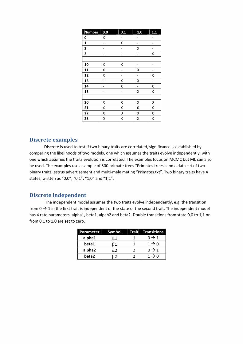
Number 0,0 0,1 1,0 1,1

0 X ‐ ‐ ‐

1 ‐ X ‐ ‐

2 ‐ ‐ X ‐

3 ‐ ‐ ‐ X

10 X X ‐ ‐

11 X ‐ X ‐

12 X ‐ ‐ X

13 ‐ X X ‐

14 ‐ X ‐ X

15 ‐ ‐ X X

20 X X X 0

21 X X 0 X

22 X 0 X X

23 0 X X X

Discreteexamples Discrete is used to test if two binary traits are correlated, significance is established by

comparing the likelihoods of two models, one which assumes the traits evolve independently, with

one which assumes the traits evolution is correlated. The examples focus on MCMC but ML can also

be used. The examples use a sample of 500 primate trees “Primates.trees” and a data set of two

binary traits, estrus advertisement and multi‐male mating “Primates.txt”. Two binary traits have 4

states, written as “0,0”, “0,1”, “1,0” and “1,1”.

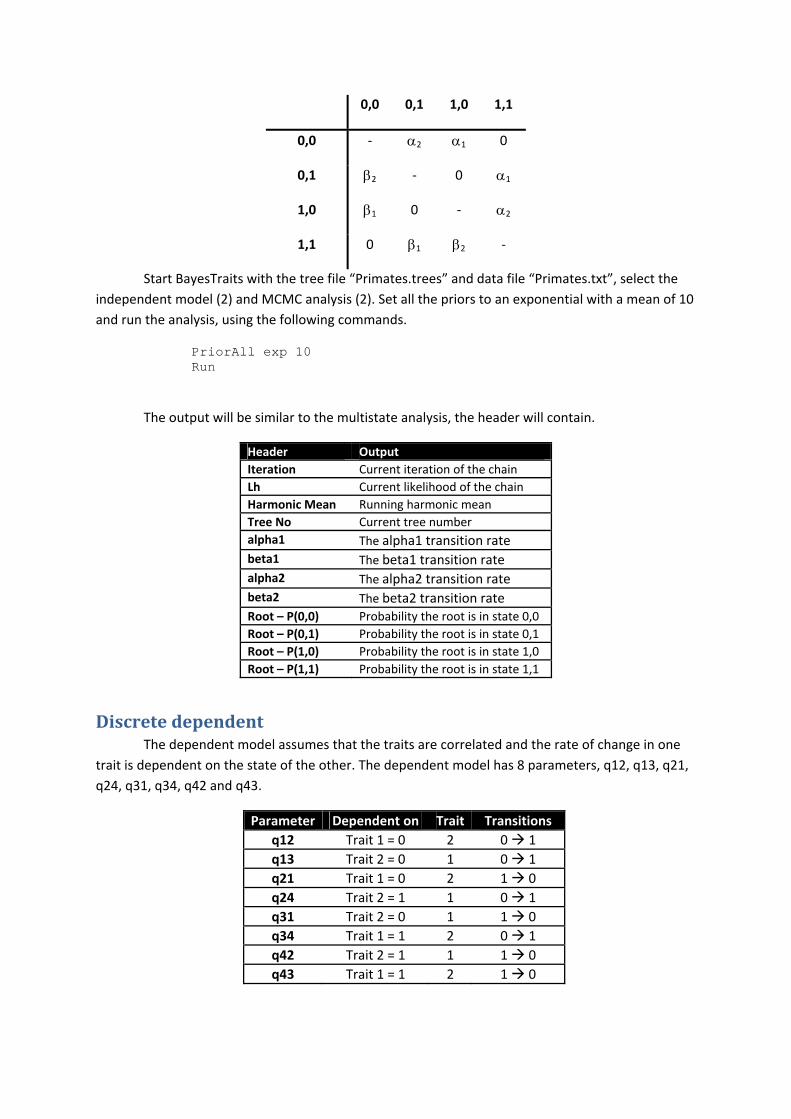
Discreteindependent The independent model assumes the two traits evolve independently, e.g. the transition

from 0 1 in the first trait is independent of the state of the second trait. The independent model

has 4 rate parameters, alpha1, beta1, alpah2 and beta2. Double transitions from state 0,0 to 1,1 or

from 0,1 to 1,0 are set to zero.

Parameter Symbol Trait Transitions

alpha1 1 1 0 1

beta1 1 1 1 0

alpha2 2 2 0 1

beta2 2 2 1 0

0,0 0,1 1,0 1,1

0,0 ‐ 2 1 0

0,1 2 ‐ 0 1

1,0 1 0 ‐ 2

1,1 0 1 2 ‐

Start BayesTraits with the tree file “Primates.trees” and data file “Primates.txt”, select the

independent model (2) and MCMC analysis (2). Set all the priors to an exponential with a mean of 10

and run the analysis, using the following commands.

PriorAll exp 10 Run

The output will be similar to the multistate analysis, the header will contain.

Header Output





alpha1 The alpha1 transition rate beta1 The beta1 transition rate alpha2 The alpha2 transition rate beta2 The beta2 transition rate Root – P(0,0) Probability the root is in state 0,0

Root – P(0,1) Probability the root is in state 0,1



Discretedependent The dependent model assumes that the traits are correlated and the rate of change in one

trait is dependent on the state of the other. The dependent model has 8 parameters, q12, q13, q21,

q24, q31, q34, q42 and q43.

Parameter Dependent on Trait Transitions

q12 Trait 1 = 0 2 0 1

q13 Trait 2 = 0 1 0 1

q21 Trait 1 = 0 2 1 0

q24 Trait 2 = 1 1 0 1

q31 Trait 2 = 0 1 1 0

q34 Trait 1 = 1 2 0 1

q42 Trait 2 = 1 1 1 0

q43 Trait 1 = 1 2 1 0

0,0 0,1 1,0 1,1

0,0 ‐ Q1,2 Q1,3 0

0,1 Q2,1 ‐ 0 Q2,4

1,0 Q3,1 0 ‐ Q3,4

1,1 0 Q4,2 Q4,3 ‐

Start BayesTraits with the tree file “Primates.trees” and data file “Primates.txt”, select the

dependent model (3) and MCMC analysis (2). Set all the priors to an exponential with a mean of 10

and run the analysis, using the following commands.

PriorAll exp 10 Run

The output will be very similar to the independent model except that the dependent

parameters are estimated instead of the independent.

To test if the traits are correlated calculate a Bayes Factor between the independent and

dependent models. If the independents harmonic mean is ‐45.51 and the dependent harmonic mean

is ‐42.47

Log BF = 2(log[harmonic mean(complex model)] – log[harmonic mean(simple model)]

Log BF = 2(‐42.47 ‐ ‐45.51) Log BF = 6.08

The Log BF of 6 suggests there is strong evidence for correlated evolution. Harmonic means will vary between runs but the values should be close.

ReverseJumpMCMCandmodereduction Given the size of the data and complexity of the model it is unlikely that all parameters in

the independent and dependent models are well estimated and statistically distinct. The previous

parameter restriction example, demonstrated how a model could be simplified by restricting

parameters and how to test if restrictions were significant. There are 51 possible restrictions for the

independent model and over 21,000 for the dependent model. Reverse jump MCMC (RJ‐MCMC)

integrates results over the model space, automatically select viable models and parameters.

The reverse jump command takes a prior as a parameter, the command below uses an RJ

MCMC model with an exponential prior with a mean of 10

RJ exp 10

RJ MCMC can also be used with a hyper prior.

RJHP exp 0 100

Run the primates data and tree, with the dependent model and MCMC analysis, using the

commands below

RJ exp 10 Run

The output will contain 4 new columns.

Header Output

No Of Parameters Number of parameters

No Of Zero Number of parameters set to zero

Model string A model string showing parameter restrictions

Dep / InDep A flag showing if the model is dependent (D) or independent (I)

Model strings are used to characterise the models restrictions, the string start with ' and is followed

by numbers indicating which parameters are in which groups or Z if the parameters are been restricted to

zero. For example the modelling string for a dependent model will have 8 sections one for each parameter, the

model string “'1 Z 0 0 0 1 1 Z”, has two parameters and two rates set to zero. The first group consists of the 1st,

6th and 7th parameters (q12, q34 and q42), the second group is formed of the 3rd, 4th and 5th parameters (q21,

q24 and q31), and the 2nd and 8th parameter is set to zero. This can be checked against the parameter

estimates.

To test if a data set is correlated run an independent model using RJ MCMC and compare harmonic

means with a dependent model using RJ MCMC.

Covarionmodel BayesTraits implements a basic on / off covarion model as described by (ref), the model

requires one additional parameter the switching rate between on / off. The model allows the rate to

vary in different parts of the tree. The “CV” command is used to activate the covarion model, two

additional columns will be included in the output, “Covar On to Off” and “Covar Off to On”. The

switching rate between the on and off states will be the same.

Continuous:RandomWalk(ModelA)ML Start BayesTraits with the tree file “Mammal.trees” and data file “MammalBody.txt”, the

tree file is a sample of 50 mammal trees and the data is there corresponding body size, the trees and

data are for illustrative purposes and are not accurate. Select model A (4) and maximum likelihood

analysis (1), start the analysis with

Run

Basic information will be printed followed by a header Header Output

Tree No The tree number, 1‐50 for this data

Lh Maximum likelihood value for the tree

Alpha Trait 1 The phylogenetically correct mean of the data, also the estimated root value

Var Trait 1 The phylogenetically corrected variance of the data

Continuous:RandomWalk(ModelA)MCMC Start BayesTraits with the tree file “Mammal.trees” and data file “MammalBody.txt”, select

Model A (4) and MCMC (2), stat the analysis with

Run

Basic information will be printed followed by a header

Header Output





Alpha Trait 1 The phylogenetically correct mean of the data, also the estimated root value

Var Trait 1 The phylogenetically corrected variance of the data

Testingtraitcorrelations:continuous To test if two traits are correlated the results from to analysis are compared, one in which a

correlation is assumed (the default) and one where the correlation is set to zero. Run an analysis

using the tree file “Mammal.trees” and a data file “MammalBrainBody.txt”, containing brain and

body size data. Select model A and MCMC analysis, stat the analysis with

Run

Basic information will be printed followed by a header

Header Output





Alpha Trait 1 The phylogenetically correct mean of the first trait

Alpha Trait 1 The phylogenetically correct mean of the second trait

Var Trait 1 The phylogenetically corrected variance of the first trait

Var Trait 2 The phylogenetically corrected variance of the second trait

R Trait 1 2 R correlation between trait 1 and trait 2

Rerun the analysis but force the correlation to be zero using the TestCorrel (TC) command.

TestCorrel Run

The output should be similar except the “R Trait 1 2” value should be 0. The significance of

the correlation can be tested by comparing the harmonic means between the two runs. If the

analysis allowing a correlation produced a harmonic mean of ‐73.29 and the analysis with the

correlation fixed to zero gave a harmonic mean of ‐135.03, this would lead to a log Bayes Factor of

123.46, suggesting they are highly correlated.

Continuous:Directional(ModelB)MCMCThe directional model can be used to test if there is a directional change in a traits evolution,

by testing if a trait is correlated with the root to tip distance of the taxa. Model B cannot be used

with ultrametric trees as there is no root to tip variation between taxa. A fictional data set

“MammalModelB.txt” can be used to test if there is a significant directional trend by preforming a

model test between Model A and Model B.

Continuous:RegressionThe continuous regression model is used to perform regression, test trait significance and

predict unknown values. The regression model takes two or more traits, the first trait is assumed to

be the dependent variable. MammalBrainBodyGt.txt is a dataset of mammal brain, body and

gestation time. Run BayesTraits with the “Mammal.trees” tree file and “MammalBrainBodyGt.txt”

data. Select the regression model (6) and MCMC (2) and run the analysis. The header will contain.

Header Output





Alpha Intercept

Beta Trait 2 Regression coefficient for trait 2

Beta Trait 3 Regression coefficient for trait 2

Var Brownian motion variance

R^2 R^2

SSE Sum of squared error

SST Total sum of squared

s.e. Alpha Standard error Alpha

s.e. Beta‐2 Standard error Beta‐2

s.e. Beta‐3 Standard error Beta‐3

Testingtraitsignificance There are a number of ways to test if a trait is significant in the regression model, the first is

to compare harmonic means from runs with and without the trait. The second is the ratio of the

time the regression coefficient is >0 / the time the regression coefficient is <0. The third is to set all

regression coefficients to zero using the TestCorrel (TC) command.

Treetransformations,kappa,lambda,delta BayesTraits supports a number of tree transformations including, kappa (κ), lambda (λ) and

delta (δ). These scaling parameters allow tests of the tempo, mode, and phylogenetic associations of

trait evolution. All three take the value 1.0 by default. These values correspond to assuming that the

phylogeny and its branch lengths accurately describe a constant‐variance random walk model A or B.

However, if trait evolution has not followed the topology or the branch lengths, these values will

depart from 1.0. When they do, incorporating them into the analysis of the data (e.g., when

estimating the correlation between two traits) significantly improves the fit of the data to the model.

The kappa parameter differentially stretches or compresses individual phylogenetic branch

lengths and can be used to test for a punctuational versus gradual mode of trait evolution. Kappa >

1.0 stretches long branches more than shorter ones, indicating that longer branches contribute more

to trait evolution (as if the rate of evolution accelerates within a long branch). Kappa < 1.0

compresses longer branches more than shorter ones. In the extreme of Kappa = 0.0, trait evolution

is independent of the length of the branch. Kappa = 0.0 is consistent with a punctuational mode of

evolution.

The parameter delta scales overall path lengths in the phylogeny ‐ the distance from the

root to the species, as well as the shared path lengths. It can detect whether the rate of trait

evolution has accelerated or slowed over time as one moves from the root to the tips, and can find

evidence for adaptive radiations. If the estimate of Delta < 1.0, this says that shorter paths (earlier

evolution in the phylogeny) contribute disproportionately to trait evolution ‐ this is the signature of

an adaptive radiation: rapid early evolution followed by slower rates of change among closely

related species. Delta > 1.0 indicates that longer paths contribute more to trait evolution. This is the

signature of accelerating evolution as time progresses. Seen this way, delta is a parameter that

detects differential rates of evolution over time and re‐scales the phylogeny to a basis in which the

rate of evolution is constant.

The parameter lambda reveals whether the phylogeny correctly predicts the patterns of

covariance among species on a given trait. This important parameter in effect indicates whether one

of the key assumptions underlying the use of comparative methods ‐ that species are not

independent ‐ is true for a given phylogeny and trait. If a trait is in fact evolving among species as if

they were independent, this parameter will take the value 0.0 and indicate that phylogenetic

correction can be dispensed with. A lambda value of 0.0 corresponds to the tree being represented

as a star or big‐bang phylogeny. If traits are evolving as expected given the tree topology and the

random walk model, lambda takes the value of 1.0. Values of lambda = 1.0 are consistent with the

constant‐variance model (sometimes called Brownian motion) being a correct representation of the

data. Intermediate values of lambda arise when the tree topology over‐estimates the covariance

among species.

The value of lambda can differ for different traits on the same phylogeny. If the goal is to

estimate the correlation between two traits then lambda should be estimated while simultaneously

estimating the correlation. If, on the other hand, the goal is to characterise traits individually, a

separate lambda can be estimated for each.

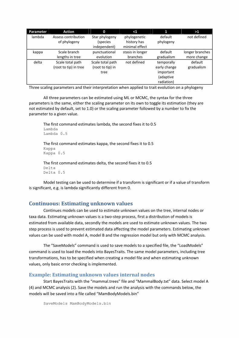
Parameter Action 0 <1 1 >1

lambda Assess contribution of phylogeny

Star phylogeny(species

independent)

phylogenetic history has

minimal effect

default phylogeny

not defined

kappa Scale branch lengths in tree

punctuationalevolution

stasis in longer branches

default gradualism

longer branchesmore change

delta Scale total path (root to tip) in tree

Scale total path(root to tip) in

tree

not defined temporally early change important (adaptive radiation)

defaultgradualism

Three scaling parameters and their interpretation when applied to trait evolution on a phylogeny

All three parameters can be estimated using ML or MCMC, the syntax for the three parameters is the same, either the scaling parameter on its own to toggle its estimation (they are not estimated by default, set to 1.0) or the scaling parameter followed by a number to fix the parameter to a given value.

The first command estimates lambda, the second fixes it to 0.5 Lambda Lambda 0.5

The first command estimates kappa, the second fixes it to 0.5 Kappa Kappa 0.5

The first command estimates delta, the second fixes it to 0.5 Delta Delta 0.5

Model testing can be used to determine if a transform is significant or if a value of transform is significant, e.g. is lambda significantly different from 0.

Continuous:Estimatingunknownvalues Continues models can be used to estimate unknown values on the tree, internal nodes or

taxa data. Estimating unknown values is a two‐step process, first a distribution of models is

estimated from available data, secondly the models are used to estimate unknown values. The two

step process is used to prevent estimated data affecting the model parameters. Estimating unknown

values can be used with model A, model B and the regression model but only with MCMC analysis.

The “SaveModels” command is used to save models to a specified file, the “LoadModels”

command is used to load the models into BayesTraits. The same model parameters, including tree

transformations, has to be specified when creating a model file and when estimating unknown

values, only basic error checking is implemented.

Example:Estimatingunknownvaluesinternalnodes Start BayesTraits with the “mammal.trees” file and “MammalBody.txt” data. Select model A

(4) and MCMC analysis (2). Save the models and run the analysis with the commands below, the

models will be saved into a file called “MamBodyModels.bin”

SaveModels MamBodyModels.bin

Run

Once the program has finished a file called “MamBodyModels.bin” will be created.

To estimate data, start BayesTraits with the same tree and data files, select model A (4) and MCMC analysis (2). The AddMRCA command is used to estimate internal node values, it takes a node label used to identify the node in the output and a list of taxa which define the node. The commands below load the model file, reconstruct a node called “Node‐01” defined by five taxa, reconstruct a node called “Node‐02” defined by four taxa, and run the analysis. LoadModels MamBodyModels.bin AddMRCA Node-01 Whale Hippo Llama Ruminant Pig

AddMRCA Node-02 Mouse Rat Hystricid Caviomorph Run

The output header will contain Header Output





Model No Current model number from the model file

Alpha Trait 1 Phylogenetic mean

Var Trait 1 Brownian motion variance

Est Node‐02 ‐ 1 Estimated values for Node‐02 trait 1

Est Node‐01 ‐ 1 Estimated values for Node‐01 trait 1

Example:Estimatingunknownvaluesfortips Data for taxa can be estimated, as well as internal nodes. A data file “MammalBrainBodyNoTapir.txt” has been created with the data for tapir set to missing ‘‐‘. Run BayesTraits with the “Mammal.trees” tree file and “MammalBrainBodyNoTapir.txt” data file. Select the regression model (6) and MCMC analysis (2). Use the command below to save the models and run the analysis SaveModels MamRegModels.bin Run

A data file “MammalBrainBodyPredTapir.txt” which contains the tapir body size but with the brain size set to “?”, a question mark in the data is used to indicate the value should be estimated. Run an analysis using the “Mammal.trees” tree file and “MammalBrainBodyPredTapir.txt” data file. Select the regression model (6) and MCMC analysis (2). Use the command below to load the models and run the analysis LoadModels MamRegModels.bin Run

The output will contain a “Est Tapir – Dep” column, with the predicted tapir brain size.

Independentcontrast BayesTraits implements a independent contrast models which can be estimated using

MCMC or ML. Start BayesTraits with the tree file “Mammal.trees” and data file

“MammalBrainBody.txt”. Select Independent contrast (7) and MCMC (2) and run the analysis.

The independent contrast model assumes sites are independent. The output will contain

Header Output





Alpha 1 Phylogenetic mean of the first trait

Alpha 2 Phylogenetic mean of the second trait

Sigma 1 Brownian motion variance for the first trait

Sigma 2 Brownian motion variance for the second trait

Variableratesmodel The variable rates model allows the rate of change to vary threw time and identifies areas of

the tree where the rate of evolution differed significantly, for an in‐depth description see (ref). The

variable rates model uses RJ MCMC to identify areas of the tree in which the rate of evolution varies

significantly. The model only works with a single tree and requires MCMC analysis. A tree

(Marsupials.trees)of roughly 250 Marsupials and there body sizes (Marsupials.txt) is included. Start

BayesTraits with the tree and data file, select Independent contrast (7) and MCMC (2), run the

variable rates analysis with the commands below.

VarRates Run

The log file will contain

Header Output





Alpha 1 Phylogenetic mean of the first trait

Sigma 1 Brownian motion variance for the first trait

No VarRates Number of areas of the tree with variables rates

Other data files are created, “Marsupials.txt.PP.trees” contains the trees modified by the

variables rates, areas which are stretched have an increased rate of change, areas which are

shrunken have a decreased rate. The file “Marsupials.txt.PP.txt” contrails a detailed description of

the changes, the format of the file is, line 1, number of taxa, followed by a unique taxa ID and taxa

name. The second part is the number of internal nodes, followed by a list of internal nodes

consisting of a unique node ID, branch length (‐1 for root), number of taxa which define the node

and the list of taxa ID. The third section details the results of the chain, the columns are

Header Output

It Iteration of the chain

Lh Likelihood of the chain

Lh + Prior Likelihood + prior

No Pram Number of change to rate of the tree

Alpha Estimated phylogenetic mean

Sigma Brownian motion

Alpha Scale Scale of the prior (unchanging, for diagnostics only)

For each change of rate of the tree (No Param) there is

Header Output

Node ID The node if the change is on

Scale The scale of the change

Crate It The iteration the change was created on

Node / Branch If the change is a node or branch scale

The .PP.txt file is designed to be computer read, post processing tools will shortly be made

available to extract useful information from the file.

CommandList Command: // Purpose: Add a comment. Shortcut: # Parameters: None Example: # This is a comment.

Command: AddMRCA Purpose: To reconstruct an internal node using the most recent common ancestor approach Shortcut: MRCA Parameters: A node name and a list of taxa names or number that define a node to reconstruct. Example: AddMRCA Node1 Taxa1 Taxa2 Taxa3 MRCA Node1 1 2 3 4 Command: AddNode Purpose: To reconstruct an internal node. Shortcut: AddN Parameters: A node name and a list of taxa names or number that define a node to reconstruct. Example: AddNode Node1 Taxa1 Taxa2 Taxa3 AddN Node1 1 2 3 4

Command: AlphaZero Purpose: Sets the intercept to zero Shortcut: AZ Parameters: None Example: AlphaZero

Command: BurnIn

Purpose: To set the number of iterations to burn the MCMC chain in for, use ‐1 for an infinite chain.

Shortcut: BI Parameters: An integer Example: BurnIn 50000 BI ‐1

Command: CapRJRates Purpose: Cap the maximum number of reverse jump rates to use Shortcut: Cap Parameters: An integer, >0 Example: CapRJRates 2

Cap 1 Command: CoVarion Purpose: Turn on/off the convarion model Shortcut: CV Parameters: None Example: CoVarion CV Command: DataDev Purpose: Set the deviation parameter to used when perturbing estimated data. This value

should be automatically set, modifying the value is not recommended. Shortcut: DD Parameters: A number, >0 Example: DataDev 2.0 DD 01 Command: Delta Purpose: Estimate delta or set it to a fixed value Shortcut: DL Parameters: None to estimate delta, or a number to fix it to a value Example: Delta Delta 0.5 Command: EqualTrees Purpose: Force the chain to spend an equal amount of time on each tree in the sample. This

results in a separate posterior distribution pre tree. Shortcut: EQT Parameters: Number of iterations to burn each tree in for. Example: EqualTrees 20000

Command: EvenRoot Purpose: Set midpoint rooting for the sample. Shortcut: ER Parameters: None Example: EvenRoot

Command: Exit Purpose: Exit BayesTraits without running the analysis

Shortcut: Quit Parameters: None Example: Exit

Command: Fossil Purpose: Fix an internal node to a specific value Shortcut: FO Parameters: A name, the value to fossilise the node in and a list of taxa which define the node.

See the fixing node values section above for more information. Example: Fossil AnsNode D 12 13 14 15 16 17 Fossil Base 2 Hylobates_gabriellae Hylobates_leucogenys Hylobates_concolor Command: Gamma Purpose: Estimate or fix gamma rate heterogeneity. Shortcut: GA Parameters: The number of gamma categories and an option value to fix the parameter Example: Gamma 4 Gamma 4 0.5

Command: Help Purpose: Print a list of commands, not all are valid / working Shortcut: he Parameters: none Example: Help

Command: HyperPrior Purpose: Set a hyper prior on a parameter Shortcut: HP Parameters: A parameter name, a distribution name, and range to draw each parameter from Example: HyperPrior q01 exp 0 100 HP q10 gamma 0 100 0 100 Command: HyperPriorAll Purpose: Set all priors to a common hyper prior Shortcut: HPAll Parameters: A distribution name and range to draw each parameter from Example: HyperPriorAll Beta 0 100 0 50 HPAll Exp 0 200

Command: Info Purpose: Print current options Shortcut: in Parameters: None Example: Info

Command: Iterations Purpose: Set the number of iterations to run the chain for Shortcut: IT Parameters: The number of iterations to run the chain for, or ‐1 for an infinite chain, use Ctrl+C

for termination. Example: Iterations 1000000 IT ‐1

Command: Kappa Purpose: Set the kappa scaling parameter Shortcut: KA Parameters: None to estimate kappa, or a number to fix it to value Example: Kappa KA 0.1 Command: Lambda Purpose: Set the lambda scaling parameter Shortcut: LA Parameters: None to estimate lambda, or a number to fix it to value Example: Lambda LA 0.8

Command: LoadModels Purpose: To load models from a model file, see SaveModels Shortcut: LM Parameters: A model file name Example: LoadModels ModelFile.bin

Command: MLTries Purpose: Set the number of times to find the maximum likelihood values, higher values are

more consistent but take longer to run Shortcut: MLT Parameters: Number of maximum likelihood tries, default 10. Example: MLTries 35 MLT 100 Command: Pis Purpose: Set the base frequencies Shortcut: Pi Parameters: Set the base frequencies estimates, est, emp, uni and none est for estimate

frequencies, emp for empirical, uni for uniform and none not to use any (all set to 1).

Example: Pis emp Pis uni Pis est Pis none Command: Prior Purpose: Set the prior for a parameter Shortcut: pr Parameters: a parameter, a distribution type and parameters, distributions include, beta, gamma,

uniform and exp Example: Prior alpha1 exp 10 Prior q01 gamma 10 5 Prior q10 Beta 2.5 1 Prior q34 Uniform 0 1 Command: PriorAll Purpose: Set the prior for all parameters Shortcut: PA

Parameters: A distribution type and parameters, see prior command Example: PriorAll Exp 10 PriorAll Beta 1 7 Command: PriorCats Purpose: Specify the number of categories to divide the prior into, default 100. Shortcut: PCat Parameters: An integer > 1, Example: PriorCats 200 PCat 50 Command: RateDev Purpose: Sets the rate deviation parameter, effecting acceptance rate. The new version

automatically finds a good acceptance rate. Setting it manually is an advanced option and should be avoided.

Shortcut: RD Parameters: None to automatically estimate the parameter, an value to set all parameters to the

same value, a parameter name and value to set a specific parameter to a value, only for continuous models.

Example: RateDev RateDev 12.5 RateDev alpha‐1 0.3 Command: Restrict Purpose: Restrict a parameter or parameters to another parameter of a fixed value. Shortcut: Res Parameters: A list of parameter to restrict, a parameter or fixed value to restrict to. Example: Restrict alpha1 beta1

Restrict alpha1 beta1 alpha2 beta2 Restrict beta1 beta2 1.5

Command: RestrictAll Purpose: Restrict all parameter to a parameter or fixed value Shortcut: ResAll Parameters: A parameter or fixed value Example: RestrictAll alpha1 ResAll 0.75 Command: RevJump Purpose: Set a reverse jump analysis Shortcut: RJ Parameters: A prior and prior parameter Example: RevJump exp 10 RevJump Gamma 4 20 RJ Beta 5.0 2.5 Command: RevJumpHP Purpose: Set a reverse jump analysis with a hyper prior Shortcut: RJHP Parameters: A hyper prior Example: RevJumpHP exp 0 100 RevJumpHP gamma 0 100 0 50

Command: Run Purpose: Run the analysis Shortcut: RU Parameters: None Example: Run

Command: Sample Purpose: Set the sample frequency Shortcut: SA Parameters: An integer > 0 Example: Sample 1000 Sample 250 Command: SaveModels Purpose: Save the models to a file Shortcut: SM Parameters: A file name to save the models to. Example: SaveModels ModelFile.bin SM ModelFile.bin Command: SaveTrees Purpose: Save the sample of trees before analysis Shortcut: ST Parameters: A filename to save the trees to Example: SaveTrees STrees.trees

Command: Seed Purpose: Set the random seed Shortcut: se Parameters: An integer, > 0, to seed the random number from Example: Seed 39362

Se 483 Command: Symmetrical Purpose: Make restrictions to create a symmetrical matrix Shortcut: SYM Parameters: none Example: Symmetrical SYM

Command: TaxaInfo Purpose: Show taxa names and numbers Shortcut: TI Parameters: None Example: TaxaInfo Command: TestCorrel Purpose: To set the correlation between traits to zero, used for model testing. Shortcut: TC Parameters: None Example: TestCorrel

Command: UnRestrict Purpose: Remove a parameter restriction Shortcut: UNRes Parameters: A parameter to un restrict Example: UnRestrict q01

Command: UnRestrictAll Purpose: Remove all restrictions Shortcut: UnResAll Parameters: none Example: none

Command: VarRates Purpose: Use the variable rates model Shortcut: VR Parameters: None Example: VarRates

Commonproblem/FrequentlyAskedQuestions

1) Problems running the program Q) Double clicking on the program does not work.

A) BayesTraits is run from the command line and not by double clicking on it. See “Running BayesTraits” section.

2) Common tree and data errors

A) Tree must be in nexus format with a valid translate block. Use the example files as a template.

B) Tree descriptions must have number and not taxa name in them. C) Trees must be rooted. D) Trees and data must be encoded using ASCII format not Unicode E) The error “Could not load data for taxa X”, this error is caused by a taxa being specified

in the tree file but not in the data file. Check spelling and taxa numbers F) The error “Tree file does not have a valid nexus tag.” Is because a nexus tag is not found

in the tree file. Possible causes are specifying the data file before the tree file.

3) Error message “Memory allocation error in file …”, the two main causes of memory allocation errors are running out of memory, this can be due to too many trees in the tree file or complex memory intensive models. Check the programs memory usage, if you have a 64 bit OS use the 64 bit version of the program. Try running the program with a smaller number of trees and simpler models. The second cause of the error is due to programming errors, if you believe this is the case, please send along the tree file, data file and set of command used. 4) Chain is not mixing between trees. This problem can be caused when one tree’s likelihood is significantly better than other trees in the sample. Trees are sample in proportion to their likelihood, if one is much better than the rest it will be sample much more often. This can be a particular problem with a large number of trees when the topology is poorly supported, a chance combination create a much better likelihood preventing the chain from mixing. To test if this is the problem run the sample using ML, this will determine if the tree which the chain gets stuck on has the best likelihood. Two options are available, the first is to remove the tree from the sample if you believe it is anomalous for some reason. The second is to use the Equal Tree command to force the chain to spend an equal amount of time on each tree. The equal tree command will produce a separate posterior sample of rates, parameters and ancestral states per tree, instead of a single set integrated over the sample of trees.

References

bayestraits v2 (beta, unfinished) july 2013beta).pdf · 2014-06-02 · bayestraits v2 (beta,...

Documents