bearing fault diagnosis using multiclass support vector...

International Journal of Mechanical & Mechatronics Engineering IJMME-IJENS Vol:15 No:01 1

150401-9292-IJMME-IJENS © February 2015 IJENS I J E N S

Bearing Fault Diagnosis using Multiclass Support

Vector Machine with efficient Feature Selection

Methods C.Rajeswari

1, B.Sathiyabhama

2, S.Devendiran

3& K.Manivannan

4

1 Research Scholar, Faculty: Information and Communication Engineering, Anna University, Chennai, India

[email protected] 2Department of Computer Science and Engineering, Sona College of Technology, Salem, Tamil Nadu, India

[email protected] 3,4

School of Mechanical and Building Sciences ,VIT University, Vellore, Tamil Nadu, India

[email protected]

[email protected]

Abstract--- Fault diagnosis in bearings has been the subject

of intensive research as bearings are critical component in many-

rotating machinery applications and an unexpected failure of the

bearing may cause substantial economic losses. Vibration analy-

sis has been used as a predictive maintenance procedure and as a

support for machinery maintenance decisions. In this study, we

used Multiclass Support Vector Machines (MSVM) for classifica-

tion task. SVM is a powerful classification tool that is becoming

increasingly popular in various machine-learning applications. In

data pre-processing step advance signal processing methods such

as wavelet transform is used to extract the features which reveals

the characteristics of the actual conditions of the bearing. To

reduce the dimensionality of the feature SVM–Recursive Feature

Elimination (SVM-RFE),Wrapper subset method, ReliefF meth-

od and Principle component analysis (PCA). Moreover, investiga-

tion is done performance of MSVM with mentioned different

feature selection strategies as well as MSVM alone on basis of

classification accuracy. To validate the proposed methodology,

four kinds of running states are simulated with artificially creat-

ed faults in bearing that is accommodated in the test rig. By com-

paring classification accuracy along with computation timing the

best scheme is selected for diagnostic prediction.

Index Term-- Test rig, fault diagnosis, wavelet, SVM–Recursive

Feature Elimination, Wrapper subset method, ReliefF method

and Principle component analysis(PCA)

I. INTRODUCTION

The performance of bearing is highly influential on perfor-

mance of any rotating machine and it is consider as a heart of

rotating machinery. Monitoring the dynamic behaviour and

health condition of significant machine element bearing is in

evitable and thereby provide an alarm and instructions for

preventive maintenance by means of advanced sensors, data

collection systems, data storage/transfer capabilities and data

analytic tools developed for such purpose. Fault prediction is

one of the important undertakings during the maintenance

work. Vibration signal based bearing fault diagnosing method

is prominently used over the past two decades [1,2]. When a

fault occurs in a bearing, periodic impulses appear in the time

domain of the vibration signal, while the corresponding bear-

ing characteristic frequencies (BCFs) and their harmonics

emerge in the frequency domain [3]. However, in the early it

get suppressed by severe noise and higher-level vibrations.

Consequently an effective signal processing method is of ut-

most importance for the extraction of damage sensitive fea-

tures during the condition monitoring of bearings. Generally,

the failure of a mechanical system is always accompanied with

the changes of vibration characteristics from linear or weak

nonlinear to strong nonlinear dynamics [4,5].Until now, in the

field of bearing fault detection, a variety of approaches and

time–frequency signal processing tools have been utilized.

Wavelet transform (WT) has been widely used as a de-noising

tool as well as for feature extraction in rotating machinery

diagnostics [6].The Wavelet Transform (WT) provides power-

ful multi-resolution analysis in both time and frequency

domains. The fault diagnosis of rolling bearing in early stage

using wavelet packet transform and empirical mode decompo-

sition were combined and extracted features are given as input

to neural network after analysing the shortcomings of current

feature extraction and fault diagnosis technologies[7].In past

decades, sometime-frequency analysis methods, including

short time Fourier transform (STFT) [8], Wigner–Ville distri-

bution (WVD) [9,10], and local mean decomposition(LMD)

[11], have been formulated to probe non-stationary data and

applied to feature extraction of defective rotary machinery.

However, each of these methods leaves something to be de-

sired and some even perform badly in analysing non-

stationary and nonlinear data [12].

The early stage rolling failure diagnostic methods include the

use of hearing, shock pulse and frequency demodulation tech-

nologies with lower industry standard accuracy and efficiency

in diagnosis .With the continuous development of diagnostic

techniques, artificial intelligence, such as expert system, artifi-

cial neural network (ANN), fuzzy logic, Roughset, genetic

algorithm have been widely used in machine fault diagnosis

[13-16] based on the empirical risk minimization principles.

Unfortunately, because of the bottleneck of knowledge acqui-

sition, the application of expert system is limited. Also, for the

complexity of machinery and knowing little of the fault mech-

anism, the diagnosis methods based on neural network and

soft-computing technology need to be studied further to im-

prove the diagnosis performance, such as increasing diagnosis

accuracy and decreasing running time, etc. In intelligent fault

diagnosis method, statistical characteristics were calculated



after signal processing and it hasvast number of features with-

in variety domains poses challenges to data mining. In order to

achieve successful classification process in terms and predic-

tion accuracy, feature selection is consider as essential. Fea-

ture selection methods such as principal component analysis

(PCA) [7] and Genetic algorithm (GA) [8] and J48 algorithm

[9] are widely used to decrease dimensions of features proved

for its meaningful diagnostics process. In the present work,

most suitable signal processing technique based on sub-band

coding and known for its fast computation among the wavelet

family called discrete wavelet decomposition is used for ex-

tracting wavelet coefficients and statistical features are ex-

tracted for different levels of decomposition and fed into

MSVM for classification process. For comparison of the pre-

diction accuracy C4.5 is introduced and applied to bearing

fault diagnosis .To reduce the response time of classification

process the most significant feature selection methods were

introduced, analysed and discussed about the importance of

the feature selection method.

In Section 1 we briefly reviewed the works which are strictly

connected to the subject of this paper. In Section 2 contains

theoretical background of wavelet transform, statistical fea-

tures and feature reduction methods were discussed. In Sec-

tion 3 Experimental setup and experimental procedure is pre-

sented. In Section 4 Analysis of simulated data according to

the presented procedure is presented. In Section 5 the results

for the same is presented and Last section contains conclu-

sions. The methodology of the present work is illustrated in

the Fig.1

Fig. 1. Proposed experimental methodology

II. THEORETICAL BACKGROUND OF FEATURE EXTRACTION AND

FEATURE SELECTION

A. Wavelet transform

The aim of signal processing is to find the health condition of

the rotating component using vibration signal. Recently, wave-

let transform (WT), which is capable of providing both the

time- domain and frequency-domain information simultane-

ously, has been successfully used in non-stationary vibration

signal processing and fault diagnosis [20]. In this present work

wavelet transform is used in feature extraction .The two type

of wavelet Continuous wavelet transform(CWT) and Discrete

wavelet transform (DWT) are discussed below. A series of

oscillating functions with different frequencies such as win-

dow function for scanning, x(t) for translating the

signal are used in wavelet transform, where α is the oscillat-

ing frequency changing parameter and β is the translation pa-

rameter. A high frequency resolution is obtained when the

frequency is low at low time resolution and a low frequency

resolution is obtained when the frequency is at low time reso-

lution.

The function with the parameter α and β with mother wavelet

is given as:

(1)

If all signals x(t) satisfy the condition then,

(2)

that gives x(t) decays to zero.

The wavelet transform, CWT (α ,β ) , of a time signal x(t) can

be given as

(3)

Where an analyzing wavelet is 𝛹 and will be the

complex conjugate of 𝛹 . For analyzing the different wave-

let, real and complex valued function can be used.A lot of

redundant data is created by calculating the wavelet coeffi-

cient at possible scale. Thus the analysis can be made suffi-

cient and accurate by giving the limit of choice of α and β to

discrete numbers.

By selecting the fixed values and ,

we get the DWT

(4)

If α and β are replaced by and , then the DWT is de-

rived as

(5)

Thus the high and low frequency signal is obtained from the

original signals by decomposition process. The daubechies

wavelet transform is used in this process because of its less



process consuming time. As well it is in the family of orthog-

onal wavelet. This is a type of multi resolution analysis and

mostly used for solving a wide range of problems with large

dataset. The scaling function of daubechies wavelet is given as

db1-db15. It is noted that the highest level of efficiency is tak-

en for the analysis by the Daubechies wavelet.

B. Feature extraction

The bearing fault diagnostic task is actually a problem of

pattern classification and pattern recognition, of which the

crucial step is feature extraction. In the machinery fault diag-

nosis field, features are often extracted in time domain and

frequency domain. But In this paper, we extract features from

wavelet decomposition data. There are many feature parame-

ters are available and the features that taken for this proposed

work is listed in Table I.

TABLE I

STATISTICAL FEATURE

C. Support Vector Machine – Recursive Feature Ex-

traction (SVM-RFE)

SVM-RFE is an iterative process that is used to eliminate

redundant features and yield better subsets. SVM-RFE uses

weight magnitude as the ranking criterion. This process

involves three steps; training the SVM on the given training

data set, ranking the features based on their weights, and

eliminating the feature with the lowest weights. The inputs

given for the SVM-RFE process are the training samples,

(6)

and class labels, (7)

The subset of the persisting features are given as

(8)

From the given training data set, we build the SVM model,

and is given as

(9)

after training the SVM model the weight vector of dimen-

sion length is computed and is given as

(10)

the ranking criteria is computed for the weighted vectors,

the persisting feature ranked list is updated from which

the feature with smallest ranking criterion is eliminated.

The accuracy of the classifier is evaluated by using 10 fold

cross validation. Ranker is used as the search method. The

ranker search method uses information gain measure to

select the relevant attributes. More details about SVM –

RFE can be found in [21].

D. Wrapper Subset Evaluation:

This method calculates the feasible attribute subsets using

target learning algorithm. The wrapper method uses Greedy

stepwise method as the search method. Survey shows that

wrapper method provides better results than filter method

because of the interaction between the search and the learn-

ing process. But this performance is achieved at the expense

of computational cost incurred during invoking the learning

algorithm for every feature subset. The greedy stepwise

method ranks the attributes either in the stepwise forward or

backward selection process. 10 fold cross validation is used

to estimate the accuracy of a classifier. Cross validation is

repeated as long as the standard deviation is greater than the

Statistical feature Equation

Definition

Kurtosis 4

1

1( )

n

kur

i

k k t kn

Fourth central moment of „X‟,

divided by fourth power of its

standard deviation.

Skewness

3

1

1( )

n

skew

i

k k t kn

Third central moment of the

value, divided by the cube of

its standard deviation.

Variance 2

var

1

1( )

n

i

k k t kn

Measures how far a set of

numbers is spread out

Standard deviation 2

1

1( )

1

n

Sd i

i

k kn

Square root of an unbiased

estimator of the variance of

the population

Root mean square

2

1

1 n

rms

i

k kn

Root of sum of squared values



mean accuracy or until 10 repetitions are reached. More

details about wrapper subset can be found in [22].

E. ReliefF Attribute Evaluation :

ReliefF (RF) method evaluates the worth of an attribute by

repeatedly sampling an instance and considering the value

of the given attribute for the nearest instance of the same

and different class. It can operate on both discrete and con-

tinuous class data. The RF is not limited to two class prob-

lems and is more robust and can deal with incomplete and

noisy data. RF selection process is based on ranking the

features with higher weight in order to decrease the chance

of selecting features with lower weight. For more infor-

mation about ReliefF refer [23,24].

F. Principal Component Analysis (PCA)

PCA is a statistical technique that is used to reduce the di-

mensionality of the data. In order to reduce the number of

features and dimensions of the features without affecting

the usefulness of the features, feature reduction method is

used. Among all the feature reduction techniques PCA is

the only unsupervised technique that is it does not bother

about the values of the class labels. From the given set of n

dimension feature vectors (t=1, 2, 3……, m), generally

n<m, the mean is calculated as,

(11)

then by using the formula in (7), the covariance matrix of

feature vector is found

(12)

by solving the eigen value problem of covariance matrix C,

The principal components (PCs) is obtained

(13)

Where 𝜆 (i= 1, 2,…, n) are the eigen values and they are

sorted in descending order. (i=1, 2,...n) are the corre-

sponding eigenvectors. For the raw feature vectors with

low-dimensional ones, compute the first k eigenvectors (k ≤

n) which correspond to the biggest k eigen values. In order

to select the number k, a threshold 𝜃 is introduced to de-

note the biggest k eigenvectors.

(14)

Given the precision parameter 𝜃, the number of eigenvec-

tors k can be decided.

For any given dataset, the eigen vectors are

….. (15)

once the matrix V is determined, the low-dimensional fea-

ture vectors, named principle component (PC), of raw ones

are obtained as follows,

(16)

The Principal Component‟s (PCs) of PCA have three prop-

erties according to [25]

1) They are uncorrelated; 2) they have sequentially maxi-

mum variances; 3) the mean-squared approximation error in

the representation of the original vectors by the first several

PCs is minimal.

III. EXPERIMENTAL SETUP AND EXPERI-

MENTALPROCEDURE

The proposed methodology is verified by performing tests

on the designed experimental setup. The experimental set-

up shown in Fig.2 comprises of components such as varia-

ble frequency drive (VFD), three phase 0.5 hp AC motor,

bearing, belt drive, gear box and brake drum dynamometer

with scale. This experiment utilizes a standard deep groove

ball bearing (No. 6005). Measurements of the vibration

acceleration signals are captured by a tri-axial type accel-

erometer that is fixed over the bearing block. A 24 bit data

acquisition system was used and the signals were collected

at a sampling frequency of 12800 Hz. The bearing was

maintained at a constant rotating speed of 1700 r/min. The

brake drum dynamometer applied a constant load and the

speed was monitored by a tachometer. Fig.2 also depicts

normal, outer race, inner race and ball fault (1mm crack

depth) conditions were formed using the EDM process.

Initially the vibration data is collected for each bearing

condition for around 30 seconds in the sampling rate of

12800Hz and it is separated into many data sets for classifi-

cation purpose. Each sample set contains 6000 data points.

In general analysis of the signal is done to find out various

conditions of bearing component using time domain and

frequency domain by varying amplitudes. Time domain

plots are illustrated in Fig.3(a). One of the most basic

approach for bearing conditioning monitoring is Frequency

analysis.



Fig. 2. Bearing test rig (experimental set up) and induced bearing faults

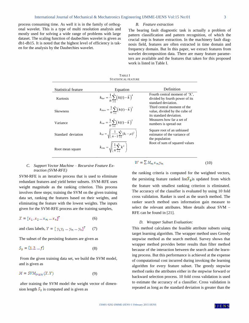
Fast Fourier transform (FFT), is used to transform the time

series data to frequency domain, where the signal is used to

deduce the sine and cosine waves from the sample. In practice,

analysing those characteristic frequencies such as BPFO- Ball

Pass Frequency Outer Race, BPFI- Ball Pass Frequency Inner

Race, FTF- Fundamental Train Frequency and BSF- Ball Spin

Frequency and measuring the amplitude variations in the

characteristic frequency and its side bands as well the harmon-

ics of those frequencies will provide information regarding the

health of the bearing. Even though the bearing conditions are

difficult to be differentiated by their FFT spectral shown in

Fig.3 (b).

Fig. 3(a). Time domain signals of various states of bearing(X axis–data points, Y axis-Amplitude in „g‟)



Fig. 3(b). Frequency spectrum of various states of bearing (X axis–Frequency, Y axis-Amplitude in „g‟)

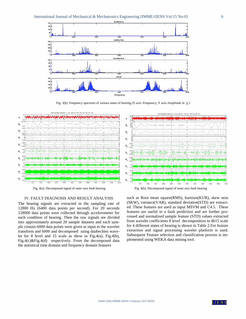
IV. FAULT DIAGNOSIS AND RESULT ANALYSIS

The bearing signals are extracted in the sampling rate of

12800 Hz (6400 data points per second). For 20 seconds

128000 data points were collected through accelerometer for

each condition of bearing. Then the raw signals are divided

into approximately around 20 sample datasets and each sam-

ple contain 6000 data points were given as input to the wavelet

transform and 6000 and decomposed using daubechies wave-

let for 8 level and 15 scale as show in Fig.4(a), Fig.4(b),

Fig.4(c)&Fig.4(d) respectively. From the decomposed data

the statistical time domain and frequency domain features

such as Root mean square(RMS), kurtosis(KUR), skew ness

(SKW), variance(VAR), standard deviation(STD) are extract-

ed. These features are used as input MSVM and C4.5. These

features are useful in a fault prediction and are further pro-

cessed and normalized sample feature (STD) values extracted

from wavelet coefficients 8 level decomposition in db15 scale

for 4 different states of bearing is shown in Table 2.For feature

extraction and signal processing wavelet platform is used.

Subsequent Feature selection and classification process is im-

plemented using WEKA data mining tool.

Fig. 4(a). Decomposed signal of outer race fault bearing Fig. 4(b). Decomposed signal of inner race fault bearing



Two classifier learners were employed for the classification of

the data, Weka incorporated C4.5 (J48) and MSVM (SMO)

and is used and for theoretical background of C4.5 refer [25]

and For more information on the SMO algorithm, see [26].The

Waikato Environment for Knowledge Analysis (Weka) is a

comprehensive suite of Java class libraries that implement

many state-of-the-art machine learning and data mining algo-

rithms. Tools are provided for pre-processing data, feeding it

into a variety of learning schemes, and analysing the resulting

classifiers and their performance [27-28]. The experiment was

carried out with and without feature selection schemes. The

tool is used to perform benchmark experiment.

TABLE II SCHEMATIC REPRESENTATION OF STATISTICAL FEATURES

As per the diagnosis methodology, features are selected using

4 different feature selection methods SVM–Recursive Feature

Elimination , Wrapper subset method, ReliefF method and

Principle component analysis (PCA) and It is compared (Table

4) based on the execution or elapsed time period shown in

Fig.5. Among the selection methods SVM–Recursive Feature

Elimination taken a less execution timing compare to all other

methods but when compare to prediction accuracy

it is not on the top of the list (shown in Table 5) along with

both classifiers MSVM and C4.5 .The prediction results for

single (sample)dataset are clearly depicted in the Table 5 , it

contains number of features selected for each scheme, each

bearing element individual accuracy, average accuracy and

mean absolute error . Among all the schemes MSVM-S3 gives

the best result of 95% of classification accuracy and less

0.0129 mean absolute error even though with less number of

features(14 Nos.)

Feature d1 d2 d3 d4 d5 d6 d7 d8

RMS F1 F2 F3 F4 F5 F6 F7 F8

KUR F9 F10 F11 F12 F13 F14 F15 F16

SKW F17 F18 F19 F20 F21 F22 F23 F24

VAR F25 F26 F27 F28 F29 F30 F31 F32

STD F33 F34 F35 F36 F37 F38 F39 F40

Fig. 4(c). Decomposed signal of ball fault bearing Fig. 4(d). Decomposed signal of normal bearing



TABLE III

SAMPLE STATISTICAL FEATURES (NORMALIZED) VALUES OF STD EXTRACTED FROM

WAVELET COEFFICIENTS 8 LEVEL DECOMPOSITION IN DB15 SCALE FOR 4 DIFFERENT STATES OF BEARING.

Bearing fault diagnosis results are also evaluated and com-

pared based on standard parameters such as classification ac-

curacy, sensitivity and specificity for various classifiers are

proposed in this work and it is depicted in Table 6.It is inter-

esting to note that an increase in classification accuracy is

recorded for the proposed feature reduction methods, with

respect to the unreduced data in most of the cases. Also, when

comparing classification results, the feature reduction methods

have the more or less same classification accuracy values

which are recorded in most of the cases.

They are demonstrated in Fig.6 & Fig.7. Test carried out for

different data sets and classification accuracy is depicted in

Table VII and it shows the MSVM-S3 scheme comprise of

wrapper feature selection method and support vector machine

classifier with 14 selected features gives the maximum accu-

racy of 96% overall for all four conditions of bearings with

mean absolute error of 0.0137. On an average compare to

other schemes MSVM-S3 gives better result.

TABLE IV

ELAPSED TIME FOR DIFFERENT FEATURE SELECTION METHODS IN SECONDS

States d1 d2 d3 d4 d5 d6 d7 d8

Normal 1 0.283462 0.053757 0 0.027785 0.002573 0.017349 0.012132

Normal 0.673831 0.103484 0.931932 1 0.759407 0.8299 0.92486 0.955869

Normal 0.801204 0.007884 0.903114 0.956812 0.735277 0.748216 0.937741 0.985658

. . . . . . . . .

. . . . . . . . .

Ball fault 0.073152 0.933981 0.083051 0.051354 0.120508 0.015602 0.006983 0.000759

Ball fault 0.098997 0.926975 0.097925 0.047301 0.103161 0.013037 0.000451 0.000175

Ball fault 0.390674 0.707986 0.138631 0.041442 0.070923 0.015776 0.001171 0

Sl.No Feature selection

scheme

Data set

1 2 3 4 5 6 7 8 9 10

1 No feature selection 0.000 0.000 0.000 0.000 0.000 0.000 0.000 0.000 0.000 0.000

2 SVM-RFE 0.093 0.082 0.073 0.089 0.095 0.087 0.090 0.079 0.073 0.078

3 Wrapper subset 1.762 1.521 1.020 1.890 1.678 1.569 1.700 1.432 1.178 1.281

4 ReliefF 0.385 0.207 0.359 0.289 0.217 0.223 0.323 0.345 0.268 0.290

5 PCA 2.261 2.011 1.721 2.523 2.610 1.890 2.200 2.412 1.891 1.359



Fig. 5. Different data set Vs Execution timing of feature selection methods

Fig. 6. Classification accuracy of MSVM with different feature reduction methods for different datasets

Fig. 7. Classification accuracy of C4.5 with different feature reduction methods for different datasets

Table Table.5. Performance comparison of classifiers with and without feature selection



TABLE V

PREDICTION RESULTS OF DIFFERENT SCHEMES OF CLASSIFIERS

TABLE VI RESULTS OF DIFFERENT PREDICTION PARAMETERS FOR SINGLE DATA SET

Classi-

fier

Feature

selection

method

Scheme

name

No. of

selected

features

Feature description

Prediction accuracy of test data in

(%) Average

Accuracy

on testing

data (%)

Mean

absolute

error Normal

Inner

ner-

race

fault

Outer

race

fault

Ball

fault

C4.5

No feature

selection

C4.5-S1 All(40) F1-F40 80 83 81 80 81.00 0.1082

SVM-

RFE

C4.5-S2 18

F1,F7,F13,F18,F20,F21,F23,F2

4,F25,F27,F28,F29,F31,F34,F3

5, F37,F38,F40.

93 86 88 90 89.25 0.1954

Wrapper C4.5-S3

14

F1,F2,F4,F5,F10,F13,F17,

F21,F25,F28,F29,F30,F33,

F36

95 97 94 94 95.00 0.0129

ReliefF C4.5-S4

20

F1,F2,F5,F7,F8,F11,F13,F15,F

16,F17,F18,F21,F24,F27,F28,F

29, F31,F34,F36,F37.

95 96 90 87 92.00 0.0157

PCA C4.5-S5

11

F1,F2,F4,F5,F8,F9,F10,F13,F1

7,F21,F25,F27,F28,F29,F30,F3

3, F36.

92 90 93 94 92.25 0.0198

MSVM

No feature

selection MSVM-S1 All(40) F1-F40 85 87 83 80 83.75 0.2942

SVM-

RFE

MSVM-S2 18

F1,F7,F13,F18,F20,F21,F23,F2

4,F25,F27,F28,F29,F31,F34,F3

5, F37,F38,F40.

90 89 93 91 90.75 0.1848

Wrapper MSVM-S3

14 F1,F2,F4,F5,F10,F13,F17,

F21,F25,F28,F29,F30,F33, F36 96 97 94 97 96.00 0.0137

ReliefF MSVM-S4

20

F1,F2,F5,F7,F8,F11,F13,F15,F

16,F17,F18,F21,F24,F27,F28,F

29, F31,F34,F36,F37.

94 96 91 97 94.50 0.0145

PCA MSVM-S5

18

F1,F2,F4,F5,F8,F9,F10,F13,F1

7,F21,F25,F27,F28,F29,F30,F3

3, F36.

91 93 93 95 93.00 0.0724

Fault type MSVM

C4.5

Accuracy Sensitivity Specificity

Accuracy Sensitivity Specificity

Normal 90.14193 56.40312 85.64991 85.64991 66.19418 89.50022

Normal 93.56443 54.79883 94.43958 83.99712 64.47321 88.11955

Normal 90.76421 58.02686 88.78071 81.94544 59.59227 88.14872

Inner race fault 85.79575 63.21895 80.34115 82.67467 63.24812 78.58129

Inner race fault 91.70734 65.34828 82.33436 77.43397 64.48294 86.76805

Inner race fault 88.53764 65.12465 78.71741 85.87354 67.41928 87.07919

outer race fault 93.65194 79.07716 63.42313 82.65522 69.01385 84.37619

outer race fault 90.23916 78.13403 62.47028

79.06744 74.01148 72.17383

outer race fault 93.50609 79.223 59.19362

80.08835 77.04505 77.11311

Ball fault 85.76658 74.274 71.34737

84.66788 75.56716 70.21951

Ball fault 86.93334 73.47671 75.07128

86.72916 72.48497 72.12521

Ball fault 83.14137 72.88361 70.02505

82.1788 69.4125 70.2584



TABLE VII

CLASSIFICATION ACCURACY OF DIFFERENT DATASET

V. CONCLUSION

In this study, we used ten schemes for automatic fault classifi-

cation problem. Four bearing conditions states including nor-

mal, Inner race fault, outer race fault and ball fault are simu-

lated on experimental set up and the sample data are used to

make fault diagnosis test. It is proved by the experiment that

MSVM along with Wrapper subset feature selection is a good

scheme and it can diagnose bearing faults accurately. As our

study revealed that data pre-processing, feature extraction and

appropriate feature selection process are important steps in

machine learning process since they increase the performance

of the classifiers. The WEKA tool is used to feature selection

and for classify the data .The classification performance is

evaluated by using classification accuracy and mean absolute

error. The results of classification algorithms MSVM and C4.5

are discussed along with feature reduction and without feature

reduction process.

REFERENCES [1] P.D.McFadden, J.D.Smith, Vibration monitoring of rolling ele-

ment bearings by the high frequency resonance technique – A re-

view, Tribol. Int.17 (1984)3–10.

[2] J.Antoni, F.Bonnardot, A.Raad, M.ElBadaoui, Cyclostationary modeling of rotating machine vibration signal, Mech. Syst. Signal

Process.18(6)(2004) 1285–1314.

[3] J. Antoni, R.B. Randall, Differential diagnosis of gear and bearing faults, J. Vib. Acoust. 124 (2) (2002) 165–171.

[4] S.Janjarasjitt, H.Ocak, K.A.Loparo, Bearingcondition diagnosis

and prognosis using applied nonlinear dynamical analysis of ma-chine vibration signal, Journal of Sound and Vibration.317(1-

2)(2008)112–126.

[5] W.J.Wang,Z.T.Wu,J.Chen,Fault identification in rotating machin-ery using the correlation dimension and bispectra, Nonlinear

Dyn.25(4)(2001) 383–393.

[6] T. Loutas, V. Kostopoulos, Utilising the wavelet transform in con-dition-based maintenance: a review with applications, advances in

wavelet theory and their applications in engineering, Phys. Tech-

nol. (2012). [7] G.F.Bin,J.J.Gao,X.J.Li,Early fault diagnosis of rotating machinery

based on wavelet packets - empirical mode decomposition feature

extraction and neural net-work,Mech.Syst.SignalProcess.27(2012)696–711.

[8] W

. Bartelmus, R.Zimroz, Vibration condition monitoring of plane-tary gearbox under varying external load, Mech. Syst. Signal Pro-

cess.23(2009) 246–257.

[9] G. Ibrahim, A.Albarbar, Comparison between Wigner–Ville distri-butionandempiricalmodedecompositionvibration-

basedtechniquesforhelical gearbox monitoring, Proc. Inst. of

Mech. Eng., PartC: J.Mech. Eng. Sci.225(2011)1833–1846. [10] H.Li, H.Zheng, L.Tang, Wigner–Ville distribution based on EMD

for faults diagnosis of bearing, Fuzzy Syst. Knowl. Discov.4223

(2006)803–812. [11] Y. Wang, Z. He, Y. Zi, A demodulation method based on im-

proved local mean decomposition and its application in rub-impact

fault diagnosis, Meas. Sci. Technol. 20 (2009) 025704. [12] Y. Wang, Z. He, Y. Zi, A comparative study on the local mean de-

composition and empirical mode decomposition and their applica-

tions to rotating machinery health diagnosis, J. Vib. Acoust. 132 (2010) 021010.

[13] B.S. Yang, D.S. Lim, C.C. Tan, VIBEX: an expert system for vi-

bration fault diagnosis of rotating machinery using decision tree and decision table, Expert System with Application 28 (2005)

735–742. [14] C.Z. Chen, C.T. Mo, A method for intelligent fault diagnosis of ro-

tating machinery, Digital Signal Processing 14 (2004) 203–217.

[15] D. Gayme, S. Menon, C. Ball , Fault detection and diagnosis in turbine engines using fuzzy logic, in: 22nd International Confer-

ence of Digital Object Identifier, vol. 24–26, North American

Fuzzy Information Processing Society, 2003, pp. 341–346. [16] Y.G. Wang, B. Liu, Z.B. Guo ,Application of rough set neural

network in fault diagnosing of test-launching control system of

missiles, in: Proceedings of the Fifth World Congress on Intelli-gent Control and Automation, Hangzhou, PR China, 2004,pp.

1790–1792.

[17] Weixiang Sun_, Jin Chen, Jiaqing Li-Decision tree and PCA-based fault diagnosis of rotating machinery- Mech. Systems and Signal

Processing 21 (2007) 1300–1317.

[18] Y. Lei, Z. He, Y. Zi, Q. Hu, Fault diagnosis of rotating machinery based on multiple ANFIS combination with GAs, Mechanical Sys-

tems and Signal Processing 21 (2007) 2280–2294.

[19] V.Sugumaran,V.Muralidharan and K.I. Ramachandran, Feature se-lection using Decision Tree and classification through Proximal

Support Vector Machine for fault diagnostics of roller bearing,

Mech. Systems and Signal Processing 21 (2007)930-942. [20] Z.K. Peng, and F.L. Chu, Application of the Wavelet Transform in

Machine Condition Monitoring and Fault Diagnostics: A Review

With Bibliography, Mechanical Systems and Signal Processing, Vol. 18 (2004) 199–221.

[21] I. Guyon, J. Weston, S. Barnhill, V. Vapnik (2002). Gene selection

for cancer classification using support vector machines. Machine Learning. 46:389-422.

[22] Ron Kohavi, George H. John (1997). Wrappers for feature subset

selection. Artificial Intelligence. 97(1-2):273-324.

[23] K. Kira, L.A. Rendell, In D. Sleeman, P. Edwards, “A practical

approach to feature selection”, Machine Learning :

Sl. No Classification

scheme

Data set

1 2 3 4 5 6 7 8 9 10

1 C4.5-S1 81.00 85.30 83.25 81.75 81.25 80.00 79.75 77.50 81.50 82.75

2 C4.5-S2 89.25 82.75 88.25 90.00 89.25 90.25 90.50 89.25 92.50 86.50

3 C4.5-S3 95.00 93.00 92.50 94.75 93.75 92.50 94.75 94.25 93.00 94.00

4 C4.5-S4 92.00 90.25 91.75 91.50 90.25 91.25 92.25 92.75 90.75 91.25

5 C4.5-S5 89.25 90.50 93.75 92.50 94.50 91.25 90.50 92.75 91.25 92.50

6 MSVM-S1 83.75 82.75 84.50 83.25 81.50 82.50 81.75 84.00 83.50 82.50

7 MSVM-S2 90.75 89.75 91.50 92.25 89.25 90.50 92.75 91.25 92.75 93.25

8 MSVM-S3 96.00 93.25 96.75 95.75 94.50 95.00 97.25 95.50 97.00 95.25

9 MSVM-S4 94.50 93.75 92.32 93.75 94.00 95.25 94.25 94.50 92.50 95.50

10 MSVM-S5 93.00 92.75 93.00 93.50 93.00 92.25 92.50 93.25 92.00 93.50



Proceedings of International Conference (ICML‟92), Morgan

Kaufmann,Pp.249–256,1992.

[24] I. Kononenko, In L. De Raedt, F. Bergadano (Eds.), “ Estimating

attributes: Analysis and extensions of Relief”, Machine Learning:

ECML-94, Pp. 171–182. Springer Verlag. 1994.

[25] J.R. Quinlan, C4.5: Programs for Machine Learning, Morgan,

Kaufmann, San Mateo, CA, 1993.

[26] S.S. Keerthi, S.K. Shevade , C. Bhattacharyya, K.R.K. Murthy

(2001). Improvements to Platt's SMO Algorithm for SVM Classi-fier Design. Neural Computation. 13(3):637-649.

[27] Ian H. Witten, Eibe Frank, Len Trigg, Mark Hall, Geoffrey

Holmes, and Sally Jo Cunningham, -Weka: Practical Machine Learning Tools and Techniques with Java Implementations.

[28] Bouckaert RR, Frank E, Hall M, Kirkby R, Reutemann P, See-

wald A, Scuse D. (2013). WEKA Manual for Version 3-7-8.

bearing fault diagnosis using multiclass support vector...

Documents