1

Behavioural equilibrium exchange rate estimates and implied exchange rate adjustments for ten countries.

Ronald MacDonald and Preethike Dias

University of Glasgow and Peterson Institute of International Economics

Abstract In this paper we estimate the behaviour equilibrium exchange rates (BEERs) of Clark and MacDonald (1999) for the effective exchange rates of ten industrialised and emerging market economies that rank within the top 15 contributory economies to global imbalances. The sample period is 1988, quarter 1 to 2006 quarter 1. The conditioning variables used in the estimation of the BEER are: net exports as a proportion of GDP, a real interest differential, a terms of trade differential and GDP per capita differential. The ‘foreign’ magnitudes in the differentials were constructed using the trade weights used to construct the effective exchange rates. Using both single country and panel econometric methods, plausible BEER estimates were reported. These estimates were then used to back out the required exchange rate adjustments necessary to fulfil the three scenarios of Williamson (2006). The ball park currency adjustments required are in the range of 27.3 to 46.6 per cent devaluations for the Chinese renminbi, 5 to 11 per cent for the US dollar, approximately 6 per cent for the Japanese yen and no adjustment for the euro or Sterling.

Paper prepared for the workshop on Global Imbalances, Peterson Institute of International Economics, Washington DC February 2007.

2

Calculating equilibrium exchange rates and assessment issues have become especially

topical of late for a variety of reasons. First, a number of countries – such as the Central

European countries which recently acceded to the EU, and the UK and Sweden – have an

interest in knowing the appropriate exchange rate for entry into the euro area (either in

terms of the rate at which to participate in an ERM II arrangement or the appropriate rate

at which to lock a currency permanently to the euro). Second, the behaviour of certain

currencies, such as the initial sharp and sustained fall in the external value of the euro

immediately after its inception in 1999, the sustained appreciated value of sterling in the

late 1990’s and the post 2005 behaviour of the Chinese renimmbi against the US dollar,

has generated a debate about the sources of exchange rate movements. Does such

behaviour represent movements in the underlying equilibria, and therefore the currencies

are correctly priced, or do they represent misalignments? Third, and of most direct

concern to this workshop, is the issue of observed global imbalances and the implications

of such imbalances for exchange rate behaviour and particularly the exchange rate

movements required to address these imbalances. Clearly, to answer these kinds of issues

requires some measure of an equilibrium exchange rate.

Purchasing power parity (PPP) is often the measure economists first turn to when

asked to think about the issue of equilibrium exchange rates and exchange rate

misalignment. But the implications of the so-called PPP puzzle – the combination of high

real exchange rate volatility and the slow mean reversion of real exchange rates – implies

that PPP on its own is unlikely to be a useful measure of an equilibrium exchange rate.

There is now a considerable body of evidence to indicate that in order to understand the

slow mean reversion of real exchange rates and, indeed, calculate useful measures of

3

equilibrium exchange rates, explicit recognition has to be given to the sources of the slow

mean reversion of real exchange rates and the persistent violations of PPP. In this paper

we consider one such approach, namely the behavioural equilibrium exchange rate, or

BEER, approach of Clark and MacDonald (1999) and use it to assess the extent of real

exchange rate adjustment necessary to move a number of countries external balances to

desired or sustainable levels. The best-known alternative to the BEER, which also takes

an explicitly ‘real approach’ to modelling real exchange rates is the internal external

balance approach. Within the internal external balance approach we have the

Fundamental Equilibrium Exchange rate (or FEER) of Williamson (1983), the IMF

CEGR approach of Faruqee et al (1989) and the NATREX approach of Stein (1999).

Other approaches to equilibrium exchange rates which allow for explicit deviations from

PPP are the Permanent Equilibrium exchange rate (or PEER) approach and the capital

enhanced equilibrium exchange rate (or CHEER); see MacDonald (2007) for a further

discussion of these approaches.

The outline of the remainder of this paper is as follows. In the next section we

briefly sketch the BEER approach and contrast it with the internal external balance

approach. In Section 3 we discuss our data set and, specifically, its construction. Our

results are sketched in Section 4 for 10 countries using a data sample which runs from

1988 to 2006. The simulation results in which we calculate how much exchange rates

would have to move in order to move external balances to their scenario values as given

in Williamson (2007) are presented in Section 5. Some concluding remarks are drawn in

Section 6.

4

2. Measuring Exchange Rate Misalignment The original BEER approach of Clark and MacDonald (1999) is not based on any

specific exchange rate model, and in that sense may be regarded as a very general

approach to modelling equilibrium exchange rates. That said, a central element of most

BEER applications is the condition that the current account should equal zero in

equilibrium. Furthermore, the BEER takes as its starting point the proposition that real

factors are a key explanation for the slow mean reversion to PPP observed in the data and

in this sense is similar to variants of the internal external balance approach such as the

FEER. In sum, the BEER approach offers a way of exploiting a theoretical (real)

exchange rate model in order to obtain a measure of the equilibrium exchange rate and

therefore, by implication, exchange rate misalignment.

The BEER approach is usually argued to have a number of advantages over

variants of the internal external balance approach and, specifically, the FEER. For

example, in contrast to the FEER, which Wren-Lewis (1998) has argued is a method of

calculation rather than an estimated exchange rate model, the BEER has the potential to

capture all of the systematic and fundamental movements of exchange rates and can be

subject to rigorous statistical testing, in terms of various metrics, such as the speed of

mean reversion. The BEER is also a highly tractable approach to gauging an equilibrium

exchange rate, usually relying on a single equation approach, using either time series or

panel data. In contrast, FEER-based estimates often require a full blown multi-country

macroeconomic model which can be cumbersome, although they can also have

5

advantages in terms of ensuring internal consistency of the estimates (see Faruqee et al

(1989)). In contrast to some FEER-based estimates, the BEER can produce measures of

exchange rate misalignment which are free of any normative elements retaining to, say,

sustainability.

Following Clark and MacDonald (1999), we define Z1t as a set of fundamentals

which are expected to have persistent effects on the long-run real exchange rate and Z2t as

a set of fundamentals which have persistent effects in the medium-run, that is over the

business cycle. As we shall see below, the key term in the Z1t vector is usually taken to be

net foreign assets and, perhaps also, a relative productivity term and the terms of trade,

while the Z2t usually contains real interest rate yields, to capture medium run, or business

cycle related influences on the real exchange rate. Given this, the actual real exchange

rate may be thought of as being determined in the following way:

' '1 1 2 2 't t t t tq Z Z Tβ β τ ε= + + + . (1)

where T is a set of transitory, or short-run, variables and εt is a random error. Following

Clark and MacDonald (1999), it is useful to distinguish between the actual value of the

real exchange rate and the current equilibrium exchange rate, qt′. The latter value is

defined for a position where the transitory and random terms are zero:

q Z Zt t t' ' '= +β β1 1 2 2 . (2)

The related current misalignment, cm, is then given as:

cm q q q Z Z Tt t t t t t t≡ − = − − = +' ' ' 'β β τ ε1 1 2 2 , (3)

and so cm is simply the sum of the transitory and random errors. As the current values of

the economic fundamentals can deviate from the sustainable, or desirable, levels, Clark

and MacDonald (1999) also define the total misalignment, tm, as the difference between

6

the actual and real rate given by the sustainable, or long-run, values of the economic

fundamentals, denoted as :

' '1 21 2t tt ttm q Z Zβ β

− −

= − − . (4) The calibration of the fundamentals at their desired levels may either be achieved by the

user placing some judgement on what values the actual variables should have been during

the sample period or, perhaps, using some sort of statistical filter, such as the Hodrick-

Prescott filter, a Beveridge Nelson decomposition or a Granger-Gonzalo decomposition

to produce a PEER. By adding and subtracting qt′ from the right hand side of (4) the total

misalignment can be decomposed into two components:

tm q q Z Z Z Zt t t t t t t= − + − + −− −

( ) [ ( ) ( )]' ' 'β β1 1 1 2 2 2 , (5) and since q q Tt t t t− = +' 'τ ε , the total misalignment in equation (5) can be rewritten as:

tm T Z Z Z Zt t t t t t t= + + − + −− −

τ ε β β' [ ( ) ( )]' '1 1 1 2 2 2 . (6)

Expression (6) indicates that the total misalignment at any point in time can be

decomposed into the effect of the transitory factors, the random disturbances, and the

extent to which the economic fundamentals are away from their sustainable values. Other

approaches to the equilibrium real exchange rate do not necessarily make this distinction

explicit - the FEER and PEER approaches focus on measures of total misalignment,

while the CHEERS approach focuses on current misalignment.

To illustrate their approach, Clark and MacDonald (1999) take the risk adjusted

real interest parity relationship, which has been used by a number of researchers to model

equilibrium real exchange rates (see, for example, Faruqee (1995) and MacDonald

(1998), (1999))

7

*, ,( )e e e

t k t t k t t k tq r r λ+ + +Δ = − − + , (7)

Where: ektq +Δ is the difference between the real exchange rate expected in t for kt +

( ekttq +, ) and the observed real exchange rate in period t, tq , where the latter is defined as

the foreign currency price of a unit of home currency and a rise denotes an appreciation,

,e

t t kr + is the ex ante real interest rate ( ektt

ektt pir ++ Δ−=, ), an asterisk denotes a foreign

magnitude and λt is a measure of the risk premium, usually assumed to be a function of

relative bond supplies. Expression (7) may be rearranged as an expression for the real

exchange rate as:

, , ,( )e e et t t k t t k t t k tq q r r λ∗

+ + += + − − . (8)

If ekttq +, is interpreted as the ‘long-run’, or systematic, component of the real exchange

rate, it can be assumed to be the outcome of the expected values of the fundamentals and

can be replaced by _

tq as in (9):

, ,( )e et t t k t t k ttq q r r λ

−∗

+ += − − − , (9)

What determines _

tq ? Nearly all open economy macro models which have as their focus

the long-run equilibrium exchange rate have as a tie down condition that the current

account be zero in equilibrium:

* 0t t t tca tb r nfa= + = , (11)

or:

*t t ttb r nfa= − , (12)

8

and that the real exchange rate will be more depreciated the larger is the steady state

surplus:

t t tq tb Xα β= − + , (13)

where Xt denotes other factors determining the real exchange rate. Equations (12) and

(13) may then be used to solve for the real exchange rate as:

t t tq nfa Xα β= + , (14)

where the real exchange rate is increasing in the net foreign asset position. This is the

kind of relationship which is normally estimated in BEER type equations (see, for

example, Clark and MacDonald (1989), and the survey of equilibrium exchange rate

relationships by Egert, Halpern and MacDonald (2006)). However, even using annual

data coefficient estimates on the nfa term are often imprecisely estimated and Lane and

Milesi-Ferretti (2001), inter alia, propose estimating a variant of (13) directly. That is the

approach adopted in this paper. The variables entering the Zt vector in our work are

measures of relative productivity, measured as per capita GDP, and the terms of trade. In

sum, the relationship we propose estimating is:

'/' '( , , , )t t t t tq f tb toft prod r

+ +− + −

= ,

where tbt denotes the trade balance expressed as a proportion of GDP, toft is the terms of

trade, prodt is productivity, measured as per capita GDP, rt denotes a real interest rate,

and a ′ denotes a relative magnitude (home foreign). We do not model the risk premium

term.

In sum, the estimation of the BEER essentially proceeds in four stages:

9

1) Estimating the statistical long-run relationship between the real exchange rate, the

fundamentals and short-run variables, which is tantamount to estimating a reduced form

real exchange rate model. This is normally achieved using a VECM approach or a panel

estimator;

2) Calculating the actual or current misalignment. Short-term variables are set to zero and

actual values of fundamentals identified in step 1) are substituted into the estimated

relationship. The actual misalignment is taken as the difference between the fitted and the

actual value of the real exchange rate;

3) Identifying long-run, or sustainable, values for the fundamentals. This can be achieved

either by decomposing the series into permanent and transitory components (for example,

using an HP filter or a Beveridge-Nelson decomposition), or using a subjective

evaluation of the long-term values is also possible;

4) Calculating total misalignment. In this case long-term values of fundamentals are

substituted into the estimated relationship, relating the real exchange rate to the

fundamentals, and short-term variables are again set to zero. Total misalignment is the

difference between the fitted and actual value of the real exchange rate when sustainable

values of fundamentals are used. Total misalignment depends on the short-term effect

and on the departure of fundamentals from their long-term value;

The BEER has been widely used for the calculation of equilibrium exchange rates

for the main industrial countries more and recently for the so-called transition countries

(for a survey see Egert, Halpern and MacDonald (2006) and MacDonald (2007)).

10

3. Data and Estimation methods.

The empirical estimations of BEER models provided in this paper are for 10

industrialised and emerging market economies that rank within the top 15 contributory

economies to global imbalances. These countries are as follows: Canada, China,

Germany, Norway, Singapore, Sweden, Switzerland, U.K and U.S. Germany has been

used as a proxy for Euro Area due to data limitations from the Euro zone. Although

Germany may be a good proxy for he euro area prior to the creation of the euro, more

recently Germany has recorded a current account surplus as opposed to the current

account deficit registered by the Euro Area as a whole. Our quarterly data sample, which

was mainly determined by the availability of data, ranges from 1988:01 to 2006:01. The

main source for the data set is the IFS statistics data-base and in case of few series for

which IFS data are unavailable for sufficiently long periods or in the frequency of our

estimations, data from Data Stream, taken from OECD were used instead. In cases where

the only available data frequency is annual, data interpolation techniques detailed in E-

views 4 manual (2000) were used to convert them to comparable quarterly data. Data

series of GDP and net exports were annualised in order to obtain the levels of these series

as IFS quarterly data reports the changes for some countries. Data appendix-1 provides

details of data sources used in this modelling exercise and the main series of interest are

detailed below:

a) Real Effective Exchange Rate – This is the log of real effective exchange rate index

derived from the nominal effective exchange rate index, adjusted for relative changes in

consumer prices. This index is based on the latest trade weights detailed in Bayoumi,

Jaewoo Lee and Sarma Jayanthi (2005) which takes account of each country’s trade in

11

both manufactured good and primary products of its trading partners. These time series

are plotted in figure 4.

b) Net exports - This is the annualised trade balance expressed as a proportion of the

annualised GDP in local currency. A positive net exports series indicates that exports are

taking a larger proportion of the GDP to that of imports where as a negative trade balance

indicates the opposite.

c) Real interest differential - This is the difference between the real interest rate of a

particular country in our study e.g. Japan, and the sum of the trade weighted series of real

interest rates of the remaining 9 countries. The trade weighting is carried out by

multiplying each of the real interest rates of the remaining 9 economies with their

respective trade weights in relation to Japan. These trade weights are reported in part b of

the data appendix and figure 1in the appendix plots the trade-weighted series for the 10

countries.

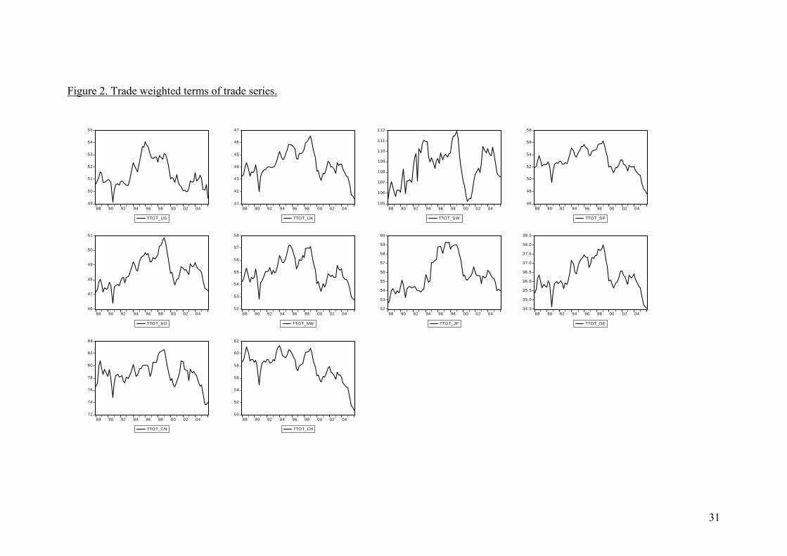
d) Terms of trade differential – This is the log of the terms of trade index of a particular

country expressed as a proportion of the sum of trade weighted terms of trade indices of

the remaining nine countries. Figure 2 in the appendix provides the plots of these series.

e) GDP Per capita differential – This is the log of real GDP per capita of a particular

country expressed as a proportion of the sum of trade-weighted real GDP per capita of

the remaining nine countries. The plots for these series are found in Figure 3 of the

appendix.

In this paper we use two estimators to construct our BEER estimates: the

multivariate cointegration estimator of Johansen (1995) and a Panel DOLS estimator.

12

Since the former estimator is now well know we do not discuss it further here. The latter

estimator, which is perhaps not so well known, has the following form:

1 2 3 4 ,

n

it i t it j i t j itj p

y x xθ θ θ θ ω+

+=−

= + + + Δ +∑ .

Where yit is a scalar, xit is a vector with dimension k, θ1i is an individual fixed effect, θ2t is

a time effect θ3 represents a cointegrating vector, p is the maximum lag length and n is

the maximum lag lead and ω is a Guassian vector error process. The leads and lags of the

first differences are included to orthogonalise the error term.

4. Econometric Results

The single country BEER estimates derived using the multivariate cointegration

methods of Johansen are given in Table 1. The Table should be read in the following

way: Columns 2 to 4 give the coefficient values of the listed variables (with t-ratios in

parenthesis); column 5 indicates if cointegration exists (with the number of cointegrating

vectors in brackets); the final column indicates the coefficient, and associated t-ratio, of

the alpha coefficient on the error correction term in the dynamic exchange rate equation;

the row headings indicate the country in question.

All of the estimates shown in Table 1 indicate the existence of one significant

cointegrating vector for each of the countries and all of the systems produce a negative

loading terms in the exchange rate relationship and all apart from two of these terms are

statistically significant. Apart from the UK, the coefficients on the trade balance term are

statistically negative. We now turn to a more detailed discussion of the results. For

Canada, all of the coefficients are correctly signed and statistically significant. Although

the coefficient on the relative productivity term is wrongly signed in terms of the standard

13

neoclassical (Balassa-Samuelson) framework, it is correctly signed in terms of the more

recent theoretical interpretation of the effects of productivity on the exchange rate (see,

for example, MacDonald and Ricci (2002)). The coefficient on the trade balance suggest

that a one percent reduction in the trade surplus requires a 4.13 appreciation of the log of

the real effective exchange rate. Note that although the mean reversion speed for Canada

is negative, it is also insignificant, a fact that we attribute to the relatively short data span.

With the exception of the interest rate term, all of the coefficients are correctly signed in

the Chinese BEER relationship and the coefficient on the trade balance is very large,

suggesting a very large movement in the real exchange rate is required to adjust the trade

balance. The mean reversion coefficient is significantly negative in the Chinese case.

The results for Germany, reported in Table 1, have the coefficient on the trade

balance term significantly negative, suggesting that a one percent change in the German

trade balance requires a 3 per cent change in the real exchange rate. Other coefficients in

the German equation are insignificant, although the mean reversion coefficient is

statistically significant. The Japanese estimates produce a very large, in absolute terms,

coefficient on the trade balance and a significantly negative mean reversion term. The

results for the Norwegian effective give a significantly negative coefficient on the trade

balance term of –1.53; other coefficients in this relationship are either wrongly signed or

insignificant, although there is clear evidence of significant error correction. The

coefficient on the trade balance for Singapore is in the ball-park of the Canadian and

German estimates being approximately minus 2.5 and statistically significant. Other

coefficients are statistically significant in the Singapore case including the mean

reversion speed.

14

Both Sweden and Switzerland have significantly negative coefficients on their

trade balance terms of –4.52 and -1.85, respectively with other coefficients being

something of a mixed bag; mean reversion speeds are both significant and Switzerland

has the second highest adjustment of any of the countries. The UK results are something

of an outlier in the sense that the coefficient on the trade balance term is positive,

although insignificantly so, and it produces the largest alpha term, in absolute terms, of

any of the countries. The results for the United States indicate a coefficient on the trade

balance of around -1.3, with a t-ratio that is only slightly above one; the coefficients on

the productivity and real interest rate terms are significant although that on the real

interest rate is wrongly signed. The mean reversion speed for the US although correctly

signed is statistically insignificant. We argue that the variance between these results and

those of Clark and MacDonald (1999) can be attributed to the relatively short time series

dimension of the data.

The panel DOLS estimates are presented in Tables 2 through 4. In columns two

and three of Table 2 the results for the full sample of 10 countries, with the full time

sample, are presented, with and without time dummies. In both specifications the

coefficient on the trade balance term enters with the wrong sign and is small in

magnitude, although statistically significant. The coefficients on the relative productivity

and terms of trade variables are correctly signed and significant in both cases. The

coefficient on the real interest rate term is wrongly signed, although insignificant. In

columns 4 and 5 of Table 2 these tests are repeated with the real interest rate term

dropped. The story on the remaining coefficients is essentially unchanged relative to

columns 2 and 3.

15

In Table 3 we present a similar set of panel DOLS estimates for the G3 countries.

Here, strikingly, the coefficient on the trade balance term is significantly negative with a

ball park figure of around 3; that is, a one percentage point improvement in the trade

balance requires a 3 per cent movement in the real exchange rate. Other coefficients

values and their significance are also broadly similar to those reported in Table 2. The

results for the panel of non-G3 countries, reported in Table 4 are in broad conformity

with those reported in Table 2, although the coefficient on the trade balance becomes

statistically insignificant in the specification with time effects.

Our panel DOLS estimates are broadly similar to those reported in Lane and

Milesi-Ferretti (2002) for a panel of 20 countries over the period 1970 to 1998.

Specifically, they find a statistically significant coefficient on the trade balance of around

-6 for the G3, but a statistically insignificant, although negative, coefficient of -0.3 for the

non-G3 (with the full sample being a significant and -0.72).

5. BEER Estimates and Target Current Accounts

The simulation exercises are reported in Table 5 for the scenarios I to III in Williamson

(2006). Scenario I involves the identified surplus countries reducing the size of their

surpluses by 41% of their predicted 2011 values, the US cutting its deficit to 3% of GDP

and other deficit areas staying the same. In Scenario II the surplus countries cut their

surplus to 1.1% of GDP. Scenario III, which takes some account of welfare maximising

objectives, has China and Malaysia moving to a zero current balance. The other surplus

countries, are assumed to have the same current account surplus as in the base case and

the remaining adjustment needed to achieve a similar residual to Scenario I is spread

16

evenly over the other surplus areas, with the two oil exporters expected to adjust by only

one-half as much as the other countries.

Our results are based on the implied trade balance changes necessary to achieve

the above scenarios (in terms of trade balance adjustment, rather than current account

adjustment) using the coefficients on the trade balance reported in Tables 1 and 3. For all,

countries apart from Japan, we use the point estimates from Table 1 and for Japan we use

the point estimate from the panel G3 results (Table 3). For the United States we report

two estimates – one based on the point estimated of -1.3 (Table 1) and the other based on

the G3 estimate of -3.

All of the scenarios show dramatic devaluations for the renminbi, ranging from

27.3 per cent in Scenario I to 46.6 in Scenario III, which requires China to move to a zero

current account position. For the United States, the implied devaluations are between 5

and 11 per cent depending on the point estimates used in the evaluation (see above).

Interestingly, for both the Euro area and the UK effectively no adjustment is required,

suggesting that appropriate adjustment has already taken place for these countries. The

suggested adjustment of the Japanese yen is approximately 6 per cent in each of the

scenarios.

6. Summary and Conclusions

In this paper we have estimated behaviour equilibrium exchange rates for the effective

exchange rates of ten industrialised and emerging market economies that rank within the

top 15 contributory economies to global imbalances. The sample period is 1988, quarter 1

to 2006 quarter 1. The conditioning variables used in the estimation of the BEER are: net

exports as a proportion of GDP, a real interest differential, a terms of trade differential

17

and GDP per capita differential. The ‘foreign’ magnitudes in the differentials were

constructed using the trade weights used to construct the effective exchange rates. Using

both single country and panel econometric methods, plausible BEER estimates were

reported. These estimates were then used to back out the required exchange rate

adjustments necessary to fulfil the three scenarios of Williamson (2006). The ball park

currency adjustment required are in the range of 27.3 to 46.6 per cent for the Chinese

renminbi, 5 to 11 per cent for the US dollar, approximately 6 per cent for he Japanese yen

and no adjustment for the euro or Sterling.

18

References

Clark, P.B. and R. MacDonald, (1999), “Exchange Rates and Economic Fundamentals: A Methodological Comparison of BEERs and FEERs” in R. MacDonald and J Stein (eds) Equilibrium Exchange Rates, Kluwer: Amsterdam. And IMF Working Paper 98/67 (Washington: International Monetary Fund, March 1998)

Clark, P.B. and R. MacDonald, (2000), “Filtering the BEER a permanent and transitory

decomposition’, IMF Working Paper 00/144 (Washington: International Monetary Fund) and Global Finance Journal

Égert, B. and L. Halpern and R. MacDonald (2006), ‘Equilibrium Exchange Rates in

Transition Economies: Taking Stock of the Issues’, Journal of Economic Surveys.

Faruqee, H., “Long-Run Determinants of the Real Exchange Rate: A Stock-Flow

Perspective”, Staff Papers, International Monetary Fund, Vol. 42 (March 1995), pp. 80-107.

Faruqee, H., P. Isard, and P.R. Masson (1998), A Macroeconomic Balance Framework

for Estimating Equilibrium Exchange Rates, R MacDonald and J Stein, (eds) Equilibrium Exchange Rates, chapter 4. Boston: Kluwer.

Johansen, S. (1995), Likelihood-based Inference in Cointegrated Vector Autoregressive

Models, Oxford: Oxford University Press. Lane, Philip R., and Gian Maria Milesi-Ferretti, (2001), “The External Wealth of

Nations: Measures of Foreign Assets and Liabilities for Industrial and Developing Countries,” Journal of International Economics, Vol. 55, pp. 263–94.

MacDonald, R. (1998), "What Determines Real Exchange Rates? The Long and the Short

of It", Journal of International Financial Markets, Institutions and Money, 8, 117-153. [reprinted in R. MacDonald and J Stein (eds) Equilibrium Exchange Rates, Kluwer: Amsterdam.]

MacDonald, R. (1999), “Asset Market and Balance of Payments Characteristics: An

Eclectic Exchange Rate Model for the Dollar, Mark, and Yen”, Open Economies Review 10, 1, 5-30.

MacDonald, R. (2007), Exchange Rate Economics: Theories and Evidence (Second

Edition of Floating Exchange Rates: Theories and Evidence), Routledge, 2007.

19

MacDonald, R. and L. Ricci (2002), "Real Exchange Rates, Imperfect Substitutability, and Imperfect Competition", IMF working paper and Journal of Macroeconomics, forthcoming.

Stein, J. (1999), “The Evolution of the Real Value of the US Dollar Relative to the G7

Currencies”, Chapter 3, Equilibirum Exchange Rates, (eds) R. MacDonald and J. Stein. Amsterdam: Kluwer Press.

Williamson, J. (1983), Estimating Equilibrium Exchange Rates, Washington, DC:

Institute for International Economics. Williamson, J. (2006), The target current account outcomes, mimeo, Peterson Institute for

International Economics Wren-Lewis, S. (1992), “On the Analytical Foundations of the Fundamental Equilibrium

Exchange Rate”, in Macroeconomic Modelling of the Long Run (ed.) Colin P. Hargreaves, Edward Elgar.

20

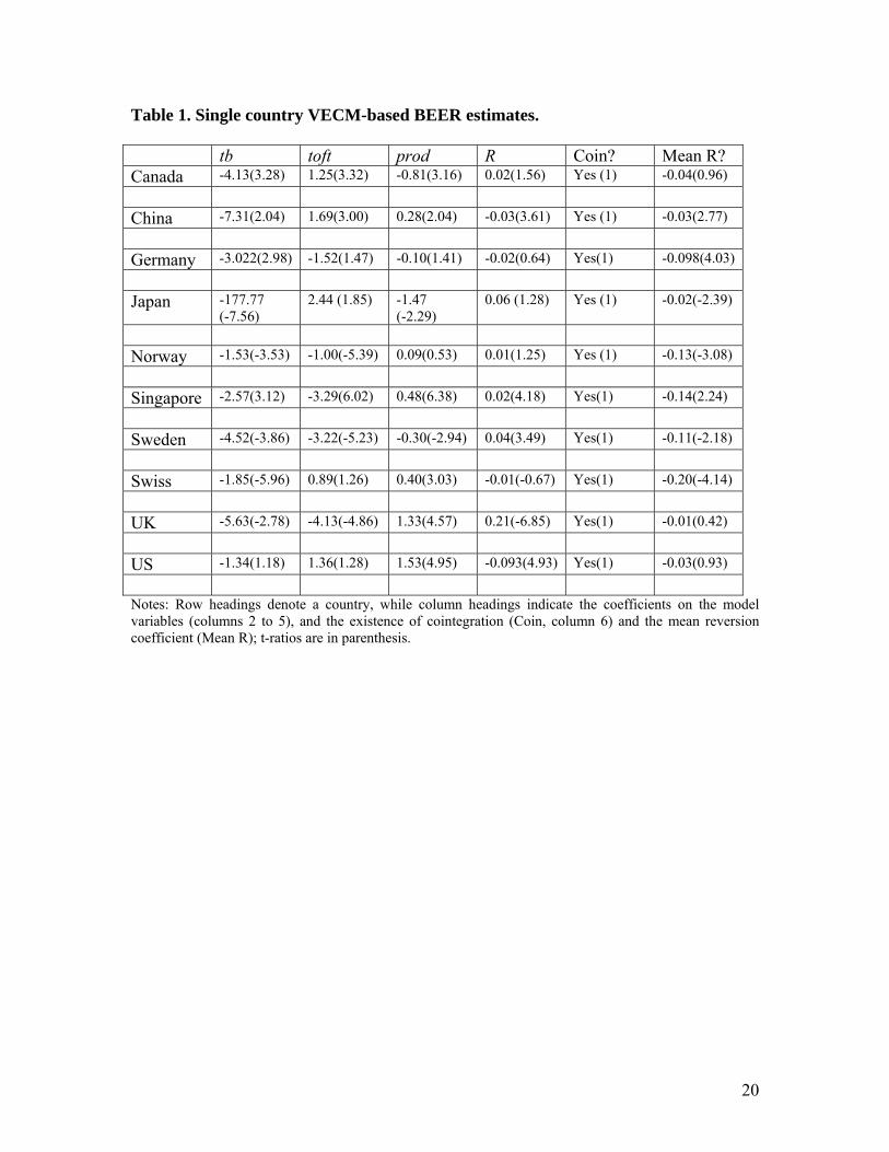
Table 1. Single country VECM-based BEER estimates.

tb toft prod R Coin? Mean R? Canada -4.13(3.28) 1.25(3.32) -0.81(3.16) 0.02(1.56) Yes (1) -0.04(0.96) China -7.31(2.04) 1.69(3.00) 0.28(2.04) -0.03(3.61) Yes (1) -0.03(2.77) Germany -3.022(2.98) -1.52(1.47) -0.10(1.41) -0.02(0.64) Yes(1) -0.098(4.03) Japan -177.77

(-7.56) 2.44 (1.85) -1.47

(-2.29) 0.06 (1.28) Yes (1) -0.02(-2.39)

Norway -1.53(-3.53) -1.00(-5.39) 0.09(0.53) 0.01(1.25) Yes (1) -0.13(-3.08) Singapore -2.57(3.12) -3.29(6.02) 0.48(6.38) 0.02(4.18) Yes(1) -0.14(2.24) Sweden -4.52(-3.86) -3.22(-5.23) -0.30(-2.94) 0.04(3.49) Yes(1) -0.11(-2.18) Swiss -1.85(-5.96) 0.89(1.26) 0.40(3.03) -0.01(-0.67) Yes(1) -0.20(-4.14) UK -5.63(-2.78) -4.13(-4.86) 1.33(4.57) 0.21(-6.85) Yes(1) -0.01(0.42) US -1.34(1.18) 1.36(1.28) 1.53(4.95) -0.093(4.93) Yes(1) -0.03(0.93) Notes: Row headings denote a country, while column headings indicate the coefficients on the model variables (columns 2 to 5), and the existence of cointegration (Coin, column 6) and the mean reversion coefficient (Mean R); t-ratios are in parenthesis.

21

Table 2. Panel Estimates of the BEER model – Full Sample. Full Full Full Full Tb 0.353 (4.41) 0.228 (2.33) 0.363 (4.54) 0.221 (2.30) Prod 0.110 (5.22) 0.104 (4.54) 0.096 (4.75) 0.092 (4.33) Toft 0.511 (9.02) 0.484 (8.09) 0.512 (9.23) 0.489 (8.44) R -0.003 (1.68) -0.002 (0.93) - - Adjusted R2 0.42 0.38 0.42 0.40 Nobs 730 730 730 730 N Countries 10 10 10 10 Time Effects? No Yes No Yes Notes: Equations estimated with a Panel DOLS (1,1) estimator; t-ratios in brackets.

22

Table 3. Panel Estimates of the BEER model – G3 Sample. G3 G3 G3 G3 Tb -2.924 (6.97) -2.916 (4.71) -2.976 (7.04) -2.332 (4.15) Prod 0.122 (3.45) 0.136 (2.29) 0.154 (4.52) 0.092 (1.69) Toft 0.902 (7.35) 0.775 (4.18) 0.756 (6.86) 0.843 (4.53) R -0.012 (2.54) -0.018 (2.09) - - Adjusted R2 0.60 0.57 0.59 0.55 Nobs 210 210 210 210 N Countries 3 3 3 3 Time Effects? No Yes No Yes Notes: Equations estimated with a Panel DOLS (1,1) estimator; t-ratios in brackets.

23

Table 4. Panel Estimates of the BEER model – Non G3 Sample. Non-G3 Non-G3 Non-G3 Non-G3 Tb 0.414 (4.93) 0.179 (1.44) 0.431 (5.12) 0.191 (1.57) Prod 0.109 (4.11) 0.103 (3.58) 0.088 (3.64) 0.083 (3.26) Toft 0.454 (7.11) 0.349 (4.61) 0.467 (7.42) 0.363 (4.97) R -0.002 (1.38) -0.002 (0.96) - - Adjusted R2 0.40 0.37 0.39 0.37 Nobs 511 511 511 210 N Countries 7 7 7 3 Time Effects? No Yes No Yes Notes: Equations estimated with a Panel DOLS (1,1) estimator; t-ratios in brackets.

24

Table 5. Simulations Baseline Country $b %GDP Coefficient of

TB Canada 24 1.8 -4.13 China 224 6.3 -7.4 Germany -23 -0.2 -3.022 Japan 131 3.2 -3 Norway 59 19.4 -1.53 Singapore 39 25.6 -2.57 Sweden 27 7.1 -4.52 Switzerland 44 13.3 -1.85 U.K -67 -2.6 -5.63 U.S -946 -6.8 -1.34/-3 Scenario I Country $b % of GDP Change in the

exchange rate implied by the TB

Canada 10 .75 4.33 China 93 2.61 27.3 Germany/Euro proxy -23 -0.2 - Japan 54 1.31 5.67 Norway 24 7.89 17.6 Singapore 16 10.50 38.8 Sweden 11 2.89 19.02 Switzerland 18 5.44 14.54 U.K -67 -2.6 - U.S -417 -3 5.1/11.4 Scenario II Country $b % of GDP Change in the

exchange rate implied by the TB

Canada 15 1.12 2.9 China 39 1.09 38.5 Germany/Euro proxy -23 -0.2 - Japan 45 1.10 6.3 Norway 3 0.98 28.18 Singapore 2 1.31 22.23 Sweden 4 1.05 27.34 Switzerland 4 1.20 11.00 U.K -67 -2.6 - U.S -417 -3 5.1/11.4

25

Scenario III Country $b % of GDP Change in the

exchange rate implied by the TB

Canada 7 0.52 5.28 China 0 0 46.62 Germany/Euro proxy -23 -0.2 - Japan 36 0.88 6.96 Norway 30 9.86 14.59 Singapore 10 6.56 48.93 Sweden 7 1.84 23.77 Switzerland 13 3.92 17.35 U.K -67 -2.6 - U.S -417 -3 5.09/11.4 Notes: See section 5 for an explanation of scenarios.

26

27

Data Appendix. A. Data Sources

Country Frequency Data Field Data Source U.S Quarterly REER IFS Statistics November 2006 Do CPI Do Do C/A Do Do Bond Yield Do Do GDP Do Do Trade Balance Do Annual GDP Per capita Data Stream – Economic Intelligence Unit Monthly Terms of Trade Data Stream Latest Update* Trade Weights IMF China Quarterly REER IFS Statistics November 2006 Do CPI Do Annual C/A Data Stream – State Administration of foreign exchange. BOP C/A goods & services Quarterly Bond Yield IFS Statistics November 2006 Annual GDP Data Stream – OECD Main economic indicators Quarterly Trade Balance Data Stream – OECD Main economic indicators Do Foreign exchange rate IFS Statistics November 2006 Annual GDP Per capita Data Stream – Economic Intelligence Unit Annual Terms of Trade Data Stream Latest Update* Trade Weights IMF Japan Quarterly REER IFS Statistics November 2006 Do CPI Do Do C/A Do Do Bond Yield Do Do GDP Do Do Trade Balance Do Do Foreign exchange rate Do Annual GDP Per capita Data Stream – Economic Intelligence Unit Monthly Terms of Trade Data Stream Latest Update* Trade Weights IMF U.K Quarterly REER IFS Statistics November 2006 Do CPI Do Do C/A Do Do Bond Yield Do Do GDP Do Do Trade Balance Do Do Foreign exchange rate Do Annual GDP Per capita Data Stream – Economic Intelligence Unit Monthly Terms of Trade Data Stream Latest Update* Trade Weights IMF Norway Quarterly REER IFS Statistics November 2006 Do CPI Do Annual C/A Data Stream - IFS Quarterly Bond Yield IFS Statistics November 2006 Do GDP Do Do Trade Balance Data Stream – Statistics Norway - BOP external trade balance Do Foreign exchange rate IFS Statistics November 2006 Annual GDP Per capita Data Stream – Economic Intelligence Unit Quarterly Terms of Trade Data Stream Latest Update* Trade Weights IMF Switzerland Quarterly REER IFS Statistics November 2006 Do CPI Do Do C/A Data Stream – OECD Main Economic Indicators Do Bond Yield IFS Statistics November 2006 Do GDP Do Monthly Trade Balance Data Stream – OECD Main Economic Indicators Quarterly Foreign exchange rate IFS Statistics November 2006 Annual GDP Per capita Data Stream – Economic Intelligence Unit Monthly Terms of Trade Data Stream Latest Update* Trade Weights IMF Singapore Quarterly REER IFS Statistics November 2006 Do CPI Do Do C/A Data Stream – Department of Statistics, Singapore Do Bond Yield IFS Statistics November 2006 Annual GDP Data Stream - IFS

28

Quarterly Trade Balance Data Stream – Department of Statistics, Singapore Do Foreign exchange rate IFS Statistics November 2006 Annual GDP Per capita Data Stream – Economic Intelligence Unit Quarterly Terms of Trade Data Stream Latest Update* Trade Weights IMF Sweden Quarterly REER IFS Statistics November 2006 Do CPI Do Do C/A Do Do Bond Yield Do Do GDP Do Do Trade Balance Do Do Foreign exchange rate Do Annual GDP Per capita Data Stream – Economic Intelligence Unit Quarterly Terms of Trade Data Stream Latest Update* Trade Weights IMF Canada Quarterly REER IFS Statistics November 2006 Do CPI Do Do C/A Do Do Bond Yield Do Do GDP Do Do Trade Balance Do Do Foreign exchange rate Do Annual GDP Per capita Data Stream – Economic Intelligence Unit Quarterly Terms of Trade Data Stream Latest Update* Trade Weights IMF Germany Quarterly REER IFS Statistics November 2006 Do CPI Do Do C/A Do Do Bond Yield Do Do GDP Do Do Trade Balance Do Do Foreign exchange rate Do Annual GDP Per capita Data Stream – Economic Intelligence Unit Monthly Terms of Trade Data Stream Latest Update* Trade Weights IMF * Data pertains to the following IMF working paper: New Rates from New Weights (2005) Tamim Bayoumi, Jaewoo Lee and Sarma Jayanthi

29

B. Trade Weights Canada China Germany Japan Norway Singapore Sweden Switzerland U.K U.S Canada 0 0.028256 0.029067 0.045311 0.002132 0.004731 0.004787 0.004741 0.023324 0.654722 China 0.023439 0 0.064829 0.191924 0.003089 0.01916 0.009052 0.0077 0.027591 0.233493 Germany 0.012103 0.032693 0 0.05134 0.006109 0.008546 0.019885 0.039132 0.074472 0.121463 Japan 0.022825 0.117231 0.062016 0 0.003599 0.028099 0.008381 0.010527 0.034091 0.272602 Norway 0.014614 0.02783 0.124426 0.05322 0 0.006205 0.0128821 0.012491 0.087081 0.095347 Singapore 0.011199 0.060029 0.051286 0.144582 0.001822 0 0.005185 0.009106 0.036802 0.206135 Sweden 0.013471 0.031743 0.139101 0.048068 0.042452 0.006024 0 0.016651 0.081927 0.0108335Switzerland 0.011188 0.022231 0.227298 0.05038 0.003706 0.008788 0.013824 0 0.64554 0.111696 U.K 0.016987 0.025143 0.137264 0.051269 0.007735 0.011185 0.021659 0.020508 0 0.150011 U.S 0.1482 0.066396 0.067989 0.12765 0.00282 0.018787 0.008722 0.010819 0.04583 0 * Data pertains to the following IMF working paper: New Rates from New Weights (2005) Tamim Bayoumi, Jaewoo Lee and Sarma Jayanthi

30

Figure 1. Trade weighted real interest rate series.

1.0

1.5

2.0

2.5

3.0

3.5

4.0

4.5

88 90 92 94 96 98 00 02 04

TRINT_CH

1

2

3

4

5

6

7

88 90 92 94 96 98 00 02 04

TRINT_CN

0.4

0.8

1.2

1.6

2.0

2.4

2.8

3.2

88 90 92 94 96 98 00 02 04

TRINT_DE

0

1

2

3

4

5

88 90 92 94 96 98 00 02 04

TRINT_JP

1.2

1.6

2.0

2.4

2.8

3.2

3.6

4.0

4.4

4.8

88 90 92 94 96 98 00 02 04

TRINT_NW

1.0

1.5

2.0

2.5

3.0

3.5

4.0

88 90 92 94 96 98 00 02 04

TRINT_SD

0.8

1.2

1.6

2.0

2.4

2.8

3.2

3.6

4.0

88 90 92 94 96 98 00 02 04

TRINT_SP

3

4

5

6

7

8

9

10

11

88 90 92 94 96 98 00 02 04

TRINT_SW

0.5

1.0

1.5

2.0

2.5

3.0

3.5

88 90 92 94 96 98 00 02 04

TRINT_UK

0.8

1.2

1.6

2.0

2.4

2.8

3.2

3.6

4.0

88 90 92 94 96 98 00 02 04

TRINT_US

31

Figure 2. Trade weighted terms of trade series.

49

50

51

52

53

54

55

88 90 92 94 96 98 00 02 04

TTOT_US

41

42

43

44

45

46

47

88 90 92 94 96 98 00 02 04

TTOT_UK

105

106

107

108

109

110

111

112

88 90 92 94 96 98 00 02 04

TTOT_SW

46

48

50

52

54

56

58

88 90 92 94 96 98 00 02 04

TTOT_SP

46

47

48

49

50

51

88 90 92 94 96 98 00 02 04

TTOT_SD

52

53

54

55

56

57

58

88 90 92 94 96 98 00 02 04

TTOT_NW

52

53

54

55

56

57

58

59

60

88 90 92 94 96 98 00 02 04

TTOT_JP

34.5

35.0

35.5

36.0

36.5

37.0

37.5

38.0

38.5

88 90 92 94 96 98 00 02 04

TTOT_DE

72

74

76

78

80

82

84

88 90 92 94 96 98 00 02 04

TTOT_CN

50

52

54

56

58

60

62

88 90 92 94 96 98 00 02 04

TTOT_CH

32

Figure 3. Trade weighted real GDP percapita series.

14000

15000

16000

17000

18000

19000

20000

21000

88 90 92 94 96 98 00 02 04

TCAP3_CH

22000

23000

24000

25000

26000

27000

28000

29000

30000

31000

88 90 92 94 96 98 00 02 04

TCAP3_CN

9000

9500

10000

10500

11000

11500

12000

12500

13000

88 90 92 94 96 98 00 02 04

TCAP3_DE

11000

12000

13000

14000

15000

16000

17000

88 90 92 94 96 98 00 02 04

TCAP3_JP

12000

13000

14000

15000

16000

17000

18000

19000

88 90 92 94 96 98 00 02 04

TCAP3_NW

9000

10000

11000

12000

13000

14000

15000

16000

17000

88 90 92 94 96 98 00 02 04

TCAP3_SD

11000

12000

13000

14000

15000

16000

17000

88 90 92 94 96 98 00 02 04

TCAP3_SP

20000

24000

28000

32000

36000

40000

88 90 92 94 96 98 00 02 04

TCAP3_SW

9000

10000

11000

12000

13000

14000

15000

16000

88 90 92 94 96 98 00 02 04

TCAP3_UK

9000

10000

11000

12000

13000

14000

15000

88 90 92 94 96 98 00 02 04

TCAP3_US

33

Figure 4. Log of REERs.

4.2

4.3

4.4

4.5

4.6

4.7

4.8

88 90 92 94 96 98 00 02 04

LREER_CH

4.50

4.55

4.60

4.65

4.70

4.75

4.80

88 90 92 94 96 98 00 02 04

LREER_CN

4.45

4.50

4.55

4.60

4.65

4.70

4.75

4.80

4.85

88 90 92 94 96 98 00 02 04

LREER_DE

4.2

4.3

4.4

4.5

4.6

4.7

4.8

4.9

88 90 92 94 96 98 00 02 04

LREER_JP

4.3

4.4

4.5

4.6

4.7

4.8

4.9

88 90 92 94 96 98 00 02 04

LREER_NW

4.48

4.52

4.56

4.60

4.64

4.68

4.72

4.76

4.80

4.84

88 90 92 94 96 98 00 02 04

LREER_SD

4.40

4.45

4.50

4.55

4.60

4.65

4.70

4.75

88 90 92 94 96 98 00 02 04

LREER_SP

4.4

4.5

4.6

4.7

4.8

88 90 92 94 96 98 00 02 04

LREER_SW

4.2

4.3

4.4

4.5

4.6

4.7

88 90 92 94 96 98 00 02 04

LREER_UK

4.35

4.40

4.45

4.50

4.55

4.60

4.65

4.70

4.75

88 90 92 94 96 98 00 02 04

LREER_US