Belief Dispersion in the Stock Market∗

Adem Atmaz

Krannert School of Management

Purdue University

Suleyman Basak

London Business School

and CEPR

This Version: September 2015

Abstract

We develop a dynamic model of belief dispersion which simultaneously explains the empiricalregularities in a stock price, its mean return, volatility, and trading volume. Our model with acontinuum of (possibly Bayesian) investors differing in beliefs is tractable and delivers exact closed-form solutions. Our model has the following implications. We find that the stock price is convexin cash-flow news, and it increases in belief dispersion while its mean return decreases when theview on the stock is optimistic, and vice versa when pessimistic. We also show that the presenceof belief dispersion generates excess stock volatility, non-trivial trading volume, and a positiverelation between these two quantities. Moreover, we find that the investors’ Bayesian learninginduces less excess volatility when belief dispersion is higher. Furthermore, we demonstrate thatthe more familiar, otherwise identical, finitely-many-investor models of heterogeneous beliefs donot necessarily generate our main results.

JEL Classifications: D53, G12.Keywords: Asset pricing, belief dispersion, stock price, mean return, volatility, trading volume,Bayesian learning.

∗Email addresses: aatmaz@purdue.edu and sbasak@london.edu. We thank Andrea Buffa, GeorgyChabakauri, Francisco Gomes, Christian Heyerdahl-Larsen, Ralph Koijen, Hongjun Yan and our discussantsMina Lee, Daniel Andrei, Philipp Illeditsch and Tim Johnson as well as the seminar participants at the 2015SFS Finance Cavalcade, 2015 WFA meetings, 2015 EFA meetings, 2015 Wabash River Finance Conference andLondon Business School for helpful comments. All errors are our responsibility.

1 Introduction

The empirical evidence on the effects of investors’ dispersion of beliefs on asset prices and their

dynamics is vast and mixed. For example, several works find a negative relation between belief

dispersion and a stock mean return (Diether, Malloy, and Scherbina (2002), Chen, Hong, and

Stein (2002), Goetzmann and Massa (2005), Park (2005), Berkman, Dimitrov, Jain, Koch, and

Tice (2009), Yu (2011)). Others argue that the negative relation is only valid for stocks with

certain characteristics (e.g., small, illiquid, worst-rated or short sale constrained) and in fact,

find either a positive or no significant relation (Qu, Starks, and Yan (2003), Doukas, Kim, and

Pantzalis (2006), Avramov, Chordia, Jostova, and Philipov (2009)). Existing theoretical works,

on the other hand, do not provide satisfactory answers for these mixed results. In fact, most

studies find belief dispersion to be an extra risk factor for investors, and therefore generate only

a positive dispersion-mean return relation.1

In this paper, we develop a tractable model of belief dispersion which is able to simultane-

ously support the empirical regularities in a stock price, its mean return, volatility, and trading

volume. To our knowledge this is the first paper accomplishing this. Towards that, we develop a

dynamic general equilibrium model populated by a continuum of constant relative risk aversion

(CRRA) investors who differ in their (dogmatic or Bayesian) beliefs. Our model delivers fully

closed-form expressions for all quantities of interest.

In our analysis, we summarize the wide range of investors’ beliefs by two sufficient measures,

the average bias and dispersion in beliefs, and demonstrate that equilibrium quantities are

driven by these two key endogenous variables. We take the average bias to be the bias of

the representative investor whereby how much an investor’s belief contributes to the average

bias depends on her wealth and risk attitude. Investors whose beliefs get supported by actual

cash-flow news become relatively wealthier through their investment in the stock, and therefore

contribute more to the average bias. This leads to fluctuations in the average bias so that

following good (bad) cash-flow news, the view on the stock becomes relatively more optimistic

(pessimistic). On the other hand, consistently with empirical studies, we construct our belief

dispersion measure as the cross-sectional standard deviation of investors’ disagreement which

also enables us to uncover its dual role. First, we show that belief dispersion amplifies the

current average bias so that the same good (bad) news leads to more optimism (pessimism)

when dispersion is higher. Second, we show that belief dispersion indicates how much the

average bias fluctuates, and therefore measures the extra uncertainty investors face.

1We discuss the theoretical literature in detail in Section 1.1.

1

Turning to stock market implications, we first find that in the presence of belief dispersion

the stock price is convex in cash-flow news, indicating that the stock price is more sensitive to

news in relatively good states. It also implies that the increase in the stock price following good

news is more than the decrease following bad news, as supported by empirical evidence (Basu

(1997), Xu (2007)). Convexity arises because, the better the cash-flow news, the higher the

extra boost for the stock price coming from elevated optimism. Consequently, the stock price

increases with belief dispersion when the view on the stock is relatively optimistic, and decreases

otherwise, also consistent with empirical evidence (Yu (2011)). Our model also generates a novel

implication that the stock price may increase and its mean return may decrease in investors’

risk aversion in relatively bad states. This is because bad news leads to less pessimism in a

more risk averse economy. More risk averse investors have less exposure to the stock which

reduces the wealth transfers to pessimistic investors in bad times.

We next examine the widely-studied relation between belief dispersion and a stock mean

return. Since dispersion represents additional risk for investors, risk averse investors demand a

higher return to hold the stock when dispersion is higher. However, dispersion also amplifies

optimism and pushes up the stock price following good news leading to a lower mean return

in those states. When the view on the stock is relatively optimistic, the second effect domi-

nates and we find a negative dispersion-mean return relation. As discussed earlier, empirical

evidence on this relation is mixed, with some studies finding a negative while others finding

a positive or no significant relation. Our model generates both possibilities and demonstrates

that this relation is negative when the view on the stock is relatively optimistic, and positive

otherwise. Diether, Malloy, and Scherbina (2002) provide supporting evidence to our finding

by documenting an optimistic bias in their study overall, and by also showing that the negative

effect of dispersion becomes stronger for more optimistic stocks.

We further find that the presence of belief dispersion generates excess volatility by increas-

ing the stock volatility beyond its fundamental uncertainty. This is because investors face

the additional risk of stochastic average bias in beliefs, which then amplifies the stock price

fluctuations, inducing excess volatility. Obviously, the higher the belief dispersion, the higher

the excess stock volatility, which is also consistent with empirical evidence (Ajinkya and Gift

(1985), Anderson, Ghysels, and Juergens (2005), Banerjee (2011)). In addition to belief dis-

persion, the investors’ Bayesian learning process also increases the fluctuations of the average

bias in beliefs. This occurs because all investors become relatively more optimistic (pessimistic)

following good (bad) news due to belief updating. In the literature, both the belief dispersion

and learning channels are proposed as explanations for the excess stock volatility, among oth-

2

ers. Our closed-form stock volatility expression allows us to disentangle their respective effects,

and yields a novel testable implication that the investors’ Bayesian learning induces less excess

volatility when belief dispersion is higher.

We also examine the effects of belief dispersion on the stock trading volume and find that the

trading volume is increasing in dispersion, consistently with empirical evidence (Ajinkya, Atiase,

and Gift (1991), Bessembinder, Chan, and Seguin (1996), Goetzmann and Massa (2005)). This

finding is intuitive since when dispersion is higher, investors with relatively different beliefs,

who also have relatively higher trading demands, are more dominant. We also find a positive

relation between the stock volatility and trading volume due to the positive effect of dispersion

on both quantities, which is also supported empirically (Gallant, Rossi, and Tauchen (1992)).

Finally, we demonstrate that most of our results above do not necessarily obtain in the

more familiar, otherwise identical, finitely-many agent economies with heterogeneous beliefs.

In particular, we show that in these economies, the stock price may no longer be convex in cash-

flow news across all states of the world, and a higher belief dispersion has ambiguous effects on

the stock volatility and trading volume, in contrast to our model implications. This happens

because in these economies, unlike in our model, belief heterogeneity effectively vanishes in

relatively extreme states, which forces these models to be dominated by a particular type of

agent and to have implications similar to those in a homogeneous agent economy in those states,

yielding irregular behavior for economic quantities.

1.1 Related Theoretical Literature

In this paper, we solve a dynamic heterogeneous beliefs model with a continuum of, possibly

Bayesian, investors having general CRRA preferences, and obtain fully closed-form solutions for

all quantities of interest. Generally, these models are hard to solve for long-lived assets beyond

logarithmic preferences (e.g., Detemple and Murthy (1994), Zapatero (1998), Basak (2005)).

Our methodological contribution and the tractability of our model is in large part due to the

investor types having a Gaussian distribution. This assumption follows from the recent works

by Cvitanic and Malamud (2011) and Atmaz (2014). Cvitanic and Malamud does not consider

the average bias and dispersion in beliefs and focuses on the survival and portfolio impact

of irrational investors, while Atmaz does, but employs logarithmic preferences and focuses on

short interest.

The literature on heterogeneous beliefs in financial markets is vast. There are two key differ-

ences between our model and earlier works which enable our model to simultaneously support

3

the empirical regularities. First, most of the earlier works are set in a two-agent framework, and

usually consider the overall effects of belief heterogeneity rather than decomposing its effects

due to average bias and dispersion in beliefs, as we do. This is notable because it enables us

to isolate the effects of dispersion from the effects of other moments and conduct comparative

statics analysis with respect to belief dispersion only, resulting in sharp results.2 Second and

more importantly, as discussed above, in our model no investor dominates the economy in rel-

atively extreme states, which otherwise may lead to irregular behavior for economic quantities

as we demonstrate in Sections 4.3 and 5.3.

One strand of the extensive heterogeneous beliefs literature examines the relation between

belief dispersion and stock mean return. As discussed earlier, most studies find this relation to

be positive (e.g., Abel (1989), Anderson, Ghysels, and Juergens (2005), David (2008), Banerjee

and Kremer (2010)). On the other hand, Chen, Hong, and Stein (2002) and Johnson (2004)

establish a negative relation by imposing short selling constraints for certain type of investors

and considering levered firms, respectively. Buraschi, Trojani, and Vedolin (2013) develop a

credit risk model and show that an increasing heterogeneity of beliefs has a negative (positive)

effect on the mean return for firms with low (high) leverage. However, this result does not hold

for unlevered firms. Differently from these works, we show that the dispersion-mean return

relation is negative when the view on the stock is relatively optimistic and positive otherwise.

Another strand in the heterogeneous beliefs literature examines the impact of belief disper-

sion on stock volatility and typically finds a positive effect (e.g., Scheinkman and Xiong (2003),

Buraschi and Jiltsov (2006), Li (2007), David (2008), Dumas, Kurshev, and Uppal (2009),

Banerjee and Kremer (2010), Andrei, Carlin, and Hasler (2015)). Yet another strand in this

literature employs belief dispersion models to explain empirical regularities in trading volume.

Early works include Harris and Raviv (1993) and Kandel and Pearson (1995). This strand also

includes the works which find a positive relation between belief dispersion and trading volume,

as in our work (e.g., Varian (1989), Shalen (1993), Cao and Ou-Yang (2008), Banerjee and Kre-

mer (2010)). Even though our paper differs from each one of these papers in several aspects,

one common difference is that none of the above papers generate the stock price convexity as

in our model.3

2Moreover, in models with two agents, belief heterogeneity is typically defined as the difference in beliefs ofthese agents which cannot readily be extended to an economy with many agents. By taking belief dispersionto be the cross-sectional standard deviation of investors’ disagreement, our measure can be employed for anarbitrary investor population, but also captures the heterogeneity in beliefs when specialized to a two-agenteconomy (due to the monotonicity between differences in beliefs and the standard deviation of disagreement).

3Other works studying the effects of heterogeneous beliefs in financial markets include Basak (2000), Kogan,Ross, Wang, and Westerfield (2006), Jouini and Napp (2007), Gallmeyer and Hollifield (2008), Yan (2008),Xiong and Yan (2010), Bhamra and Uppal (2014), Chabakauri (2015). We note that as in most of above works,

4

Finally, this paper is also related to the literature on parameter uncertainty and Bayesian

learning. In this literature, Veronesi (1999) and Lewellen and Shanken (2002) show that learn-

ing leads to stock price overreaction, time-varying expected returns and excess volatility. In

particular, Veronesi shows that the stock price overreaction leads to a convex stock price.4

Timmermann (1993, 1996), Barsky and De Long (1993), Brennan and Xia (2001), Pastor

and Veronesi (2003) show that learning generates excess volatility and predictability for stock

returns. However, differently from our work, all these works employ homogeneous investors

setups, and therefore are not suitable for studying the effects of belief dispersion.

The remainder of the paper is organized as follows. Section 2 presents the simpler dogmatic

beliefs version of our model which also serves to demonstrate that our results are not driven

by Bayesian learning. Section 3 analyzes the average bias and dispersion in beliefs. Section 4

presents our results for the stock price and its mean return, while Section 5 those for the stock

volatility and trading volume. Section 6 presents our general model with Bayesian learning

and shows that all our results remain valid in this more complex economy. Section 7 concludes

the paper. Appendix A contains the proofs of the dogmatic beliefs model and introduces the

finitely-many-investor version of our model. Internet Appendix B contains the proofs of our

general model with Bayesian learning.

2 Economy with Dispersion in Beliefs

We consider a simple and tractable pure-exchange security market economy with a finite horizon

evolving in continuous time. The economy is assumed to be large as it is populated by a

continuum of investors with heterogeneous beliefs and standard CRRA preferences. In the

general specification of our model, investors optimally learn over time in a Bayesian fashion.

However, to highlight that our results are not driven by parameter uncertainty and learning,

we first consider the economy when all investors have dogmatic beliefs. The richer case when

investors update their beliefs over time is relegated to Section 6. We show that all our results

hold in this more complex economy.

our investors have symmetric information and their disagreement is due to their different priors, unlike in otherworks where investors’ disagreement is due to their asymmetric information (e.g., Grossman and Stiglitz (1980),Biais, Bossaerts, and Spatt (2010)).

4In Veronesi (1999) the stock price convexity arises due to parameter uncertainty and the learning process,whereas in our model the convexity follows from the stochastic average bias in beliefs, which is due to theendogenous wealth transfers among heterogeneous investors and obtains even when there is no parameter un-certainty and learning. In more recent work, Xu (2007) develops a model in which the stock price is a convexfunction of the public signal. However, in his model no-short-sales constraints are needed to obtain this resultand he does not investigate the stock mean return and volatility as we do.

5

2.1 Securities Market

There is a single source of risk in the economy which is represented by a Brownian motion ω

defined on the true probability measure P. Available for trading are two securities, a risky stock

and a riskless bond. The stock price S is posited to have dynamics

dSt = St [µStdt+ σStdωt] , (1)

where the stock mean return µS and volatility σS are to be endogenously determined in equi-

librium. The stock market is in positive net supply of one unit and is a claim to the payoff DT ,

paid at some horizon T , and so ST = DT . This payoff DT is the horizon value of the cash-flow

news process Dt with dynamics

dDt = Dt [µdt+ σdωt] , (2)

where D0 = 1, and µ and σ are constant, and represent the true mean growth rate of the

expected payoff and the uncertainty about the payoff, respectively. The bond is in zero net

supply and pays a riskless interest rate r, which is set to 0 without loss of generality.5

2.2 Investors’ Beliefs

There is a continuum of investors who commonly observe the same cash-flow news process D

(2), but have different beliefs about its dynamics. The investors are indexed by their type θ,

where a θ-type investor agrees with others on the stock payoff uncertainty σ but believes that

the mean growth rate of the expected payoff is µ+ θ instead of µ. This allows us to interpret a

θ-type investor as an investor with a bias of θ in her beliefs. Consequently, a positive (negative)

bias for an investor implies that she is relatively optimistic (pessimistic) compared to an investor

with true beliefs. Under the θ-type investor’s beliefs, the cash-flow news process has dynamics

dDt = Dt [(µ+ θ) dt+ σdωt (θ)] ,

where ω (θ) is her perceived Brownian motion with respect to her own probability measure Pθ,

and is given by ωt (θ) = ωt − θt/σ. Similarly, the risky stock price dynamics as perceived by

the θ-type investor follows

dSt = St [µSt (θ) dt+ σStdωt (θ)] , (3)

5Since investors have preferences only over horizon wealth, the interest rate can be taken exogenously. Ournormalization of zero interest rate is for expositional simplicity and it is commonly employed in models with nointermediate consumption, see, for example, Pastor and Veronesi (2012) for a recent reference.

6

which together with the dynamics (1) yields the following consistency relation between the

perceived and true stock mean returns for the θ-type investor

µSt (θ) = µSt + σStθ

σ. (4)

The investor type space is denoted by Θ and it is taken to be the whole real line R to

incorporate all possible beliefs including the extreme ones and to avoid having arbitrary bounds

for investor biases. We assume a Gaussian distribution with mean m and standard deviation

v for the relative frequency of investors over the type space Θ. This assumption ensures that

the investor population has a finite (unit) measure and admits much tractability, and can be

justified on the grounds of the typical investor distribution observed in well-known surveys.6

We further assume that all investors are initially endowed with an equal fraction of stock shares.

Since a group of investors with the same beliefs and endowments are identical in every aspect,

we represent them by a single investor with the same belief and whose initial endowment of

stock shares is equal to the relative frequency of that group. This simplifies the analysis and

provides the following initial wealth for each distinct θ-type investor

W0 (θ) = S01√

2πv2e−

12

(θ−m)2

v2 , (5)

where S0 is the (endogenous) initial stock price. We can interpret the (exogenous) constants

m and v > 0 as the initial wealth-share weighted average bias and dispersion in beliefs in the

economy, respectively, since

m =

ˆΘ

θW0 (θ)

S0

dθ, (6)

v2 =

ˆΘ

(θ − m)2 W0 (θ)

S0

dθ. (7)

A higher m implies that initially there are more investors with relatively optimistic biases. On

the other hand, a higher v implies that initially there are more investors with relatively large

biases. This specification conveniently nests the benchmark homogeneous beliefs economy with

no bias when m = 0 and v → 0.

6See, for example, the Livingston survey and the survey of professional forecasters conducted by the Philadel-phia Federal Reserve. Generally, the observed distributions are roughly symmetric, single-peaked and assignless and less people to the tails, resembling a Binomial distribution for a limited sample. For a large economy,these properties can conveniently be captured by our Gaussian distribution assumption, which also follows fromthe recent works by Cvitanic and Malamud (2011) and Atmaz (2014) as discussed in Section 1.1.

7

2.3 Investors’ Preferences and Optimization

Each distinct θ-type investor chooses an admissible portfolio strategy φ (θ), the fraction of

wealth invested in the stock, so as to maximize her CRRA preferences over the horizon value

of her portfolio WT (θ)

Eθ[WT (θ)1−γ

1− γ

], γ > 0, (8)

where Eθ denotes the expectation under the θ-type investor’s subjective beliefs Pθ, and the

financial wealth of the θ-type investor Wt (θ) follows

dWt (θ) = φt (θ)Wt (θ) [µSt (θ) dt+ σStdωt (θ)] . (9)

3 Equilibrium in the Presence of Belief Dispersion

To explore the implications of belief dispersion on the stock price and its dynamics, we first

need a reasonable measure of it. In this Section, we define belief dispersion in a canonical

way, to be the standard deviation of investors’ biases in beliefs. Using the cross-sectional stan-

dard deviation of investors’ disagreement as belief dispersion is consistent with the commonly

employed belief dispersion measures in empirical studies.7 However, for this, we first need to

determine the average bias in beliefs from which the investors’ biases deviate. The average bias

is defined to be the bias of the representative investor in the economy. We then summarize

the wide range of investors’ beliefs in our economy by these two variables, the average bias

and dispersion in beliefs, and determine their values in the ensuing equilibrium. As we also

demonstrate in Sections 4–5, the equilibrium quantities are driven by these two key (endoge-

nous) variables, in addition to those in a homogeneous beliefs economy. Moreover, specifying

the belief dispersion this way enables us to isolate its effects from the effects of other moments

and conduct comparative statics analysis with respect to it only.

Equilibrium in our economy is defined in a standard way. The economy is said to be

7See, for example, Diether, Malloy, and Scherbina (2002), Johnson (2004), Boehme, Danielsen, and Sorescu(2006), Sadka and Scherbina (2007), Avramov, Chordia, Jostova, and Philipov (2009) who employ the standarddeviation of levels in analysts’ earnings forecasts, normalized by the absolute value of the mean forecast. An-derson, Ghysels, and Juergens (2005), Moeller, Schlingemann, and Stulz (2007), Yu (2011) employ the standarddeviation of (long-term) growth rates in analysts’ earnings forecasts as the measure of belief dispersion. Since wedefine ours as the standard deviation of investors’ biases, our belief dispersion measure is similar to those usedin the latter works. As Moeller, Schlingemann, and Stulz (2007) argue, there are several advantages of usingthe standard deviation of growth rates rather than of levels as a measure of belief dispersion, since the timingof the forecasts affect levels but not growth rates, and since growth rates are easily comparable across firmswhereas normalization introduces noise for the levels. We discuss the equivalence of these two belief dispersionmeasures for our purposes in Remark 1.

8

in equilibrium if equilibrium portfolios and asset prices are such that (i) all investors choose

their optimal portfolio strategies, and (ii) stock and bond markets clear. We will often make

comparisons with equilibrium in a benchmark economy where all investors have unbiased beliefs.

We refer to this homogeneous beliefs economy as the economy with no belief dispersion.

Definition 1 (Average bias and dispersion in beliefs). The time-t average bias in beliefs,

mt, is defined as the implied bias of the corresponding representative investor in the economy.

Moreover, expressing the average bias in beliefs as the weighted average of the individual

investors’ biases

mt =

ˆΘ

θht (θ) dθ, (10)

with the weights ht (θ) > 0 are such that´

Θht (θ) dθ = 1, we define the dispersion in beliefs,

vt, as the standard deviation of investors’ biases

v2t ≡ˆ

Θ

(θ −mt)2 ht (θ) dθ. (11)

The extent to which an investor’s belief is represented in the economy depends on her wealth

and risk attitude. In our dynamic economy, the investors whose beliefs are supported by the

actual cash-flow news become relatively wealthier. This increases the impact of their beliefs in

the determination of equilibrium prices. Our definition of the average bias in beliefs captures

this mechanism by equating it to the bias of the representative investor who assigns more weight

to an investor whose belief has more impact on the equilibrium prices.8 Finding the average

bias this way is similar to representing heterogeneous beliefs in an economy by a consensus

belief as in Rubinstein (1976), and more recently in Jouini and Napp (2007).9

The average bias in beliefs, by construction, implies that when it is positive the (average)

view on the stock is optimistic, and when negative pessimistic. The weights, ht (θ), are such that

the weighted average of individual investors’ biases is the bias of the representative investor. We

also discuss alternative weights, average bias and dispersion measures in Remark 1. Importantly,

8The representative investor in Definition 1 follows the standard construction, with the representative in-vestor’s utility function being given by maximizing a weighted-average of individual investors’ utilities adjustedfor their beliefs.

9The main idea, as elaborately discussed in Jouini and Napp (2007), is to summarize the heterogeneousbeliefs in the economy by a single consensus belief so that when the consensus investor has that consensusbelief and is endowed with the aggregate consumption in the economy, the resulting equilibrium is as in theheterogeneous-investors economy. Jouini and Napp show that the consensus belief is a risk tolerance-weightedaverage of the individual investors’ beliefs and that the consensus investor’s utility has an additional stochasticdiscount factor taking into account of belief heterogeneity. Our average bias in beliefs measure coincides withtheir implied bias in the consensus beliefs. However, differently from their analysis, the discount term is notstochastic but deterministic in our economy, and therefore, does not affect the equilibrium. Moreover, in theirwork the belief dispersion is captured only by the discount term, whereas by defining it as in (11), our modelcaptures belief dispersion even when there is no discount factor in the representative investor’s utility.

9

it is these weights that allow us to define belief dispersion in an intuitive way. Proposition 1

presents the average bias and dispersion along with the corresponding unique weights in our

economy in closed form.

Proposition 1. The time-t average bias mt and dispersion vt in beliefs are given by

mt = m+

(lnDt −

(m+ µ− 1

2σ2

)t

)v2t

γσ2, (12)

v2t =

v2σ2

σ2 + 1γv2t

, (13)

where their initial values m and v are related to the initial wealth-share weighted average bias

m and dispersion v in beliefs as

m = m+

(1− 1

γ

)v2T, (14)

v2 =

(γ

2v2 − γ2

2Tσ2

)+

√(γ

2v2 − γ2

2Tσ2

)2

+γ2

Tv2σ2. (15)

The weights ht (θ) are uniquely identified to be given by

ht (θ) =1√2πv2

t

e− 1

2(θ−mt)

2

v2t , (16)

where mt, vt are as in (12)–(13).

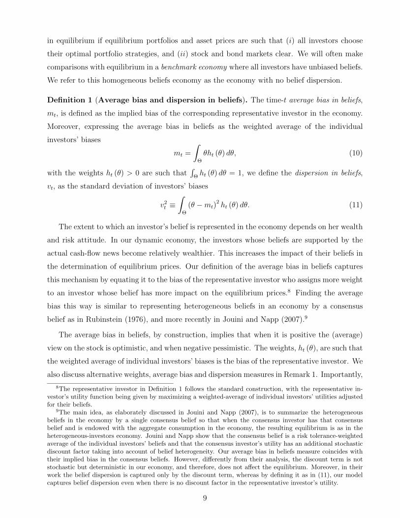
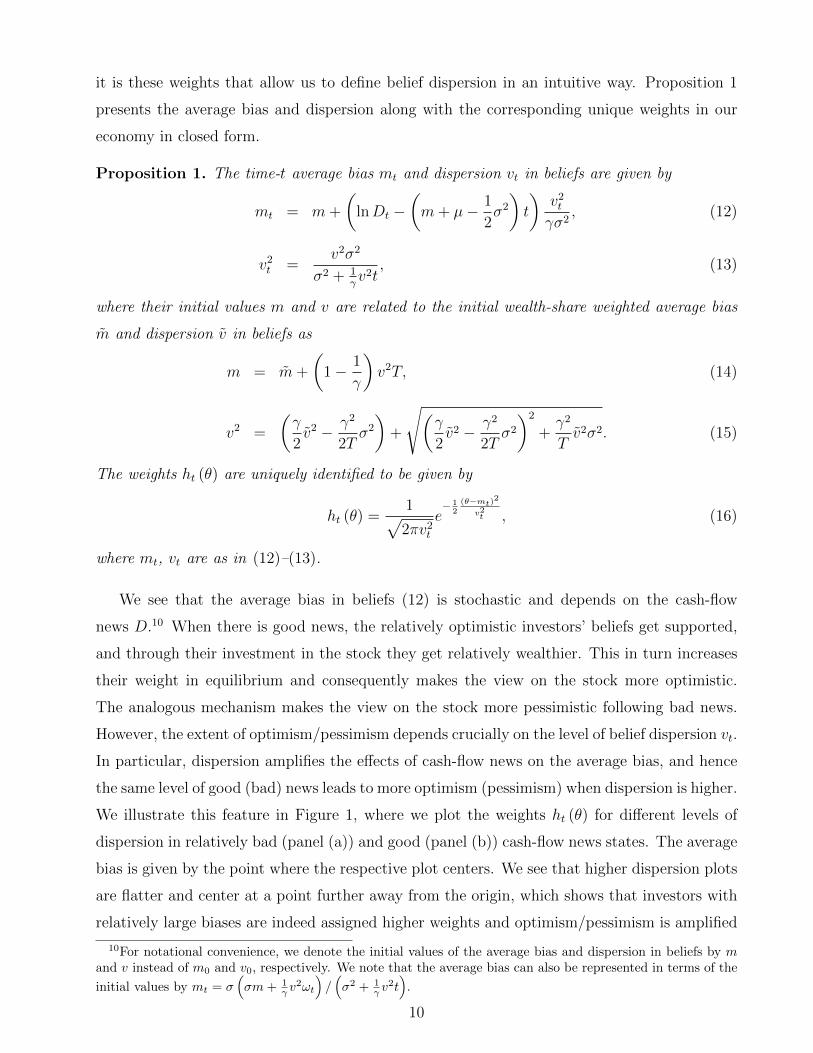
We see that the average bias in beliefs (12) is stochastic and depends on the cash-flow

news D.10 When there is good news, the relatively optimistic investors’ beliefs get supported,

and through their investment in the stock they get relatively wealthier. This in turn increases

their weight in equilibrium and consequently makes the view on the stock more optimistic.

The analogous mechanism makes the view on the stock more pessimistic following bad news.

However, the extent of optimism/pessimism depends crucially on the level of belief dispersion vt.

In particular, dispersion amplifies the effects of cash-flow news on the average bias, and hence

the same level of good (bad) news leads to more optimism (pessimism) when dispersion is higher.

We illustrate this feature in Figure 1, where we plot the weights ht (θ) for different levels of

dispersion in relatively bad (panel (a)) and good (panel (b)) cash-flow news states. The average

bias is given by the point where the respective plot centers. We see that higher dispersion plots

are flatter and center at a point further away from the origin, which shows that investors with

relatively large biases are indeed assigned higher weights and optimism/pessimism is amplified

10For notational convenience, we denote the initial values of the average bias and dispersion in beliefs by mand v instead of m0 and v0, respectively. We note that the average bias can also be represented in terms of the

initial values by mt = σ(σm+ 1

γ v2ωt

)/(σ2 + 1

γ v2t)

.

10

−0.2 −0.15 −0.1 −0.05 0 0.050

5

10

15

Investor type θ

Wei

ghts

vt = 0

vt = 3.2%

vt = 4.2%

(a) Relatively bad news

−0.1 −0.05 0 0.05 0.1 0.150

5

10

15

Investor type θ

Wei

ghts

vt = 0

vt = 3.2%

vt = 4.2%

(b) Relatively good news

Figure 1: Investors’ weights. These panels plot the weights ht (θ) for each distinct θ-type investor

for different levels of current belief dispersion vt. The belief dispersion is vt = 3.2% in solid blue and

4.2% in dashed green lines. The vertical dotted black lines correspond to the benchmark economy with

no belief dispersion. The cash-flow news is relatively bad Dt = 0.5 in panel (a) and good Dt = 1.5in panel (b). The baseline parameter values are: m = 0, v = 3.23%, µ = 9.2%, σ = 11.5%, γ = 1,

t = 0.5 and T = 5.11

under higher dispersion. Investors’ attitude towards risk, γ, influences the average bias too.

As investors become more risk averse, they invest less in the stock and this limits the wealth

transfers in the economy. Consequently, this reduces the sensitivity of the average bias to

cash-flow news, leading to less optimism (pessimism) when the cash-flow news is good (bad).

In the presence of heterogeneity in beliefs, the belief dispersion has a dual role. Besides

amplifying the current average bias in beliefs, the belief dispersion also drives the extent to

which average bias fluctuates over time and hence represents the riskiness of average bias.

Indeed, it can be shown from (12) that the volatility of the average bias in beliefs is σmt = v2t /γσ,

where σmt satisfies dmt = µmtdt + σmtdωt. Hence, the higher the dispersion, the higher the

fluctuations in the average bias, and therefore, the greater the uncertainty investors face. As

11The initial wealth-share weighted average bias in beliefs m is taken to be zero to prevent any effects arisingdue to the initial bias. The initial wealth-share weighted belief dispersion v is chosen to match the time-seriesaverage of the analysts’ forecast dispersion about the earnings growth rate of a market portfolio as reported inYu (2011) for the period (1981-2005) – this yields v = 3.23%. The parameter value for µ, 9.2%, is obtainedby matching it to the realized market excess return in Yu (2011). For σ, we match the initial stock volatility(σS0) given by Propositon 5 to the average market volatility (16%), also reported in Yu (2011). This gives thequadratic equation σ2−σS0σ+ v2T = 0 for σ, which yields the solution as σ = 11.5%. The relative risk aversioncoefficient is set at 1. The current time is set at t = 0.5 and the investment horizon T at 5 years throughoutthe plots. Substituting above parameter values into (13) gives the current belief dispersion as vt = 3.2% afterrounding. To highlight the effects of increased dispersion, we also plot the relevant economic quantities whenthe current belief dispersion is increased to vt = 4.2%.

11

for the dynamics of belief dispersion itself, as (13) highlights, the dispersion is at its highest

level initially and then decreases over time deterministically as investors with extreme beliefs

tend to receive less and less weight over time due to their diminishing wealth and impact in

equilibrium.

Equation (16) indicates that the time-t weights ht (θ), which can be thought of as the time-t

“effective” relative frequency of investors, have a convenient Gaussian form with mean mt and

standard deviation vt as also illustrated in Figure 1. This feature allows us to characterize

the wide range of investor heterogeneity in our economy by the average bias and dispersion

in beliefs since they are the first two (thus sufficient) central moments of Gaussian weights.

Finally, it is worth noting that for logarithmic preferences (γ = 1), the weights coincide with

the wealth-share weights W (θ) /S as discussed in Remark 1.

Remark 1 (Alternative average bias and dispersion in beliefs measures). In heteroge-

neous beliefs models with two agents, the dispersion, or the disagreement, in beliefs is typically

captured by the difference between the biases of the two agents (e.g., Basak (2005), Banerjee

and Kremer (2010), and Xiong and Yan (2010)). With many agents in a dynamic economy,

however, there is no immediately obvious alternative. In our setting, the simplest choice would

be to use the initial distribution of investors as the weights and compute the corresponding

weighted-average bias and dispersion in beliefs. However, this leads to constant average bias

and dispersion measures as in (6)–(7), and so it would not be possible to characterize the

stochastic equilibrium quantities using these constant measures. For a dynamic economy such

as ours, stochastic impact of investors’ beliefs and wealth ought to be taken into account.12

To capture the larger impact of wealthier investors on equilibrium prices, one may use the

wealth-share distribution as the weights. This definition does not require the construction of

the representative investor and yields alternative average bias and dispersion in beliefs measures

denoted by mt and vt, respectively, which can be shown to be given by

mt ≡ˆ

Θ

θWt (θ)

Stdθ = mt −

(1− 1

γ

)v2t (T − t) , (17)

v2t ≡

ˆΘ

(θ − mt)2 Wt (θ)

Stdθ =

1

γv2t +

(1− 1

γ

)v2T , (18)

where mt, vt are as in (12)–(13).13 As equations (17)–(18) highlight, our average bias and

dispersion in beliefs coincide with their respective wealth-share weighted counterparts when the

12This is less of a concern in static models with many agents (e.g., Chen, Hong, and Stein (2002)) since thereare no dynamic belief and wealth transfer considerations.

13Above expressions are proved in the proof of Proposition 5 in Appendix A.

12

preferences are logarithmic (γ = 1) and also at the horizon T . For non-logarithmic preferences,

at any point in time, the wealth-share weighted average bias mt differs from the average bias mt,

but only by a constant. This constant arises since the distinct θ-type investor with the highest

wealth is not the same investor whose bias has the highest impact on equilibrium quantities

when γ 6= 1. However, since the difference between the two average bias measures is a constant,

we obtain similar results and all the predictions of the model remain valid if, instead of mt and

vt, we use the wealth-share weighted average bias and dispersion measures as in (17)–(18).

Following Diether, Malloy, and Scherbina (2002), numerous empirical studies use the stan-

dard deviation of analysts’ earnings forecast levels (normalized by the absolute value of the

mean forecast) as a proxy for investors’ belief dispersion (see footnote 7). In our setting, this

is achieved by considering an alternative belief dispersion measure vt, defined as the standard

deviation of the investors’ subjective expectations about the payoff DT , normalized by the mean

expected payoff. This can be shown to be given by

v2t =

´Θ

(Eθt [DT ]−

´ΘEθt [DT ]ht (θ) dθ

)2ht (θ) dθ´

ΘEθt [DT ]ht (θ) dθ

= ev2t (T−t)2 − 1.

We see that there is a strictly monotonic positive relation between vt and our measure vt, and

therefore, all our implications remain valid under either specification.

4 Stock Price and Mean Return

In this Section, we investigate how the stock price and its mean return are affected by the

average bias and dispersion in beliefs. In particular, we demonstrate that the stock price is

convex in cash-flow news. A higher belief dispersion gives rise to a higher stock price and

a lower mean return when the view on the stock is relatively optimistic, and vice versa when

pessimistic, consistent with empirical evidence. In Section 4.3, we discuss how the more familiar,

otherwise identical heterogeneous beliefs models with two (or finitely many) investors may not

be capable of generating several of our main findings.

4.1 Equilibrium Stock Price

Proposition 2. In the economy with belief dispersion, the equilibrium stock price is given by

St = Stemt(T−t)− 1

2γ(2γ−1)v2t (T−t)2 , (19)

13

where the average bias mt and dispersion vt in beliefs are as in Proposition 1, and the equilibrium

stock price in the benchmark economy with no belief dispersion is given by

St = Dte(µ−γσ2)(T−t). (20)

Consequently, in the presence of belief dispersion,

i) The stock price is higher than in the benchmark economy when mt > (1/2γ) (2γ − 1) v2t (T − t),

and is lower otherwise.

ii) The stock price is convex in cash-flow news Dt.

iii) The stock price is increasing in belief dispersion vt when mt > m+(1/2γ) (2γ − 1) v2t (T − t),

and is decreasing otherwise.

iv) The stock price is decreasing in investors’ risk aversion γ, as in the benchmark economy

for relatively good cash-flow news. However, the stock price is increasing in investors’ risk

aversion for relatively bad cash-flow news and low levels of risk aversion.

The stock price in the benchmark economy is driven by cash-flow news Dt, whereby good

news (higher Dt) leads to a higher stock price since investors increase their expectations of the

stock payoff DT . The equilibrium stock price in the presence of belief dispersion has a simple

structure, and is additionally driven by the average bias mt and dispersion vt in beliefs. The

role of the average bias in beliefs is to increase the stock price further following good news, and

conversely following bad news. This is because, as discussed in Section 3, following good cash-

flow news the view on the stock becomes relatively more optimistic which then leads to a further

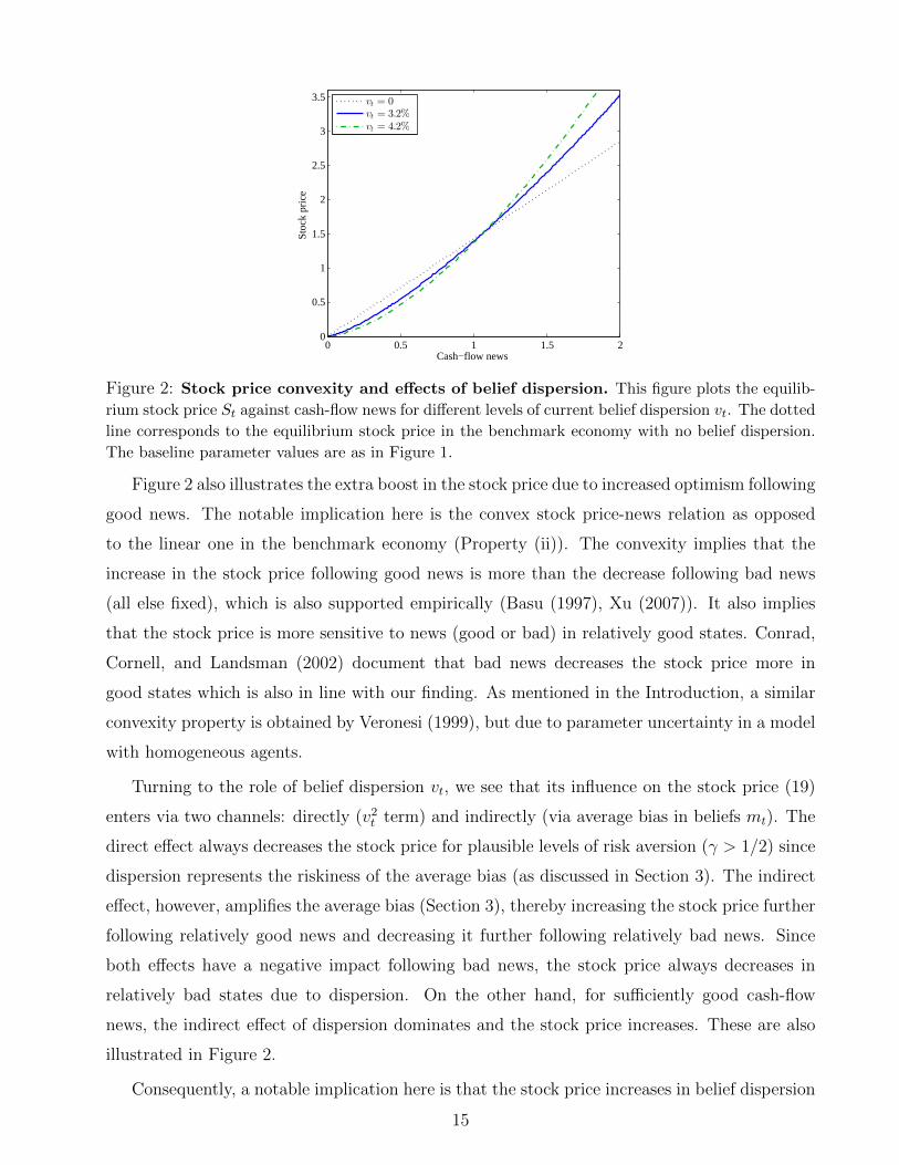
stock price increase, and vice versa following bad news. Figure 2 plots the equilibrium stock

price against cash-flow news for different levels of belief dispersion, illustrating above points.

The stock price being increasing in optimism is consistent with empirical evidence (Brown and

Cliff (2005)), and also implies that the stock price is eventually higher than in the benchmark

economy when the view on the stock is sufficiently optimistic (Property (i)).14 Moreover, this

property implies a feature, against conventional wisdom, that a moderately optimistic view

on the stock can lead to a lower price than in the benchmark economy with unbiased beliefs.

This happens when the negative effect of belief dispersion, as we discuss below, outweighs the

positive effect of optimism.

14For logarithmic preferences (γ = 1), the stock price is higher than in the benchmark economy when mt >(1/2) v2t (T − t). For non-logarithmic preferences, the adjustment for risk aversion generates the (2γ − 1) term.This adjustment is intuitive, since the higher the risk aversion, the more investors dislike the uncertainty in thefuture average bias in beliefs, which is driven by belief dispersion (Section 3), and so the higher the optimismmust be for the stock price to be greater than in the benchmark case.

14

0 0.5 1 1.5 20

0.5

1

1.5

2

2.5

3

3.5

Cash−flow news

Sto

ck p

rice

vt = 0

vt = 3.2%

vt = 4.2%

Figure 2: Stock price convexity and effects of belief dispersion. This figure plots the equilib-

rium stock price St against cash-flow news for different levels of current belief dispersion vt. The dotted

line corresponds to the equilibrium stock price in the benchmark economy with no belief dispersion.

The baseline parameter values are as in Figure 1.

Figure 2 also illustrates the extra boost in the stock price due to increased optimism following

good news. The notable implication here is the convex stock price-news relation as opposed

to the linear one in the benchmark economy (Property (ii)). The convexity implies that the

increase in the stock price following good news is more than the decrease following bad news

(all else fixed), which is also supported empirically (Basu (1997), Xu (2007)). It also implies

that the stock price is more sensitive to news (good or bad) in relatively good states. Conrad,

Cornell, and Landsman (2002) document that bad news decreases the stock price more in

good states which is also in line with our finding. As mentioned in the Introduction, a similar

convexity property is obtained by Veronesi (1999), but due to parameter uncertainty in a model

with homogeneous agents.

Turning to the role of belief dispersion vt, we see that its influence on the stock price (19)

enters via two channels: directly (v2t term) and indirectly (via average bias in beliefs mt). The

direct effect always decreases the stock price for plausible levels of risk aversion (γ > 1/2) since

dispersion represents the riskiness of the average bias (as discussed in Section 3). The indirect

effect, however, amplifies the average bias (Section 3), thereby increasing the stock price further

following relatively good news and decreasing it further following relatively bad news. Since

both effects have a negative impact following bad news, the stock price always decreases in

relatively bad states due to dispersion. On the other hand, for sufficiently good cash-flow

news, the indirect effect of dispersion dominates and the stock price increases. These are also

illustrated in Figure 2.

Consequently, a notable implication here is that the stock price increases in belief dispersion

15

0 2 4 6 8 10

0.4

0.5

0.6

0.7

0.8

Risk aversion γ

Stoc

k pr

ice

v = 0v = 3.23%

v = 4.23%

(a) Relatively bad news

0 2 4 6 8 101.2

1.6

2

2.4

2.8

Risk aversion γ

Stoc

k pr

ice

v = 0v = 3.23%

v = 4.23%

(b) Relatively good news

Figure 3: Effects of risk aversion on stock price. These figures plot the equilibrium stock price

St against relative risk aversion coefficient γ for different levels of initial wealth-share weighted belief

dispersion v. The dotted lines correspond to the equilibrium stock price in the benchmark economy

with no belief dispersion. The cash-flow news is relatively bad Dt = 0.5 in panel (a) and goodDt = 1.5 in panel (b). The baseline parameter values are as in Figure 1.15

when the view on the stock is relatively optimistic, and decreases otherwise (Property (iii)). A

higher belief dispersion leading to a higher stock price is empirically documented by Goetzmann

and Massa (2005) and Yu (2011). This is somewhat surprising since, instead of requiring a

premium for the extra uncertainty due to belief dispersion, investors appear to pay a premium

for it. Our model reconciles with this seemingly counterintuitive finding by demonstrating

that a higher dispersion may lead to a higher stock price when the stock price is driven by

sufficiently optimistic beliefs. This is supported by evidence in Yu (2011). Yu provides evidence

that a higher belief dispersion increases growth stock (low book-to-market) prices more than

value stock prices, and associates growth stocks with optimism motivated by the findings of

Lakonishok, Shleifer, and Vishny (1994), La Porta (1996). He also finds weak evidence that

value stock prices in fact decrease under higher dispersion.

Figure 3 presents the effects of risk aversion on the equilibrium stock price and highlights a

novel finding that the stock price in the presence of belief dispersion may actually increase in

investors’ risk aversion γ (Property (iv)). In the benchmark economy, the stock price always

decreases in investors’ risk aversion. This is intuitive since more risk averse investors demand

15We note that unlike earlier Figures, these plots are not for different levels of current belief dispersion vt butfor different levels of initial wealth-share weighted dispersion v, since vt depends on γ and therefore cannot befixed across different levels of relative risk aversion.

16

a higher return to hold the risky stock and so push down its price. In the presence of belief

dispersion, the risk aversion has an additional impact on the stock price through the average

bias in beliefs. As discussed in Section 3, a higher risk aversion makes the average bias less

sensitive to news since it reduces risk taking and hence the magnitude of wealth transfers among

investors. Therefore, the same level of bad news generates less pessimism and decreases the

stock price less in a more risk averse economy. This creates a range of risk aversion values

for which the stock price actually increases in investors’ risk aversion. On the other hand, for

relatively good news, both the increased risk aversion and the accompanying reduced optimism

induce investors to demand a higher return, which leads to the stock price being monotonically

decreasing in investors’ risk aversion.

Remark 2. The equilibrium stock price in (19) can also be expressed in terms of the volatility

of the average bias in beliefs σmt as

St = Stemt(T−t)− 1

2(2γ−1)σσmt(T−t)2 , (21)

where σmt = v2t /γσ as discussed in Section 3. In Section 6, within a richer setup with Bayesian

learning, we show that the stock price expression is also as is in (21).

4.2 Equilibrium Mean Return

In our economy, the mean return perceived by each θ-type investor, µS (θ), is different than the

(observed) true mean return, µS, with the relation between them being given by (4). To make

our results comparable to empirical studies, in this Section we present our results in terms of

the true mean return (as observed in the data), henceforth, simply referred to as the mean

return. Proposition 3 reports the equilibrium mean return and its properties.

Proposition 3. In the economy with belief dispersion, the equilibrium mean return is given by

µSt = µStv4t

v4T

−mtv2t

v2T

, (22)

where the average bias mt and dispersion vt in beliefs are as in Proposition 1, and the equilibrium

mean return in the benchmark economy with no belief dispersion is given by

µSt = γσ2. (23)

Consequently, in the presence of belief dispersion,

i) The mean return is lower than in the benchmark economy when mt > (v2t + v2

T ) (T − t),

and is higher otherwise.

17

0.4 0.6 0.8 1 1.2 1.4 1.6−0.02

0

0.02

0.04

0.06

0.08

0.1

Cash−flow news

Mea

n re

turn

vt = 0

vt = 3.2%

vt = 4.2%

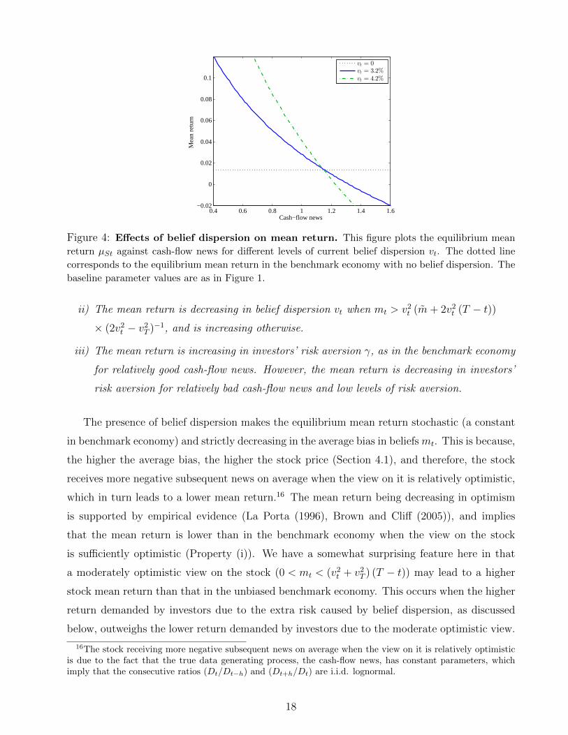
Figure 4: Effects of belief dispersion on mean return. This figure plots the equilibrium mean

return µSt against cash-flow news for different levels of current belief dispersion vt. The dotted line

corresponds to the equilibrium mean return in the benchmark economy with no belief dispersion. The

baseline parameter values are as in Figure 1.

ii) The mean return is decreasing in belief dispersion vt when mt > v2t (m+ 2v2

t (T − t))× (2v2

t − v2T )−1, and is increasing otherwise.

iii) The mean return is increasing in investors’ risk aversion γ, as in the benchmark economy

for relatively good cash-flow news. However, the mean return is decreasing in investors’

risk aversion for relatively bad cash-flow news and low levels of risk aversion.

The presence of belief dispersion makes the equilibrium mean return stochastic (a constant

in benchmark economy) and strictly decreasing in the average bias in beliefs mt. This is because,

the higher the average bias, the higher the stock price (Section 4.1), and therefore, the stock

receives more negative subsequent news on average when the view on it is relatively optimistic,

which in turn leads to a lower mean return.16 The mean return being decreasing in optimism

is supported by empirical evidence (La Porta (1996), Brown and Cliff (2005)), and implies

that the mean return is lower than in the benchmark economy when the view on the stock

is sufficiently optimistic (Property (i)). We have a somewhat surprising feature here in that

a moderately optimistic view on the stock (0 < mt < (v2t + v2

T ) (T − t)) may lead to a higher

stock mean return than that in the unbiased benchmark economy. This occurs when the higher

return demanded by investors due to the extra risk caused by belief dispersion, as discussed

below, outweighs the lower return demanded by investors due to the moderate optimistic view.

16The stock receiving more negative subsequent news on average when the view on it is relatively optimisticis due to the fact that the true data generating process, the cash-flow news, has constant parameters, whichimply that the consecutive ratios (Dt/Dt−h) and (Dt+h/Dt) are i.i.d. lognormal.

18

Figure 4 plots the equilibrium mean return against cash-flow news for different levels of

belief dispersion and illustrates that a higher belief dispersion vt leads to a lower mean return

when the view on the stock is sufficiently optimistic, and to a higher mean return otherwise

(Property (ii)). The intuition for this is similar to that for the stock price: dispersion represents

additional risk for investors (Section 3), and therefore investors demand a higher return to hold

the stock when dispersion is higher. However, we see from (22) that dispersion also multiplies

the average bias in beliefs, which in turn leads to a lower mean return when the view on the

stock is optimistic and to a higher mean return when pessimistic. When there is sufficiently

optimistic view on the stock, the latter effect dominates and produces the negative relation

between belief dispersion and mean return.

As discussed in the Introduction, the empirical evidence on the relation between belief

dispersion and mean return is vast and mixed, and existing theoretical works explain only one

side of this relation. Our model generates both the negative and positive effects and implies that

the documented negative relation must be due to the optimistic bias and it should be stronger,

the higher the optimism. Diether, Malloy, and Scherbina (2002) provide supporting evidence for

our implications by finding an optimistic bias in their study overall, and by also showing that

the negative effect of dispersion is indeed stronger for more optimistic stocks. Similar evidence

is also provided by Yu (2011) who documents that high dispersion stocks earn lower returns

than low dispersion ones and this effect is more pronounced for growth (low book-to-market)

stocks which tend to represent overly optimistic stocks (see, for example, Lakonishok, Shleifer,

and Vishny (1994), La Porta (1996) and Skinner and Sloan (2002)).

Figure 5 plots the equilibrium mean return against investors’ risk aversion γ for different

levels of belief dispersion and highlights an interesting feature that the equilibrium mean return

may decrease in investors’ risk aversion for relatively bad news states over a range of risk aversion

values (Property (iii)). Analogous to the intuition given for the stock price (Section 4.1), this

result is again due to bad news leading to less pessimism in more risk averse economies. We

again note that for relatively good news, the mean return monotonically increases in investors’

risk aversion as in the benchmark economy. This is because both the increased risk aversion

and the accompanying reduced optimism induce investors to demand a higher return.

19

0 2 4 6 8 100

0.04

0.08

0.12

0.16

Risk aversion γ

Mea

n re

turn

v = 0v = 3.23%

v = 4.23%

(a) Relatively bad news

0 2 4 6 8 10

−0.04

0

0.04

0.08

0.12

Risk aversion γ

Mea

n re

turn

v = 0v = 3.23%

v = 4.23%

(b) Relatively good news

Figure 5: Effects of risk aversion on mean return. These figures plot the equilibrium mean return

µSt against relative risk aversion coefficient γ for different levels of initial wealth-share weighted belief

dispersion v. The dotted lines correspond to the equilibrium mean returns in the benchmark economy

with no belief dispersion. The cash-flow news is relatively bad Dt = 0.5 in panel (a) and goodDt = 1.5 in panel (b). For the choice of dispersion parameter values see footnote 15. The baseline

parameter values are as in Figure 1.

4.3 Comparisons with Two-Investor Economy

In our economy, investor heterogeneity does not vary across states of the world (since belief

dispersion vt is deterministic), and hence does not vanish in relatively extreme states. However,

this is not the case for otherwise identical heterogeneous beliefs models with two (or finitely

many) investors having CRRA preferences over horizon wealth.17 In these models, the (most)

pessimistic investor would control almost all the wealth in the economy in very bad news

states, while the (most) optimistic investor would hold all wealth in very good news states.

This vanishes the effective investor heterogeneity in such states and forces the model to have

implications similar to those in a single investor economy, which then yields irregular behavior

for economic quantities across states of the world.

To better highlight the effects of vanishing effective heterogeneity, Figure 6 plots the equilib-

rium stock price and mean return against cash-flow news in an otherwise identical two-investor

economy, with one investor being optimistic and the other pessimistic. The equilibrium ex-

pressions are provided in Appendix A.2 and are for logarithmic preferences to be consistent

17Without loss of generality, we consider the more familiar two-investor economy, Θ = {θ1, θ2}, in our dis-cussion here. However, the arguments and the plots presented here are valid for the more general otherwiseidentical heterogeneous beliefs models with finitely many investors, Θ = {θ1, . . . , θN}, as discussed in AppendixA.2. Examples of other works using this economic setup include Kogan, Ross, Wang, and Westerfield (2006)(two investors) and Cvitanic and Malamud (2011) (finitely many investors).

20

0 0.5 1 1.5 20

0.5

1

1.5

2

2.5

3

3.5

Cash−flow news

Sto

ck p

rice

Spt

Sopt

Sot

(a) Stock price

0 0.5 1 1.5 2

−0.04

−0.02

0

0.02

0.04

0.06

0.08

Cash−flow news

Mea

n re

turn

µp

St

µop

St

µoSt

(b) Mean return

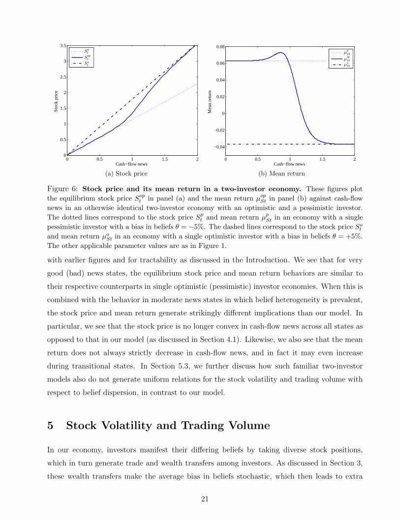
Figure 6: Stock price and its mean return in a two-investor economy. These figures plot

the equilibrium stock price Sopt in panel (a) and the mean return µopSt in panel (b) against cash-flow

news in an otherwise identical two-investor economy with an optimistic and a pessimistic investor.

The dotted lines correspond to the stock price Spt and mean return µpSt in an economy with a single

pessimistic investor with a bias in beliefs θ = −5%. The dashed lines correspond to the stock price Sotand mean return µoSt in an economy with a single optimistic investor with a bias in beliefs θ = +5%.

The other applicable parameter values are as in Figure 1.

with earlier figures and for tractability as discussed in the Introduction. We see that for very

good (bad) news states, the equilibrium stock price and mean return behaviors are similar to

their respective counterparts in single optimistic (pessimistic) investor economies. When this is

combined with the behavior in moderate news states in which belief heterogeneity is prevalent,

the stock price and mean return generate strikingly different implications than our model. In

particular, we see that the stock price is no longer convex in cash-flow news across all states as

opposed to that in our model (as discussed in Section 4.1). Likewise, we also see that the mean

return does not always strictly decrease in cash-flow news, and in fact it may even increase

during transitional states. In Section 5.3, we further discuss how such familiar two-investor

models also do not generate uniform relations for the stock volatility and trading volume with

respect to belief dispersion, in contrast to our model.

5 Stock Volatility and Trading Volume

In our economy, investors manifest their differing beliefs by taking diverse stock positions,

which in turn generate trade and wealth transfers among investors. As discussed in Section 3,

these wealth transfers make the average bias in beliefs stochastic, which then leads to extra

21

uncertainty for investors. In this Section, we demonstrate how this extra uncertainty and

investors’ trading motives give rise to excess stock volatility and trading volume. We further

show that a higher belief dispersion leads to a higher stock volatility and trading volume in

our model. These findings are well supported by empirical evidence. However, in Section 5.3

(analogously to Section 4.3), we show that a higher belief dispersion has ambiguous effects on

the stock volatility and trading volume in the more familiar, otherwise identical heterogeneous

beliefs models with two (or finitely many) investors.

5.1 Equilibrium Stock Volatility

Proposition 4. In the economy with belief dispersion, the equilibrium stock volatility is given

by

σSt = σSt +v2t

γσ(T − t) , (24)

where the dispersion in beliefs vt is as in Proposition 1, and the equilibrium stock volatility in

the benchmark economy with no belief dispersion is given by

σSt = σ. (25)

Consequently, in the presence of belief dispersion,

i) The stock volatility is higher than in the benchmark economy.

ii) The stock volatility is increasing in belief dispersion vt.

iii) The stock volatility is decreasing in investors’ risk aversion γ.

The key implication of Proposition 4 is that the belief dispersion vt generates excess volatility

in our economy by amplifying the stock volatility beyond the fundamental payoff uncertainty

σ.18 This is because, as discussed in Section 4, the stock price increases more than in the

benchmark economy following good cash-flow news and decreases more following bad cash-flow

news. This additional fluctuation in the stock price across news states generates the excess

stock volatility (Property (i)). This is consistent with the well-documented empirical evidence

that stock volatilities are too high to be justified by fundamental uncertainty (Leroy and Porter

(1981), Shiller (1981)).

Naturally, the higher the belief dispersion, the higher the excess stock volatility (Property

(ii)). This is because when dispersion is higher, the average bias in beliefs fluctuates more

18The stock volatility can also be written as σSt = σStv2t /v

2T where the ratio v2t /v

2T > 1 for all t < T .

22

0 0.01 0.02 0.03 0.04 0.050.1

0.12

0.14

0.16

0.18

0.2

0.22

Belief dispersion

Stoc

k vo

latil

ity

σSt

σSt

(a) Effects of belief dispersion

0 2 4 6 8 100.1

0.12

0.14

0.16

0.18

0.2

0.22

Risk aversion γ

Stoc

k vo

latil

ity

v = 0v = 3.23%

v = 4.23%

(b) Effects of risk aversion

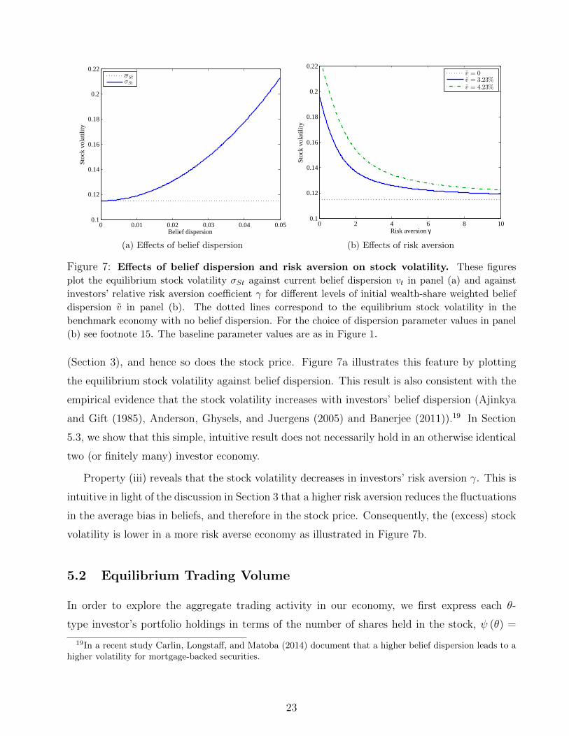
Figure 7: Effects of belief dispersion and risk aversion on stock volatility. These figures

plot the equilibrium stock volatility σSt against current belief dispersion vt in panel (a) and against

investors’ relative risk aversion coefficient γ for different levels of initial wealth-share weighted belief

dispersion v in panel (b). The dotted lines correspond to the equilibrium stock volatility in the

benchmark economy with no belief dispersion. For the choice of dispersion parameter values in panel

(b) see footnote 15. The baseline parameter values are as in Figure 1.

(Section 3), and hence so does the stock price. Figure 7a illustrates this feature by plotting

the equilibrium stock volatility against belief dispersion. This result is also consistent with the

empirical evidence that the stock volatility increases with investors’ belief dispersion (Ajinkya

and Gift (1985), Anderson, Ghysels, and Juergens (2005) and Banerjee (2011)).19 In Section

5.3, we show that this simple, intuitive result does not necessarily hold in an otherwise identical

two (or finitely many) investor economy.

Property (iii) reveals that the stock volatility decreases in investors’ risk aversion γ. This is

intuitive in light of the discussion in Section 3 that a higher risk aversion reduces the fluctuations

in the average bias in beliefs, and therefore in the stock price. Consequently, the (excess) stock

volatility is lower in a more risk averse economy as illustrated in Figure 7b.

5.2 Equilibrium Trading Volume

In order to explore the aggregate trading activity in our economy, we first express each θ-

type investor’s portfolio holdings in terms of the number of shares held in the stock, ψ (θ) =

19In a recent study Carlin, Longstaff, and Matoba (2014) document that a higher belief dispersion leads to ahigher volatility for mortgage-backed securities.

23

0 0.05 0.1 0.15 0.20

0.2

0.4

0.6

0.8

Belief dispersion

Tra

ding

vol

ume

mea

sure

γ=1

γ=3

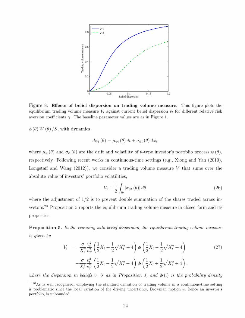
Figure 8: Effects of belief dispersion on trading volume measure. This figure plots the

equilibrium trading volume measure Vt against current belief dispersion vt for different relative risk

aversion coefficients γ. The baseline parameter values are as in Figure 1.

φ (θ)W (θ) /S, with dynamics

dψt (θ) = µψt (θ) dt+ σψt (θ) dωt,

where µψ (θ) and σψ (θ) are the drift and volatility of θ-type investor’s portfolio process ψ (θ),

respectively. Following recent works in continuous-time settings (e.g., Xiong and Yan (2010),

Longstaff and Wang (2012)), we consider a trading volume measure V that sums over the

absolute value of investors’ portfolio volatilities,

Vt ≡1

2

ˆΘ

|σψt (θ)| dθ, (26)

where the adjustment of 1/2 is to prevent double summation of the shares traded across in-

vestors.20 Proposition 5 reports the equilibrium trading volume measure in closed form and its

properties.

Proposition 5. In the economy with belief dispersion, the equilibrium trading volume measure

is given by

Vt =σ

X2t

v2t

v2T

(1

2Xt +

1

2

√X2t + 4

)φ

(1

2Xt −

1

2

√X2t + 4

)(27)

− σ

X2t

v2t

v2T

(1

2Xt −

1

2

√X2t + 4

)φ

(1

2Xt +

1

2

√X2t + 4

),

where the dispersion in beliefs vt is as in Proposition 1, and φ (.) is the probability density

20As is well recognized, employing the standard definition of trading volume in a continuous-time settingis problematic since the local variation of the driving uncertainty, Brownian motion ω, hence an investor’sportfolio, is unbounded.

24

function of the standard normal random variable, and X is a (positive) deterministic process

given by

X2t = γ2σ

4

v4T

[1

γv2t +

(1− 1

γ

)v2T

].

Consequently, in the presence of belief dispersion,

i) The trading volume measure is increasing in belief dispersion vt.

ii) The trading volume measure is positively related to the stock volatility σSt.

iii) The trading volume measure is decreasing in investors’ risk aversion γ.

With belief dispersion, investors take diverse stock positions following cash-flow news, which

in turn generate non-trivial trading activity. Naturally, the aggregate trading activity in the

stock, which is captured by our trading volume measure V, increases as the belief dispersion

increases (Property (i)). This is because, when dispersion is higher, investors with relatively

different beliefs have more weight and higher trading demand, which increase the stock trading

volume. Figure 8 illustrates this feature by depicting the equilibrium trading volume measure

against belief dispersion. This result is well-supported by empirical evidence (Ajinkya, Atiase,

and Gift (1991), Bessembinder, Chan, and Seguin (1996) and Goetzmann and Massa (2005)).

We again note that this simple, intuitive result does not necessarily hold in an otherwise identical

two (or finitely many) investor economies as discussed in Section 5.3.

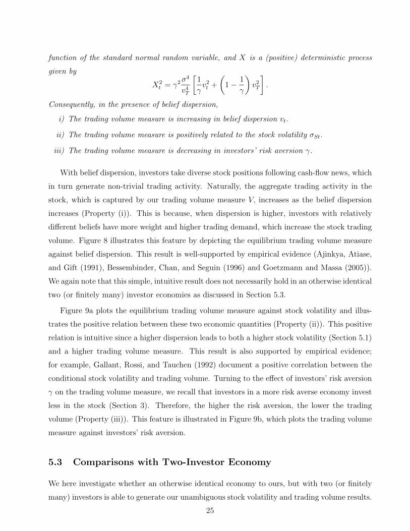
Figure 9a plots the equilibrium trading volume measure against stock volatility and illus-

trates the positive relation between these two economic quantities (Property (ii)). This positive

relation is intuitive since a higher dispersion leads to both a higher stock volatility (Section 5.1)

and a higher trading volume measure. This result is also supported by empirical evidence;

for example, Gallant, Rossi, and Tauchen (1992) document a positive correlation between the

conditional stock volatility and trading volume. Turning to the effect of investors’ risk aversion

γ on the trading volume measure, we recall that investors in a more risk averse economy invest

less in the stock (Section 3). Therefore, the higher the risk aversion, the lower the trading

volume (Property (iii)). This feature is illustrated in Figure 9b, which plots the trading volume

measure against investors’ risk aversion.

5.3 Comparisons with Two-Investor Economy

We here investigate whether an otherwise identical economy to ours, but with two (or finitely

many) investors is able to generate our unambiguous stock volatility and trading volume results.

25

0.1 0.15 0.2 0.250

0.1

0.2

0.3

0.4

0.5

Stock volatility

Trad

ing

volu

me

mes

ure

γ=1

γ=3

(a) Trading volume-stock volatility relation

0 2 4 6 8 10

0

0.1

0.2

0.3

0.4

0.5

Risk aversion γ

Tra

ding

vol

ume

mea

sure

v = 3.23%

v = 4.23%

(b) Effects of risk aversion

Figure 9: Trading volume-stock volatility relation and effects of risk aversion. These figures

plot the equilibrium trading volume measure Vt against stock volatility σSt in panel (a) and against

investors’ relative risk aversion coefficient γ for different levels of initial wealth-share weighted belief

dispersion v in panel (b). For the choice of dispersion parameter values in panel (b) see footnote 15.

The baseline parameter values are as in Figure 1.

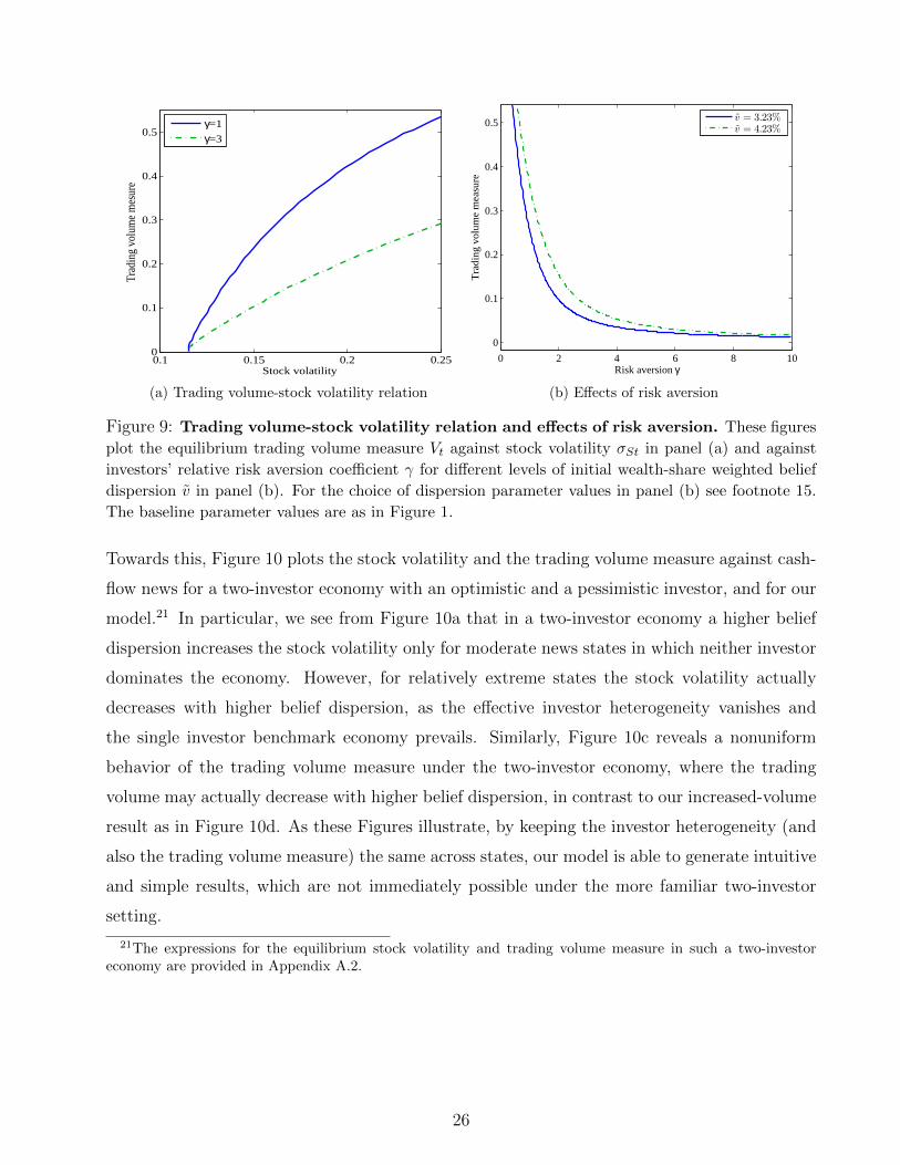
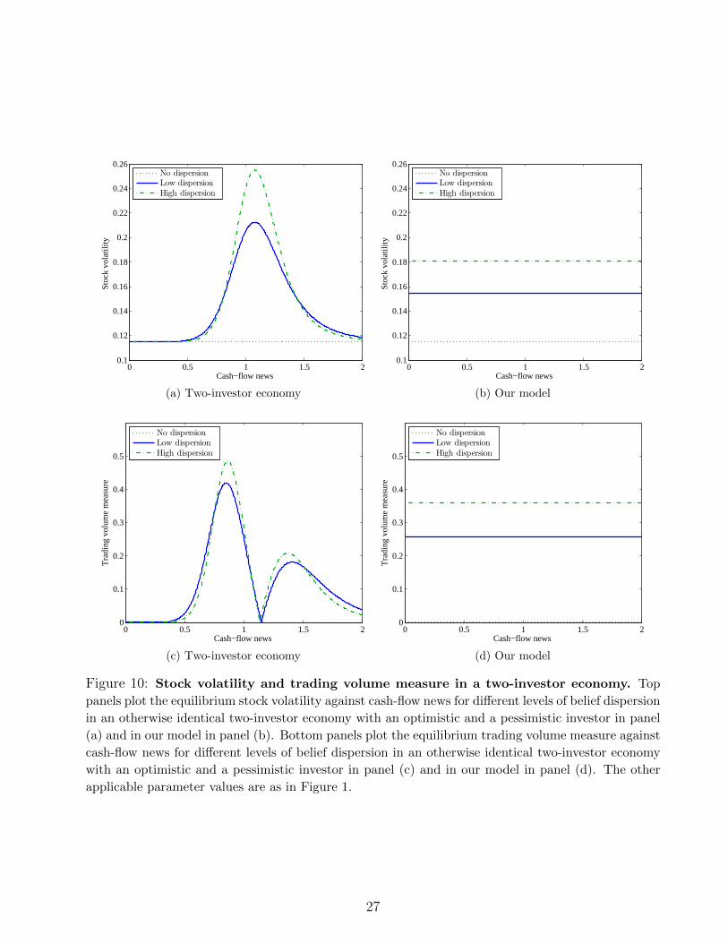
Towards this, Figure 10 plots the stock volatility and the trading volume measure against cash-

flow news for a two-investor economy with an optimistic and a pessimistic investor, and for our

model.21 In particular, we see from Figure 10a that in a two-investor economy a higher belief

dispersion increases the stock volatility only for moderate news states in which neither investor

dominates the economy. However, for relatively extreme states the stock volatility actually

decreases with higher belief dispersion, as the effective investor heterogeneity vanishes and

the single investor benchmark economy prevails. Similarly, Figure 10c reveals a nonuniform

behavior of the trading volume measure under the two-investor economy, where the trading

volume may actually decrease with higher belief dispersion, in contrast to our increased-volume

result as in Figure 10d. As these Figures illustrate, by keeping the investor heterogeneity (and

also the trading volume measure) the same across states, our model is able to generate intuitive

and simple results, which are not immediately possible under the more familiar two-investor

setting.

21The expressions for the equilibrium stock volatility and trading volume measure in such a two-investoreconomy are provided in Appendix A.2.

26

0 0.5 1 1.5 20.1

0.12

0.14

0.16

0.18

0.2

0.22

0.24

0.26

Cash−flow news

Sto

ck v

olat

ility

No dispersion

Low dispersion

High dispersion

(a) Two-investor economy

0 0.5 1 1.5 20.1

0.12

0.14

0.16

0.18

0.2

0.22

0.24

0.26

Cash−flow news S

tock

vol

atili

ty

No dispersion

Low dispersion

High dispersion

(b) Our model

0 0.5 1 1.5 20

0.1

0.2

0.3

0.4

0.5

Cash−flow news

Tra

ding

vol

ume

mea

sure

No dispersion

Low dispersion

High dispersion

(c) Two-investor economy

0 0.5 1 1.5 20

0.1

0.2

0.3

0.4

0.5

Cash−flow news

Tra

ding

vol

ume

mea

sure

No dispersion

Low dispersion

High dispersion

(d) Our model

Figure 10: Stock volatility and trading volume measure in a two-investor economy. Top

panels plot the equilibrium stock volatility against cash-flow news for different levels of belief dispersion

in an otherwise identical two-investor economy with an optimistic and a pessimistic investor in panel

(a) and in our model in panel (b). Bottom panels plot the equilibrium trading volume measure against

cash-flow news for different levels of belief dispersion in an otherwise identical two-investor economy

with an optimistic and a pessimistic investor in panel (c) and in our model in panel (d). The other

applicable parameter values are as in Figure 1.

27

6 Economy with Bayesian Learning

So far, we have studied an economy where investors have dogmatic beliefs, which not only

simplified the analysis, but also demonstrated that our results are not driven by investors’

learning. In this Section, we consider a setting with parameter uncertainty and more rational

behavior for investors who optimally update their beliefs in a Bayesian fashion over time as

more data becomes available. This setting is also tractable. We again obtain fully-closed form

solutions for all quantities of interest, and show that all our results remain valid in this richer,

incomplete information economy. This specification also enables us disentangle the effects of

belief dispersion and parameter uncertainty on excess volatility, and establish the result that

the investors’ Bayesian learning induces less excess volatility when belief dispersion is higher.

To incorporate Bayesian learning, we make the following modification to investors’ beliefs.

The investors are again indexed by their type θ, but instead of believing the mean growth rate

of the expected payoff is µ+θ at all times 0 ≤ t ≤ T , now the θ-type investor at time 0 believes

that the mean growth rate of the expected payoff is normally distributed with mean µ+ θ and

variance s2, N (µ+ θ, s2). This allows us to interpret a θ-type investor as an investor with an

initial bias of θ in her beliefs. The identical prior variance s2 for all investors ensures that our

results are not driven by heterogeneity in confidence of their estimates. The normal prior and

the Bayesian updating rule imply that the time-t posterior distribution of µ, conditional on the

information set Ft = {Ds : 0 ≤ s ≤ t}, is also normally distributed, N (µ + θt, s2t ), where the

time-t bias of θ-type investor θt (difference between her mean estimate and the true µ) and the

type-independent mean squared error s2t , which represents the level of parameter uncertainty,

are reported in Proposition 6. Therefore, under the θ-type investor’s beliefs, the posterior

cash-flow news process has dynamics

dDt = Dt[(µ+ θt)dt+ σdωt (θ)],

where ω (θ) is her perceived Brownian motion with respect to her own probability measure Pθ,

and is given by dωt (θ) = dωt− (θt/σ)dt. We note that this specification conveniently nests the

earlier dogmatic beliefs economy when s2 = 0.

6.1 Equilibrium in the Presence of Bayesian Learning

We construct the average bias and dispersion in beliefs following Definition 1 in Section 3:

the time-t average bias in beliefs, mt, is the implied bias of the corresponding representative

28

investor, expressed as the weighted average of the individual investors’ biases

mt =

ˆΘ

θtht (θ) dθ, (28)

with the weights ht (θ) > 0 are such that´

Θht (θ) dθ = 1, while the dispersion in beliefs, vt, is

the standard deviation of investors’ biases

v2t ≡ˆ

Θ

(θt −mt)2ht (θ) dθ. (29)

Proposition 6 reports the average bias and dispersion in beliefs along with the corresponding

unique weights in this economy with belief dispersion and parameter uncertainty in closed form.

Proposition 6. The time-t average bias mt and dispersion vt in beliefs are given by

mt = m+

(lnDt −

(m+ µ− 1

2σ2

)t

)(1

γv2 + s2

)1

σ2

v2t

v2

s2

s2t

, (30)

v2t =

v2σ2

σ2 +(

1γv2 + s2

)t

s2t

s2, (31)

where the investors’ time-t parameter uncertainty st is given by

s2t =

s2σ2

σ2 + s2t, (32)

and the initial values m and v are related to the initial wealth-share weighted average bias m

and dispersion v in beliefs as

m = m+

(1− 1

γ

)v2T, (33)

v2 =

(γ

2v2 − γ2

2T

(σ2 + s2T

))+

√(γ

2v2 − γ2

2T(σ2 + s2T )

)2

+γ2

Tv2 (σ2 + s2T ). (34)

The weights ht (θ) are uniquely identified to be given by

ht (θ) =1√2πv2

t

e− 1

2

(θt−mt)2

v2ts2t

s2, (35)

where mt, vt and st are as in (30)–(32) and the time-t bias of θ-type investor θt is given by

θt =s2t

s2θ +

s2t

σωt. (36)

Consequently, in the presence of belief dispersion and parameter uncertainty, for economies with

the same initial average bias m and dispersion v,

i) The average bias in beliefs is increasing in parameter uncertainty st when

Dt > exp((m+ µ− 1

2σ2)t), and is decreasing otherwise.

ii) The dispersion in beliefs is decreasing in parameter uncertainty st.

29

The average bias and dispersion in beliefs (30)–(31) are generalizations of the earlier dog-

matic beliefs case and are now additionally driven by parameter uncertainty st.22 We see that,

similarly to the effect of dispersion, a higher parameter uncertainty leads to a relatively more

optimistic (pessimistic) view on the stock following good (bad) news (Property (i)), and this

then amplifies the volatility of the average bias relative to the dogmatic beliefs case. However,

the underlying mechanisms of belief dispersion and parameter uncertainty are notably differ-

ent. In the case of dispersion, the view on the stock becomes more optimistic following good

news, because the optimistic investors, whose beliefs are supported, become wealthier and this

increases their impact on the average bias in beliefs. In the case of parameter uncertainty, the

view on the stock becomes more optimistic following good news, because all Bayesian investors

increase their estimates of the mean growth rate of the expected payoff µ. Proposition 6 also

reveals that a higher parameter uncertainty leads to a lower dispersion in beliefs (Property (ii)).

This is intuitive because investors’ estimates of µ is a weighted average of their prior and the

data (cash-flow news). The higher the parameter uncertainty, the more weight investors place

on the data, which in turn reduces the differences in their estimates and the belief dispersion.

We remark that in this Section, we consider the effects of parameter uncertainty st only for

economies with the same initial average bias m and dispersion v, as highlighted in Proposition

6. This way, economies only differ in their initial level of parameter uncertainty s and our

results are not driven by the indirect effects through the initial average bias and dispersion.23

6.2 Equilibrium Stock Price and Mean Return

Proposition 7. In the economy with belief dispersion and parameter uncertainty, the equilib-

rium stock price and mean return are given by

St = Stemt(T−t)− 1

2(2γ−1)( 1

γv2+s2) v

2tv2

s2

s2t(T−t)2

, (37)

µSt = µStv4t

v4T

s4T

s4t

−mtv2t

v2T

s2T

s2t

, (38)

22Note that when s2 = 0, the ratio s2t/s2 = 1 for all t, and the expressions in Proposition 6 collapse down to

the dogmatic beliefs economy expressions in Proposition 1.23This is established by letting the initial indirect effect of parameter uncertainty fall on the initial wealth-

share weighted average bias m and dispersion in beliefs v, using the monotonic relations between m and m, andv and v

m = m−(

1− 1

γ

)v2T, v2 = v2

(σ2 + s2T

)+ 1

γ2 v2T

(σ2 + s2T ) + 1γ v

2T.

For the effects of belief dispersion vt and investors risk aversion γ, comparing economies with the same initialaverage bias m and dispersion v is not necessary, as in our earlier analysis with dogmatic beliefs, since let-ting these effects fall on either the initial average bias m and dispersion v, or on their wealth-share weightedcounterparts, yields similar results.

30

where the average bias mt, dispersion vt in beliefs and parameter uncertainty st are as in

Proposition 6 and the equilibrium stock price St and mean return µSt in the benchmark economy

with no belief dispersion are as in Propositions 2–3, respectively.

Consequently, in the presence of belief dispersion and parameter uncertainty, in addition to

the properties in Propositions 2–3, for economies with the same initial average bias m and

dispersion v,

i) The stock price is increasing in parameter uncertainty st when

mt > m+ (1/2) (2γ − 1) ((v2/γ) + s2) (v2t s

2/v2s2t ) (T − t), and is decreasing otherwise.

ii) The mean return is decreasing in parameter uncertainty st when

mt > [m+ 2γσ2 ((v2t s

2T/v

2T s

2t )− 1)] [2− (v2

T s2t/v

2t s

2T )]−1

, and is increasing otherwise.

Proposition 7 confirms that our earlier implications for the stock price and mean return

remain valid with Bayesian learning. However, the stock price and mean return are now also

driven by the parameter uncertainty st. Similarly to the effects of belief dispersion, the stock

price increases while its mean return decreases in parameter uncertainty when the view on

the stock is sufficiently optimistic, and vice versa when pessimistic (Properties (i)–(ii)). More

notably, the additional effect due to the investors’ learning now makes the stock price more

convex as compared with the dogmatic beliefs case. These effects are illustrated in Figure 11

which depicts the equilibrium stock price and mean return against the cash-flow news. The

empirical evidence on the effects of parameter uncertainty on asset prices are limited. Massa

and Simonov (2005) show that both the investors’ learning and the dispersion in beliefs are

conditionally priced, whereas Ozoguz (2009) provides evidence that parameter uncertainty has

a negative impact on the stock price in bad times, which is consistent with our finding.

6.3 Equilibrium Stock Volatility and Trading Volume

Proposition 8. In the economy with belief dispersion and parameter uncertainty, the equilib-

rium stock volatility and the trading volume measure are given by

σSt = σSt +1

σ

(1

γv2 + s2

)v2t

v2

s2

s2t

(T − t) , (39)

Vt =σ

X2t

v2t

v2T

s2T

s2t

(1

2Xt +

1

2

√X2t + 4

)φ

(1

2Xt −

1

2

√X2t + 4

)(40)

− σ

X2t

v2t

v2T

s2T

s2t

(1

2Xt −

1

2

√X2t + 4

)φ

(1

2Xt +

1

2

√X2t + 4

),

31

0 0.5 1 1.5 20

0.5

1

1.5

2

2.5

3

3.5

Cash−flow news

Sto

ck p

rice

vt = st = 0

vt = 3.2%; st = 0

vt =3.14%; st =1.49%

(a) Stock price

0.4 0.6 0.8 1 1.2 1.4 1.6−0.02

0

0.02

0.04

0.06

0.08

0.1

Cash−flow news

Mea

n re

turn

vt = st = 0

vt = 3.2%; st = 0

vt =3.14%; st =1.49%

(b) Stock mean return

Figure 11: Effects of parameter uncertainty on stock price and mean return. These figures

plot the equilibrium stock price St in panel (a) and mean return µSt in panel (b) against cash-flow

news. The dotted black (solid blue) lines correspond to the equilibrium stock price and mean returns

in the benchmark economy with no belief dispersion (economy with belief dispersion and no parameter

uncertainty). The dashdot red lines correspond to the equilibrium stock price and mean returns in

the economy with belief dispersion and parameter uncertainty. The baseline parameter values are as

in Figure 1.24

where the dispersion in beliefs vt and the parameter uncertainty st are as in Proposition 6, and

the equilibrium stock volatility σSt in the benchmark economy with no belief dispersion is as

in Proposition 4, and φ (.) is the probability density function of the standard normal random

variable, and X is a (positive) deterministic process given by

X2t =

γ2σ4

v4T

[1

γv2t

s4T

s4t

+

(1− 1

γ

)v2T

]. (41)

Consequently, in the presence of belief dispersion and parameter uncertainty, in addition to

the properties in Propositions 4–5, for economies with the same initial average bias m and

dispersion v,

i) The stock volatility is increasing in parameter uncertainty st.

ii) The effect of parameter uncertainty st on stock volatility is decreasing in belief dispersion

vt.

iii) The trading volume measure is decreasing in parameter uncertainty st when investors’

risk aversion γ ≥ 1, and it may increase or decrease otherwise.

24The initial belief dispersion v is set as v = 3.23% as in Figure 1. However, due to Bayesian learning, thetime-t dispersion now becomes vt = 3.14% instead of vt = 3.20%. The parameter value for s is obtained by

32

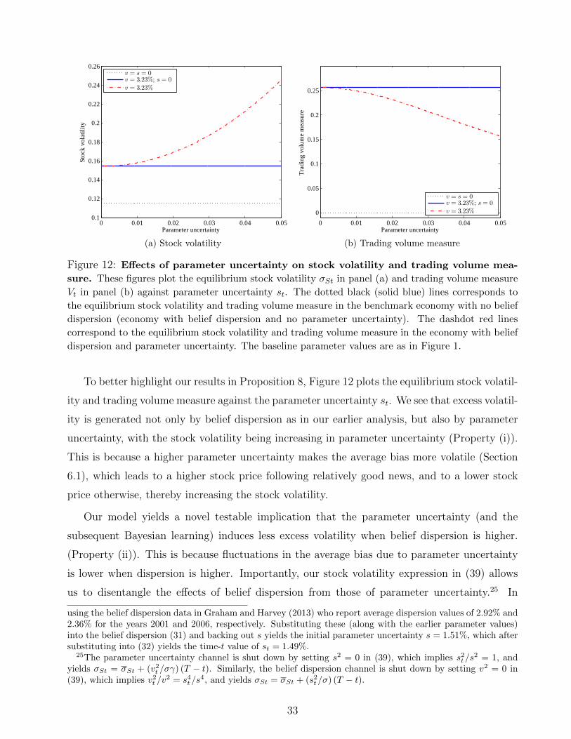
0 0.01 0.02 0.03 0.04 0.050.1

0.12

0.14

0.16

0.18

0.2

0.22

0.24

0.26

Parameter uncertainty

Stoc

k vo

latil

ity

v = s = 0v = 3.23%; s = 0

v = 3.23%

(a) Stock volatility

0 0.01 0.02 0.03 0.04 0.05

0

0.05

0.1

0.15

0.2

0.25

Parameter uncertainty

Tra

ding

vol

ume

mea

sure

v = s = 0v = 3.23%; s = 0

v = 3.23%

(b) Trading volume measure

Figure 12: Effects of parameter uncertainty on stock volatility and trading volume mea-

sure. These figures plot the equilibrium stock volatility σSt in panel (a) and trading volume measure

Vt in panel (b) against parameter uncertainty st. The dotted black (solid blue) lines corresponds to

the equilibrium stock volatility and trading volume measure in the benchmark economy with no belief

dispersion (economy with belief dispersion and no parameter uncertainty). The dashdot red lines

correspond to the equilibrium stock volatility and trading volume measure in the economy with belief

dispersion and parameter uncertainty. The baseline parameter values are as in Figure 1.

To better highlight our results in Proposition 8, Figure 12 plots the equilibrium stock volatil-

ity and trading volume measure against the parameter uncertainty st. We see that excess volatil-

ity is generated not only by belief dispersion as in our earlier analysis, but also by parameter

uncertainty, with the stock volatility being increasing in parameter uncertainty (Property (i)).

This is because a higher parameter uncertainty makes the average bias more volatile (Section

6.1), which leads to a higher stock price following relatively good news, and to a lower stock

price otherwise, thereby increasing the stock volatility.

Our model yields a novel testable implication that the parameter uncertainty (and the

subsequent Bayesian learning) induces less excess volatility when belief dispersion is higher.

(Property (ii)). This is because fluctuations in the average bias due to parameter uncertainty

is lower when dispersion is higher. Importantly, our stock volatility expression in (39) allows

us to disentangle the effects of belief dispersion from those of parameter uncertainty.25 In

using the belief dispersion data in Graham and Harvey (2013) who report average dispersion values of 2.92% and2.36% for the years 2001 and 2006, respectively. Substituting these (along with the earlier parameter values)into the belief dispersion (31) and backing out s yields the initial parameter uncertainty s = 1.51%, which aftersubstituting into (32) yields the time-t value of st = 1.49%.

25The parameter uncertainty channel is shut down by setting s2 = 0 in (39), which implies s2t/s2 = 1, and

yields σSt = σSt + (v2t /σγ) (T − t). Similarly, the belief dispersion channel is shut down by setting v2 = 0 in(39), which implies v2t /v

2 = s4t/s4, and yields σSt = σSt + (s2t/σ) (T − t).

33

the literature, both channels are proposed to explain the excess stock volatility, among other

channels. Barsky and De Long (1993), Timmermann (1993, 1996) show that the excess volatility

in the stock market is broadly consistent with models in which investors are uncertain about

parameters and estimate them from observable processes. We discussed the belief dispersion

channel in Section 5. By disentangling these effects, our result may help future works to

measure the relative contributions of parameter uncertainty and belief dispersion in excess

volatility better.

Finally, we find that the trading volume measure decreases in parameter uncertainty st for

plausible levels of risk aversion γ ≥ 1 (Property (iii)). This is illustrated in Figure 12b and

happens because a higher parameter uncertainty leads to a lower belief dispersion (Section 6.1),

and if there are no opposing effects, as in the case of γ ≥ 1, the lower dispersion unambiguously

decreases the trading volume as in our earlier analysis. For γ < 1, there is an opposing

effect coming from the wealth-share weighted dispersion (ratio v2t /vt may increase in parameter

uncertainty) in addition to the effect of lower dispersion. When this effect is significant, the

trading volume measure may increase in parameter uncertainty.

7 Conclusion

In this paper, we have developed a dynamic model of belief dispersion which simultaneously

explains the empirical regularities in a stock price, its mean return, volatility, and trading

volume. In our analysis, we have determined two sufficient measures, the average bias and

dispersion in beliefs, to summarize the wide range of investors’ beliefs and have demonstrated

that the equilibrium quantities are driven by these two key variables. Our model is tractable

and delivers exact closed-form expressions for all quantities, implying the following. We have

found that the stock price increases in cash-flow news in a convex manner. We have also

shown that the stock price increases and its mean return decreases in belief dispersion when

the view on the stock is optimistic, and vice versa when pessimistic. We have found that the

presence of belief dispersion produces excess stock volatility, trading volume, and a positive

relation between these two quantities. Furthermore, we have disentangled the effects of belief

dispersion from the effects of learning, which also contributes to the excess stock volatility,

and found that the effects of the latter is reduced when dispersion is higher. Finally, we have

demonstrated how the more familiar, otherwise identical, finitely-many-investor heterogeneous

beliefs models do not necessarily generate most of our main results.

34

Our model is set in a finite horizon framework to highlight the effects of the presence of belief

dispersion on asset prices and dynamics. This setting allows us to abstract away from issues

of long-run survival of investors. In our model, the investor heterogeneity is captured by the

belief dispersion measure, which monotonically decreases over time. However, it is important

to note that it takes longer and longer for dispersion to halve as it gets smaller. This indicates

that even though the investor heterogeneity disappears in the long-run, it may take thousands

of years to do so. Moreover, in models such as ours where investors have preferences only over

horizon wealth, the discount factor is determined by the anticipation of future consumption.

In contrast, in a model with intertemporal consumption the discount factor is determined by

market clearing in the current consumption good. In such a model it is not immediately clear

that all our results would obtain. For example, when preferences in that setting are logarithmic

there are no asset pricing effects for the stock (e.g., Detemple and Murthy (1997), Atmaz

(2014)), therefore the model would not explain the stock market empirical regularities. On

the other hand, considering more general power preferences with intertemporal consumption

leads to a problematic expression for the representative investor’s belief since the process which

aggregates investors’ beliefs is not a martingale, and hence not a proper belief process (see,

Jouini and Napp (2007)). Whereas in our model this process has a deterministic drift which

drops from the horizon wealth optimization problem leaving only the martingale term.

We further note that, we have carried out our analysis within a single-stock framework. It

turns out this simple setting is sufficient to demonstrate our major insights and results. In

concurrent work we extend this framework to a multi-stock setting and our analysis reveal

that our main results, including those on the stock price, its mean return and volatility, hold

in this economy as well. This is because the main mechanisms behind our results, the belief

dispersion amplifying the average bias in beliefs and the effective investor heterogeneity not

vanishing in relatively extreme states, are also present in this setting. Due to its tractability,

our model also has other potential applications. For instance, in our model investors disagree

with each other only in one dimension. By incorporating additional dimensions of heterogeneity

and taking advantage of the well-known properties of multivariate Gaussian distribution, one

can still maintain tractability and obtain potentially valuable insights. Other interesting but

not straightforward extensions of our model involves incorporating portfolio constraints (short-

selling, borrowing, etc.) to analyze market frictions in the presence of belief dispersion. We

leave these extensions for future research.

35

References

Abel, Andrew B., 1989, Asset Prices under Heterogenous Beliefs: Implications for the EquityPremium, Working Paper, University of Pennsylvania 1–35.

Ajinkya, Bipin B., Rowland K. Atiase, and Michael J. Gift, 1991, Volume of Trading and theDispersion in Financial Analysts’ Earnings Forecasts, The Accounting Review 66, 389–401.

Ajinkya, Bipin B., and Michael J. Gift, 1985, Dispersion of Financial Analysts’ Earnings Fore-casts and the (Option Model) Implied Standard Deviations of Stock Returns, The Journalof Finance 40, 1353–1365.

Anderson, Evan W., Eric Ghysels, and Jennifer L. Juergens, 2005, Do Heterogeneous BeliefsMatter for Asset Pricing?, The Review of Financial Studies 18, 875–924.

Andrei, Daniel, Bruce Carlin, and Michael Hasler, 2015, Rationalizing Fundamentals, WorkingPaper, UCLA 1–34.

Atmaz, Adem, 2014, A Dynamic Model of Short Interest, Working Paper, London BusinessSchool 1–36.

Avramov, Doron, Tarun Chordia, Gergana Jostova, and Alexander Philipov, 2009, Dispersionin Analysts’ Earnings Forecasts and Credit Rating, Journal of Financial Economics 91, 83–101.

Banerjee, Snehal, 2011, Learning from Prices and the Dispersion in Beliefs, The Review ofFinancial Studies 24, 3025–3068.

Banerjee, Snehal, and Ilan Kremer, 2010, Disagreement and Learning: Dynamic Patterns ofTrade, The Journal of Finance 65, 1269–1302.

Barsky, Robert B., and J. Bradford De Long, 1993, Why Does the Stock Market Fluctuate?,The Quarterly Journal of Economics 108, 291–311.

Basak, Suleyman, 2000, A Model of Dynamic Equilibrium Asset Pricing with HeterogeneousBeliefs and Extraneous Risk, Journal of Economic Dynamics and Control 24, 63–95.

Basak, Suleyman, 2005, Asset Pricing with Heterogeneous Beliefs, Journal of Banking & Fi-nance 29, 2849–2881.

Basu, Sudipta, 1997, The Conservatism Principle and the Asymmetric Timeliness of Earnings,Journal of Accounting and Economics 24, 3–37.

Berkman, Henk, Valentin Dimitrov, Prem C. Jain, Paul D. Koch, and Sheri Tice, 2009, Sellon the News: Differences of Opinion, Short-sales Constraints, and Returns Around EarningsAnnouncements, Journal of Financial Economics 92, 376–399.

Bessembinder, Hendrik, Kalok Chan, and Paul J. Seguin, 1996, An Empirical Examination ofInformation, Differences of Opinion, and Trading Activity, Journal of Financial Economics40, 105–134.

Bhamra, Harjoat S., and Raman Uppal, 2014, Asset Prices with Heterogeneity in Preferencesand Beliefs, Review of Financial Studies 27, 519–580.

Biais, Bruno, Peter Bossaerts, and Chester Spatt, 2010, Equilibrium Asset Pricing and PortfolioChoice Under Asymmetric Information, Review of Financial Studies 23, 1503–1543.

36

Boehme, Rodney D., Bartley R. Danielsen, and Sorin M. Sorescu, 2006, Short-Sale Constraints,Differences of Opinion, and Overvaluation, The Journal of Financial and Quantitative Anal-ysis 41, 455–487.

Brennan, Michael J., and Yihong Xia, 2001, Stock Price Volatility and Equity Premium, Journalof Monetary Economics 47, 249–283.

Brown, Gregory W., and Michael T. Cliff, 2005, Investor Sentiment and Asset Valuation, TheJournal of Business 78, 405–440.

Buraschi, Andrea, and Alexei Jiltsov, 2006, Model Uncertainty and Option Markets with Het-erogeneous Beliefs, The Journal of Finance 61, 2841–2897.

Buraschi, Andrea, Fabio Trojani, and Andrea Vedolin, 2013, Economic Uncertainty, Disagree-ment, and Credit Markets, Management Science 60, 1281–1296.

Cao, H. Henry, and H. Ou-Yang, 2008, Differences of Opinion of Public Information and Spec-ulative Trading in Stocks and Options, Review of Financial Studies 22, 299–335.

Carlin, Bruce I, Francis A Longstaff, and Kyle Matoba, 2014, Disagreement and Asset Prices,Journal of Financial Economics 114, 226–238.

Chabakauri, Georgy, 2015, Asset Pricing with Heterogeneous Preferences, Beliefs, and PortfolioConstraints, Forthcoming in Journal of Monetary Economics 44, 1–41.

Chen, Joseph, Harrison Hong, and Jeremy C. Stein, 2002, Breadth of Ownership and StockReturns, Journal of Financial Economics 66, 171–205.

Conrad, Jennifer, Bradford Cornell, and Wayne R. Landsman, 2002, When is Bad News ReallyBad News?, The Journal of Finance 57, 2507–2532.

Cvitanic, Jaksa, and Semyon Malamud, 2011, Price Impact and Portfolio Impact, Journal ofFinancial Economics 100, 201–225.

David, Alexander, 2008, Heterogeneous Beliefs, Speculation, and the Equity Premium, TheJournal of Finance 63, 41–83.

Detemple, Jerome B., and Shashidhar Murthy, 1994, Intertemporal Asset Pricing with Hetero-geneous Beliefs, Journal of Economic Theory 62, 294–320.

Detemple, Jerome B., and Shashidhar Murthy, 1997, Equilibrium asset prices and no-arbitragewith portfolio constraints, Review of Financial Studies 10, 1133–1174.

Diether, Karl B., Christopher J. Malloy, and Anna Scherbina, 2002, Differences of Opinion andthe Cross Section of Stock Returns, The Journal of Finance 57, 2113–2141.

Doukas, John A., Chansog (Francis) Kim, and Christos Pantzalis, 2006, Divergence of Opinionand Equity Returns, The Journal of Financial and Quantitative Analysis 41, 573–606.

Dumas, Bernard, Alexander Kurshev, and Raman Uppal, 2009, Equilibrium Portfolio Strategiesin the Presence of Sentiment Risk and Excess Volatility, The Journal of Finance 64, 579–629.

Gallant, A. Ronald, Peter E. Rossi, and George Tauchen, 1992, Stock Prices and Volume, TheReview of Financial Studies 5, 199–242.

Gallmeyer, Michael, and Burton Hollifield, 2008, An Examination of Heterogeneous Beliefs witha Short-Sale Constraint in a Dynamic Economy, Review of Finance 12, 323–364.

37

Goetzmann, William N., and Massimo Massa, 2005, Dispersion of Opinion and Stock Returns,Journal of Financial Markets 8, 325–350.

Graham, John R., and Campbell R. Harvey, 2013, The Equity Risk Premium in 2013, SSRNElectronic Journal 1–21.

Grossman, Sanford J., and J.E. Stiglitz, 1980, On the Impossibility of Informationally EfficientMarkets, The American Economic Review 70, 393–408.

Harris, Milton, and Artur Raviv, 1993, Differences of Opinion Make a Horse Race, The Reviewof Financial Studies 6, 473–506.

Johnson, Timothy C., 2004, Forecast Dispersion and the Cross Section of Expected Returns,The Journal of Finance 59, 1957–1978.

Jouini, Elyes, and Clotilde Napp, 2007, Consensus Consumer and Intertemporal Asset Pricingwith Heterogeneous Beliefs, The Review of Economic Studies 74, 1149–1174.

Kandel, Eugene, and Neil D. Pearson, 1995, Differential Interpretation of Public Signals andTrade in Speculative Markets, Journal of Political Economy 103, 831–872.

Kogan, Leonid, Stephen A. Ross, Jiang Wang, and Mark M. Westerfield, 2006, The PriceImpact and Survival of Irrational Traders, The Journal of Finance 61, 195–229.

La Porta, Rafael, 1996, Expectations and the Cross-Section of Stock Returns, The Journal ofFinance 51, 1715–1742.

Lakonishok, Josef, Andrei Shleifer, and Robert W. Vishny, 1994, Contrarian Investment, Ex-trapolation, and Risk, The Journal of Finance 49, 1541–1578.

Leroy, Stephen F., and Richard D. Porter, 1981, The Present-value Relation: Tests Based onImplied Variance Bounds, Econometrica 49, 555–574.

Lewellen, Jonathan, and Jay Shanken, 2002, Learning, Asset-Pricing Tests, and Market Effi-ciency, The Journal of Finance 57, 1113–1145.

Li, Tao, 2007, Heterogeneous Beliefs, Asset Prices, and Volatility in a Pure Exchange Economy,Journal of Economic Dynamics and Control 31, 1697–1727.

Liptser, Robert S., and Albert N. Shiryaev, 2001, Statistics of Random Processes: II. Applica-tions , volume 2 (Springer).

Longstaff, Francis A., and Jiang Wang, 2012, Asset Pricing and the Credit Market, Review ofFinancial Studies 25, 3169–3215.

Massa, Massimo, and Andrei Simonov, 2005, Is Learning a Dimension of Risk?, Journal ofBanking & Finance 29, 2605–2632.

Moeller, Sara B., Frederik P. Schlingemann, and Rene M. Stulz, 2007, How Do Diversity ofOpinion and Information Asymmetry Affect Acquirer Returns?, The Review of FinancialStudies 20, 2047–2078.

Ozoguz, Arzu, 2009, Good Times or Bad Times? Investors’ Uncertainty and Stock Returns,The Review of Financial Studies 22, 4377–4422.

Park, Cheolbeom, 2005, Stock Return Predictability and the Dispersion in Earnings Forecasts,The Journal of Business 78, 2351–2376.

38

Pastor, Lubos, and Pietro Veronesi, 2003, Stock Valuation and Learning about Profitability,The Journal of Finance 58, 1749–1789.

Pastor, Lubos, and Pietro Veronesi, 2012, Uncertainty About Government Policy and StockPrices, The Journal of Finance 67, 1219–1264.

Qu, Shisheng, Laura Starks, and Hong Yan, 2003, Risk, Dispersion of Analyst Forecasts andStock Returns, University of Texas at Austin Working Paper 1–33.

Rubinstein, Mark, 1976, The Strong Case for the Generalized Logarithmic Utility Model as thePremier Model of Financial Markets, The Journal of Finance 31, 551–571.

Sadka, Ronnie, and Anna Scherbina, 2007, Analyst Disagreement, Mispricing, and Liquidity,The Journal of Finance 62, 2367–2403.

Scheinkman, Jose A., and Wei Xiong, 2003, Overconfidence and Speculative Bubbles, Journalof Political Economy 111, 1183–1220.

Shalen, Catherine T., 1993, Volume, Volatility, and the Dispersion of Beliefs, The Review ofFinancial Studies 6, 405–434.

Shiller, Robert J., 1981, Do Stock Prices Move Too Much to be Justified by Subsequent Changesin Dividends?, The American Economic Review 71, 421–436.

Skinner, Douglas J., and Richard G. Sloan, 2002, Earnings Surprises, Growth Expectations, andStock Returns or Don’t Let an Earnings Torpedo Sink Your Portfolio, Review of AccountingStudies 7, 289–312.

Timmermann, Allan G., 1993, How Learning in Financial Markets Generates Excess Volatilityand Predictability in Stock Prices, The Quarterly Journal of Economics 108, 1135–1145.

Timmermann, Allan G., 1996, Excess Volatility and Predictability of Stock Prices in Autore-gressive Dividend Models with Learning, The Review of Economic Studies 63, 523–557.

Varian, Hal R., 1989, Differences of Opinion in Financial Markets, in Courtenay C. Stone,ed., Financial Risk: Theory, Evidence and Implications , 3–37 (Kluwer Academic Publishers,Boston, MA).

Veronesi, Pietro, 1999, Stock Market Overreaction to Bad News in Good Times: A RationalExpectations Equilibrium Model, The Review of Financial Studies 12, 975–1007.

Xiong, Wei, and Hongjun Yan, 2010, Heterogeneous Expectations and Bond Markets, TheReview of Financial Studies 23, 1433–1466.

Xu, Jianguo, 2007, Price Convexity and Skewness, The Journal of Finance 62, 2521–2552.

Yan, Hongjun, 2008, Natural Selection in Financial Markets: Does It Work?, ManagementScience 54, 1935–1950.

Yu, Jialin, 2011, Disagreement and Return Predictability of Stock Portfolios, Journal of Fi-nancial Economics 99, 162–183.

Zapatero, Fernando, 1998, Effects of Financial Innovations on Market Volatility When Beliefsare Heterogeneous, Journal of Economic Dynamics and Control 22, 597–626.

39

A Appendix

A.1 Proofs

Proof of Proposition 1. We proceed by first solving each θ-type investor’s problem, and

determining the equilibrium horizon prices and investors’ Lagrange multipliers, which are used

in the representative investor construction. We then construct the representative investor to

infer her implied bias and to hence define the average bias in beliefs, mt. We next identify

the unique weights ht (θ) so that the ht (θ)-weighted average of individual biases is indeed the

average bias mt. Finally, we determine the belief dispersion, vt, from the average bias and

weights.

We begin by first solving each θ-type investor’s optimization problem. Dynamic market

completeness implies a unique state price density process ξ under P, such that the time-t value

of a payoff XT at time T is given by Et [ξTXT ] /ξt, where ξT/ξt represents the stochastic discount

factor. Accordingly, the dynamic budget constraint (9) of each θ-type investor under P can be

restated as

Et [ξTWT (θ)] = ξtWt (θ) . (A.1)

We also rewrite each θ-type investor’s expected utility function (8) under the objective measure

P as

E

[ηT (θ)

WT (θ)1−γ

1− γ

], (A.2)

where ηT (θ) is the Radon-Nikodym derivative of the subjective measure Pθ with respect to the

true measure P given by

ηT (θ) =dPθ

dP= e

θσωT− 1

2θ2

σ2T .

Maximizing each (distinct) θ-type investor’s expected objective function (A.2) subject to (A.1)

evaluated at time t = 0 leads to the optimal horizon wealth of each θ-type as

WT (θ) =

(ηT (θ)

y (θ) ξT

) 1γ

, (A.3)

where the Lagrange multiplier y (θ) solves (A.1) evaluated at time t = 0

y (θ)−1γ = E

[ηT (θ)

1γ ξ

1− 1γ

T

]−1ξ0S0√2πv2

e−12

(θ−m)2

v2 . (A.4)

We next determine the time-T equilibrium state price density ξT . Substituting (A.3) into

the market clearing condition´

ΘWT (θ) dθ = DT yields ξ

− 1γ

T

´Θy (θ)−

1γ ηT (θ)

1γ dθ = DT , which

A1

after rearranging we obtain the time-T equilibrium state price density

ξT = D−γT MγT , (A.5)

where the auxiliary process M and the likelihood ratio process η (θ) are given by

Mt ≡ˆ

Θ

(ηt (θ)

y (θ)

) 1γ

dθ, (A.6)

ηt (θ) = Et [ηT (θ)] = eθσωt− 1

2θ2

σ2t. (A.7)

As we show below, y (θ)−1γ is (scaled) Gaussian over the type space Θ for some mean αo,

variance β2o and a constant K:

y (θ)−1γ = K

1√2πβ2

o

e− 1

2(θ−αo)2

β2o . (A.8)

Substituting (A.7)–(A.8) into the definition of M (A.6) yields

Mt = K

ˆR

1√2πβ2

o

e− 1

2(θ−αo)2

β2o e1γθσωt− 1

21γθ2

σ2tdθ = K

βtβoe− 1

2

α2oβ2o

+ 12

α2tβ2t , (A.9)

where the last equality follows by completing the square and integrating, and the processes α

and β are

αt = σσαo + 1

γβ2oωt

σ2 + 1γβ2o t

, (A.10)

β2t =

β2oσ

2

σ2 + 1γβ2o t, (A.11)

with their initial values given by α0 = αo and β0 = βo, respectively.

We now verify y (θ)−1γ is as in (A.8). Substituting (A.5) into (A.4) gives

y (θ)−1γ =

(E[ηT (θ)

1γ D1−γ

T Mγ−1T

])−1 ξ0S0√2πv2

e−12

(θ−m)2

v2 , (A.12)

where MT is equal to (A.9) evaluated at time T . From Lemma 2 in the technical Appendix

A.3, evaluated at t = 0, the expectation in (A.12) is equal to

E[ηT (θ)

1γ D1−γ

T Mγ−1T

]= ξ0S0K

−1

(1√

2πβ2o

e− 1

2(θ−αo)2

β2o

)−11√

2πβ2oA

2e− 1

2

(θ−[αo−(1− 1γ )β2oT])

2

β2oA2 ,

(A.13)

where the constant A2 is given by A2 =(σ2 + 1

γ2β2oT)/(σ2 + 1

γβ2oT)

. Substituting (A.13) into

A2

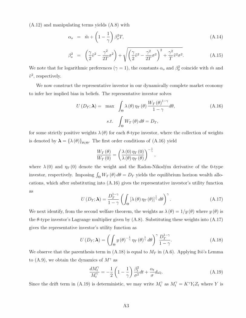
(A.12) and manipulating terms yields (A.8) with

αo = m+

(1− 1

γ

)β2oT, (A.14)

β2o =

(γ

2v2 − γ2

2Tσ2

)+

√(γ

2v2 − γ2

2Tσ2

)2

+γ2

Tv2σ2. (A.15)

We note that for logarithmic preferences (γ = 1), the constants αo and β20 coincide with m and

v2, respectively.

We now construct the representative investor in our dynamically complete market economy

to infer her implied bias in beliefs. The representative investor solves

U (DT ;λ) = max

ˆΘ

λ (θ) ηT (θ)WT (θ)1−γ

1− γdθ, (A.16)

s.t.

ˆΘ

WT (θ) dθ = DT ,

for some strictly positive weights λ (θ) for each θ-type investor, where the collection of weights

is denoted by λ = {λ (θ)}θ∈Θ. The first order conditions of (A.16) yield

WT (θ)

WT (0)=

(λ (0) ηT (0)

λ (θ) ηT (θ)

)− 1γ

,

where λ (0) and ηT (0) denote the weight and the Radon-Nikodym derivative of the 0-type

investor, respectively. Imposing´

ΘWT (θ) dθ = DT yields the equilibrium horizon wealth allo-

cations, which after substituting into (A.16) gives the representative investor’s utility function

as

U (DT ;λ) =D1−γT

1− γ

(ˆΘ

[λ (θ) ηT (θ)]1γ dθ

)γ. (A.17)

We next identify, from the second welfare theorem, the weights as λ (θ) = 1/y (θ) where y (θ) is

the θ-type investor’s Lagrange multiplier given by (A.8). Substituting these weights into (A.17)

gives the representative investor’s utility function as

U (DT ;λ) =

(ˆΘ

y (θ)−1γ ηT (θ)

1γ dθ

)γD1−γT

1− γ. (A.18)

We observe that the parenthesis term in (A.18) is equal to MT in (A.6). Applying Ito’s Lemma

to (A.9), we obtain the dynamics of Mγ as

dMγt

Mγt

= −1

2

(1− 1

γ

)β2t

σ2dt+

αtσdωt. (A.19)

Since the drift term in (A.19) is deterministic, we may write Mγt as Mγ

t = KγYtZt where Y is

A3

a deterministic process and Z is a martingale process with dynamics

dYtYt

= −1

2

(1− 1

γ

)β2t

σ2dt, (A.20)

dZtZt

=αtσdωt =

ˆΘ

θ

σ

(y (θ)−

1γ ηt (θ)

1γ´

Θy (θ)−

1γ ηt (θ)

1γ dθ

)dθdωt, (A.21)

and initial values Y0 = Z0 = 1. The solution to (A.20) is given by

Yt =

(βtβo

)γ−1

=

(σ2

σ2 + 1γβ2o t

) 12

(γ−1)

. (A.22)

Since equilibrium is unique up to a constant, we set the constant K = Y− 1γ

T in (A.8) without

loss of generality and substitute (A.20)–(A.22) to obtain the representative investor’s utility

function as

U (DT ;λ) = ZTD1−γT

1− γ,

where Z is given by the martingale process (A.21). Hence, we identify ZT as being the Radon-

Nikodym derivative of the representative investor’s subjective belief PR with respect to the true

belief P, that is dPR/dP = ZT . Moreover, (A.21) implies that αt is the time-t (stochastic) bias

of the representative investor, and so is the time-t average bias in beliefs, as denoted by mt,

mt = αt = σσαo + 1

γβ2oωt

σ2 + 1γβ2o t

=

ˆΘ

θ

(y (θ)−

1γ ηt (θ)

1γ´

Θy (θ)−

1γ ηt (θ)

1γ dθ

)dθ. (A.23)

Substituting σωt by lnDt −(µ− 1

2σ2)t yields the expression stated in (12).

From the last equality in (A.23) we identify the unique weights ht (θ) such that the weighted-

average of investors’ biases equals to the average bias in beliefs as

ht (θ) =y (θ)−

1γ ηt (θ)

1γ´

Θy (θ)−

1γ ηt (θ)

1γ dθ

. (A.24)

Substituting (A.7)–(A.8) into (A.24), and rearranging yields

ht (θ) =1√

2πβ2t

e− 1

2(θ−αt)

2

β2t , (A.25)

where αt and βt are as in (A.10) and (A.11), respectively.

Finally, to determine the belief dispersion, we use the definition in (11) with the average

bias in beliefs (A.23) and weights (A.25) substituted in to obtain

v2t =

ˆΘ

(θ −mt)2 ht (θ) dθ =

ˆΘ

(θ −mt)2 1√

2πβ2t

e− 1

2(θ−mt)

2

β2t dθ.

A4

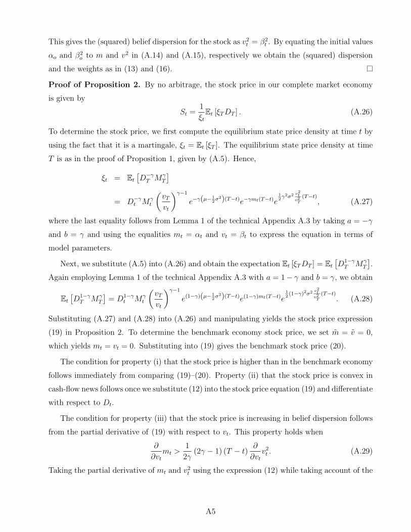
This gives the (squared) belief dispersion for the stock as v2t = β2

t . By equating the initial values

αo and β2o to m and v2 in (A.14) and (A.15), respectively we obtain the (squared) dispersion

and the weights as in (13) and (16).

Proof of Proposition 2. By no arbitrage, the stock price in our complete market economy

is given by

St =1

ξtEt [ξTDT ] . (A.26)

To determine the stock price, we first compute the equilibrium state price density at time t by

using the fact that it is a martingale, ξt = Et [ξT ]. The equilibrium state price density at time

T is as in the proof of Proposition 1, given by (A.5). Hence,

ξt = Et[D−γT Mγ

T

]= D−γt Mγ

t

(vTvt

)γ−1

e−γ(µ−12σ2)(T−t)e−γmt(T−t)e

12γ2σ2 v

2tv2T

(T−t), (A.27)

where the last equality follows from Lemma 1 of the technical Appendix A.3 by taking a = −γand b = γ and using the equalities mt = αt and vt = βt to express the equation in terms of

model parameters.

Next, we substitute (A.5) into (A.26) and obtain the expectation Et [ξTDT ] = Et[D1−γT Mγ

T

].

Again employing Lemma 1 of the technical Appendix A.3 with a = 1− γ and b = γ, we obtain

Et[D1−γT Mγ

T

]= D1−γ

t Mγt

(vTvt

)γ−1

e(1−γ)(µ− 12σ2)(T−t)e(1−γ)mt(T−t)e

12

(1−γ)2σ2 v2tv2T

(T−t). (A.28)

Substituting (A.27) and (A.28) into (A.26) and manipulating yields the stock price expression

(19) in Proposition 2. To determine the benchmark economy stock price, we set m = v = 0,

which yields mt = vt = 0. Substituting into (19) gives the benchmark stock price (20).

The condition for property (i) that the stock price is higher than in the benchmark economy

follows immediately from comparing (19)–(20). Property (ii) that the stock price is convex in

cash-flow news follows once we substitute (12) into the stock price equation (19) and differentiate

with respect to Dt.

The condition for property (iii) that the stock price is increasing in belief dispersion follows

from the partial derivative of (19) with respect to vt. This property holds when

∂

∂vtmt >

1

2γ(2γ − 1) (T − t) ∂

∂vtv2t . (A.29)

Taking the partial derivative of mt and v2t using the expression (12) while taking account of the

A5

dependency on v and m, yields

∂

∂vtmt =

2

vt(mt − m) , (A.30)

∂

∂vtv2t = 2vt, (A.31)

which after substituting into (A.29) and rearranging gives the desired condition.

Finally, property (iv) that the stock price is increasing in investors’ risk aversion for relatively

bad cash-flow states and low values of γ follows from the partial derivative of (19) with respect

to γ. This property holds when

∂

∂γmt > σ2 +

[1

2γ2v2t +

(1− 1

2γ

)(∂

∂γv2t

)](T − t) . (A.32)

In this regard, using (14)–(15), we first compute ∂v2/∂γ and ∂m/∂γ, and to simplify notation

denote them by C and D, respectively

C ≡ ∂

∂γv2 =

(v2

2− γ

Tσ2

)+

(γ2v2 − γ2

2Tσ2)(

v2

2− γ

Tσ2)

+ γTv2σ2√(

γ2v2 − γ2

2Tσ2)2

+ γ2

Tv2σ2

, (A.33)

D ≡ ∂

∂γm =

1

γ2v2T +

(1− 1

γ

)CT. (A.34)

Using the expressions (12) and (13), we then obtain the required partial derivatives as

∂

∂γmt =

v2t

v2

[D −

(1

γ− C

v2

)(mt −m)

], (A.35)

∂

∂γv2t =

v4t

v2

(C

v2+

v2t

σ2γ2

). (A.36)

Substituting (A.35) and (A.36) into (A.32) and rearranging yields the condition as

mt < m+

(1

γ− C

v2

)−1{D − v2

v2t

σ2 −[v2

2γ2+

(1− 1

2γ

)(C

v2+

v2t

σ2γ2

)v2t

](T − t)

}. (A.37)

For any time t, the right hand side of (A.37) is constant while its left hand side is the average

bias in beliefs, which is a normally distributed random variable, hence for sufficiently low levels

of mt and γ, (A.37) always holds.

Proof of Proposition 3. Applying Ito’s Lemma to the stock price (19) yields

dStSt

=

[γσ +

v2t

σ(T − t)− mt

σ

] [σ +

1

γ

v2t

σ(T − t)

]dt+

[σ +

1

γ

v2t

σ(T − t)

]dωt, (A.38)

where its drift term gives the equilibrium mean return as

µSt =

[γσ +

v2t

σ(T − t)− mt

σ

] [σ +

1

γ

v2t

σ(T − t)

]. (A.39)

A6

Substituting the equality

σ +1

γ

v2t

σ(T − t) = σ

v2t

v2T

, (A.40)

into (A.39) and manipulating gives (22). To determine the benchmark economy mean return,

we set m = v = 0, which yields mt = vt = 0. Substituting these into (A.39) gives the benchmark

mean return (23).

The condition for property (i) that the mean return is lower than in the benchmark economy

follows from comparing (22)–(23). The condition for property (ii) that the mean return is

decreasing in belief dispersion follows from the partial derivative of (22) with respect to vt.

This property holds when

∂

∂vtµSt = 2γσ2

(v2t

v2T

)∂

∂vt

(v2t

v2T

)−mt

∂

∂vt

(v2t

v2T

)− v2

t

v2T

∂

∂vtmt < 0. (A.41)

Substituting the partial derivatives (A.30)–(A.31) into (A.41) and using the equality (A.40)

and rearranging gives the desired condition.

Finally, property (iii) that the mean return is decreasing in investors’ risk aversion for

relatively bad cash-flow news and low levels of risk aversion follows from the partial derivative

of (22) with respect to γ. This property holds when

∂

∂γµSt = σ2

(v2t

v2T

)2

+

[2γσ2

(v2t

v2T

)−mt

](∂

∂γ

v2t

v2T

)− v2

t

v2T

(∂

∂γmt

)< 0. (A.42)

Substituting the partial derivatives (A.35)–(A.36) into (A.42) and using (A.40) yields

∂

∂γµSt = σ2

(v2t

v2T

)2

+

[2γσ2

(v2t

v2T

)−mt

]E − v2

t

v2T

v2t

v2

[D −

(1

γ− C

v2

)(mt −m)

], (A.43)

where we have defined E as

E ≡ ∂

∂γ

v2t

v2T

= − 1

γ2

v2t

σ2(T − t) +

1

γ

1

σ2

v4t

v2

(C

v2+

v2t

σ2γ2

)(T − t) .

Rearranging (A.43) yields the condition as

mt <

[v4t

v2T

(1

γv2− C

v4

)− E

]−1{v4t

v2T

[D

v2+

(1

γ− C

v2

)m

v2

]− σ2 v

4t

v4T

− 2γσ2 v2t

v2T

E

}. (A.44)

We note that, for any time t, the right hand side of (A.44) is a constant while its left hand

side is the average bias in beliefs, which is a normally distributed random variable, hence for

sufficiently low levels of mt (A.44) always holds.

Proof of Proposition 4. The volatility of the stock is given by the diffusion term of the

dynamics (A.38). The benchmark stock volatility readily is obtained by setting vt = 0 in the

diffusion term of (A.38).

A7

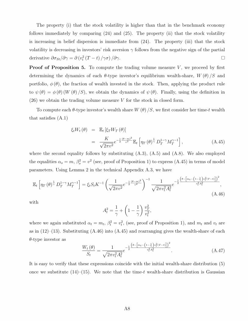
The property (i) that the stock volatility is higher than that in the benchmark economy

follows immediately by comparing (24) and (25). The property (ii) that the stock volatility

is increasing in belief dispersion is immediate from (24). The property (iii) that the stock

volatility is decreasing in investors’ risk aversion γ follows from the negative sign of the partial

derivative ∂σSt/∂γ = ∂ (v2t (T − t) /γσ) /∂γ.

Proof of Proposition 5. To compute the trading volume measure V , we proceed by first

determining the dynamics of each θ-type investor’s equilibrium wealth-share, W (θ) /S and

portfolio, φ (θ), the fraction of wealth invested in the stock. Then, applying the product rule

to ψ (θ) = φ (θ) (W (θ) /S), we obtain the dynamics of ψ (θ). Finally, using the definition in

(26) we obtain the trading volume measure V for the stock in closed form.

To compute each θ-type investor’s wealth share W (θ) /S, we first consider her time-t wealth

that satisfies (A.1)

ξtWt (θ) = Et [ξTWT (θ)]

=K√2πv2

e−12

(θ−m)2

v2 Et[ηT (θ)

1γ D1−γ

T Mγ−1T

], (A.45)

where the second equality follows by substituting (A.3), (A.5) and (A.8). We also employed

the equalities αo = m, β2o = v2 (see, proof of Proposition 1) to express (A.45) in terms of model

parameters. Using Lemma 2 in the technical Appendix A.3, we have

Et[ηT (θ)

1γ D1−γ

T Mγ−1T

]= ξtStK

−1

(1√

2πv2e−

12

(θ−m)2

v2

)−11√

2πv2tA

2t

e− 1

2

(θ−[mt−(1− 1γ )v2t (T−t)])

2

v2t A2t ,

(A.46)

with

A2t =

1

γ+

(1− 1

γ

)v2T

v2t

,

where we again substituted αt = mt, β2t = v2

t , (see, proof of Proposition 1), and mt and vt are

as in (12)–(13). Substituting (A.46) into (A.45) and rearranging gives the wealth-share of each

θ-type investor as

Wt (θ)

St=

1√2πv2

tA2t

e− 1

2

(θ−[mt−(1− 1γ )v2t (T−t)])

2

v2t A2t . (A.47)

It is easy to verify that these expressions coincide with the initial wealth-share distribution (5)

once we substitute (14)–(15). We note that the time-t wealth-share distribution is Gaussian

A8

with mean and variance

mt ≡ mt −(

1− 1

γ

)v2t (T − t) ,

v2t ≡ v2

tA2t =

1

γv2t +

(1− 1

γ

)v2T ,

as reported in Remark 1. We then apply Ito’s lemma to (A.47) to obtain the dynamics

dWt (θ)

St= . . . dt+

Wt (θ)

St

v2t

γσv2t

(θ − mt) dωt. (A.48)

To obtain each θ-type investor’s optimal portfolio φ (θ) as a fraction of wealth invested in

the stock, we match the volatility term in (A.48) with the corresponding one in

dWt (θ)

St= . . . dt+

Wt (θ)

St(φt (θ)− 1)σStdωt,

which is obtained by using (1) and (9). This yields investors’ equilibrium portfolios as

φt (θ) = 1 +v2T

γσ2v2t

(θ − mt) . (A.49)

Applying Ito’s lemma to (A.49) yields the dynamics

dφt (θ) = . . . dt− v2t v

2T

γ2σ3v2t

dωt.

We then apply the product rule to ψ (θ) = φ (θ) (W (θ) /S) to obtain the portfolio dynamics in

terms of number of shares invested in the stock ψ (θ)

dψt (θ) = . . . dt+Wt (θ)

St

v2t

γσv2t

[(θ − mt)φt (θ)− v2

T

γσ2

]dωt,

which after substituting (A.49) yields the portfolio volatility of each θ-type investor σψ (θ) as

σψt (θ) =Wt (θ)

St

v2t

γσv2t

[v2T

γσ2

((θ − mt

vt

)2

− 1

)+ vt

(θ − mt

vt

)]. (A.50)

We now compute our trading volume measure (26), obtained by summing the absolute value

of investors’ portfolio volatilities. To find this absolute value, we need to identify the types for

whom the portfolio volatility is negative at time t. From (A.50), this occurs when the square

bracket term is negative which is a quadratic in types θ. Therefore at time-t, the types for

whom the portfolio volatility σψt (θ) is negative lies between two critical types θc1 and θc2 for

which σψt (θc1) = σψt (θc2) = 0. Equating (A.50) to zero and solving the quadratic equation

A9

yields the critical types as

θc1 = mt + vt

(−1

2Xt −

1

2

√X2t + 4

), (A.51)

θc2 = mt + vt

(−1

2Xt +

1

2

√X2t + 4

), (A.52)

where Xt = γσ2vt/v2T . From definition (26), the trading volume measure is

Vt ≡1

2

ˆΘ

|σψt (θ) |dθ =1

2

[ˆ θc1

−∞σψt (θ) dθ −

ˆ θc2

θc1

σψt (θ) dθ +

ˆ ∞θc2

σψt (θ) dθ

]

= −ˆ θc2

θc1

σψt (θ) dθ, (A.53)

where the last equality follows from the fact´

Θσψt (θ) dθ = 0 which implies

ˆ θc1

−∞σψt (θ) dθ +

ˆ ∞θc2

σψt (θ) dθ = −ˆ θc2

θc1

σψt (θ) dθ.

Substituting (A.47) and (A.50) into (A.53) yields

Vt = − v2t

γσv2t

ˆ θc2

θc1

[v2T

γσ2

((θ − mt

vt

)2

− 1

)+ vt

(θ − mt

vt

)]1√2πv2

t

e− 1

2(θ−mt)

2

v2t dθ.

Changing the variable of integration to z = θ−mtvt

and using the facts thatˆ (

z2 − 1) 1√

2πe−

12z2dz = −zφ (z) + C,

ˆz

1√2πe−

12z2dz = −φ (z) + C,

where φ (.) is the standard normal density function and C is a constant, we obtain the trading

volume measure as

Vt =v2t

γσv2t

[v2T

γσ2

(θc2 − mt

vt

)+ vt

]φ

(θc2 − mt

vt

)

− v2t

γσv2t

[v2T

γσ2

(θc1 − mt

vt

)+ vt

]φ

(θc1 − mt

vt

). (A.54)

Finally, substituting (A.51)–(A.52) into (A.54) and rearranging gives (27).

The condition for property (i) that the trading volume measure is increasing in belief dis-

persion follows from the partial derivative of (27) with respect to vt, or equivalently v2. To

compute this partial derivative we rewrite (27) compactly as

Vt =1

2σ

[Z+t φ

(1

2

X2t

σ2

v2T

v2t

Z−t

)+ Z−t φ

(1

2

X2t

σ2

v2T

v2t

Z+t

)], (A.55)

A10

where we defined the positive deterministic processes

Z+t ≡

√(σ2

X2t

v2t

v2T

)2

(X2t + 4) +

σ2

Xt

v2t

v2T

,

Z−t ≡

√(σ2

X2t

v2t

v2T

)2

(X2t + 4)− σ2

Xt

v2t

v2T

,

with 0 < Z−t < Z+t , and

∂

∂v2Z+t −

∂

∂v2Z−t = 2

∂

∂v2

(σ2

Xt

v2t

v2T

). (A.56)

The partial derivative of (A.55) with respect to v2 is given by

∂

∂v2Vt =

1

2σ

[(∂Z+

t

∂v2

)φ

(1

2

X2t

σ2

v2T

v2t

Z−t

)+ Z+

t

∂

∂v2φ

(1

2

X2t

σ2

v2T

v2t

Z−t

)]

+1

2σ

[(∂Z−t∂v2

)φ

(1

2

X2t

σ2

v2T

v2t

Z+t

)+ Z−t

∂

∂v2φ

(1

2

X2t

σ2

v2T

v2t

Z+t

)]. (A.57)

Substituting

∂

∂v2φ

(1

2

X2t

σ2

v2T

v2t

Z−t

)= −1

2

X2t

σ2

v2T

v2t

Z−t φ

(1

2

X2t

σ2

v2T

v2t

Z−t

)∂

∂v2

(1

2

X2t

σ2

v2T

v2t

Z−t

),

∂

∂v2φ

(1

2

X2t

σ2

v2T

v2t

Z+t

)= −1

2

X2t

σ2

v2T

v2t

Z+t φ

(1

2

X2t

σ2

v2T

v2t

Z+t

)∂

∂v2

(1

2

X2t

σ2

v2T

v2t

Z+t

),

with

∂

∂v2

(1

2

X2t

σ2

v2T

v2t

Z−t

)=

1

2

[(X2t

σ2

v2T

v2t

)∂Z−t∂v2

+ Z−t∂

∂v2

(X2t

σ2

v2T

v2t

)],

∂

∂v2

(1

2

X2t

σ2

v2T

v2t

Z+t

)=

1

2

[(X2t

σ2

v2T

v2t

)∂Z+

t

∂v2+ Z+

t

∂

∂v2

(X2t

σ2

v2T

v2t

)],

into (A.57), and using (A.56) and the equality

Z+t Z−t = 4

(σ2

X2t

v2t

v2T

)2

,

yields the required partial derivative

∂

∂v2Vt =

1

2σ

[2∂

∂v2

(σ2

Xt

v2t

v2T

)− Z−t

σ2

X2t

v2t

v2T

∂

∂v2

(X2t

σ2

v2T

v2t

)]φ

(1

2

X2t

σ2

v2T

v2t

Z−t

)

+1

2σ

[−2

∂

∂v2

(σ2

Xt

v2t

v2T

)− Z+

t

σ2

X2t

v2t

v2T

∂

∂v2

(X2t

σ2

v2T

v2t

)]φ

(1

2

X2t

σ2

v2T

v2t

Z+t

). (A.58)

However, (A.58) is always positive because

∂

∂v2

(X2t

σ2

v2T

v2t

)< 0 and

∂

∂v2

(σ2

Xt

v2t

v2T

)> 0,

A11

which implies that the first square bracket term in (A.58) is positive, and if the second square

bracket terms is also positive then it is easy to see that (A.58) is positive. However, if the

second square bracket term is negative then we use the inequality

2∂

∂v2

(σ2

Xt

v2t

v2T

)− Z−t

σ2

X2t

v2t

v2T

∂

∂v2

(X2t

σ2

v2T

v2t

)>

∣∣∣∣−2∂

∂v2

(σ2

Xt

v2t

v2T

)− Z+

t

σ2

X2t

v2t

v2T

∂

∂v2

(X2t

σ2

v2T

v2t

)∣∣∣∣ ,and the fact that

0 < φ

(1

2

X2t

σ2

v2T

v2t

Z+t

)< φ

(1

2

X2t

σ2

v2T

v2t

Z−t

), (A.59)

to show that the first line in (A.58) dominates the second line, and therefore (A.58) is positive.

Property (ii) that the trading volume measure is positively related to the stock volatility

follows from the fact that an increase in belief dispersion leads to both a higher trading volume

measure and a stock volatility.

Finally, property (iii) that the trading volume measure is decreasing in investors’ risk aver-

sion follows from the partial derivative of (27) with respect to γ. Following the similar steps as

above, we obtain

∂

∂γVt =

1

2σ

[2∂

∂γ

(σ2

Xt

v2t

v2T

)− Z−t

σ2

X2t

v2t

v2T

∂

∂γ

(X2t

σ2

v2T

v2t

)]φ

(1

2

X2t

σ2

v2T

v2t

Z−t

)

+1

2σ

[−2

∂

∂γ

(σ2

Xt

v2t

v2T

)− Z+

t

σ2

X2t

v2t

v2T

∂

∂γ

(X2t

σ2

v2T

v2t

)]φ

(1

2

X2t

σ2

v2T

v2t

Z+t

). (A.60)

However, (A.60) is always negative because

∂

∂γ

(X2t

σ2

v2T

v2t

)> 0 and

∂

∂γ

(σ2

Xt

v2t

v2T

)< 0,

which implies the first square bracket term in (A.60) is negative, and if the second square

bracket term is also negative then it is easy to see that (A.60) is negative. However, if the

second square bracket term is positive then we use the inequality

−2∂

∂γ

(σ2

Xt

v2t

v2T

)− Z+

t

σ2

X2t

v2t

v2T

∂

∂γ

(X2t

σ2

v2T

v2t

)<

∣∣∣∣2 ∂

∂γ

(σ2

Xt

v2t

v2T

)− Z−t

σ2

X2t

v2t

v2T

∂

∂γ

(X2t

σ2

v2T

v2t

)∣∣∣∣ ,and (A.59) to show that the first line in (A.60) dominates the second line, and therefore (A.60)

is negative.

A.2 Equilibrium in Finitely-Many-Investor Economy

In this Appendix, we consider a variant of our economy in Section 2 in which there are finitely

many investors instead of a continuum of them. The other features of our economy remain

the same. In particular, the securities market is as in Section 2.1 and the investors’ beliefs are

A12

as in Section 2.2, that is, under the θn-type investor’s beliefs, the cash-flow news process has

dynamics dDt = (µ+ θn)Dtdt + σDtdωnt, where ωn is her perceived Brownian motion with

respect to her own probability measure Pθn , and is given by ωnt = ωt − θnt/σ. We again index

each θn-type investor by her bias θn, with the type space now becoming Θ = {θ1, . . . , θN} rather

than Θ = R as in our main model. We assume that each θn-type investor is initially endowed

with fn units of stock shares so that∑N

n=1 fn = 1. This gives the initial wealth of each θn-type

investor as Wn0 = S0fn. For tractability, we here only consider the case when investors have

logarithmic preferences.

As in the Proof of Proposition 1, we begin by first solving each θn-type investor’s optimiza-

tion problem. Dynamic market completeness implies a unique state price density process ξ

under P. The static budget constraint of each θn-type investor under P is given by

Et [ξTWnT ] = ξtWnt. (A.61)

We write each θn-type investor’s expected utility under the objective measure P as

E [ηnT lnWnT ] , (A.62)

where ηnT is the Radon-Nikodym derivative of the subjective measure Pθn with respect to the

true measure P given by

ηnT =dPθndP

= eθnσωT− 1

2

θ2nσ2T .

Maximizing each θn-type investor’s expected objective function (A.62) subject to (A.61) eval-

uated at time t = 0 leads to the optimal horizon wealth of each θn-type as

WnT = S0fnηnTξT

. (A.63)

Applying the market clearing condition yields the time-T equilibrium state price density as

ξT = S0D−1T

N∑n=1

fnηnT . (A.64)

The time-t equilibrium state price density is then given by ξt = Et [ξT ] which yields

ξt = S0e(σ2−µ)(T−t)D−1

t

N∑n=1

e−θn(T−t)fnηnt, (A.65)

where ηnt = Et [ηnT ] = eθnσωt− 1

2

θ2nσ2t. By no arbitrage, the stock price in this economy is given by

ξtSt = Et [ξTDT ]. Substituting (A.64)–(A.65) and computing the expectation yields the stock

price. To derive the equilibrium stock mean return and volatility, we apply Ito’s Lemma to the

stock price. These quantities presented below.

A13

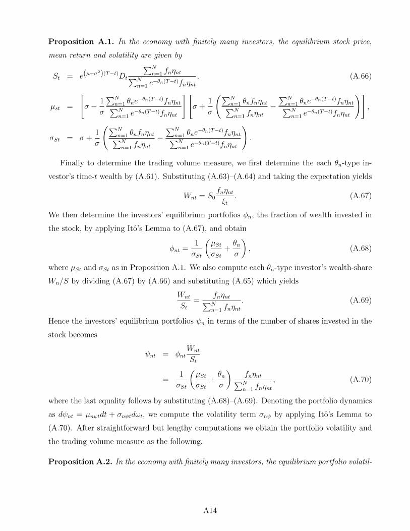
Proposition A.1. In the economy with finitely many investors, the equilibrium stock price,

mean return and volatility are given by

St = e(µ−σ2)(T−t)Dt

∑Nn=1 fnηnt∑N

n=1 e−θn(T−t)fnηnt

, (A.66)

µst =

[σ − 1

σ

∑Nn=1 θne

−θn(T−t)fnηnt∑Nn=1 e

−θn(T−t)fnηnt

][σ +

1

σ

(∑Nn=1 θnfnηnt∑Nn=1 fnηnt

−∑N

n=1 θne−θn(T−t)fnηnt∑N

n=1 e−θn(T−t)fnηnt

)],

σSt = σ +1

σ

(∑Nn=1 θnfnηnt∑Nn=1 fnηnt

−∑N

n=1 θne−θn(T−t)fnηnt∑N

n=1 e−θn(T−t)fnηnt

).

Finally to determine the trading volume measure, we first determine the each θn-type in-

vestor’s time-t wealth by (A.61). Substituting (A.63)–(A.64) and taking the expectation yields

Wnt = S0fnηntξt

. (A.67)

We then determine the investors’ equilibrium portfolios φn, the fraction of wealth invested in

the stock, by applying Ito’s Lemma to (A.67), and obtain

φnt =1

σSt

(µStσSt

+θnσ

), (A.68)

where µSt and σSt as in Proposition A.1. We also compute each θn-type investor’s wealth-share

Wn/S by dividing (A.67) by (A.66) and substituting (A.65) which yields

Wnt

St=

fnηnt∑Nn=1 fnηnt

. (A.69)

Hence the investors’ equilibrium portfolios ψn in terms of the number of shares invested in the

stock becomes

ψnt = φntWnt

St

=1

σSt

(µStσSt

+θnσ

)fnηnt∑Nn=1 fnηnt

, (A.70)

where the last equality follows by substituting (A.68)–(A.69). Denoting the portfolio dynamics

as dψnt = µnψtdt + σnψtdωt, we compute the volatility term σnψ by applying Ito’s Lemma to

(A.70). After straightforward but lengthy computations we obtain the portfolio volatility and

the trading volume measure as the following.

Proposition A.2. In the economy with finitely many investors, the equilibrium portfolio volatil-

A14

ity of each investor is given by

σnψt =φntσ

(θn −

∑Nn=1 θnfnηnt∑Nn=1 fnηnt

)Wnt

St

− 1

σ3σ2St

(θn −

∑Nn=1 θnfnηnt∑Nn=1 fnηnt

)Wnt

St

[∑Nn=1 θ

2nfnηnt∑N

n=1 fnηnt−∑N

n=1 θ2ne−θn(T−t)fnηnt∑N

n=1 e−θn(T−t)fnηnt

]

− 1

σ3σ2St

(θn −

∑Nn=1 θnfnηnt∑Nn=1 fnηnt

)Wnt

St

[2

(∑Nn=1 θnfnηnt∑Nn=1 fnηnt

)(σ2 − σσSt

)+(σ2 − σσSt

)2

]

− 1

σ2σSt

Wnt

St

∑Nn=1 θ

2nfnηnt∑N

n=1 fnηnt−

(∑Nn=1 θnfnηnt∑Nn=1 fnηnt

)2 , (A.71)

and the trading volume measure is given by

Vt =1

2

N∑n=1

|σnψt|.

where σnψt is as in (A.71).

A.3 Technical Lemmas

Lemma 1. Let the processes M , α and β be defined as in (A.9), (A.10) and (A.11), respectively.

Then for all numbers a and b we have

Et[DaTM

bT

]= Da

tMbt

(βTβt

)bea(µ−

12σ2)(T−t)e

− b2

α2tβ2t

(1−β

2Tβ2t

[1− b

γ

(1−β

2Tβ2t

)]−1)

×[1− b

γ

(1− β2

T

β2t

)]− 12

e12

[1− b

γ

(1−β

2Tβ2t

)]−1(2abαtγ

β2Tβ2t

+a2σ2

)(T−t)

, (A.72)

provided 1− bγ

(1− β2

T

β2t

)> 0.

Proof of Lemma 1. By (A.9), we have

MT = Mt

(βTβt

)e− 1

2

α2tβ2t

+ 12

α2Tβ2T , (A.73)

and (A.10)–(A.11) give

α2T

β2T

= β2T

(m2

v4+ 2

m

v2

ωTγσ

+ω2T

γ2σ2

)

=α2t

β2t

β2T

β2t

+ 2αtγσ

β2T

β2t

(ωT − ωt) +β2T

γ2σ2(ωT − ωt)2 . (A.74)

A15

Substituting (A.74) into (A.73) and using the lognormality of DT , we obtain

Et[DaTM

bT

]= Da

t ea(µ− 1

2σ2)(T−t)M b

t

(βTβt

)be− b

2

α2tβ2t

(1−β

2Tβ2t

)Et

[e

(bαtγσ

β2Tβ2t

+aσ

)(ωT−ωt)+ 1

2

bβ2Tγ2σ2

(ωT−ωt)2].

(A.75)

Let Z ∼ N (0, 1). Then the independence property of conditional expectations yields

Et

[e

(bαtγσ

β2Tβ2t

+aσ

)(ωT−ωt)+ 1

2

bβ2Tγ2σ2

(ωT−ωt)2]

= E

[e

(bαtγσ

β2Tβ2t

+aσ

)√T−tZ+ 1

2

bβ2Tγ2σ2

(T−t)Z2

]

=

ˆ ∞−∞

e

(bαtγσ

β2Tβ2t

+aσ

)√T−tz+ 1

2

bβ2Tγ2σ2

(T−t)z2 1√2πe−

12z2dz

=

[1− b

γ

(1− β2

T

β2t

)]− 12

e12

[1− b

γ

(1−β

2Tβ2t

)]−1(bαtγσ

β2Tβ2t

+aσ

)2

(T−t),

which after substituting into (A.75) and rearranging gives (A.72).

Lemma 2. Let the processes η (θ) and M be as in (A.7) and (A.9), respectively. Then

Et[ηT (θ)

1γ D1−γ

T Mγ−1T

]= ξtStK

−1

(1√

2πβ2o

e− 1

2(θ−αo)2

β2o

)−11√

2πβ2tA

2t

e− 1

2

(θ−[αt−(1− 1γ )β2t (T−t)])

2

β2t A2t ,

(A.76)

where the positive deterministic process A2 is given by

A2t =

1

γ+

(1− 1

γ

)β2T

β2t

.

Proof of Lemma 2. We first express ηT (θ)1γ in terms of DT . Using (A.7) and the lognormality

of DT , we have

ηT (θ)1γ = e

− θγσ2

(µ− 12σ2)T− 1

2γθ2

σ2TD

θγσ2

T .

Therefore, the required expectation becomes

Et[ηT (θ)

1γ D1−γ

T Mγ−1T

]= e

− θγσ2

(µ− 12σ2)T− 1

2γθ2

σ2TEt

[D

1−γ+ θγσ2

T Mγ−1T

]. (A.77)

Letting a = 1− γ + θγσ2 and b = γ − 1 in Lemma 1 of the technical Appendix A.3 yields

Et[D

1−γ+ θγσ2

T Mγ−1T

]= D

1−γ+ θγσ2

t Mγ−1t

1

At

(βTβt

)(γ−1)

e

(1−γ+ θ

γσ2

)(µ− 1

2σ2)(T−t)

e− γ−1

2

α2tβ2t

(1−β

2Tβ2t

1

A2t

)

×eαtA2t(1− 1

γ )(

1−γ+ θγσ2

)β2Tβ2t

(T−t)e

12

1

A2t

(1−γ+ θ

γσ2

)2σ2(T−t)

, (A.78)

where, for notational simplicity, we have defined the deterministic positive process

A2t ≡

1

γ+

(1− 1

γ

)β2T

β2t

.

A16

Substituting the equality

Dθγσ2

t = eθγσ2

(µ− 12σ2)t+θ

(αtβ2t−αoβ2o

),

and (A.78) into (A.77) and rearranging leads to

Et[ηT (θ)

1γ D1−γ

T Mγ−1T

]= D1−γ

t Mγ−1t

1

At

(βTβt

)(γ−1)

e(1−γ)(µ− 12σ2)(T−t)

×e−12θ2

γσ2Teθ

(αtβ2t−αoβ2o

)e− γ−1

2

α2tβ2t

(1−β

2Tβ2t

1

A2t

)

×eαtA2t(1− 1

γ )(

1−γ+ θγσ2

)β2Tβ2t

(T−t)e

12

1

A2t

(1−γ+ θ

γσ2

)2σ2(T−t)

. (A.79)

We then substitute

ξtSt = Et[D1−γT Mγ

T

]= D1−γ

t Mγt

(βTβt

)γ−1

e(1−γ)(µ− 12σ2)(T−t)e(1−γ)αt(T−t)e

12

(1−γ)2σ2 β2tβ2T

(T−t),

into (A.79) to obtain

Et[ηT (θ)

1γ D1−γ

T Mγ−1T

]= M−1

t

ξtStAt

e(γ−1)αt(T−t)e− 1

2(1−γ)2σ2 β

2tβ2T

(T−t)e− 1

2θ2

γσ2Teθ

(αtβ2t−αoβ2o

)

×e− γ−1

2

α2tβ2t

(1−β

2Tβ2t

1

A2t

)eαtA2t(1− 1

γ )(

1−γ+ θγσ2

)β2Tβ2t

(T−t)e

12

1

A2t

(1−γ+ θ

γσ2

)2σ2(T−t)

.(A.80)

Moreover, substituting the equalities

1− β2T

β2t

1

A2t

=1

A2t

β2T

γ2σ2(T − t) ,

(1− 1

γ

)β2T

γσ2(T − t) = 1− A2

t ,

and (A.9) into (A.80) yields

Et[ηT (θ)

1γ D1−γ

T Mγ−1T

]= ξtStK

−1

(1√

2πβ2o

e− 1

2(θ−αo)2

β2o

)−11√

2πβ2tA

2t

×e−12

(θ−αo)2

β2o e12

α2oβ2o− 1

2

α2tβ2t e(γ−1)αt(T−t)e

− 12

(1−γ)2σ2 β2tβ2T

(T−t)e− 1

2θ2

γσ2Teθ

(αtβ2t−αoβ2o

)

×e− γ−1

2

α2tβ2t

1

A2t

β2Tγ2σ2

(T−t)eαtA2t

(1−γ+ θ

γσ2

)γσ2

β2t(1−A2

t)e

12

1

A2t

(1−γ+ θ

γσ2

)2σ2(T−t)

.

We note that the last three rows in the above equation is equal to

e− 1

2

(θ−[αt−(1− 1γ )β2t (T−t)])

2

β2t A2t ,

and so we obtain (A.76).

A17

Internet Appendix for “Belief Dispersion in the Stock

Market”

B Appendix: Proofs of Bayesian Economy

Proof of Proposition 6. We proceed by first finding the optimal estimate of the mean growth

rate of the expected payoff µ for each θ-type investor and elicit their respective beliefs. We

then proceed as in the proof of Proposition 1 in Appendix A.

Following the standard filtering theory (see, Liptser and Shiryaev (2001)), for each θ-

type investor, the time-t posterior distribution of µ, conditional on the information set Ft =

{Du : 0 ≤ u ≤ t}, is normally distributed, N (µ+ θt, s2t ), where the time-t bias of θ-type investor

θt and the type-independent mean squared error s2t are given by

dθt =s2t

σdωt (θ) , (B.1)

s2t =

s2σ2

σ2 + s2t, (B.2)

and her perceived Brownian motion process ω (θ) is given by

dωt (θ) =1

σ

(dDt

Dt

− (µ+ θt)dt

)= dωt −

θtσdt,

which implies the likelihood process η (θ) of

dηt (θ) = ηt (θ)θtσdωt,

ηt (θ) = e´ t0θuσdωu− 1

2

´ t0

(θuσ

)2du. (B.3)

Solution to (B.1) (θ-type investor’s bias at time t) is given by

θt = σσθ + s2ωtσ2 + s2t

=s2t

s2θ +

s2t

σωt.

Substituting this into (B.3) and solving yields the likelihood process as

ηt (θ) =stse− 1

2θ2

s2+ 1

2

θ2ts2t . (B.4)

Each θ-investor’s maximization problem

Eθ[WT

1−γ

1− γ

],

B1

subject to the budget constraint

dWt (θ) = φt (θ)Wt (θ) (µSt (θ) dt+ σStdωt (θ)) ,

µSt (θ) = µSt + σStθtσ,

where the expectation is taken such that ω (θ) is a standard Brownian motion, can be solved

using standard martingale techniques.

Following similar steps as in the proof of Proposition 1 in Appendix A, we obtain the optimal

horizon wealth of each θ-type as

WT (θ) =

(ηT (θ)

y (θ) ξT

) 1γ

, (B.5)

where ηT (θ) is (B.4) evaluated at time T and the Lagrange multiplier y (θ) solves

y (θ)−1γ = E

[ηT (θ)

1γ ξ

1− 1γ

T

]−1ξ0S0√2πv2

e−12

(θ−m)2

v2 .

The time-T equilibrium state price density ξT is again given by ξT = D−γT MγT , where the

auxiliary process M is defined as Mt ≡´

Θy (θ)−

1γ ηt (θ)

1γ dθ. As we show below, y (θ)−

1γ is

(scaled) Gaussian over the type space Θ for some mean αo, variance β2o and a constant K:

y (θ)−1γ = K

1√2πβ2

o

e− 1

2(θ−αo)2

β2o . (B.6)

Substituting (B.4) and (B.6) into the definition of M yields

Mt = K

ˆR

1√2πβ2

o

e− 1

2(θ−αo)2

β2o

(sts

) 1γe− 1

21γθ2

s2+ 1

21γ

θ2ts2t dθ = K

βtβoe− 1

2

α2oβ2o

+ 12

α2tβ2t

(sts

) 1γe

12

s2tγ

ω2tσ2 , (B.7)

where the last equality follows by completing the square and integrating, and the processes α

and β are

αt =(σ2 + s2t)αo + σ 1

γβ2oωt

(σ2 + s2t) + 1γβ2o t

, (B.8)

β2t =

β2o (σ2 + s2t)

(σ2 + s2t) + 1γβ2o t, (B.9)

with their initial values given by α0 = αo and β0 = βo, respectively.

Following similar steps as in the proof of Proposition 1 in Appendix A, we verify y (θ)−1γ is

B2

as in (B.6) with

αo = m+

(1− 1

γ

)β2oT, (B.10)

β2o =

(γ

2v2 − γ2

2T

(σ2 + s2T

))+

√(γ

2v2 − γ2

2T(σ2 + s2T )

)2

+γ2

Tv2 (σ2 + s2T ). (B.11)

The construction of the representative investor is as in the dogmatic beliefs case in the proof

of Proposition 1 in Appendix A, which in this case yields the time-t average bias in beliefs mt

as

mt = αt = σσαo +

(1γβ2o + s2

)ωt

σ2 +(

1γβ2o + s2

)t

=

ˆΘ

θt

(y (θ)−

1γ ηt (θ)

1γ´

Θy (θ)−

1γ ηt (θ)

1γ dθ

)dθ. (B.12)

Substituting σωt = lnDt −(µ− 1

2σ2)t yields the expression stated in (30).

From the last equality in (B.12) we identify the unique weights ht (θ) such that the weighted-

average of investors’ biases equals to the average bias in beliefs as

ht (θ) =y (θ)−

1γ ηt (θ)

1γ´

Θy (θ)−

1γ ηt (θ)

1γ dθ

. (B.13)

Substituting (B.4) and (B.6) into (B.13), and rearranging yields

ht (θ) =1√

2πβ2t

e− 1

2(θ−αt)

2

β2t =1√

2πβ2t (s4

t/s4)e− 1

2

(θt−αt)2

β2t (s4t /s4)s2t

s2, (B.14)

where αt and βt are as in (B.8) and (B.9), respectively.

Finally, to determine the belief dispersion, we use definition (29) with the average bias in

beliefs (B.12) and weights (B.14) substituted in to obtain

v2t =

ˆΘ

(θt −mt

)2

ht (θ) dθ =

ˆ ∞−∞

(θt − αt

)2 1√2πβ2

t (s4t/s

4)e− 1

2

(θt−αt)2

β2t (s4t /s4)s2t

s2

(s2t

s2

)−1

dθt.

This gives the (squared) belief dispersion for the stock as

v2t = β2

t

s4t

s4.

By equating the initial values αo and β2o to m and v2 in (B.10)–(B.11), respectively we obtain

the (squared) dispersion and the weights as in (31) and (35).

The condition for property (i) that the average bias in beliefs is increasing in parameter

uncertainty follows from the partial derivative of (30) with respect to st (or, equivalently with

B3

respect to s2, since ∂s2/∂st > 0). This property holds when Dt > exp((m+ µ− 1

2σ2)t), since

∂mt

∂s2=

(lnDt −

(m+ µ− 1

2σ2

)t

)σ2(

σ2 +(

1γv2 + s2

)t)2 . (B.15)

The property (ii) that the dispersion in beliefs is decreasing in parameter uncertainty follows

from the partial derivative of (31) with respect to s2, since

∂v2t

∂s2= −v2σ2

2 (σ2 + s2t) + 1γv2t

(σ2 + s2t)2

σ2(σ2 +

(1γv2 + s2

)t)2 t < 0.

Proof of Proposition 7. To determine the stock price, we first compute the equilibrium state

price density at time t by using the fact that it is a martingale, ξt = Et [ξT ]. The equilibrium

state price density at time T is as in the proof of Proposition 6 in Appendix B, given by

ξT = D−γT MγT . Hence,

ξt = Et[D−γT Mγ

T

]= D−γt Mγ

t

(vTvt

s2t

s2T

)γ−1

e−[γ(µ− 1

2σ2)+ 1

2(mtσ )2 v2Tv2t

s2ts2T

− 12σ2 v

2tv2T

s2Ts2t

(mtσ2

v2Tv2t

s2ts2T

−γ)2]

(T−t), (B.16)

where the last equality follows from Lemma 3 at the end of the Internet Appendix B by taking

a = −γ and b = γ and using the equalities mt = αt and vt = βt (s2t/s

2) to express the equation

in terms of model parameters.

Next, we compute the expectation Et [ξTDT ] = Et[D1−γT Mγ

T

]. Again, employing Lemma 3

at the end of the Internet Appendix B with a = 1− γ and b = γ, we obtain

Et[D1−γT Mγ

T

]= D1−γ

t Mγt

(vTvt

s2t

s2T

)γ−1

e(1−γ)

[(µ− 1

2σ2)+mt+

12

(1−γ)σ2 v2tv2T

s2Ts2t

](T−t)

. (B.17)

By no arbitrage, the stock price in our complete market economy is again given by (A.26).

Substituting (B.16) and (B.17) into (A.26) and manipulating yields (37).

To determine the mean return, we apply Ito’s Lemma to the stock price (37) and obtain

dStSt

=

[(γσ

v2t

v2T

s2T

s2t

− mt

σ

)σv2t

v2T

s2T

s2t

]dt+

[σ +

1

σ

(1

γv2 + s2

)v2t

v2

s2

s2t

(T − t)]dωt. (B.18)

The drift term in (B.18) gives the equilibrium mean return.

The condition for property (i) that the stock price is increasing in parameter uncertainty

follows from the partial derivative of (37) with respect to s2t (or, equivalently with respect to

s2, since ∂s2/∂st > 0). This property holds if and only if ∂St/∂s2 > 0, which is given by the

B4

condition∂

∂s2mt >

1

2(2γ − 1) (T − t) ∂

∂s2

((1

γv2 + s2

)v2t

v2

s2

s2t

). (B.19)

Substituting (B.15) and

∂

∂s2

((1

γv2 + s2

)v2t

v2

s2

s2t

)=

σ4(σ2 +

(1γv2 + s2

)t)2 ,

into (B.19) and rearranging gives the required condition.

The condition for property (ii) that the mean return is decreasing in parameter uncertainty

follows from the partial derivative of (38) with respect to s2. This property holds if and only

if ∂µSt/∂s2 < 0, which is given by the condition

2γσ2 v2t

v2T

s2T

s2t

∂

∂s2

(v2t

v2T

s2T

s2t

)<v2t

v2T

s2T

s2t

∂

∂s2mt +mt

∂

∂s2

(v2t

v2T

s2T

s2t

),

substituting (B.15) along with

∂

∂s2

(v2t

v2T

s2T

s2t

)=

σ2 (T − t)(σ2 +

(1γv2 + s2

)t)2 ,

and rearranging gives the required condition.

We now prove that properties in Propositions 2–3 also hold in this more general economy.

The condition for property that the stock price is higher than in the benchmark economy follows

immediately by comparing (20) and (37). The property that the stock price is convex in cash-

flow news follows once we substitute (30) into the stock price equation (37). The condition for

property that the stock price is increasing in belief dispersion follows from the partial derivative

of (37) with respect to vt. This property holds when

mt > m+1

2(2γ − 1)

(1

γv2 + s2

)v2t

v2

s2

s2t

(T − t)− (γ − 1) s2T.

The property that the stock price is increasing in investors’ risk aversion for relatively bad

cash-flow states and low values of γ follows from the partial derivative of (37) with respect to

γ. This property holds when

mt < mσ2

σ2 +(

1γv2 + s2

)t

+K1t −K2t

σ2

(σ2+( 1γv2+s2)t)

3v2σ4

γ2( 1γv2+s2)

(1− γ

v2∂v2

∂γ

) ,

B5

where the deterministic processes K1, K2 are defined as

K1t ≡ σ2

(σ2 +

(1γv2 + s2

)t)(

1γv2 + 1− γ

)T +m v2

γ2

(1− γ

v2∂v2

∂γ

)t(

σ2 +(

1γv2 + s2

)t)2 , (B.20)

K2t ≡ σ2 v2t

v2T

s2T

s2t

− 1

2(2γ − 1)

v2

γ2

σ8(σ2 +

(1γv2 + s2

)t)4

(1− γ

v2

∂v2

∂γ

)(T − t) ,

and

1− γ

v2

∂v2

∂γ=

1

2

γ2

T

(σ2 + s2T )

v2

1 +

(γ2v2 − γ2

2T(σ2 + s2T )

)√(

γ2v2 − γ2

2T(σ2 + s2T )

)2

+ γ2

Tv2 (σ2 + s2T )

> 0. (B.21)

Similarly, the condition for property that the mean return is lower than in the benchmark

economy follows from comparing (23) and (38). The condition for property that the mean

return is decreasing in belief dispersion follows from the partial derivative of (38) with respect

to vt. This property holds when

mt >m+ 2γσ2

(v2tv2T

s2Ts2t− 1)− (γ − 1) s2T

2− v2Tv2t

s2ts2T

.

The property that the mean return is decreasing in investors’ risk aversion for relatively bad

cash-flow news and low levels of risk aversion follows from the partial derivative of (38) with

respect to γ. This property holds when

mt <

σv2tv2T

s2Ts2t

(K1t

(σ2+( 1γv2+s2)t)

2

σ2 +K3t

)−K4t

v4t σ

v2γ2s4

s4t

(2 (T − t) +

σ2+( 1γv2+s2)t

1γv2+s2

)(1− γ

v2∂v2

∂γ

) ,where K1 is as in (B.20) and the deterministic processes K3, K4 are defined as

K3t ≡ mσ6(

σ2 +(

1γv2 + s2

)t)2

v2

γ2(

1γv2 + s2

) (1− γ

v2

∂v2

∂γ

),

K4t ≡ σ

(σ2 +

(1

γv2 + s2

)T

)2

+ 2v6t

v2T

s2T

s6t

s4σ3

v2γ

(1− γ

v2

∂v2

∂γ

)(T − t) .

Proof of Proposition 8. The volatility of the stock is given readily by the diffusion term in

the dynamics (B.18).

To compute the trading volume measure V , we proceed as in the proof of Proposition 5 in

B6

Appendix A by first determining the dynamics of each θ-type investor’s equilibrium wealth-

share W (θ) /S and portfolio φ (θ) as the fraction of wealth invested in the stock. Then, we

apply the product rule to ψ (θ) = φ (θ) (W (θ) /S) to obtain the dynamics of the number of

shares invested in the stock ψ (θ). Finally, using the definition (26) we obtain the trading

volume measure V for the stock.

We begin by first computing each θ-type investor’s wealth share W (θ) /S. The time-t wealth

of θ-type investor is given by

ξtWt (θ) = Et [ξTWT (θ)]

= K1√

2πv2e−

12

(θ−m)2

v2 Et[ηT (θ)

1γ D1−γ

T Mγ−1T

], (B.22)

where the second equality follows by substituting (B.5), (B.6) and ξT = D−γT MγT . We have

also employed the equalities αo = m, β2o = v2 (see, proof of Proposition 6 in Appendix B), to

express (B.22) in terms of the model parameters. Using similar steps as in the proof of Lemma

2 in the technical Appendix A.3, the expectation in (B.22) can be shown to

Et[ηT (θ)

1γ D1−γ

T Mγ−1T

]= ξtStK

−1

(1√

2πv2e−

12

(θ−m)2

v2

)−11√

2πv2tA

2t

e− 1

2

(θt−[mt−(1− 1γ )v2t (T−t)])

2

v2t A2t

s2t

s2,

(B.23)

where the positive deterministic process A is given by

A2t =

1

γ+

(1− 1

γ

)v2T

v2t

s4t

s4T

,

and mt and vt are as in (30)–(31). Substituting (B.23) into (B.22) and rearranging gives the

wealth-share of each θ-type investor as

Wt (θ)

St=

1√2πv2

tA2t

e− 1

2

(θt−[mt−(1− 1γ )v2t (T−t)])

2

v2t A2t

s2t

s2. (B.24)

Hence the time-t wealth-share weighted average bias and (squared) dispersion are given by

mt ≡ˆ

Θ

θtWt (θ)

Stdθ = mt −

(1− 1

γ

)v2t (T − t) ,

v2t ≡

ˆΘ

(θt − mt

)2 Wt (θ)

Stdθ = v2

tA2t =

1

γv2t +

(1− 1

γ

)v2T

s4t

s4T

,

and applying Ito’s lemma to (B.24) yields the dynamics for the wealth-share as

dWt (θ)

St= . . . dt+

Wt (θ)

St

v2t

γσv2t

(θt − mt

)dωt. (B.25)

To obtain each θ-type investor’s optimal portfolio φ (θ) as a fraction of wealth invested in

B7

the stock, we match the volatility term in (B.25) with the corresponding one in

dWt (θ)

St= . . . dt+

Wt (θ)

St(φt (θ)− 1)σStdωt,

which yields investors’ equilibrium portfolios as

φt (θ) = 1 +v2T

γσ2v2t

s2t

s2T

(θt − mt

). (B.26)

Applying Ito’s lemma to (B.26) yields the dynamics

dφt (θ) = . . . dt− v2t v

2T

γ2σ3v2t

s2t

s2T

dωt.

Finally, applying the product rule to ψ (θ) = φ (θ) (W (θ) /S) yields

dψt (θ) = . . . dt+Wt (θ)

St

v2t

γσv2t

[(θt − mt

)φt (θ)− v2

T

γσ2

s2t

s2T

]dωt,

which after substituting (B.26) gives the portfolio volatility of each θ-type investor σψ (θ) as

σψt (θ) =Wt (θ)

St

v2t

γσv2t

v2T

γσ2

s2t

s2T

( θt − mt

vt

)2

− 1

+ vt

(θt − mt

vt

) .Following similar steps as in the proof of Proposition 5 in Appendix A, we obtain the trading

volume measure as

Vt =σ

X2t

v2t

v2T

s2T

s2t

(1

2Xt +

1

2

√X2t + 4

)φ

(1

2Xt −

1

2

√X2t + 4

)

− σ

X2t

v2t

v2T

s2T

s2t

(1

2Xt −

1

2

√X2t + 4

)φ

(1

2Xt +

1

2

√X2t + 4

),

where the positive deterministic process X is defined as

X2t ≡

γ2σ4

v4T

[1

γv2t

s4T

s4t

+

(1− 1

γ

)v2T

].

The property (i) that the stock volatility is increasing in parameter uncertainty follows

from the partial derivative of (39) with respect to s2t (or, equivalently with respect to s2, since

∂s2/∂st > 0). This property holds since

∂σSt∂s2

=σ3 (T − t)(

σ2 +(

1γv2 + s2

)t)2 > 0.

Property (ii) that the effect of parameter uncertainty on stock volatility is decreasing as the

dispersion increases follows from the cross partial derivative ∂2σSt/∂v2∂s2. This property holds

since∂

∂v2

(∂σSt∂s2

)= −2

γ

σ3t (T − t)(σ2 +

(1γv2 + s2

)t)3 < 0.

B8

The condition for property (iii) that the trading volume is decreasing in parameter uncertainty

for γ ≥ 1 follows from the partial derivative of (40) with respect to s2. To compute this partial

derivative we rewrite (40) as

Vt =1

2σ

[Z+t φ

(Z−t2

X2t v

2T s

2t

σ2v2t s

2T

)+ Z−t φ

(Z+t

2

X2t v

2T s

2t

σ2v2t s

2T

)], (B.27)

where we have defined the positive deterministic processes

Z+t ≡

√(σ2v2

t s2T

X2t v

2T s

2t

)2

(X2t + 4) +

σ2v2t s

2T

Xtv2T s

2t

,

Z−t ≡

√(σ2v2

t s2T

X2t v

2T s

2t

)2

(X2t + 4)− σ2v2

t s2T

Xtv2T s

2t

,

with 0 < Z−t < Z+t , and

∂

∂s2Z+t −

∂

∂s2Z−t = 2

∂

∂s2

(σ2v2

t s2T

Xtv2T s

2t

). (B.28)

The partial derivative of (B.27) with respect to s2 is given by

∂

∂s2Vt =

1

2σ

[(∂

∂s2Z+t

)φ

(Z−t2

X2t v

2T s

2t

σ2v2t s

2T

)+ Z+

t

∂

∂s2φ

(Z−t2

X2t v

2T s

2t

σ2v2t s

2T

)]

+1

2σ

[(∂

∂s2Z−t

)φ

(Z+t

2

X2t v

2T s

2t

σ2v2t s

2T

)+ Z−t

∂

∂s2φ

(Z+t

2

X2t v

2T s

2t

σ2v2t s

2T

)]. (B.29)

Substituting

∂

∂s2φ

(Z−t2

X2t v

2T s

2t

σ2v2t s

2T

)= −Z

−t

2

X2t v

2T s

2t

σ2v2t s

2T

φ

(Z−t2

X2t v

2T s

2t

σ2v2t s

2T

)∂

∂s2

(Z−t2

X2t v

2T s

2t

σ2v2t s

2T

),

∂

∂s2φ

(Z+t

2

X2t v

2T s

2t

σ2v2t s

2T

)= −Z

+t

2

X2t v

2T s

2t

σ2v2t s

2T

φ

(Z+t

2

X2t v

2T s

2t

σ2v2t s

2T

)∂

∂s2

(Z+t

2

X2t v

2T s

2t

σ2v2t s

2T

),

with

∂

∂s2

(Z−t2

X2t v

2T s

2t

σ2v2t s

2T

)=

1

2

[(X2t v

2T s

2t

σ2v2t s

2T

)∂

∂s2Z−t + Z−t

∂

∂s2

(X2t v

2T s

2t

σ2v2t s

2T

)],

∂

∂s2

(Z+t

2

X2t v

2T s

2t

σ2v2t s

2T

)=

1

2

[(X2t v

2T s

2t

σ2v2t s

2T

)∂

∂s2Z+t + Z+

t

∂

∂s2

(X2t v

2T s

2t

σ2v2t s

2T

)],

into (B.29), and using the equalities (B.28) and

Z+t Z−t = 4

(σ2v2

t s2T

X2t v

2T s

2t

)2

,

B9

yields the required partial derivative

∂

∂s2Vt =

1

2σ

[2∂

∂s2

(σ2v2

t s2T

Xtv2T s

2t

)− Z−t

σ2v2t s

2T

Xtv2T s

2t

∂

∂s2

(X2t v

2T s

2t

σ2v2t s

2T

)]φ

(Z−t2

X2t v

2T s

2t

σ2v2t s

2T

)

+1

2σ

[−2

∂

∂s2

(σ2v2

t s2T

Xtv2T s

2t

)− Z+

t

σ2v2t s

2T

Xtv2T s

2t

∂

∂s2

(X2t v

2T s

2t

σ2v2t s

2T

)]φ

(Z+t

2

X2t v

2T s

2t

σ2v2t s

2T

). (B.30)

However, (B.30) is always negative for γ ≥ 1 because

∂

∂s2

(X2t v

2T s

2t

σ2v2t s

2T

)> 0 and

∂

∂s2

(σ2v2

t s2T

Xtv2T s

2t

)< 0, for γ ≥ 1,

which implies that for γ ≥ 1, the first square bracket term in (B.30) is negative, and if the second

square bracket term is also negative then it is easy to see that (B.30) is negative. However, if

the second square bracket term is positive then we use the inequality

−2∂

∂s2

(σ2v2

t s2T

Xtv2T s

2t

)−Z+

t

σ2v2t s

2T

Xtv2T s

2t

∂

∂s2

(X2t v

2T s

2t

σ2v2t s

2T

)<

∣∣∣∣2 ∂

∂s2

(σ2v2

t s2T

Xtv2T s

2t

)− Z−t

σ2v2t s

2T

Xtv2T s

2t

∂

∂s2

(X2t v

2T s

2t

σ2v2t s

2T

)∣∣∣∣ ,and the fact that

0 < φ

(Z+t

2

X2t v

2T s

2t

σ2v2t s

2T

)< φ

(Z−t2

X2t v

2T s

2t

σ2v2t s

2T

), (B.31)

to show that the first line in (B.30) dominates the second line, and therefore (B.30) is negative

when γ ≥ 1.

We now prove that properties in Propositions 4–5 also hold in this more general economy.

The property that the stock volatility is higher than that in the benchmark economy follows

immediately by comparing (25) and (39). The property that the stock volatility is increasing in

belief dispersion is also immediate from (39). The property that the stock volatility is decreasing

in investors’ risk aversion follows from the negative sign of the partial derivative of (39) with

respect to γ∂σSt∂γ

= − σ7(σ2 +

(1γv2 + s2

)t)4

v2

γ2

(1− γ

v2

∂v2

∂γ

)(T − t) < 0,

where 1− (γ/v2)(∂v2/∂γ) is positive and as in (B.21) .

Similarly, the condition for property that the trading volume measure is increasing in belief

dispersion follows from the partial derivative of (40) with respect to vt, or equivalently v2.

Following similar steps as in the case with respect to s2 above, we obtain

∂

∂v2Vt =

1

2σ

[2∂

∂v2

(σ2v2

t s2T

Xtv2T s

2t

)− Z−t

σ2v2t s

2T

X2t v

2T s

2t

∂

∂v2

(X2t v

2T s

2t

σ2v2t s

2T

)]φ

(Z−t2

X2t v

2T s

2t

σ2v2t s

2T

)

+1

2σ

[−2

∂

∂v2

(σ2v2

t s2T

Xtv2T s

2t

)− Z+

t

σ2v2t s

2T

X2t v

2T s

2t

∂

∂v2

(X2t v

2T s

2t

σ2v2t s

2T

)]φ

(Z+t

2

X2t v

2T s

2t

σ2v2t s

2T

). (B.32)

B10

However, (B.32) is always positive because

∂

∂v2

(X2t v

2T s

2t

σ2v2t s

2T

)< 0 and

∂

∂v2

(σ2v2

t s2T

Xtv2T s

2t

)> 0,

which implies that the first square bracket term in (B.32) is positive, and if the second square

bracket term is also positive then it is easy to see that (B.32) is positive. However, if the second

square bracket term is negative then we use the inequality

2∂

∂v2

(σ2v2

t s2T

Xtv2T s

2t

)−Z−t

σ2v2t s

2T

X2t v

2T s

2t

∂

∂v2

(X2t v

2T s

2t

σ2v2t s

2T

)>

∣∣∣∣−2∂

∂v2

(σ2v2

t s2T

Xtv2T s

2t

)− Z+

t

σ2v2t s

2T

X2t v

2T s

2t

∂

∂v2

(X2t v

2T s

2t

σ2v2t s

2T

)∣∣∣∣ ,and (B.31) to show that the first line in (B.32) dominates the second line, and therefore (B.32)

is positive. The property that the trading volume measure is positively related to the stock

volatility follows from the fact that an increase in belief dispersion leads to both a higher trading

volume measure and a stock volatility as before. Finally, the property that the trading volume

measure is decreasing in investors’ risk aversion follows from the partial derivative of (40) with

respect to γ. Following similar steps as in the case with respect to s2 again, we obtain

∂

∂γVt =

1

2σ

[2∂

∂γ

(σ2v2

t s2T

Xtv2T s

2t

)− Z−t

σ2v2t s

2T

Xtv2T s

2t

∂

∂γ

(X2t v

2T s

2t

σ2v2t s

2T

)]φ

(Z−t2

X2t v

2T s

2t

σ2v2t s

2T

)

+1

2σ

[−2

∂

∂γ

(σ2v2

t s2T

Xtv2T s

2t

)− Z+

t

σ2v2t s

2T

Xtv2T s

2t

∂

∂γ

(X2t v

2T s

2t

σ2v2t s

2T

)]φ

(Z+t

2

X2t v

2T s

2t

σ2v2t s

2T

). (B.33)

However, (B.33) is always negative because

∂

∂γ

(X2t v

2T s

2t

σ2v2t s

2T

)> 0 and

∂

∂γ

(σ2v2

t s2T

Xtv2T s

2t

)< 0,

which implies that the first square bracket term in (B.33) is negative, and if the second square

bracket term is also negative then it is easy to see that (B.33) is negative. However, if the

second square bracket term is positive then we use the inequality

−2∂

∂γ

(σ2v2

t s2T

Xtv2T s

2t

)−Z+

t

σ2v2t s

2T

Xtv2T s

2t

∂

∂γ

(X2t v

2T s

2t

σ2v2t s

2T

)<

∣∣∣∣2 ∂

∂γ

(σ2v2

t s2T

Xtv2T s

2t

)− Z−t

σ2v2t s

2T

Xtv2T s

2t

∂

∂γ

(X2t v

2T s

2t

σ2v2t s

2T

)∣∣∣∣ ,and (B.31) to show that the first line in (B.33) dominates the second line, and therefore (B.33)

is negative.

Lemma 3. Let the processes M , α and β be as in (B.7), (B.8) and (B.9), respectively. Then

for all numbers a and b we have

Et[DaTM

bT

]= Da

tMbt

(βTβt

)b(sTst

) bγ

ea(µ−12σ2)(T−t)e

− 12bγ

(αtσ

)2 β2Tβ2t

s2Ts2t

(T−t)

×[1− b

γ

(1− β2

T

β2t

s2T

s2t

)]− 12

e12

[1− b

γ

(1−β

2Tβ2t

s2Ts2t

)]−1(bγαtσ2

β2Tβ2t

s2Ts2t

+a

)2

σ2(T−t),(B.34)

B11

provided 1− bγ

(1− β2

T

β2t

s2Ts2t

)> 0.

Proof of Lemma 3. By (B.7), we have

MT = Mt

(βTβt

)(sTst

) 1γ

e− 1

2

α2tβ2t

+ 12

α2Tβ2T e

+ 12γs2

[s2

s2T

(αTβ2T

−αoβ2o

)2

− s2

s2t

(αtβ2t−αoβ2o

)2],

which after rearranging this and using (B.8)–(B.9) lead to

MT = Mt

(βTβt

)(sTst

) 1γ

eG0t(T−t)+G1t(ωT−ωt)

σ+ 1

2G2t

(ωT−ωt)2

σ2 ,

where the time-t measurable processes G0, G1, and G2 are defined as

G0t ≡ −1

2

1

γ

(αtσ

)2β2T

β2t

s2T

s2t

, G1t ≡αtγ

β2T

β2t

s2T

s2t

, G2t ≡β2T

γ2

s4T

s4+s2T

γ,

and αt is given by (B.12). Therefore, using the lognormality of DT we obtain the expectation

Et[DaTM

bT

]= Da

t ea(µ− 1

2σ2)(T−t)M b

t

(βTβt

)b(sTst

) bγ

ebG0t(T−t)Et[e(b

G1tσ

+aσ)(ωT−ωt)+ 12bG2tσ2

(ωT−ωt)2].

(B.35)

To compute the expectation in (B.35), we let Z ∼ N (0, 1) and use the independence property

of conditional expectations to obtain

Et[e(b

G1tσ

+aσ)(ωT−ωt)+ 12bG2tσ2

(ωT−ωt)2]

= E[e(b

G1tσ

+aσ)√T−tZ+ 1

2bG2tσ2

(T−t)Z2]

=

[1− bG2t

σ2(T − t)

]− 12

e12 [1−bG2t

σ2(T−t)]

−1(bG1t

σ+aσ)

2(T−t).

Substituting the last line into (B.35) and rearranging gives (B.34).

B12