bernard, eaton, jensen kortum (bejk) -...

An Alternative Theory of the Plant Size Distribution,

with Geography and Intra- and International Trade

Holmes and Stevens (2012)

Standard Theory of the Within—Industry Size Distribution

• New plants enter an industry and obtain a productivity draw.Plants that get good draws choose to be big. Lucas (1978)

• This idea has widespread use in international to explain tradefacts.

— Melitz

— Bernard, Eaton, Jensen Kortum (BEJK)

This Paper

• Observation: Even when we go to narrowly-defined industries,big plants often do not look like homothetic expansions of

smaller plants

• Plants of different size tend to do different functions. (Pioreand Sable (1984))

— Small plants: Specialty goods, craft production, (custom,

retail-like)

— Large plants: Standardized goods for inventory, mass pro-

duction

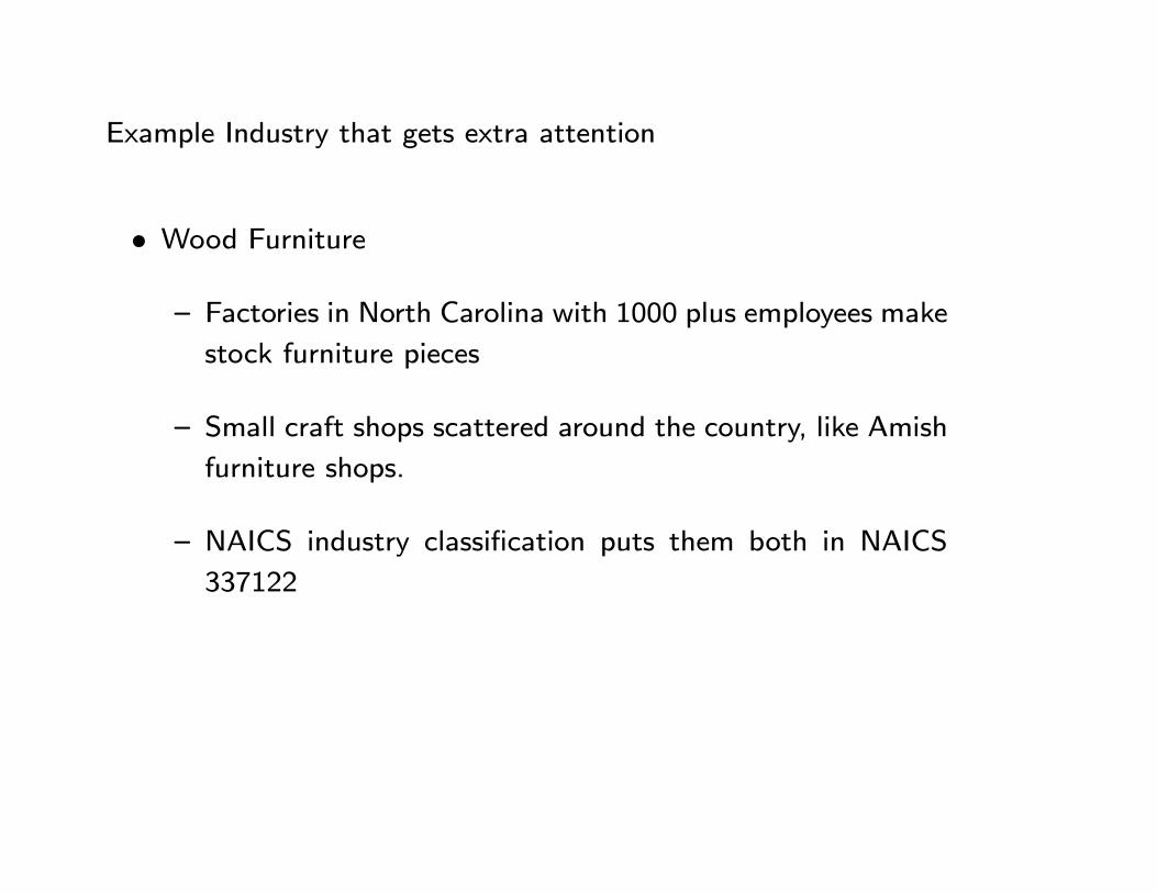
Example Industry that gets extra attention

• Wood Furniture

— Factories in North Carolina with 1000 plus employees make

stock furniture pieces

— Small craft shops scattered around the country, like Amish

furniture shops.

— NAICS industry classification puts them both in NAICS

337122

What We Do

• Theory of Geography and Trade applied to locations in theU.S.

— Standardized goods (off-the-shelf BEJK)

— Specialty goods

• Estimate the model

— Use Census micro data on the Commodity Flow Data

• Result 1: Estimate the share of establishment counts in thespecialty good segments

— In most industries, more then half the plants are specialtygood plants

— In most industries, the share is growing.

• Result 2: Concerns the plant size/industry concentration re-lationship

— Pure BEJK special case bombs quantitatively (can get thisqualitatively)

— Model with specialty goods segment added fits this

• Result 3: What happens when imports from China begin flow-ing into an industry?

As an illustration, the impact of China on the wood furniture in-

dustry...

• U.S. industry has collapsed over period 1997-2007.

• Standard model predicts NC share of what is left should rise.

• Big screwup!

• Places like High Point, N.C. vs. places like New York.

Four Basic Facts about the Within-Industry (6-digit NAICS) Size

Distribution

1. Enormous variation in plant size.

• Variance in ln(emp)=1.55 in overall manufacturing.

• 82% remains when difference out industry means.

2. Skewed right, large fraction of small plants.

• Overall average size=46 emp, yet 67% of plants = 20

emp

• 423 out of 473 industries (90% of emp), at least 26% of

plants =20.

3. Small plants tend to ship locally

• Bernard and Jensen (1995) on exports

• Holmes and Stevens (2012) on domestic shipments

4. Small plants are geograpically diffuse, large plants concen-

trated

• Holmes and Stevens (2002).

• Table

Table 1 Mean Location Quotient by Plant Size for Three Groups of Industries

Industry Grouping

Plant Size

Category

Number of Establishm

ents

Mean Location Quotient

Raw

NAICS Fixed Effect

All Industries (473 Industries) All 361,516 5.04 5.04

1–19 241,339 1.80 3.6820–99 85,069 2.66 4.09

100–499 30,324 4.19 4.80

500+ 4,784 6.84 5.69

Model: Locations

• There are locations indexed by

• 0◦ is distance beween ◦ and 0.

Model: Industry Segments Indexed by

• Below we group industry segments into Industries. But that

is a concern for the Census. Consumers think about industries

• Utility Cobb-Douglas for composite good of industry segment with spending share .

• Each industry segment follows the model of BEJK.

BEJK Model of Each Industry Segment (drop for now).

• Segment is a CES composite of continuum of differentiated

products ∈ [0 ] ( variety).

• locations vary in productivity parameter , wages .

• Transportation costs: () is iceberg transportation cost of

shipping miles

• Fixed set of potential entrants at each location for product ,each gets a productivity draw. First best, second best, drawn

from a distribution depending on .

• Bertrand competition for each customer so most efficient pro-ducer at a destination gets the job (at price no more than

second most efficient producer’s cost)

• Frechet Distribution assumption yields clean analytical formu-lae

Everything Boils Down To...

◦ ≡ ◦−◦ : cost efficiency index

0◦ = ((0◦)−) : distance adjustment from ◦ to 0.

• Then the probability that 6= is lowest cost to a particular

point at is

0◦ =◦0◦P=1 0

• This is also the sales share.

Sales and Plant Counts Across locations

• Sales ◦ to 0

0◦ = 0◦0.

• Sales from source ◦ across all destinations

◦ =X=1

◦.

• Plant counts at ◦,

= ◦◦

for a scaling parameter equal to the ratio of overall variety to

goods per plant ,

≡

.

• In summary, for each industry segment have:

— A model of segment sales from each location to each lo-

cation

— A model of plant counts at each location

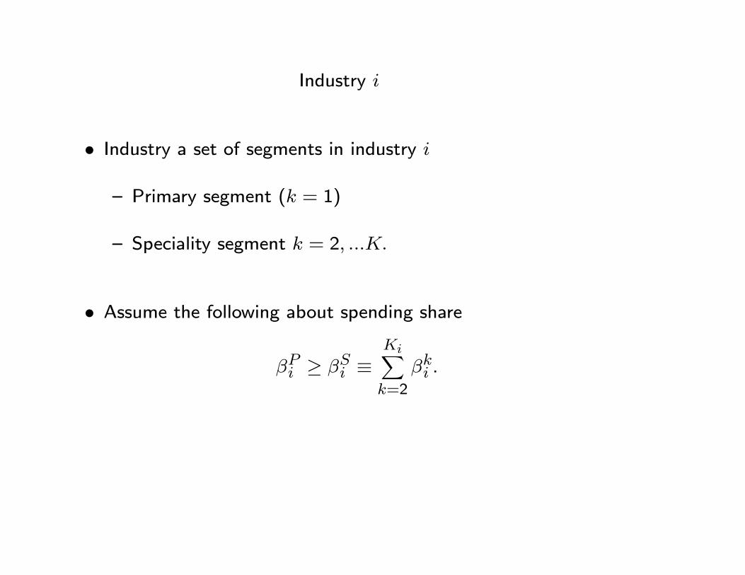
Industry

• Industry a set of segments in industry

— Primary segment ( = 1)

— Speciality segment = 2

• Assume the following about spending share

≥ ≡X=2

.

Model 1 of Speciality Segment: High Transportation Cost

• Parameters of speciality the same as primary EXCEPT spend-ing share of transportation cost (and variety)

() = 1 (),

• Parameter magnifies transportation cost

• Introduce internal geography at each location. Let be

land area.

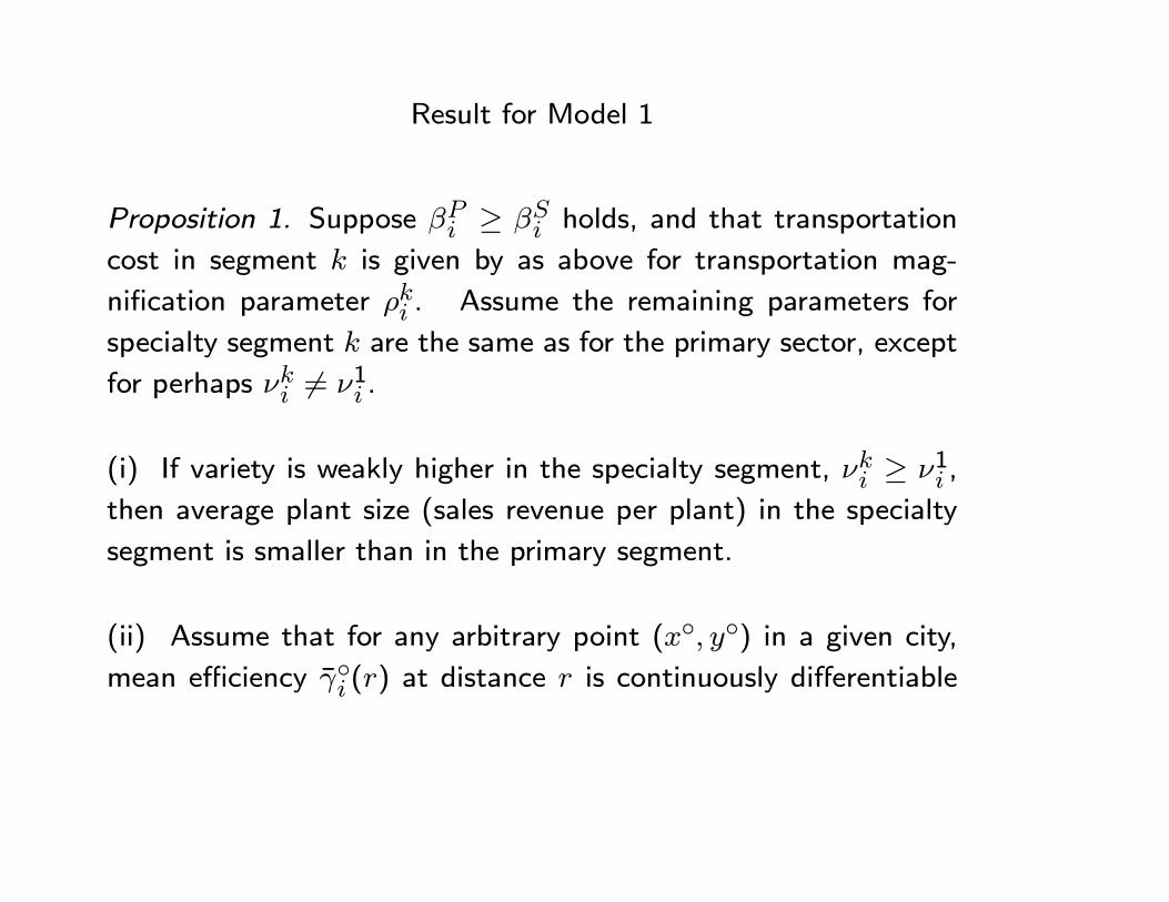
Result for Model 1

Proposition 1. Suppose ≥ holds, and that transportation

cost in segment is given by as above for transportation mag-

nification parameter . Assume the remaining parameters for

specialty segment are the same as for the primary sector, except

for perhaps 6= 1 .

(i) If variety is weakly higher in the specialty segment, ≥ 1 ,

then average plant size (sales revenue per plant) in the specialty

segment is smaller than in the primary segment.

(ii) Assume that for any arbitrary point (◦ ◦) in a given city,mean efficiency ◦ () at distance is continuously differentiable

and strictly positive. Consider making large, while rescaling

variety in segment according to

=³

´2,for a constant . Then

lim→∞

=2

2 × , (1)

where is the measure of plant counts in segment in industry

at city .

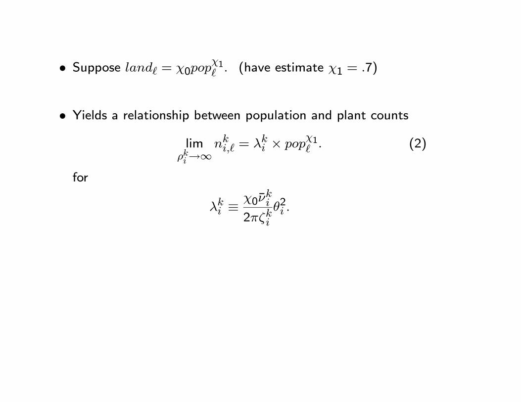
• Suppose = 01 . (have estimate 1 = 7)

• Yields a relationship between population and plant counts

lim→∞

= × 1 (2)

for

≡0

22 .

Model 2 of Speciality Segment: Niche with Idiosyncratic Sourcesof Supply

• Assume cost efficiency vector Γ = (1 2 ) for seg-ment ≥ 1 drawn from a distribution satisfying

⎛⎝ P0

0

⎞⎠ = P0 0

. (3)

• Suppose speciality segments in an industry, each has spend-ing share given by

=.

• Suppose for a given , variety in segment is equal to

=∗.

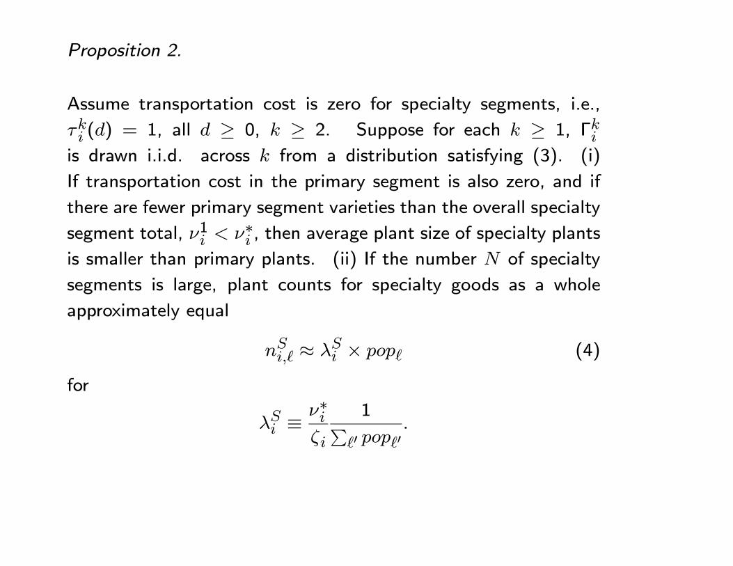
Proposition 2.

Assume transportation cost is zero for specialty segments, i.e.,

() = 1, all ≥ 0, ≥ 2. Suppose for each ≥ 1, Γis drawn i.i.d. across from a distribution satisfying (3). (i)

If transportation cost in the primary segment is also zero, and if

there are fewer primary segment varieties than the overall specialty

segment total, 1 ∗ , then average plant size of specialty plantsis smaller than primary plants. (ii) If the number of specialty

segments is large, plant counts for specialty goods as a whole

approximately equal

≈ × (4)

for

≡∗

1P0 0

.

Data

• 1997 Census of Manufactures (CM): Plant level data of theuniverse of plants (sales, location, etc.)

• 1997 Commodity Flow Survey (CFS): Sample of Shipments

from a sample of (15,000) plants

— origin and destination and link to CM

— after conditioning on industry and distance, we use 500,000

observations for structural estimates

Data Selections

• Industry defined at 6-digit NAICS level (North American In-dustry Classification System). Pick 172 (out of 473) indus-

tries where demand approximately follows population

• is population share

• Locations defined at level of Bureau of Economic AnalysisEconomic Area

— = 177

— Based on MSAs, except rural counties get included in the

partition

Seven Industries that Get Extra Attention

• 1997 changed from SIC to NAICS, a ”production based sys-tem.” Plants using the “same production technology” groupedin the same industry

• SIC system

— did this sometimes (sugar from beets and from cane dif-ferent industries)

— “missed” other times, some chocolate factories, wood fur-niture stores, etc. placed in retail under SIC

• 1997 micro data, for these seven industries for each planthave NAICS and SIC. Use this to classify plants as R or Mdepending on SIC. Take R as a proxy for speciality.

Table 2 Descriptive Statistics for the 1997 Reclassification Industries

by R and M Status NAICS Industry Classification

Classification Based on SIC

Number

of Plants

Mean Plant

Employ.

Export Share

Mean Location Quotient

Chocolate Candy R 440 8 .00 1.01 (NAICS 311330) M 421 70 .03 4.87

Nonchocolate Candy R 349 4 .00 1.01 (NAICS 311340) M 276 88 .03 4.61

Kitchen Cabinets R 2,055 5 .00 1.25 (NAICS 337110) M 5,908 15 .01 2.14 Upholstered Household Furniture R 576 5 .00 1.52 (NAICS 337121) M 1,130 77 .03 7.20 Wood Household Furniture R 815 6 .00 1.17 (NAICS 337122) M 3,035 41 .03 4.42

Quantitative Analysis

• Model of distance adjustment for ,

ln 0◦ = −loglog ln 0◦

which yields a constant distance elasticity loglog . The second

is a semi-log specification,

ln 0◦ = −semi,1 0◦ − semi,2 (0◦)

2 ,

• First-stage estimates: Constrained model with only primarysegment (one segment model)

— Pick and Γ = (1 2 177) to:

∗ fit sales distribution across locations perfectly (have theuniverse). Use iterative procedure to back out Γ.

∗ maximize conditional likelihood of the destinations in theshipment sample

∗ conditioned on ≥ 100 for shipments

Table 4 First Stage Results for the Seven Reclassification Industries

Reclassification Industries

LogLog Case

ConstantElasticity

Semi-Log

Case Elasticity

100 miles

Semi-Log

Case Elasticity

500 miles

LogLog Case

LogLike

Semi-Log

Case LogLike

Number of

Shipment Obs.

Chocolate Candy (311330) 0.31 0.06 0.37 -6947.0 -6842.8 1,633 Nonchocolate Candy (311340) 0.38 0.09 0.45

-10843.6

-10690.6 2,592

Curtains(314121) 0.69 0.23 0.90

-12917.9

-12864.0 3,068

Other Apparel (315999) 0.55 0.23 0.85

-17470.7

-17414.4 3,819

Kitchen Cabinets (337110) 1.16 0.41 1.62

-27046.6

-26767.7 6,655

Upholstered Household Furn.(337121) 1.19 0.36 1.47

-36714.7

-36439.6 8,837

Wood Household Furn.(337122) 0.67 0.22 0.84

-67889.5

-67746.4 15,624

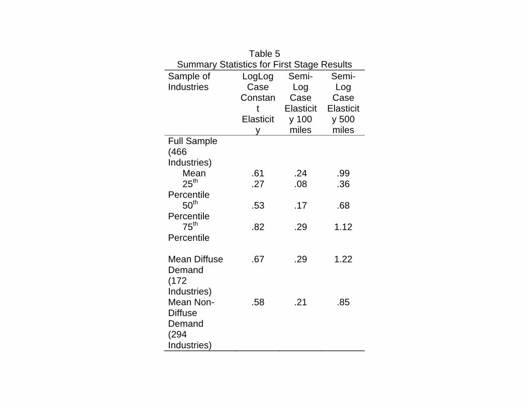
Table 5 Summary Statistics for First Stage Results

Sample of Industries

LogLog Case

Constant

Elasticity

Semi-Log

Case Elasticity 100 miles

Semi-Log

Case Elasticity 500 miles

Full Sample (466 Industries)

Mean .61 .24 .99 25th Percentile

.27 .08 .36

50th Percentile

.53 .17 .68

75th Percentile

.82 .29 1.12

Mean Diffuse Demand (172 Industries)

.67 .29 1.22

Mean Non-Diffuse Demand (294 Industries)

.58 .21 .85

• Stage 2: Estimate plant count model

— Baseline estimates, take limit where sales revenue share of

specialty is zero. So and Γ same as for one segment

model of just primary segment.

— Specialty segment still factors into plant counts. Pick and to fit

= (Γ

) + + + , (5)

— Also consider an alternative where make assumptions on

size of speciality plants and difference them out of sales,

with little difference in results.

Source: See

Table 6 Second-Stage Estimates of the Plant Count Parameters and Related Model and Data Statistics

Regression Results (s.e. in Parentheses)

Estimated Specialty

Count Share

(Percent)

Constantξ

Slope Speciality

λS

Slope Primary

λP

R2

Reclassification Industries Chocolate Candy (311330)

.4 (.2)

621.3 (52.3)

76.6 (13.0)

.69 80.8

Nonchocolate Candy (311340)

.1 (.1)

487.8 (31.2)

62.6 (7.9)

.79 80.4

Curtains(314121)

-.9 (.3)

2186.4 (56.4)

20.9 (8.1)

.92 97.1

Other Apparel (315999)

-1.8 (.4)

1287.0 (110.8)

287.0 (20.4)

.90 62.3

Kitchen Cabinets (337110)

1.5 (1.2)

5963.3 (230.5)

210.2 (21.5)

.89 78.4

Upholstered Household Furn. (337121)

-1.3 (.5)

975.5 (94.7)

270.3 (8.6)

.88 49.8

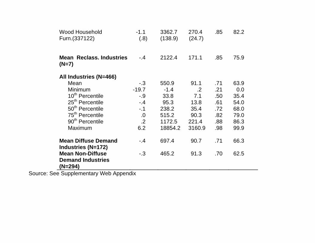
Wood Household Furn.(337122)

-1.1 (.8)

3362.7 (138.9)

270.4 (24.7)

.85 82.2

Mean Reclass. Industries (N=7)

-.4 2122.4 171.1 .85 75.9

All Industries (N=466) Mean -.3 550.9 91.1 .71 63.9 Minimum -19.7 -1.4 .2 .21 0.0 10th Percentile -.9 33.8 7.1 .50 35.4 25th Percentile -.4 95.3 13.8 .61 54.0 50th Percentile -.1 238.2 35.4 .72 68.0 75th Percentile .0 515.2 90.3 .82 79.0 90th Percentile .2 1172.5 221.4 .88 86.3 Maximum 6.2 18854.2 3160.9 .98 99.9 Mean Diffuse Demand Industries (N=172)

-.4 697.4 90.7 .71 66.3

Mean Non-Diffuse Demand Industries (N=294)

-.3 465.2 91.3 .70 62.5

Source: See Supplementary Web Appendix

Plan

• Compare

— Estimated industry model with only primary segment

— Estimated industry modwl with specialty segment

• Examine plant size/geographic concentration relationship

• Examine effect of China surge

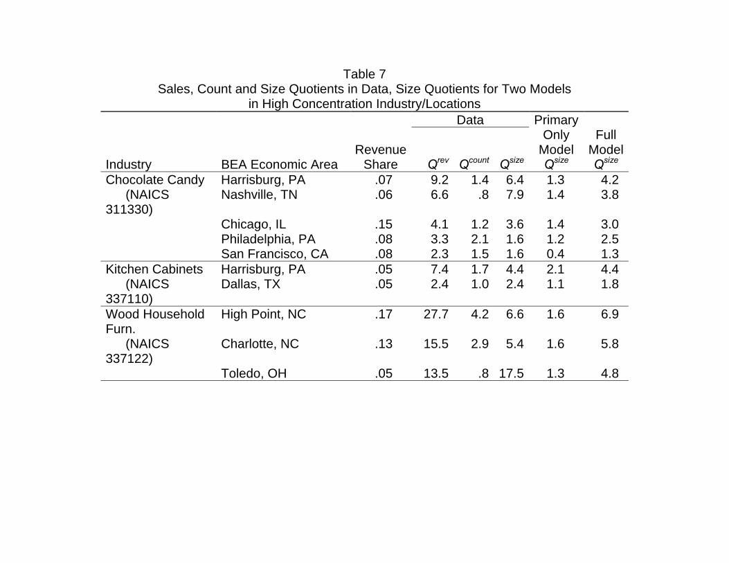
Table 7 Sales, Count and Size Quotients in Data, Size Quotients for Two Models

in High Concentration Industry/Locations

Industry BEA Economic Area Revenue

Share

Data PrimaryOnly

Model Qsize

Full ModelQsize Qrev Qcount Qsize

Chocolate Candy Harrisburg, PA .07 9.2 1.4 6.4 1.3 4.2 (NAICS 311330)

Nashville, TN .06 6.6 .8 7.9 1.4 3.8

Chicago, IL .15 4.1 1.2 3.6 1.4 3.0 Philadelphia, PA .08 3.3 2.1 1.6 1.2 2.5 San Francisco, CA .08 2.3 1.5 1.6 0.4 1.3 Kitchen Cabinets Harrisburg, PA .05 7.4 1.7 4.4 2.1 4.4 (NAICS 337110)

Dallas, TX .05 2.4 1.0 2.4 1.1 1.8

Wood Household Furn.

High Point, NC .17 27.7 4.2 6.6 1.6 6.9

(NAICS 337122)

Charlotte, NC .13 15.5 2.9 5.4 1.6 5.8

Toledo, OH .05 13.5 .8 17.5 1.3 4.8

Summary Statistics

Reclass.Industries (N=7 Industries)

N = 23 Industry/Locations Mean .11 14.0 4.3 5.4 1.4 3.9

Median .08 7.6 1.5 4.5 1.4 3.2All Industries (N = 466 Industries)

N=1708 Industry/Locations Mean

.11

17.6 6.5 4.4

1.2 3.0

Median .09 9.4 3.2 2.4 1.1 2.4Diffuse Demand Industries

N=589 Industry/Locations Mean

.11

18.2 5.8 5.3

1.2 3.2

(N = 172 Industries)

Median .09 9.2 2.8 2.6 1.2 2.6

Non-Diffuse Demand Industries

N=1119 Industry/Locations Mean .11 17.2 6.9 3.9 1.2 2.8

(N = 294 Industries)

Median .08 9.6 3.4 2.2 1.1 2.4


Modeling China Surge

• Baseline: distribute imports across ports.

• Model growth in imports from China as a new source of supply.Solve for to match change in imports 1997-2007

=

P0=1

0

0P

0=1 0

0 +

P0=1

0

0

(6)

We calculate by taking the weighted aver-

age of (6) across all destinations . We start by plugging in

the estimated domestic cost-efficiency parameters 0 for

1997 into (6).

• Next let

= × ,

where is the share in the 2007 data of man-ufacturing imports from China going through customs at loca-tion . We solve for the scaler so that the implied

value of equals the China new-import sharefor industry .

• Stochastic transition of cost efficiency. To explicitly take intoaccount this force, we employ the following procedure. Westart with those 88 industries in the bottom category of Table8 for which the new China share is zero. We take make agrid of the cost efficiencies in 1997 and 2007 and estimate astochastic transition process for the cost efficiencies over thegrid. We then assume the same transition matrix applies forthe other industries, and run 10,000 different simulations, tak-ing averages over simulations for each location and industry.

Table 8 Summary Statistics for 6-Digit NAICS Industries Classified by New China Share Category

Count of Industries

Mean of New

China Share 1997-2007

Mean of New All-Country Share 1997-2007

Mean Industry

Employment Growth

1997-2007 (percent)

All Industries 465 8 12 -21 By New China Share Category (percent) 50 to 97 23 71 72 -75 25 to 50 23 35 38 -51 10 to 25 50 16 21 -29 5 to 10 38 7 14 -33 >0 to 5 243 1 7 -12 None* 88 0 1 -14

*There are 12 industries in which the new China share is negative. In all of these cases, the value is negligible. (The minimum is -.013 and the mean is -.003.) For these cases we truncate the new China share at zero. Analogously, we truncate the new all-country share at zero. There are 465 industries in this table rather than 466, because NAICS 339111, “Laboratory apparatus & furniture mfg” had no data for 2007 because the industry was discontinued and the plants were reassigned to other industries.

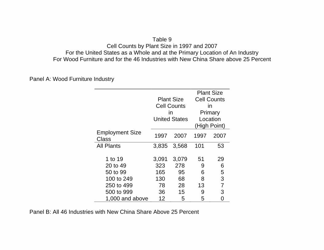
Table 9

Cell Counts by Plant Size in 1997 and 2007 For the United States as a Whole and at the Primary Location of An Industry

For Wood Furniture and for the 46 Industries with New China Share above 25 Percent

Panel A: Wood Furniture Industry

Plant Size Cell Counts

in United States


in Primary Location

(High Point) Employment Size Class 1997 2007 1997 2007

All Plants

3,835 3,568 101 53

1 to 19 3,091 3,079 51 29 20 to 49 323 278 9 6 50 to 99 165 95 6 5 100 to 249 130 68 8 3 250 to 499 78 28 13 7 500 to 999 36 15 9 3 1,000 and above 12 5 5 0

Panel B: All 46 Industries with New China Share Above 25 Percent


in United States


in Primary Location

Employment Size Class 1997 2007 1997 2007

All Plants

24,192 16,534 1,666 732

1 to 19 16,258 12,674 1,043 507 20 to 49 3,300 1,857 261 97 50 to 99 1,865 891 121 50 100 to 249 1,601 712 106 38 250 to 499 654 248 57 25 500 to 999 344 94 39 8 1,000 and above 170 58 39 7

Source: The cell counts are based on public tabulations from the Census discussed in Appendix B. The High Point, NC Area consists of the BEA Economic Area containing High Point, NC (consisting of 22 counties). For each industry, the Primary Location is the Economic Area with the highest sales revenue location quotient, among locations with at least 5 percent of U.S. sales.

Table 10 Actual Values in Data for High Concentration Industry/Cities Size and Count Quotients and Change in Count Quotients

Means Across New China Share Categories

Number of High

Concen. Industry/

Cities

Qsize

1997

Qcount

1997

Qcount

2007

Percent Change in

Count Shares

1997-2007 All 1703 4.4 6.5 5.5 -10 By New China Share Category (percent)

50 to 97 92 5.7 4.8 2.6 -37 25 to 50 101 4.5 3.8 2.8 -20 10 to 25 179 4.2 5.8 5.1 -5 5 to 10 130 5.0 5.0 4.4 -9 >0 to 5 890 4.1 7.7 6.7 -6 None 311 4.6 5.6 4.6 -10


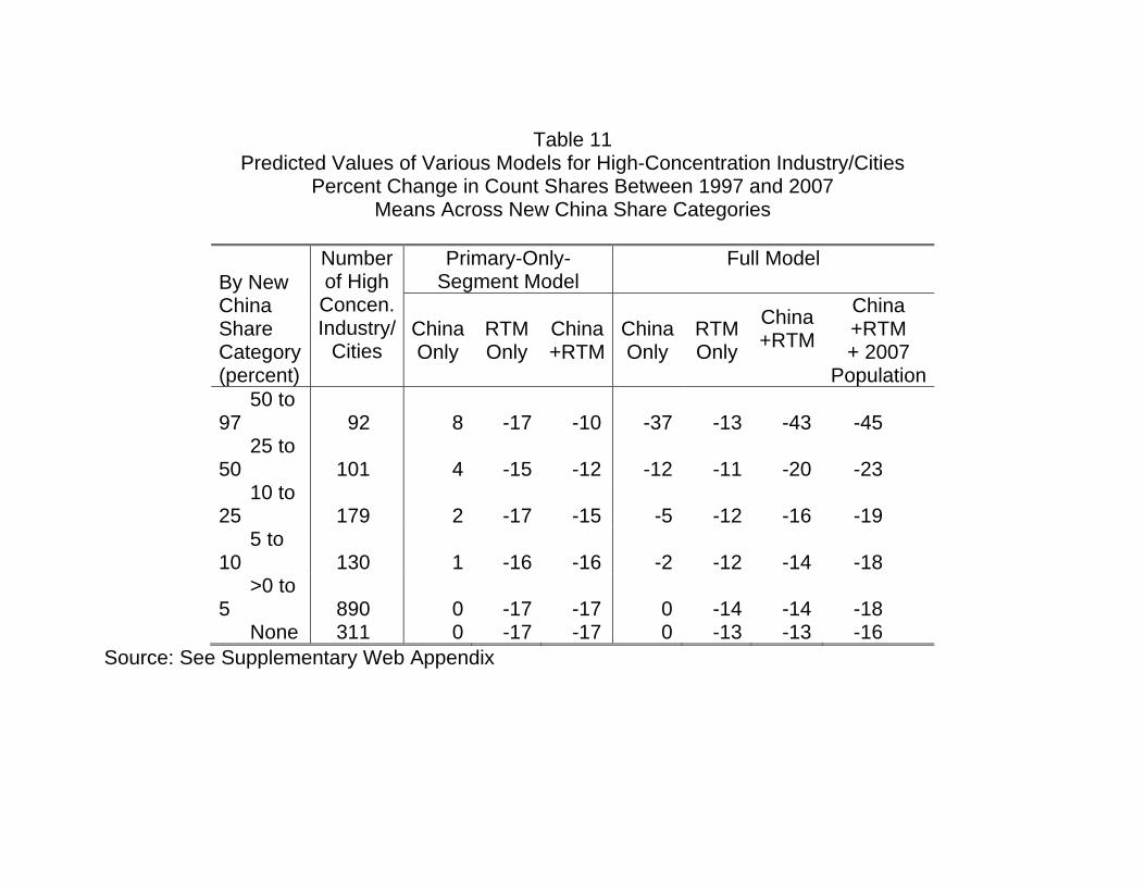
Table 11

Predicted Values of Various Models for High-Concentration Industry/Cities Percent Change in Count Shares Between 1997 and 2007

Means Across New China Share Categories

By New China Share Category (percent)

Number of High Concen.Industry/

Cities

Primary-Only-Segment Model

Full Model

China Only

RTM Only

China+RTM

China Only

RTM Only

China+RTM

China +RTM + 2007

Population 50 to 97 92 8 -17 -10 -37 -13 -43 -45 25 to 50 101 4 -15 -12 -12 -11 -20 -23 10 to 25 179 2 -17 -15 -5 -12 -16 -19 5 to 10 130 1 -16 -16 -2 -12 -14 -18 >0 to 5 890 0 -17 -17 0 -14 -14 -18 None 311 0 -17 -17 0 -13 -13 -16


Table 12 Estimated Primary Segment Plant Count Share for 1997 and 2007

By New China Share Categories

New China Share

Category (percent)

Total Establishment Count

(1,000 plants)

Estimated Primary Segment

Count Share (percent)

Change in Percent Primary

1997 2007 1997 2007 50 to 97 10 5 32 25 -6 25 to 50 15 11 27 16 -11 10 to 25 34 30 31 31 1 5 to 10 24 20 30 32 2 >0 to 5 156 153 34 33 -1 None 108 95 32 37 6


bernard, eaton, jensen kortum (bejk) -...

Documents