Technical Note: An Eaton and Kortum(2002) Model of Urbanization andStructural Transformation�

Guy MichaelsLondon School of Economics, CEP and CEPR

Ferdinand RauchLondon School of Economics and CEP

Stephen J. ReddingPrinceton University, NBER and CEPR

August 22, 2011

1 Introduction

This technical note extends the model of Michaels et al. (2011) to introduce Eaton and

Kortum (2002) heterogeneity within each sector, which facilitates a tractable analysis of

bilateral transport costs. We show how the resulting model can be calibrated using data on

employment by sector and location to determine productivity in each sector and location.

We undertake this calibration for each year separately without imposing prior structure

on the pattern of productivity growth over time. We show that the resulting calibrated

productivities support the explanation for the stylized facts in Michaels et al. (2011) based

on a combination of aggregate reallocation from agriculture to non-agriculture and di¤erences

in mean reversion in productivity between the two sectors.

2 Model

We consider an economy that features many locations indexed by i = 1; : : : ; I, labor and

land as factors of production, and agricultural and non-agricultural sectors denoted by K 2�This technical note provides additional supplementary material for Michaels, Redding and Rauch (2011)

�Urbanization and Structural Transformation,�London School of Economics, mimeograph.

1

fA;Ng. While locations can di¤er from one another in terms of both their productivities andbilateral transport costs, the model remains tractable because of the stochastic formulation

of productivity, which follows Eaton and Kortum (2002).

The economy as a whole is endowed with a measure Lt of workers, who are mobile

across locations and are each endowed with one unit of labor that is supplied inelastically

with zero disutility.1 Employment varies across sectors and locations because of exogenous

productivity di¤erences. Population mobility ensures that workers in all populated locations

receive the same real income in equilibrium.

Each location is endowed with a �xed measure Hi of land, which can be used residentially

or commercially in agriculture and non-agriculture. Production in each location can be either

completely specialized in one sector or incompletely specialized. Land in each location is

owned by immobile landlords, who earn rents and consume with the same preferences as

workers.

There are two key di¤erences between the sectors in the model. First, we make the

natural assumption that agriculture is more land intensive than non-agriculture. Second, we

allow the two sectors to di¤er in terms of their distribution of productivities across locations.

Together, these two features of the model allow the share of agriculture in employment to vary

with population density. While our focus on agriculture and non-agriculture is motivated

by our empirical �ndings of the importance of reallocation away from agriculture, the model

could be extended to disaggregate non-agriculture into manufacturing and services.

The model captures the two main explanations for an aggregate reallocation of employ-

ment away from agriculture in the macroeconomics literature: (a) more rapid productivity

growth in agriculture than in non-agriculture combined with inelastic demand across sectors

and/or (b) non-homothetic preferences combined with a rise in real income that leads to a

change in the relative weight of sectors in consumer preferences. Either of these explana-

tions can induce an aggregate reallocation of employment away from agriculture, and our

objective is not to distinguish between them, but rather to examine the implications of such

an aggregate reallocation for the distribution of population across locations.

1Since labor force participation is not strongly related to population density in our data, the modelabstracts from workers� labor force participation decision and assumes that total employment is equal tototal population. While the analysis could be extended to allow each worker to have a �xed number ofdependents, who consume but do not work, this would complicate the analysis without adding much insight.

2

2.1 Consumer Preferences

Preferences are de�ned over goods consumption (Cjt) and residential land use (HUjt) and

are assumed for simplicity to take the Cobb-Douglas form:2

Ujt = �jtC�jtH

1��Ujt ; 0 < � < 1; (1)

where �jt captures residential consumption amenities in location j at time t.3

The goods consumption index is de�ned over consumption of agriculture (CAjt) and non-

agriculture (CNjt):

Cjt =� AtC

�Ajt + NtC

�Njt

� 1� ; 0 < � =

1

1� �< 1; At; Nt > 0; (2)

where agriculture and non-agriculture are assumed to be complements (0 < � < 1), which

implies inelastic demand between the two goods.4

The demand parameters ( At, Nt) capture the relative strength of consumer tastes

for each good and may be a function of the common value of real income (vt) across all

locations ( At = A (vt), Nt = N (vt)), as in the non-homothetic speci�cation of CES

utility considered by Sato (1977).5 Under our assumption of CES preferences, changes

in relative productivity across sectors are isomorphic to changes in the relative weight of

sectors in consumer preferences, in the sense that they have the same e¤ects on equilibrium

expenditure and employment shares. Since real income is the same across locations in an

equilibrium characterized by population mobility, the demand weights At = A (vt) and

Nt = N (vt) are common across locations, which enables us to determine an idiosyncratic

component of productivity that varies across locations within each sector. However, the

common demand weights At = A (vt) and Nt = N (vt) cannot be separately identi�ed

from aggregate di¤erences in productivity across sectors using the employment data available

to us. Therefore we normalize the demand weights to one ( At = A = 1 and Nt = N = 1

for all t), so that the calibrated aggregate component of productivity in each sector captures

both the common demand weights and aggregate productivity.

2For empirical evidence using U.S. data in support of the constant housing expenditure share implied bythe Cobb-Douglas functional form, see Davis and Ortalo-Magne (2008).

3To simplify the exposition, throughout the following, we denote producing locations by i and consuminglocations by j.

4In assuming inelastic demand between agriculture and non-agriculture, we follow a large literature inmacroeconomics, as discussed in Ngai and Pissarides (2007).

5The relative weight of the two sectors in consumer preferences ( At, Nt) may also capture di¤erencesin product quality across sectors and over time.

3

The goods consumption index for each sector K in location j at time t is de�ned over

consumption (cKjt (h)) of a �xed continuum of products h 2 [0; 1] (e.g. rice, wheat, corn etcfor agriculture):6

CKjt =

�Z 1

0

cKjt (h)� dh

� 1�

; � =1

1� �> 1; K 2 fA;Ng ; (3)

where we make the plausible assumption that products within a given sector are substitutes

for one another (� > 1). While for simplicity we assume the same elasticity of substitution

in both sectors, it is straightforward to relax this assumption.

2.2 Production

Production in each sector is modeled following Eaton and Kortum (2002), which we augment

to introduce land as an additional factor of production and labor mobility across locations.7

Each location i draws an idiosyncratic productivity (zK (h)) for each product h within each

sector K. Productivity is independently drawn across products, sectors and time from a

Fréchet distribution:

FKit (zK) = e�TKitz��KK ; K 2 fA;Ng ; (4)

where the scale parameter TKit determines average productivity for each sector-location-

year; the shape parameter �K controls the dispersion of productivity across products within

each sector-location-year. Variation in the productivity parameter (TKit) across sectors and

locations determines the distribution of employment across locations within each sector and

the distribution of population across locations.

Products within each sector are produced under conditions of perfect competition using

labor and land according to a Cobb-Douglas production technology.8 Output can be traded

across locations subject to iceberg variable trade costs, where dKji > 1 units of a product

6We use �sector�or �good�to refer to the broad categories of agriculture and non-agriculture and reserve�product�for the various types of good within each sector (e.g. rice and wheat within agriculture).

7While Yi and Zhang (2010) distinguish between agriculture and non-agriculture in a model of the ag-gregate economy following Eaton and Kortum (2002), we introduce population mobility and endogenousland use across many disaggregate regions within an economy. While Holmes, Hsu and Lee (2011) developa two-region version of Bernard, Eaton, Jensen and Kortum (2003) to analyze endogenous innovation andlocation decisions, we distinguish between agriculture and non-agriculture and examine the implications ofstructural transformation for urbanization.

8While we assume a Cobb-Douglas production technology and follow a long line of research in macro-economics in focusing on changes in aggregate productivity or relative demand across sectors as the sourcesof reallocation, another potential explanation for this reallocation involves distinguishing between land andlabor-augmenting technological change using a more �exible production technology.

4

in sector K must be shipped from location i in order for one unit to arrive in location j.

Therefore the cost to a consumer in location j of purchasing one unit of a product h within

sector K from location i is as follows:

pKjit (h) =w�Kit r

1��Kit dKji

zKit (h); 0 < �K < 1; K 2 fA;Ng ; (5)

dKji = � ji�K ; �K > 0;

where wit and rit denote the wage and land rent, respectively, in location i at time t.

We assume that agriculture is land intensive relative to non-agriculture (�A < �N), which

together with sectoral di¤erences in the pattern of calibrated productivities (TKit) across

locations rationalizes sectoral di¤erences in the pattern of employment across locations as

an equilibrium of the model. We follow a long gravity equation literature in assuming that

bilateral trade costs are a log linear function of bilateral distance (� ji), where the distance

coe¢ cient �K parameterizes the elasticity of trade costs with respect to distance. In our

calibration of the model, we examine the extent to which observed changes in employment

can be explained simply by di¤erences in aggregate growth rates and mean reversion of

productivity across sectors. Therefore, consistent with empirical �ndings in the gravity

equation literature, we assume that the distance coe¢ cient is constant over time.9

2.3 Expenditure Shares

Given the above speci�cation of preferences and technology, consumer equilibrium can be

characterized by �rst determining shares of expenditure across locations within each sector,

and next determining shares of expenditure across sectors.

Price distributions: Before determining expenditure shares, we provide a character-

ization of the distribution of prices, which follows Eaton and Kortum (2002). Note that a

given product is homogeneous in the sense that one unit of that product is the same as any

other unit of that product. Therefore the representative consumer in a given location sources

each product from the lowest-cost supplier to that location:

pKjt (h) = min fpKjit (h) ; i = 1; : : : ; Ig ; K 2 fA;Ng : (6)

9While the level of trade costs has fallen over time, the empirical gravity equation literature �nds that theelasticity of trade costs with respect to distance has remained remarkably constant over time, as surveyed inDisdier and Head (2008). Since we calibrate the model for each year separately, it would be straightforwardto relax the assumption of constant �K .

5

Using the pricing rule (5) and the Fréchet distribution of productivities (4), the distribution

of prices within a sector K faced by the representative consumer in location j for goods

sourced from location i is:

GKjit(pK) = Pr[pKjit � pK ] = 1� FKit

w�Kit r

1��Kit dKjipK

!;

GKjit(pK) = 1� e�TKit(w�Kit r

1��Kit dKji)

��Kp�KK ; K 2 fA;Ng : (7)

Since goods are sourced from the lowest-cost supplier (6), the distribution of prices within

sector K in location j for goods actually purchased is:

GKjt (pK) = 1�IYi=1

[1�GKjit(pK)] = 1� e��Kjtp�KK ; (8)

�Kjt �IXs=1

TKst

�w�Kst r

1��Kst dKjs

���K; K 2 fA;Ng ; (9)

where the distribution of prices within sector K in location j for goods actually purchased

(GKjt (pK)) depends on the productivity parameter (TKit) for each location, which we cali-

brate based on the observed employment data, as discussed below.

Expenditure shares across locations: Since goods are sourced from the lowest-cost

supplier (6), the probability that location j sources a product h within sectorK from location

i is:

�Kjit = Pr [pKjit (h) � min fpKjst (h)g ; s 6= i;K 2 fA;Ng]

=

Z 1

0

Ys 6=i

[1�GKjst (pK)] dGKjit (pK) :

Using the bilateral price distribution (7), the probability that location j sources a product

h from location i within sector K can be expressed as:

�Kjit (wt; rt;TKt;dK) =TKit

�w�Kit r

1��Kit dKji

���KIXs=1

TKst

�w�Kst r

1��Kst dKjs

���K ; K 2 fA;Ng ; (10)

where bold math font is used to denote a vector or matrix, so that TKt is the vector of

productivities across locations in sector K and dK is the matrix of bilateral trade costs

between locations for sector K.

6

Following Eaton and Kortum (2002), another implication of the Fréchet distribution of

productivities is that the distribution of prices in a given location j for products actually

sourced from another location i is independent of the identity of the location i and equal to

the distribution of prices in location j. To derive this result, note that the distribution of

prices in location j conditional on sourcing products from location i is:

1

�Kjit

Z pK

0

Ys 6=i

[1�GKjst (q)] dGKjit (q) = 1� e��Kjtp�KK = GKjt (pK) ;

where we have used the bilateral and multilateral price distributions, (7) and (8) respectively.

Intuitively, under the assumption of a Fréchet productivity distribution, a source location

i with a higher scale parameter (TKit), and hence a higher average productivity, expands

on the extensive margin of the number of products supplied exactly to the point at which

the distribution of prices for the products it actually sells in destination j is the same as

destination j�s overall price distribution.

Since the distribution of prices in location j for goods actually purchased is the same

across all source locations i, it follows that the share of location j�s expenditure within

sector K on products sourced from another location i is equal to the probability of sourcing

a product from that location (�Kjit). Therefore the share of location j�s expenditure within

sector K on products sourced from another location i is given by (10).

Expenditure shares across sectors: Using the CES goods consumption index (2),

the share of location j�s expenditure on goods consumption that is allocated to sector K

depends on the dual price index for each sector (PKjt) as follows:

�Kjt = �KP

1��Kjt

�AP1��Ajt + �NP

1��Njt

; K 2 fA;Ng ; (11)

where inelastic demand between agriculture and non-agriculture (0 < � < 1) implies that a

sector�s share of goods consumption expenditure is increasing in its relative price index.

Following Eaton and Kortum (2002), the dual price index for each sector (PKjt) can be

determined using the multilateral distribution of prices (8):

PKjt =

�Z 1

0

pKjt (h)1�� dh

� 11��

; K 2 fA;Ng ;

=

�Z 1

0

p1��KjtdGKjt (pK)

� 11��

;

=

�Z 1

0

�K�Kjtp�K��Kjt e��Kjtp

�KKjtdpKjt

� 11��

:

7

Using the following change of variable:

xKjt = �Kjtp�KKjt;

) pKjt =

�xKjt�Kjt

� 1�K

; dpKjt =1

�K

�xKjt�Kjt

� 1��K�K 1

�KjtdxKjt;

we obtain:

PKjt = ��1=�KKjt

�Z 1

0

x(1��)=�KKjt e�xKjtdxKjt

� 11��

;

which implies:

PKjt = K��1=�KKjt = K

"IXs=1

TKst

�w�Kst r

1��Kst dKjs

���K#�1=�K; K 2 fA;Ng ; (12)

where K ���

��K + 1� �

�K

�� 11��

;

where � (�) is the gamma function.Having determined the dual price index for each sector (PKjt), the dual price index for

the aggregate goods consumption index (2) follows immediately:

Pjt =� �AP

1��Ajt + �NP

1��Njt

� 11�� ; (13)

Combining the sectoral expenditure share (11) with the sectoral price index (12), the share of

location j�s expenditure on goods consumption that is allocated to sector K can be written

solely in terms of trade costs, wages, rents and productivities in all locations:

�Kjt (wt; rt;TAt;TNt;dK) =

�K 1��K

"IXs=1

TKst

�w�Kst r

1��Kst dKjs

���K#� 1���K

PZ2fA;Ng

�Z 1��Z

"IXs=1

TZst

�w�Zst r

1��Zst dZjs

���Z#� 1���Z

: (14)

2.4 Factor Markets

Land market clearing in each location implies that total land income equals the sum of pay-

ments to residential land plus payments to land used in production in each sector. With a

Cobb-Douglas upper tier of utility, a constant fraction of total income is spent on residential

land. Additionally, with a Cobb-Douglas production technology, payments to land in each

8

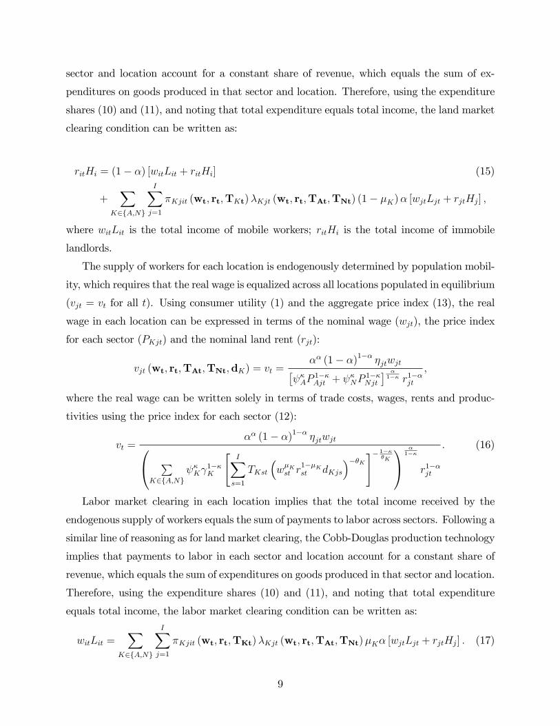
sector and location account for a constant share of revenue, which equals the sum of ex-

penditures on goods produced in that sector and location. Therefore, using the expenditure

shares (10) and (11), and noting that total expenditure equals total income, the land market

clearing condition can be written as:

ritHi = (1� �) [witLit + ritHi] (15)

+X

K2fA;Ng

IXj=1

�Kjit (wt; rt;TKt)�Kjt (wt; rt;TAt;TNt) (1� �K)� [wjtLjt + rjtHj] ;

where witLit is the total income of mobile workers; ritHi is the total income of immobile

landlords.

The supply of workers for each location is endogenously determined by population mobil-

ity, which requires that the real wage is equalized across all locations populated in equilibrium

(vjt = vt for all t). Using consumer utility (1) and the aggregate price index (13), the real

wage in each location can be expressed in terms of the nominal wage (wjt), the price index

for each sector (PKjt) and the nominal land rent (rjt):

vjt (wt; rt;TAt;TNt;dK) = vt =�� (1� �)1�� �jtwjt�

�AP1��Ajt + �NP

1��Njt

� �1�� r1��jt

;

where the real wage can be written solely in terms of trade costs, wages, rents and produc-

tivities using the price index for each sector (12):

vt =�� (1� �)1�� �jtwjt0@ P

K2fA;Ng �K

1��K

"IXs=1

TKst

�w�Kst r

1��Kst dKjs

���K#� 1���K

1A�1��

r1��jt

: (16)

Labor market clearing in each location implies that the total income received by the

endogenous supply of workers equals the sum of payments to labor across sectors. Following a

similar line of reasoning as for land market clearing, the Cobb-Douglas production technology

implies that payments to labor in each sector and location account for a constant share of

revenue, which equals the sum of expenditures on goods produced in that sector and location.

Therefore, using the expenditure shares (10) and (11), and noting that total expenditure

equals total income, the labor market clearing condition can be written as:

witLit =X

K2fA;Ng

IXj=1

�Kjit (wt; rt;TKt)�Kjt (wt; rt;TAt;TNt)�K� [wjtLjt + rjtHj] : (17)

9

2.5 General Equilibrium

Given productivity in each sector and location {TAit; TNit}, the model can be solved by

determining wages, rents and labor supplies for each location {wit, rit, Lit}, which can be

used to determine all other endogenous variables of the model, including employment for each

sector and location {LAit, LNit}. The equilibrium vector of wages, rents and labor supplies is

determined by the system of three equations for all locations given by labor market clearing

(17), land market clearing (15) and population mobility (16).

In our quantitative analysis, rather than solving for the equilibrium vector given produc-

tivity, we instead assume that observed employment in each sector and location {LAit, LNit}

is an equilibrium of the model and calibrate the productivity in each sector and location

{TAit; TNit} required to support observed employment as an equilibrium. In addition to de-

termining productivity, the calibration also yields solutions for wages, rents and the other

endogenous variables of the model.

2.6 Model Calibration

The calibration of the model uses the expressions for labor payments in each sector from the

labor market clearing condition (17), the land market clearing condition (15), the population

mobility condition (16), observed employment in each sector and location, land area and

bilateral distance {LAit, LNit, Hi, � ij}, to calibrate unobserved productivity in each sector

and location {TAit, TNit}.

The remainder of this section proceeds as follows. In Subsection 2.6.1, we solve for land

rents in terms of wages and observables. In Subsection 2.6.2, we use the expression for labor

payments in each sector to derive a �rst relationship between productivity in each sector and

wages. In Subsection 2.6.3, we use population mobility across locations to derive a second

relationship between wages and productivity in each sector. In Subsection 2.6.4, we discuss

how these two relationships can be used to calibrate unobserved productivity for each sector

and location {TAit, TNit}.

2.6.1 Land Rents

We begin by combining labor payments in each sector and land market clearing to obtain

an expression for land rents in terms of wages and observables. Note that labor payments

in a given sector and location account for a constant fraction of revenue, which equals total

10

expenditure on goods produced in that sector and location. Using the Cobb-Douglas upper

tier of utility, the share of goods consumption expenditure allocated to each sector (�Kit),

the share of sectoral expenditure allocated to each location (�Kjit), and the Cobb-Douglas

production technology, labor payments in a given sector and location can be written as:

witLKit =IXi=1

�Kjit (wt; rt;TKt;dK)�Kjt (wt; rt;TAt;TNt;dK)�K� [wjtLjt + rjtHj] ; (18)

where bold math font again denotes a vector.

Using this expression for labor payments in the land market clearing condition (15), land

rents (rit) can be solved for as a function of observed employment (LAit and LNit), observed

land area (Hi), wages (wit) and parameters:

rit = #itwit; #it �1

�

LitHi

�(1� �) +

�1� �A�A

�LAitLit

+

�1� �N�N

�LNitLit

�; (19)

where Lit = LAit + LNit. In this expression, the relative value of rents and wages (#it) is

pinned down by parameters and observed data {LAit, LNit, Hi}.

Therefore, equilibrium relative factor prices (rit=wit) depend through #it on the share of

residential land in consumer expenditure (1 � �), the observed ratio of total employment

to land area (Lit=Hi), factor intensities in each sector (�K), and the observed share of each

sector in total employment (LKit=Lit).

2.6.2 Labor Payments

Having solved for land rents as a function of wages, we now show how labor payments for

each sector can be used to determine productivity in each sector given wages. Substituting

for land rents (rit) using (19), payments to labor (18) in each sector and location can be

written as the following implicit function:

�Kit = witLKit�IXj=1

�Kjit (wt;#t;TKt;dK)�Kjt (wt;#t;TAt;TNt;dK)�K�wjt [Ljt + #jtHj] = 0;

(20)

where #t is determined by observables.

Proposition 1 Given observed employment (LKit), land area (Hi) and bilateral distance (� ji

and hence dKji) and assumed values of wages (wit), there exists a unique (normalized) value

for calibrated productivity for each sector and location (TKit) that solves the labor payments

condition (20) for each sector and location.

11

Proof. See Subsection 2.9 of this web appendix.

Intuitively, for given assumed values of wages, observed employment for each sector and

location determines the value that productivity must take for each sector and location in an

equilibrium where the total value of labor demand equals the total value of labor supply.

2.6.3 Population Mobility

We now derive another relationship between wages and productivity from the population

mobility condition, which requires workers to receive the same equilibrium real income across

all populated locations. Substituting for land rents (rit) using (19), the population mobility

condition (16) can be re-written as the following implicit function:

it =

��� (1� �)1�� �jt

�1=�wjt0@ P

K2fA;Ng �K

1��K

"IXs=1

TKst

�wst#

1��Kst dKjs

���K#� 1���K

1A1

1��

#(1��)=�jt

���� (1� �)1�� �it

�1=�wit0@ P

K2fA;Ng �K

1��K

"IXs=1

TKst

�wst#

1��Kst dKis

���K#� 1���K

1A1

1��

#(1��)=�it

= 0; (21)

for all populated locations i and j, where #it is determined by observables.

Proposition 2 Given observed employment (LKit), land area (Hi) and bilateral distance

(� ji and hence dKji) and assumed values of productivities (TAit, TNit), there exists a unique

(normalized) wage for each location (wit) that solves the population mobility condition (21)

for each sector and location.

Proof. See Subsection 2.10 at the end of this appendix.

Intuitively, real wages in each location depend on wages, consumer prices and rents.

But rents can be solved for as a function of wages and observables, which in turn implies

that consumer price indices can be determined as a function of wages and productivities.

Therefore, given assumed values of productivities in each sector and location, we can solve

for the unique values of wages for each location for which real wages are equalized.

12

2.6.4 Productivity and Wages

The calibration of the model is fully described by the labor payments condition (20) for the

two sectors and the population mobility condition (21). Together these provide a system of

three equations for each location that determines productivity for the two sectors and wages

for each location {TAit, TNit, wit}, given observed employment in each sector and location,

land area and distance.

To calibrate the model, we �rst assume values of wages for each location and use the

labor payments condition (20) for the two sectors to determine unique values of productivity

for each sector and location {TAit, TNit}. We next use these calibrated productivities and

the population mobility condition (21) to determine unique values of wages for each location

{wit}. If these solutions for wages di¤er from the assumed values for wages used to calibrate

productivity, we update the assumed values of wages and re-calibrate productivities for each

sector and location. We repeat this process until the solutions for wages from the population

mobility condition equal the assumed values of wages used in the labor payments conditions.

For di¤erent initial assumed values of wages, we �nd that the system of equations given

by the labor payments and population mobility conditions (20)-(21) converges to a unique

equilibrium. Using the resulting solutions for equilibrium wages and productivity in the two

sectors {wjt, TAjt, TNjt}, all other endogenous variables of the model can be determined.

From the labor payments and population mobility conditions (20)-(21), di¤erences in

consumption amenities {�it} across locations have similar e¤ects on equilibrium wages as

di¤erences in productivities {TAit, TNit} across locations that are common to both sectors.10

Therefore we normalize �� (1� �)1�� �it = 1, so that di¤erences in consumption amenities

across locations are captured in the calibrated productivities.

The labor payments conditions for the two sectors (20) are homogeneous of degree zero in

productivities {TAit, TNit}, which re�ects the fact that in general equilibrium the distribution

of employment across sectors and locations depends on relative rather than absolute levels of

productivity. To calibrate productivity, we impose the following two normalizations. First,

we decompose productivity in each sector K, location i and year t (TKit) into an aggregate

component that is common across locations (T SKt) and an idiosyncratic component that is

10In the presence of bilateral trade costs, higher productivity in a location reduces its consumer price indexand hence raises its indirect utility relative to other locations through the denominator in (21). In contrast,greater consumption amenities in a location raise its indirect utility relative to other locations through thenumerator in (21).

13

speci�c to each location (T IKit): TKit = T SKtTIKit. We normalize idiosyncratic productivity

to have a mean of one hundred across locations in each sector and year, 1I

PIi=1 T

IKit = 100

for K 2 fA;Ng. With this �rst normalization, T IKit captures a location�s productivity in asector and year relative to average productivity in that sector and year, while {T SAt, T

SNt}

capture average levels of relative productivity in the two sectors. Second, we normalize

aggregate productivity in non-agriculture to equal one hundred (T SNt = 100). With this

second normalization, T SAt captures aggregate productivity in agriculture relative to non-

agriculture in each year. Although the use of alternative normalizations results in di¤erent

absolute levels of productivities, it leaves relative productivities unchanged.11

2.7 Model Parameters

Our calibration of the model requires data on employment by sector and location, which

is not available for MCDs for intermediate years between 1880 and 2000. To examine the

timing of structural transformation across these intermediate years, we calibrate the model

using our counties dataset for twenty-year intervals from 1880-2000. To compare the results

of the model calibration with our baseline empirical �ndings in Michaels et al. (2011), we

concentrate on our baseline sample of the A and B states, which have a longer history of

settlement and hence are likely to be more closely approximated by the assumption that

observed employment is an equilibrium of the model. Nonetheless, we �nd a similar pattern

of results for the full sample of states.

We choose values for the model�s parameters based on central estimates from the existing

empirical literature. Using the estimates for the United States in Davis and Ortalo-Magne

(2008), we set of the share of residential land in consumer expenditure (1 � �) equal to

0:25. Following a large literature in macroeconomics, including Ngai and Pissarides (2007),

we assume inelastic demand between agriculture and non-agriculture, and set the elasticity

of substitution across the two sectors (�) equal to 0:5. Within each sector, we assume that

di¤erent products are substitutes for one another and set the elasticity of substitution within

sectors (�) equal to 4, which is comparable to the empirical estimate for U.S. manufacturing

plants of 3:8 in Bernard, Eaton, Jensen and Kortum (2003).

11Although improvements in productivity that are common across sectors and locations leave the distri-bution of employment across sectors and locations unchanged, they do increase indirect utility. Under ourtwo normalizations, the common absolute level of productivity across sectors and locations is captured inthe common level of indirect utility across all locations (vt).

14

To focus on di¤erences in average productivity across sectors and locations (TAjt, TNjt),

we assume that the Fréchet shape parameter (�K) determining the dispersion of productivi-

ties is the same across sectors. Following the trade literature, we assume a value of �K equal

to 4, which is consistent with the estimates in Donaldson (2010), Eaton and Kortum (2002)

and Simonovska and Waugh (2011). For the elasticity of trade costs with respect to distance

(�K), we assume a value of 0:33, which is in line with the range of estimates in Limao and

Venables (2001) and Hummels (2007). Together the elasticity of trade costs with respect to

distance of 0.33 and the Fréchet shape parameter of 4 imply an elasticity of trade �ows with

respect to distance (��K�K) of �1:33, which is consistent with the empirical estimates fromthe gravity equation literature surveyed in Disdier and Head (2008). To measure transport

costs between pairs of counties, we use bilateral great circle distances between their centroids.

To measure the transport costs that a county incurs in serving itself, we follow the empiri-

cal economic geography literature in constructing a measure of a county�s internal distance.

Following Head and Mayer (2004) and Redding and Venables (2004), we approximate each

county with a circle that has the same area as the county and evaluate each county�s internal

distance as the average distance between pairs of points within that circle.

In the model, there is a one-to-one relationship between the shares of labor and land

in production costs and the shares of mobile and immobile factors in production costs.

In the data, the mapping from mobile and immobile factors to labor and land may be

imperfect, because there are additional factors of production other than labor and land (e.g.

physical capital), and because other factors of production besides land can exhibit a degree

of immobility across locations (e.g. buildings and structures). To determine the share of

immobile factors in production costs, we use the U.S. estimates from Table 5 of Valentinyi

and Herrendorf (2008). For non-agriculture, we set the share of immobile factors in costs

(1��N) equal to 0:18. For agriculture, we set the share of immobile factors in costs (1��A)equal to 0:22.

2.8 Quantitative Results

Our calibration of the model is undertaken for each year separately without imposing prior

structure on the pattern of productivity growth over time. In this subsection, we examine

whether the resulting calibrated productivities are consistent with our explanation for the

stylized facts based on aggregate reallocation and di¤erences in mean reversion across sectors.

15

Before examining the calibrated productivities, we present evidence on the pattern of

aggregate reallocation away from agriculture over time. In Panel A of Figure 1, we display

agriculture�s share of aggregate employment in our counties dataset for each year of our sam-

ple. As apparent from the �gure, there is a substantial aggregate reallocation of employment

away from agriculture, which decelerates from 1920-1940 (during the agricultural depression

of the 1920s and the Great Depression of the 1930s) and accelerates from 1940-1960 (in the

years surrounding the Second World War). These changes in the pace of aggregate realloca-

tion are also evident in Panel B of Figure 1, which shows the annualized proportional rate of

growth in agriculture�s share of employment for each twenty-year period. By the end of our

sample, the agricultural sector accounts for less than two percent of aggregate employment

(Panel A), but its small size is associated with large proportional rates of decline in its share

of aggregate employment (Panel B).

In Panel C of Figure 1, we show the annualized proportional rate of growth of calibrated

aggregate productivity in agriculture relative to non-agriculture for each twenty-year period

(� ln�T SAt=T

SNt

�). Care should be taken in interpreting these rates of growth of calibrated

relative aggregate productivity, because they are based on our normalization that the rela-

tive weight of sectors in demand is constant over time. Under this normalization, the rates

of growth of calibrated relative aggregate productivity capture both true di¤erences in ag-

gregate productivity growth across sectors and changes in the common relative weight of

sectors in demand (e.g. due to non-homothetic preferences or changes in product quality).

Despite these caveats, the �nding of faster aggregate productivity growth in agriculture than

in non-agriculture in Panel C is consistent with the results of empirical growth accounting

studies for the U.S. during our sample period, including Kuznets (1966) from 1870-1940

and Maddison (1980) from 1950-1976. Furthermore, these �ndings are also consistent with

the economic history literature on the development of U.S. agriculture, which emphasizes

the role of productivity-enhancing improvements in technology, such as mechanization and

biological innovation (see Cochrane 1979 and Rasmussen 1962).

The constant elasticity functional forms in the model imply that proportional changes

in relative aggregate productivity across sectors are associated with proportional changes

in the shares of sectors in aggregate employment. Therefore the pattern of relative aggre-

gate productivity growth in Panel C closely mirrors the pattern of proportional changes in

agriculture�s share of aggregate employment in Panel B. The relationship, however, is not

16

necessarily one-for-one, because the calibrated values of aggregate productivity depend on

the distribution of employment across sectors and locations with di¤erent idiosyncratic pro-

ductivities and bilateral transport costs. As a result, a given change in relative aggregate

productivity can be associated with di¤erent changes in agriculture�s share of aggregate em-

ployment depending on the pattern of idiosyncratic productivity growth and employment

across locations in each sector.

Our explanation for the stylized facts combines the above aggregate reallocation away

from agriculture with a sharp decline in the initial share of agriculture in a location�s employ-

ment at intermediate initial population densities (Stylized Fact 3). In Panel D of Figure 1,

we examine the source of these di¤erences in initial agricultural specialization in the model

by displaying initial log idiosyncratic productivity in non-agriculture relative to agriculture

against initial log population density. The estimated coe¢ cient from the OLS regression

relationship shown in the �gure is 1.107 (with standard error 0.088) and the R2 is 0.31.

At intermediate initial population densities, there is a sharp rise in productivity in non-

agriculture relative to agriculture, which reduces production costs in non-agriculture relative

to agriculture, and contributes towards the sharp decline in agriculture�s share of employ-

ment at these densities. Since agriculture is more land intensive than non-agriculture, and

more densely-populated locations are characterized by higher equilibrium land rents, this

di¤erence in factor intensity across sectors is another force that contributes towards the

decline in agriculture�s share of employment at intermediate initial population densities.

In Panels E and F of Figure 1, we examine the relationship between idiosyncratic pro-

ductivity growth and initial log idiosyncratic productivity in each sector. From the x-axes

in Panels E and F, the calibrated log 1880 productivities feature greater dispersion in non-

agriculture than in agriculture, which is consistent with our empirical �ndings of greater

dispersion in employment density in non-agriculture than in agriculture (Stylized Fact 4).12

Comparing Panels E and F, the calibrated idiosyncratic productivities exhibit greater

mean reversion in agriculture than in non-agriculture (Stylized Facts 5 and 6). Regressing

idiosyncratic productivity growth on initial log idiosyncratic productivity, the estimated co-

e¢ cient for agriculture is negative and statistically signi�cant (-0.0027 with standard error

0.0003), whereas the estimated coe¢ cient for non-agriculture is statistically insigni�cant and

12Although there are a small number of counties with high 1880 agricultural productivity in Panel E, whichre�ects positive agricultural employment in a few counties with high population densities, 1880 productivityis less dispersed in Panel E for agriculture than in Panel F for non-agriculture.

17

its absolute value is about an order of magnitude smaller (-0.0002 with standard error 0.0003).

This evidence of mean reversion in agricultural productivity growth is consistent with the his-

torical literature on the development of U.S. agriculture (see for example Cochrane 1979). As

discussed by Olmstead and Rhode (2002) for the case of wheat, a number of the productivity-

enhancing improvements in agricultural technology during our sample period favored areas

with poorer climate and soil. Since poor climate and soil are re�ected in low initial levels

of agricultural productivity in the model, technological improvements that raise the relative

productivity of areas with poorer climate and soil generate mean reversion in agricultural

productivity.13

In calibrating productivity for each sector and location, we use the structure of the

model together with observed employment, land area and bilateral distance. The results

so far provide support for our explanation for the stylized facts based on a combination

of aggregate reallocation and di¤erences in mean reversion in productivity growth across

sectors. As an additional check on the model�s explanatory power, we now examine its

predictions for variables not used in its calibration. Here data availability constrains our

analysis to the year 2000 for which we have county data on other economic outcomes.

In Panel A of Figure 2, we display log land rents in the model in 2000 against log median

house prices in the data in 2000.14 Although there are several reasons why median house

prices can di¤er from land rents, and why the di¤erence between them can change across

locations, there is a strong relationship between them. Regressing log land rents in the model

on log median house prices in the data, we �nd a statistically signi�cant positive coe¢ cient

of 3.518 (with standard error 0.161). This coe¢ cient of greater than one is consistent with

the idea that housing prices are less variable than land rents, because land is only one

component of housing costs, and higher land rents can be partially o¤set by lower land use

through higher housing density. From the regression R2 of 0.52, the model has substantial

explanatory power for the observed variation in house prices.

In Panel B of Figure 2, we display log wages in the model in 2000 against log per capita

wages in the data in 2000. Although the model abstracts from many idiosyncratic factors

that can a¤ect wages in individual counties, there is a strong positive relationship between

13Using farm output per kilometer squared as a crude measure of agricultural productivity, we �nd evidenceof mean reversion in agricultural productivity in our county sub-periods dataset, as discussed in Michaels etal. (2011).14For further details on the measures of house prices and wages used in this subsection, see Michaels et.

al (2011).

18

the model�s predictions and the data. Regressing log wages in the model on log wages in

the data, we �nd a statistically signi�cant coe¢ cient of 1.184 (with standard error 0.039).

This estimated coe¢ cient of around one suggests a close correspondence between the model�s

predictions and the data, although we can reject a coe¢ cient of exactly one at conventional

levels of statistical signi�cance. The regression R2 of 0.55 con�rms that the model also has

substantial explanatory power for the observed variation in wages.

Within the model, the population mobility condition implies that the higher land rents of

more densely-populated locations must be o¤set in equilibrium by either higher wages, lower

consumer goods price indices, or higher amenities. Variation in consumer goods price indices

arises from bilateral transport costs, which generate spatial interactions between locations in

product markets depending on their geographical orientation relative to one another. Using

the population mobility condition (16) and our normalization of consumption amenities��� (1� �)1�� �jt = 1

�, the variation in log weighted rents

�log�r1��jt

��can be decomposed

into the variation in log wages (logwjt) and log weighted consumer goods price indices�log�P�jt��:

log�r1��jt

�= logwjt � log

�P�jt�� log vt; (22)

where vt is constant across locations j within a given year t.

Running separate OLS regressions of logwjt and � log�P�jt�on log

�r1��jt

�, the coe¢ cients

on logwjt and � log�P�jt�sum to one across these two separate regressions and capture the

average contributions of wages and weighted consumer goods price indices to variation in

weighted rents across locations. In Panel C of Figure 2, we show the results of this regression

decomposition for the year 2000 by displaying the log weighted consumer goods price index

against log weighted rents and the OLS regression relationship between them. We �nd that

a one percent increase in rents is associated on average with a 0.85 percent increase in wages

and a 0.15 percent reduction in consumer goods prices. Intuitively, the higher land rents in

more densely-populated locations are compensated in equilibrium by higher wages, which

requires higher productivity. This higher productivity not only rationalizes the higher wages,

but also increases the supply of locally-produced goods, which are available at low transport

costs, and hence reduces consumer goods price indices.15

15The lower consumer goods price index in more densely-populated locations is reminiscent of the �priceindex e¤ect�in new economic geography models (see Fujita et al. 1999), but here the range of goods availablefor consumption is �xed. Using U.S. scanner data, Handbury and Weinstein (2010) �nd lower prices for aproduct with a given barcode in a given type of store in more densely-populated locations.

19

Higher productivity in a more densely-populated location not only reduces the consumer

goods price index in that location, but also reduces the consumer goods price index in

neighboring locations, which bene�t from the resulting increase in the supply of locally-

produced goods. In Panel D of Figure 2, we provide evidence on the magnitude of these

spatial interactions between locations by graphing the log consumer goods price index in

the model against the log distance-weighted sum of employment in all other locations in

the data. This distance-weighted sum is sometimes referred to as �market potential� and

is calculated here excluding the own location. As apparent from the �gure, counties close

to concentrations of employment in other counties experience lower consumer price indices

as a result of the increased supply of locally-available goods, where the OLS regression line

shown in the �gure has an estimated coe¢ cient of -0.064 (with standard error 0.002).

Therefore the results from the calibrated model con�rm the explanation for the stylized

facts in Michaels et al. (2011) based on a combination of an aggregate reallocation from

agriculture to non-agriculture and di¤erences in mean reversion in productivity between

the two sectors. The results from the calibrated model also generate predictions that are

consistent with other data not used in the calibration, and are informative for the spatial

equilibrium relationship between wages, rents and consumer prices across locations.

2.9 Proof of Proposition 1

Proof. The labor payments condition has the following properties:

(i) �Kt (TKt;T�Kt) is continuous in {TKt, T�Kt} from inspection of (20).

(ii) �Kt (TKt;T�Kt) is homogenous of degree zero in {TKt, T�Kt}, since increasing both

TKt and T�Kt by a constant proportional amount % > 1 for each location leaves {�Kjit,

��Kjit, �Kjt, ��Kjt} unchanged in (20).

(iii)PI

i=1 �Kit (TKt;T�Kt) = 0 since:

IXi=1

�Kit =IXi=1

witLKit � �K

IXj=1

�Kjt (wt;#t;TAt;TNt;dK)�wjt [Ljt + #jtHj] = 0;

where the �rst term is total labor income in sector K and the second term is total payments

to labor from expenditure in sector K.

(iv) �Kt (TKt;T�Kt) exhibits gross substitution in TKt given the assumed values of wages

(wt) as long as the share of each location in sectoral expenditure (�Kjit) is su¢ ciently small.

20

Consider �rst the e¤ect on �Kit of an increase in location i�s productivity within sector K:

d�KitdTKit

= �IXj=1

d�KjitdTKit

�Kjt�K�wjt [Ljt + #jtHj]�IXj=1

�Kjitd�KjtdTKit

�K�wjt [Ljt + #jtHj] ;

d�KitdTKit

= �IXj=1

1

TKit

�1� �Kjit

�1 + (1� �Kjt)

�1� �

�K

����Kjit�Kjt�K�wjt [Ljt + #jtHj] < 0;

(23)

for �Kjit su¢ ciently small, since �K > 1 > 1� � > 0 and 0 < 1� �Kjt < 1.

On the one hand, d�Kjit=dTKit > 0, since higher productivity in a location in a given

sector raises its share of expenditure within that sector, which increases expenditure on the

location�s products within that sector. On the other hand, d�Kjt=dTKit < 0, since higher

productivity in a location in a given sector reduces the price index for that sector, which

with inelastic demand reduces the share of overall expenditure on that sector, which in turn

reduces expenditure on the location�s products within that sector. As long as the share of

each location in sectoral expenditure (�Kjit) is su¢ ciently small, as is satis�ed in our data for

these broad sectors of agriculture and non-agriculture, the e¤ect of an individual location�s

higher productivity on the sectoral price index is small. Therefore the �rst e¤ect dominates,

so that expenditure on a location�s products within a sector is increasing in its productivity

within that sector given the assumed values of wages.

Consider next the e¤ect on �Kit of an increase in another location s�s productivity within

sector K:

d�KitdTKst

= �IXj=1

d�KjitdTKst

�Kjt�K�wjt [Ljt + #jtHj]�IXj=1

�Kjitd�KjtdTKst

�K�wjt [Ljt + #jtHj] ; s 6= i;

d�KitdTKst

=

IXj=1

�KjstTKst

�1 + (1� �Kjt)

�1� �

�K

���Kjit�Kjt�K�wjt [Ljt + #jtHj] > 0; s 6= i;

(24)

where �K > 1 > 1� � > 0 and 0 < 1� �Kjt < 1.

Additionally �Kit is monotone in the productivity of each location in the other sector �K:

d�KitdT�Kst

= �IXj=1

�Kjitd�KjtdT�Kst

�K�wjt [Ljt + #jtHj] ;

d�KitdT�Kst

= �IXj=1

��Kjst��KjtT�Kst

�1� �

��K

��Kjit�Kjt�K�wjt [Ljt + #jtHj] < 0; 8s: (25)

21

Note that d�Kjt=dT�Kit > 0 since higher productivity in another location in sector �K(where we use �K to indicate the other sector, not sector K) reduces the price index for

sector �K, which with inelastic demand increases the share of expenditure on sector K,which in turn increases expenditure on each location�s products within sector K.

Since �Kt (TKt;T�Kt) exhibits gross substitution in TKt and is monotone in T�Kt, this

system of equations has at most one (normalized) solution. Gross substitution implies that

�Kt (TKt;T�Kt) = �Kt�T

0Kt;T�Kt

�cannot occur whenever TKt and T0Kt are two produc-

tivity vectors that are not colinear. Since �Kt (TKt;T�Kt) is homogenous of degree zero in

{TKt, T�Kt}, we can assume T0Kt � TKt and TKit = T 0Kit for some i. Now consider altering

the productivity vector T0Kt to obtain the productivity vector TKt in I � 1 steps, lowering(or keeping unaltered) the productivities of all the other I � 1 locations s 6= i one at a time.

By gross substitution, �Kit (�) cannot decrease in any step, and because TKt 6= T0Kt, it willactually increase in at least one step. Hence �Kt (TKt;T�Kt) > �Kt

�T

0Kt;T�Kt

�and we

have a contradiction.

We next establish that there exists a productivity vector in each sector,�T�Kt;T

��Kt2 <I+,

such that �Kt�T�Kt;T

��Kt�= ��Kt

�T�Kt;T

��Kt�= 0. By homogeneity of degree zero,

we can restrict our search for this productivity vector for each sector to the unit simplex:

� =nTKt 2 <I+ :

PIi=1 TKit = 1

o. De�ne on � the function �+Kit (�) by �+Kit (TKt;T�Kt) =

max f�Kit (TKt;T�Kt) ; 0g. Note that �+Kit (�) is continuous. Denote $Kt (TKt;T�Kt) =PIi=1

�TKit + �

+Kit (TKt;T�Kt)

�. We have $Kt (TKt;T�Kt) � 1 for all

�T�Kt;T

��Kt2 <I+.

De�ne a continuous function &Kt (�) from the closed convex set � into itself by:

&Kt (TKt;T�Kt) = [1=$Kt (TKt;T�Kt)]�TKt +�

+Kt (TKt;T�Kt)

�:

Note that this �xed-point function tends to increase TKit for locations with �Kit (TKt;T�Kt) >

0. By Brouwer�s Fixed-point Theorem, there exists T�Kt 2 � for each sector K such that

T�Kt = &Kt�T�Kt;T

��Kt�and T��Kt = &�Kt

�T�Kt;T

��Kt�.

SincePI

i=1 �Kit (TKt;T�Kt) = 0, it cannot be the case that �Kit (TKt;T�Kt) > 0 for all

i = 1; : : : ; I or �Kit (TKt;T�Kt) < 0 for all i = 1; : : : ; I. Additionally, if �Kit (TKt;T�Kt) >

0 for some i and �Kst (TKt;T�Kt) < 0 for some s 6= i, T�Kt 6= &Kt�T�Kt;T

��Kt�. It follows

that at the �xed point for wages, T�Kt = &Kt�T�Kt;T

��Kt�, �Kit (TKt;T�Kt) = 0 for all i.

22

2.10 Proof of Proposition 2

Proof. The population mobility condition (21) has the following properties:

(i) it (wt) is continuous in fwtg from inspection of (21).

(ii) it (wt) is homogeneous of degree zero in fwtg, since increasing wit by a constant pro-portional amount % > 1 for each location i increases both the numerator and denominator

of (21) by the proportion %.

(iii)PI

i=1it (wt) = 0 from inspection of (21).

(iv) it (wt) exhibits gross substitution in wt given the assumed productivities (TAt, TNt):

ditdwit

= �

241 + XK2fA;Ng

�Kjit�Kjt �X

K2fA;Ng

�Kiit�Kit

35 v1=�twit

< 0;

ditdwjt

=

241 + XK2fA;Ng

�Kijt�Kit �X

K2fA;Ng

�Kjjt�Kjt

35 v1=�twjt

> 0;

since 0 < �Kiit < 1, 0 < �Kjjt < 1, and �Ajt+ �Njt = 1, where vt is the common real income

across all populated locations.

Since t (wt) exhibits gross substitution in wt, this system of equations has at most one

(normalized) solution. Gross substitution implies that t (wt) = t (w0t) cannot occur

whenever wt and w0t are two wage vectors that are not colinear. Since it (wt) is homo-

geneous of degree zero in fwtg, we can assume w0t � wt and wit = w0it for some i. Now

consider altering the wage vector w0t to obtain the wage vector wt in I � 1 steps, lowering

(or keeping unaltered) the wage of all the other I� 1 locations s 6= i one at a time. By gross

substitution, it (wt) cannot decrease in any step, and because wt 6= w0t, it will actually

increase in at least one step. Hence it (wt) > it (w0t) and we have a contradiction.

We next establish that there exists a wage vector w�t 2 <S+ such that t(w

�t) = 0. By

homogeneity of degree zero, we can restrict our search for an equilibrium wage vector to the

unit simplex � =nwt 2 <S+ :

PIi=1wit = 1

o. De�ne on � the function +it (�) by +it (wt) =

max fit (wt) ; 0g. Note that +it (�) is continuous. Denote $t (wt) =PI

i=1

�wit +

+it (wt)

�.

We have $t (wt) � 1 for all wt. De�ne a continuous function &t (�) from the closed convex

set � into itself by:

&t (wt) = [1=$t (wt)]�wt +

+t (wt)

�:

Note that this �xed-point function tends to increase the wages of locations with it (wt) > 0.

By Brouwer�s Fixed-point Theorem, there exists w�t 2 � such that w�

t = &t (w�t). Since

23

PIi=1it (wt) = 0, it cannot be the case that it (wt) > 0 for all i = 1; : : : ; I or it (wt) < 0

for all i = 1; : : : ; I. Additionally, if it (wt) > 0 for some i and st (wt) < 0 for some s 6= i,

wt 6= &t (wt). It follows that at the �xed point for wages, w�t = &t (w

�t), it (wt) = 0 for all

i.

24

References

Bernard, Andrew B., Jonathan Eaton, J. Bradford Jensen and Samuel S. Kortum (2003)

�Plants and Productivity in International Trade,�American Economic Review, 93(4), 1268-

1290.

Cochrane, Willard W. (1979) The Development of American Agriculture: a Historical Analy-

sis, Minneapolis: University of Minnesota Press.

Davis, Morris A. and François Ortalo-Magne (2008) �Household Expenditures, Wages, Rents,�

University of Wisconsin-Madison, mimeograph.

Disdier, Anne-Célia and Keith Head (2008) �The Puzzling Persistence of the Distance E¤ect

on Bilateral Trade,�Review of Economics and Statistics, 90(1), 37-48.

Donaldson, Dave (2010) �Railroads of the Raj: Estimating the Impact of Transportation

Infrastructure,�MIT mimeograph.

Eaton, Jonathan and Kortum, Samuel (2002) �Technology, Geography, and Trade,�Econo-

metrica, 70(5), 1741-1779.

Handbury, Jessie and David E. Weinstein (2010) �Is New Economic Geography Right? Ev-

idence from Price Data,�Columbia University, mimeograph.

Head, Keith and Thierry Mayer (2004) �The Empirics of Agglomeration and Trade,� in

(ed.) J. Vernon Henderson and Jacques-François Thisse, Handbook of Regional and Urban

Economics, Vol. 4, Amsterdam: North Holland, 2609-69.

Holmes, Thomas J., Wen-Tai Hsu and Sanghoon Lee (2011) �Plants and Productivity in

Regional Agglomeration,�University of Minnesota, mimeograph.

Hummels, David (2007) �Transportation Costs and International Trade in the Second Era

of Globalization,�Journal of Economic Perspectives, 21(3): 131-54.

Kuznets, Simon (1966) Modern Economic Growth: Rate, Structure and Spread, New Haven:

Yale University Press.

Limao, Nuno, and Anthony J. Venables (2001) �Infrastructure, Geographical Disadvantage,

Transport Costs and Trade,�World Bank Economic Review, 15(3): 451-79.

Maddison, Angus (1980) �Economic Growth and Structural Change in the Advanced Economies,�

inWestern Economies in Transition, (eds.) Irving Leveson and JimmyW. Wheeler, London:

Croom Helm.

Michaels, Guy, Stephen J. Redding and Ferdinand Rauch (2011) �Urbanization and Struc-

tural Transformation,�London School of Economics and Princeton University, mimeograph.

25

Ngai, Rachel and Chris Pissarides (2007) �Structural Change in a Multisector Model of

Growth,�American Economic Review, 97(1), 429-443.

Olmstead, Alan L. and Paul W. Rhode (2002) �The Red Queen and the Hard Reds: Produc-

tivity Growth in American Wheat, 1800-1940,�Journal of Economic History, 62(4), 929-966.

Rasmussen, Wayne D. (1962) �The Impact of Technological Change on American Agricul-

ture, 1862-1962,�Journal of Economic History, 22(4), 578-591.

Redding, Stephen J. and Anthony J. Venables (2004) �Economic Geography and Interna-

tional Inequality,�Journal of International Economics, 62(1), 53-82.

Sato, Ryuzo (1977) �Homothetic and Non-Homothetic CES Production Functions,�Ameri-

can Economic Review, 67(4), 559-569.

Simonovska, Ina and Michael Waugh (2011) �The Elasticity of Trade: Estimates and Evi-

dence,�UC Davis, mimeograph.

Valentinyi, Ákos and Berthold Herrendorf (2008) �Measuring Factor Income Shares at the

Sectoral Level,�Review of Economic Dynamics, 11, 820-835.

Yi, Kei-Mu and Jing Zhang (2010) �Structural Change in an Open Economy,�University of

Minnesota, mimeograph.

26

27  

 

Note: See the text for further discussion of the construction of each panel of the figure.

0.1

.2.3

.4Em

ploy

men

t sha

re

1880

1900

1920

1940

1960

1980

2000

Panel A. Level ag employment share

-.05

-.04

-.03

-.02

-.01

0Em

ploy

men

t sha

re g

row

th ra

te

1880

1900

1920

1940

1960

1980

2000

Panel B. Growth ag employment share

0.1

.2.3

.4Pr

oduc

tivity

gro

wth

rate

1880

1900

1920

1940

1960

1980

2000

Panel C. Ag/non-ag aggregate productivity growth

-15

-10

-50

5Lo

g N

on-a

g/ag

188

0 id

iosy

ncra

tic p

rod

-5 0 5 10Log 1880 population density

Panel D. Non-ag/ag 1880 idiosyncratic productivity

-.15

-.1-.0

50

.05

.1Pr

oduc

tivity

gro

wth

rate

188

0-20

00

-15 -10 -5 0 5 10Log 1880 productivity

Panel E. Idiosyncratic ag productivity growth

-.15

-.1-.0

50

.05

.1Pr

oduc

tivity

gro

wth

rate

188

0-20

00-15 -10 -5 0 5 10

Log 1880 productivity

Panel F. Idiosyncratic non-ag productivity growth

Figure 1: Employment shares and calibrated productivities

28  

 

Note: See the text for further discussion of the construction of each panel of the figure.

-50

510

Log

mod

el la

nd re

nts

10 11 12 13 14Log data house price

Panel A. Rents and house prices 2000

-2-1

01

2Lo

g m

odel

wag

es

8.5 9 9.5 10 10.5Log data wages

Panel B. Wages 2000-.6

-.4-.2

0.2

Log

mod

el n

orm

aliz

ed g

oods

CP

I

-1 0 1 2 3Log model normalized rent

Panel C. Consumer goods prices and rents 2000

-.8-.6

-.4-.2

0.2

Log

mod

el g

oods

CP

I

5 10 15Log data market access

Panel D. Consumer goods prices and market access 2000

Figure 2: Wages, rents and consumer goods prices