Bernstein modes in a non-neutral plasma column

Daniel Walsh and Daniel H. E. DubinDepartment of Physics, UCSD, La Jolla, California 92093, USA

(Received 6 March 2018; accepted 18 April 2018; published online 23 May 2018)

This paper presents theory and numerical calculations of electrostatic Bernstein modes in an

inhomogeneous cylindrical plasma column. These modes rely on finite Larmor radius effects to

propagate radially across the column until they are reflected when their frequency matches the

upper hybrid frequency. This reflection sets up an internal normal mode on the column and also

mode-couples to the electrostatic surface cyclotron wave (which allows the normal mode to be

excited and observed using external electrodes). Numerical results predicting the mode spectra,

using a novel linear Vlasov code on a cylindrical grid, are presented and compared to an analytical

Wentzel Kramers Brillouin (WKB) theory. A previous version of the theory [D. H. E. Dubin, Phys.

Plasmas 20(4), 042120 (2013)] expanded the plasma response in powers of 1/B, approximating the

local upper hybrid frequency, and consequently, its frequency predictions are spuriously shifted

with respect to the numerical results presented here. A new version of the WKB theory avoids this

approximation using the exact cold fluid plasma response and does a better job of reproducing the

numerical frequency spectrum. The effect of multiple ion species on the mode spectrum is also

considered, to make contact with experiments that observe cyclotron modes in a multi-species pure

ion plasma [M. Affolter et al., Phys. Plasmas 22(5), 055701 (2015)]. Published by AIP Publishing.https://doi.org/10.1063/1.5027848

I. INTRODUCTION

This paper presents a linearized theory of electrostatic

cyclotron waves in both single and multiple-species nonneutral

plasma columns. For simplicity, we consider the component of

plasma response independent of axial position z, but we

include thermal effects on the waves, focussing mainly on

Bernstein modes. There have been several experimental2–4 and

theoretical1,5,6 papers studying electrostatic cyclotron waves in

a nonneutral plasma in the cold-fluid regime (neglecting ther-

mal effects). In seminal work that included thermal effects,

Gould and LaPointe4 treated a parabolic-profile plasma using

an approximate wave equation to estimate Bernstein mode fre-

quencies and also performed experiments that observed the

modes on a pure electron plasma column. A partial Wentzel

Kramers Brillouin (WKB) theory analysis was provided, but it

neglected mode-coupling between the Bernstein and surface

cyclotron modes. While Bernstein modes were observed in

these experiments, the plasma was not well characterized, as

parameters of the plasma (radius, temperature, etc.) were time-

dependent as the plasma decayed toward the wall.

In 1995, Sarid et al.3 measured cyclotron modes in a

magnesium ion plasma with multiple species. Multiple

modes were observed near the ion cyclotron frequency,

some of which may have been Bernstein modes, but the

plasma was not sufficiently well-characterized to determine

this. Recently, Hart and Spencer performed particle-in-cell

simulations on an infinite-length plasma in global thermal

equilibrium6 and observed azimuthally symmetric Bernstein

modes. Meanwhile, Dubin carried out a full WKB warm

fluid theory describing Bernstein modes, extending the work

of Gould by accounting for accurate equilibrium distribu-

tions and retaining the crucial linear mode coupling between

the internal Bernstein and surface cyclotron modes.1

However, a large magnetic field limit was assumed by Dubin

and it is a priori unclear how large the magnetic field must

be for this approximation to be valid.

In this paper, we present a novel computational method for

solution of the linearized Vlasov equation that makes no

assumptions about the magnetic field strength and makes direct

comparison to previous work by Dubin, and Hart and Spencer.

Using the numerical Bernstein spectrum obtained from the

code, we find that the 1/B expansion used by Dubin introduces

a spurious shift of the local upper-hybrid frequency, leading to

a significant shift of Dubin’s predicted Bernstein mode frequen-

cies away from the values obtained from our code. We resolve

this issue by constructing a new WKB theory, which avoids tak-

ing the large magnetic field limit. The results of the Vlasov

code and the new WKB theory are then compared and better

agreement is found between the mode frequencies obtained

from the two methods. We also consider the effect of multiple

species on the Bernstein mode spectrum, finding that wave-

particle resonances (WPR) will damp the waves if the impurity

species concentrations are too large. We predict that for ongo-

ing experiments at UCSD, where the modes are excited using

applied oscillatory voltages on external electrodes, Bernstein

modes will be easiest to observe in the majority species of a

clean, hot plasma for azimuthal mode number l¼ 2. For l¼ 1,

there is a negligible Bernstein mode response to this type of

excitation, and for l¼ 0, the Bernstein mode component to the

plasma response is small and heavily damped. However, the

‘¼ 0 Bernstein frequencies predicted by our computations are

the same as the results of Hart and Spencer.6

II. EQUILIBRIUM

In this paper, we assume throughout that the equilibrium

plasma is a thermal equilibrium nonneutral plasma with

1070-664X/2018/25(5)/052119/24/$30.00 Published by AIP Publishing.25, 052119-1

PHYSICS OF PLASMAS 25, 052119 (2018)

uniform temperature T and uniform rotation frequency xr.

We assume that the plasma consists of charge species all

with positive charge q, in a uniform magnetic field in the �zdirection of strength B. This choice of magnetic field direc-

tion implies that the plasma rotates in the positive h direction

(i.e., xr> 0) and cyclotron motion is also a rotation in the

positive h direction with cyclotron frequency X ¼ qB=ðmcÞ > 0. (If the plasma consists instead of negative charge

species, the results in this paper can be applied by assuming

a magnetic field in theþz direction.)

We will use nondimensionalized variables. Times

are scaled by the central plasma frequency xpðr ¼ 0Þ¼

ffiffiffiffiffiffiffiffiffiffiffiffiffiffiffiffiffiffiffiffiffiffiffiffi4pq2nð0Þ=m

passociated with one plasma species of

mass m and charge q, and lengths are scaled to the central

Debye length kDðr ¼ 0Þ ¼ffiffiffiffiffiffiffiffiffiffiffiffiffiffiffiffiffiffiffiffiffiffiffiffiffiffiffiT=ð4pq2nð0ÞÞ

pwhere here (and

here alone) n(r) is the unscaled plasma number density of the

given species. Everywhere else, densities are scaled by the

central equilibrium density n(0). Masses of other species are

scaled to the mass m. Electric potentials are also scaled via

U ¼ q/=T, where / is the unscaled electrostatic potential.

This definition of U, along with the scaling of n, gives, for a

single-species plasma, the scaled Poisson’s Equation r2U¼ �n. These scalings imply that the velocities are scaled by

the thermal speed vT ¼ffiffiffiffiffiffiffiffiffiT=m

p.

The thermal equilibrium density profile of the plasma sat-

isfies Poisson’s equation with the constraint that n(r) is a

Boltzmann distribution. For a single species plasma, we write

nðrÞ ¼ ewðrÞ; (1)

where w ¼ �U� xrðX� xrÞr2=2 is the negative of the

(scaled) equilibrium potential energy as seen in a frame

rotating with the plasma.7 Then, the Poisson’s equation

reduces to

1

r

@

@rr@w@r

� �¼ ew � ð1þ cÞ; (2)

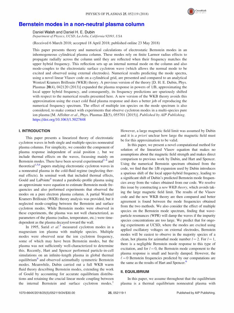
where c � 2xrðX� xrÞ � 1. Densities predicted by Eqs. (1)

and (2) are displayed in Fig. 1 for a set of different c values.

As c approaches zero, the plasma radius (measured in Debye

lengths) increases.

In later work, we will find it useful to define the equilib-

rium radius of the plasma rp as

rp ¼

ffiffiffiffiffiffiffiffiffiffiffiffiffiffiffiffiffiffiffiffiffiffiffiffiffiðrW

0

2rnðrÞ dr

s: (3)

This radius is equal to the radius of an imaginary “top-hat”

plasma whose central density and total particle number (per

unit axial length) are both equal to our plasma. In scaled

units, there is a relationship between c and rp, good when

rp � 1:

rp � 0:513� log cþ 1

2log log 1=c:

Consequently, c parametrizes the scaled radius of the

plasma, i.e., the number of Debye lengths across the column

radius.

The equilibrium distribution function is a product of

n(r) and a rotating Maxwellian, which in our scaled units

becomes

f0ðr; vÞ ¼nðrÞ2p� exp �ðv� xrrhÞ2

2

� �: (4)

For nonneutral plasmas containing multiple species, species

with different masses can centrifugally separate in the rotat-

ing plasma column, with heavier species pushed to the out-

side of the column by centrifugal force effects. According to

the Boltzmann distribution, the ratio of densities between

two species i and j is8

niðrÞ=njðrÞ ¼ ci;j exp ð�ðmi � mjÞx2r r2=2Þ; (5)

FIG. 1. Equilibrium densities scaled by

central density for various values of c.

052119-2 D. Walsh and D. H. E. Dubin Phys. Plasmas 25, 052119 (2018)

where ci;j is a constant depending on the overall concentra-

tion of the two species. Here, however, we will assume that

the density ratio is close enough to a constant over the

plasma profile so that centrifugal separation effects can be

neglected. This is not a good approximation in some very

low temperature experiments (T < 10�4 eV) on ion plasmas

at UCSD, but is a reasonably good approximation at higher

temperatures where, as we will see, it is easier to see

Bernstein modes. Thus, we will assume that each species has

the same radial density profile, multiplied by a factor propor-

tional to the overall concentration of that species.

III. COLD FLUID THEORY OF CYCLOTRON WAVES

In this section, we briefly review the general theory of

cold fluid electrostatic waves in a plasma column. Readers

interested in more details should refer to the original work of

Trivelpiece and Gould,9 as well as a more recent cold fluid

theory of z-independent cyclotron waves developed by

Gould.4,5 Temperature is assumed to be zero in this theory

and the plasma equilibrium density is assumed to have an

arbitrary radial dependence n(r). The theory considers cyclo-

tron waves that are excited by oscillating an external elec-

trode voltage at frequency x. The electrode radius is r¼ rW

and its voltage is oscillated to produce a potential on the

electrode of the form dUWe�ixtþi‘h, where ‘ is an integer. For

a single-species plasma, Gould derived a linear fluid theory

for small amplitude waves, where the perturbed potential

dUðr; h; tÞ is also proportional to e�ixtþi‘h and satisfies the

following boundary-value problem:

r � �rdU ¼ 0; (6)

with a 2-dimensional dielectric tensor � given by

� ¼ 1�1

�iXv

x

iXv

x1þ

rx0f Xv

x2

2666437775Xðx; rÞ: (7)

Here

Xðx; rÞ ¼x2

p

x2 � XvðXv � rx0f Þ; (8)

where we have momentarily relaxed our scaled units, so that

the dependence of X on the plasma frequency xp is apparent

(in our scaled units x2p ¼ nðrÞ). The primes denote deriva-

tives with respect to r, x ¼ x� ‘xf is the Doppler-shifted

wave frequency as seen in a frame rotating with the plasma,

Xv ¼ X� 2xf is the “vortex frequency” (the cyclotron fre-

quency shifted by the Coriolis force from rotation), and

xf ðrÞ is the cold-fluid rotation rate of the plasma (neglecting

the thermal diamagnetic drift correction that affects xr),

which is given by the solution of the quadratic equation

2xf ðX� xf Þ ¼ hnir: (9)

Here, hnir is the average equilibrium density within radius rgiven by

hnir ¼2

r2

ðr

0

�rd�rnð�rÞ: (10)

Equation (6) is merely a restatement of the Maxwell’s

equation r � D ¼ 0, where the electric displacement vector

is D ¼ �� � rdU.

Writing out Eq. (6), one obtains the following second

order differential equation that must be solved for the wave

potential dU:

0 ¼ �11dU00 þ �11

rþ �011

� �dU0 þ i‘

r�012 �

‘2

r2�22

� �dU; (11)

where again primes denote derivatives with respect to r.

Here, �ij refers to the i,jth component of the dielectric tensor.

This equation is to be solved using the boundary conditions

that at r¼ 0 the potential must remain finite, and at the sur-

rounding electrode with radius r¼ rW the potential is

dUðrWÞ ¼ dUW .

Gould made further progress in obtaining the solution of

Eq. (11) by taking a large magnetic field limit in order to

simplify several terms. We will not use this approximation

here because it introduces small but important errors in the

solution. Instead, we solve Eq. (11) numerically. However,

we will later find it useful to compare to the large field solu-

tion, so for completeness we provide the solution below. The

general solution to the large-field ordinary differential equa-

tion (ODE) can be written analytically as a linear combina-

tion of two independent solutions:

dU ¼ Ar�‘ðr

d�r�r ð2‘�1Þ

Dð�rÞ þ Br�‘; (12)

where D(r) is the large-field form for �11,

D ¼ 1�x2

p=ð2XÞx � Xv þ rx0f=2

; (13)

and where the coefficients A and B are determined by the

boundary conditions on the solution.1

For the simplest possible case of a uniform plasma

completely filling the electrode volume out to r¼ rW, Eq. (11)

simply becomes �11r2dU ¼ 0. This implies that either the

potential satisfies Laplace’s equation, so that there is no density

perturbation (and no cyclotron wave) or else �11 ¼ 0, which is

the dispersion relation for upper hybrid waves in the uniform

plasma column. The frequency of these waves (as seen in the

rotating frame) is the upper hybrid frequency, given by

x2 ¼ x2p þ X2

v : (14)

In a uniform plasma, these upper hybrid oscillations can

have any functional form, i.e., r2dU is not determined in

cold fluid theory.

Another case that can be handled analytically is a uni-

form plasma column with radius rp less than rW. In this case,

there are surface waves in addition to the upper hybrid

waves. The surface waves can be excited by the external

electrode potential oscillation, i.e., they are driven to large

amplitude if the external electrode potential oscillates at the

052119-3 D. Walsh and D. H. E. Dubin Phys. Plasmas 25, 052119 (2018)

surface wave frequency. The surface waves themselves have

a potential of the form dU / r‘ inside the plasma and a fre-

quency given by the solution of the equation

‘ð�11 þ i�12Þ ¼ �‘1þ ðrp=rWÞ2‘

1� ðrp=rWÞ2‘: (15)

This equation yields a quadratic equation for the wave fre-

quency whose solution is

x ¼ Xv

26

ffiffiffiffiffiffiffiffiffiffiffiffiffiffiffiffiffiffiffiffiffiffiffiffiffiffiffiffiffiffiffiffiffiX2

4�

x2p

2

rp

rW

� �2‘s

: (16)

The upper sign yields the frequency of the surface cyclotron

wave, while the lower sign yields the frequency of the dioco-

tron wave. When the magnetic field is large, the surface

cyclotron frequency can be approximated as

x ¼ Xv þx2

p

2Xv1� rp

rW

� �2‘" #

: (17)

This surface mode frequency is greater than the vortex fre-

quency but less than the upper hybrid frequency.

Both cyclotron and diocotron waves are incompressible

distortions of the shape of the plasma column that rotate in hwith angular phase velocity given by x=‘, as seen in the

frame of the plasma’s rotation. These surface waves have

finite multipole moments, which is why they can create a

potential outside of the plasma that can be detected on the

wall. For instance, for ‘¼ 1 the plasma center is shifted off-

axis and rotates about the center of the trap at the wave phase

velocity, while for ‘¼ 2 the plasma distorts into a uniform-

density ellipse whose shape rotates about its center.

On the other hand, upper hybrid oscillations in the uni-

form plasma column cannot be detected, or excited, using

wall potentials. For instance, an ‘¼ 0 upper hybrid oscilla-

tion corresponds to any cylindrically symmetric radial veloc-

ity perturbation; such a perturbation will oscillate at the

upper hybrid frequency of the column. This perturbation

obviously conserves total charge, and therefore, by Gauss’

law, creates no field outside the plasma that can be used to

detect or excite the mode.

Similarly, upper hybrid oscillations internal to the

plasma column can be found with any azimuthal mode num-

ber ‘ and (almost) arbitrary radial dependence (again assum-

ing that the plasma column has uniform density). For

instance, any initial ‘¼ 1 density perturbation of the form

dnðrÞeih, chosen so as not to change the center of mass loca-

tion of the plasma (i.e.,Ð rp

0d�r�r2dnð�rÞ ¼ 0), will not create an

‘¼ 1 (dipole) moment and will therefore be unobservable

from outside the plasma. This initial perturbation can then

evolve in two ways, depending on the self-consistent initial

velocity field. That part of the field which is curl-free evolves

as an upper hybrid oscillation; that part which is divergence-

free has zero frequency (as seen in the plasma’s rotating

frame). Although not the subject of this paper, the zero-

frequency modes are “convective cell” vortical motions that

do not change the perturbed plasma density, by construction.

There are an uncountable infinity of such degenerate upper

hybrid oscillations and zero-frequency convective cells, but

only two surface modes (the diocotron and upper-hybrid

branches). Only the surface modes are detectable, or excit-

able, from the wall.

For a nonuniform plasma column with density that

smoothly approaches zero at some radius less than rW, the

surface mode and the continuum of upper hybrid oscillations

now couple in an interesting (and nontrivial) way.

(Something similar can happen with the diocotron surface

mode and the zero-frequency modes.10) As the plasma den-

sity varies, the upper hybrid frequency varies and the spec-

trum of upper hybrid oscillations becomes a continuum that

spans the range from the vortex frequency (where the density

approaches zero) to the central upper hybrid frequency. This

continuum includes the surface plasma frequency, and con-

sequently, the formerly discrete surface plasma eigenmode

becomes a “quasimode”;10 i.e., it is no longer an undamped

eigenmode of the system. However, there remains a damped

plasma response to an external driver that consists of a

phase-mixed potential response from the upper hybrid con-

tinuum, peaked around the former surface plasma frequency.

This is a well-known form of spatial Landau-damping that

has been discussed previously for other types of plasma

waves, such as Langmuir waves11 and Trivelpiece-Gould

modes.12 (Sidenote: ‘ ¼ 0 and ‘¼ 1 are exceptional cases.

For ‘ ¼ 0, there is no surface plasma mode, and there is still

no coupling between an external wall potential and the upper

hybrid continuum (see Sec. VIII D), while for ‘¼ 1 the sur-

face mode remains a discrete “center of mass” eigenmode,

even for a nonuniform column.)

To describe the driven response of a nonuniform plasma

column at frequencies near the cyclotron frequency, one

must now solve Eq. (11) numerically in general (except for

the ‘ ¼ 0 case, which can be calculated analytically, as we

discuss later). However, notice that Eq. (11) has regular sin-

gular points for radii where �11 vanishes, causing dU to

diverge. This occurs when

Xðx; rÞ ¼ 1: (18)

Note that this is the same condition we had when consider-

ing modes in a uniform plasma, resulting in upper-hybrid

oscillations in Eq. (14). Accordingly, we define rUHðxÞ to

be a root of Eq. (18), which we refer to as an upper-hybridradius.

For a single species plasma with a thermal equilibrium

density profile, one can show that there is at most one solu-

tion to Eq. (18), r ¼ rUHðxÞ. However, for multispecies plas-

mas, there can be more than one solution.

To understand the nature of the fluid theory divergences

near an upper-hybrid radius, we perform asymptotic analysis

in Eq. (11) near rUHðxÞ in the case where terms of any order

in 1r are neglected. Dropping all such terms in Eq. (11), we

obtain

dU00 þ �011

�11

dU0 ¼ 0: (19)

052119-4 D. Walsh and D. H. E. Dubin Phys. Plasmas 25, 052119 (2018)

Under typical conditions, the root in Eq. (18) is first-order,

that is, X0ðx; rUHÞ 6¼ 0, so it is viable to expand �11ðrÞ around

rUH. We write

�11 �1

L ðr � rUHÞ; (20)

with L � 1=�011ðrUHÞ, so that Eq. (19) becomes

dU00 þ 1

r � rUH

dU0 ¼ 0: (21)

The order of the equation can be reduced, and the equation

can be directly integrated

dU0ðrÞ ¼ A

r � rUH

: (22)

We should emphasize that Eq. (22) is only correct for r near

rUH and should be regarded as the first term in a series

expansion of dU0 about the point rUH. The next-order terms

in the expansion are proportional to log ðr=rUH � 1Þ, a con-

stant of order unity, and so on.

We would like to integrate this expression to obtain

dUðrÞ. However, the divergence at r ¼ rUH requires careful

consideration of the physics: in any physical plasma there

will be a small effect from particle collisions, causing waves

to damp. Later in the paper, we introduce a simple Krooks

model of collisions. This model has the effect of replacing

the frequency x by xþ i� in Eqs. (6)–(18), where � is the

collision rate. This in turn implies that rUH, the root of the

modified Eq. (18), Xðxþ i�; rÞ ¼ 1, is complex. For small

�, a Taylor expansion of this equation implies that the imagi-

nary part of rUH is

ImðrUHÞ ¼ ��@X=@x@X=@r

����rUH0

¼ � @rUH0

@x¼ � 2x�

x2p@�11=@r

� Dr;

(23)

where rUH0 and Dr are the real and imaginary parts of the

upper hybrid radius, respectively

rUH ¼ rUH0 þ iDr; (24)

and the last form for Dr in Eq. (23) follows by substitution

for X from Eqs. (7), (8), and (18). The sign of Dr can be

either positive or negative depending on the sign of the radial

gradient of �11. The effect of this in integrating Eq. (22) is to

move the pole at rUH slightly away from the real r axis,

allowing integration around the pole

dUðrÞ ¼ A logrUH � r

rUH � r0

� �þ dUðr0Þ; (25)

where r0 is a radius below the cutoff radius, and both rand r0 are close enough to the upper hybrid radius to make

Eq. (20) as good approximation. The coefficient A is given

here by matching to the derivative of the potential using

Eq. (22)

A ¼ �dU0ðr0ÞðrUH � r0Þ: (26)

The logarithmic divergence of the perturbed potential

near the upper hybrid radius can be seen in Fig. 2 for several

different scaled frequencies k,5 where

k ¼ x� XxE

; (27)

and where xE � 1=ð2XÞ is the E�B equilibrium rotation

rate at the center of the plasma column (in our dimensionless

units). (This frequency scaling is useful because the plasma

response to the forcing is largest for frequencies x for which

k is of order unity. The fluid rotation rate xf, given by Eq.

(9), differs from xE at the column center in that it includes

the F�B drift from centrifugal force effects, but this differ-

ence is typically small.) As shown in Fig. 2, the logarithmic

divergence changes with radius as k varies because the upper

hybrid radius is a function of frequency through Eq. (18).

The potential picks up an imaginary part, as shown in

Fig. 2, even for small � because, for r > rUH0, the real part

of the argument of the logarithm in Eq. (25) changes sign

dUðrÞ ¼ A logr � rUH

rUH � r0

� �þ dUðr0Þ þ ipASignðDrÞ: (28)

To determine a resonant surface mode frequency using

these results, we consider a dimensionless measure of the

plasma response Y, the admittance function, defined as

Y ¼rW@dU@r

dU

�����r¼rW

: (29)

Notice that a cylinder containing no plasma is a simple

capacitor, which has purely imaginary experimental admit-

tance (the ratio of current to voltage). Consequently, our the-

oretical definition of Y for a vacant cylinder will be purely

real (the surface charge on the electrode, proportional to

@dU=@rjrW, is the time integral of the current). We conclude

that the imaginary part of Y is due to the presence of plasma,

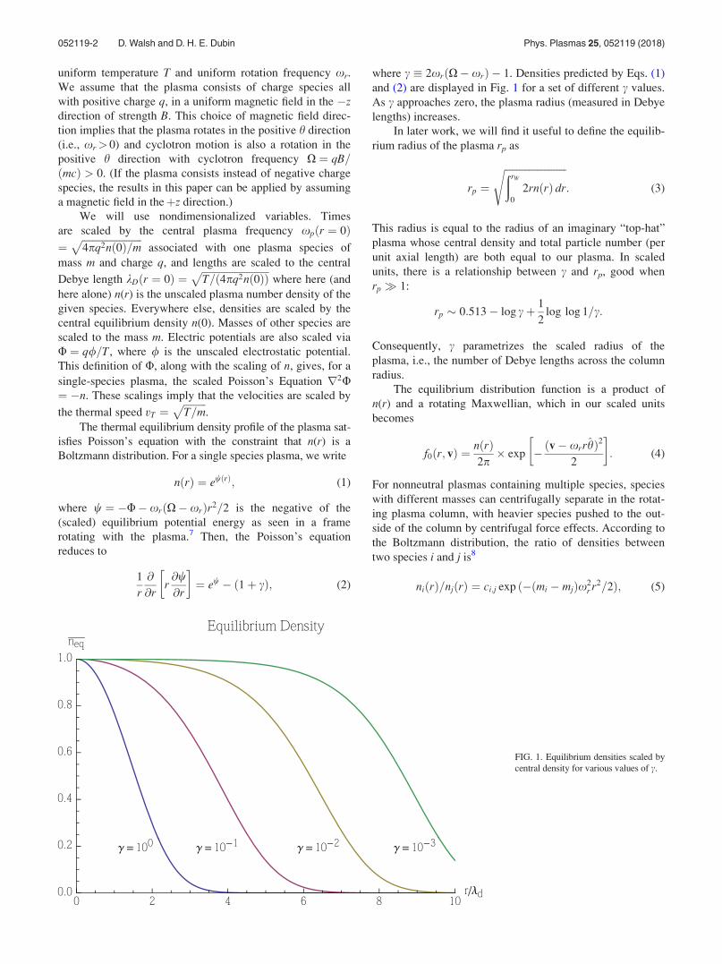
so for the remainder of this paper we will focus on ImðYÞ.For the potential data in Fig. 2, the admittance function is

plotted in Fig. 3. These data show a broad peak, caused by

FIG. 2. Radial dependence of the imaginary part of the perturbed potential

Im dUðrÞ�

driven at frequencies from k¼ 1 (red) down to k ¼ 0:6 (violet)

in equal steps. rp ¼ 4:76, rW¼ 10, ‘¼ 2, X¼ 5, and � ! 0þ.

052119-5 D. Walsh and D. H. E. Dubin Phys. Plasmas 25, 052119 (2018)

the mixing of the continuum of upper hybrid oscillations and

the surface mode, turning the surface mode into a damped

quasimode. The width in this peak decreases as the plasma

edge becomes sharper (i.e., as temperature decreases holding

the plasma radius fixed), approaching a delta function at the

surface cyclotron wave frequency given by Eq. (16) (the

dashed line), when the plasma density approaches a step

function.1

IV. VLASOV SOLUTION

So far, the theory has neglected thermal effects responsi-

ble for Bernstein modes. In this section, we will develop a

numerical approach that keeps these thermal effects. At low

temperatures, the method predicts admittance functions that

approach the cold-fluid theory, but at higher temperatures

Bernstein modes appear as separated peaks in the

admittance.

We will develop a numerical method for solution of the

linearized Vlasov equation in cylindrical coordinates. In

cylindrical coordinates, the Vlasov equation for the distribu-

tion function f ðr; h; vr; vh; tÞ is

@f

@tþ vr

@f

@rþ vh

r

@f

@h� vr

@f

@vhþ vh

@f

@vr

� �þ ð�Xvh þ ErÞ

@f

@vrþ ðXvr þ EhÞ

@f

@vh¼ 0; (30)

with boundary condition at r¼ 0 given by

@f

@h� vr

@f

@vhþ vh

@f

@vr

����r¼0

¼ 0;

and f ! 0 as r !1 and when jvj ! 1. The condition at

r¼ 0 keeps the third term in Eq. (30) from diverging

and physically enforces continuity in f. We will study linear

perturbations away from the thermal equilibrium discussed

in Sec. I. First, we will change velocity coordinates via

v ¼ffiffiffiffiffiffiffiffiffiffiffiffiffiffiv2

r þ v2h

q; tan w ¼ vh

vr, where v is the magnitude of the

velocity, and w is the gyroangle, or the angle of the velocity

relative to the radial direction r . This gives

0 ¼ @f

@tþ v cos w

@f

@rþ v sin w

r

@f

@h� @f

@w

� �þ X

@f

@wþ Er cos wþ Eh sin wð Þ yf

@v

þ �Er sin wþ Eh cos wv

� �@f

@w: (31)

In this form, the boundary conditions simplify to

@f

@h� @f

@w¼ 0; r ¼ 0;

@f

@w¼ 0; v ¼ 0;

f ! 0; r; v!1: (32)

Next, we linearize the equation in the usual way:

f ¼ f0 þ df , where f0 is a time-independent solution to the

non-linear equation. Since the electric potential is deter-

mined by both the external wall potential and the charge den-

sity in the plasma itself, the electric potential is also

expanded as / ¼ U0 þ dU and similarly for the electric

field: E ¼ E0 þ dE. The equilibrium plasma density is azi-

muthally symmetric, so we also use Eh0¼ 0. Self-consistent

magnetic effects are neglected in this treatment, so we omit

the dX term. Here, we will take f0 to be the thermal equilib-

rium solution Eq. (4) solved in Sec. I.

0 ¼ @df

@tþ v cos w

@df

@rþ v sin w

r

@df

@h� @df

@w

� �þ X

@df

@wþ Er0 cos w

@df

@v� sin w

v

@df

@w

� �þ dEr cos wþ dEh sin wð Þ @f0

@v

þ �dEr sin wþ dEh cos wv

� �@f0

@w: (33)

The last term involving a w derivative is cumbersome. To

remove it, we transform into the co-rotating frame with angu-

lar frequency xr. This affects the transformation X! Xv;

Er0! Er0

þ xrðxr � XÞr � Fr0. In these coordinates, @f0

@w

¼ 0 (i.e., where tan w ¼ �vh=vr, with �vh measured in the rotat-

ing frame), eliminating the last term in Eq. (33). Future

appearances of vh will be understood to be measured in the

rotating frame.

We next Fourier analyze in w, h, and t, via

df ðr; h; vr; vh; tÞ ¼ e�ixtþi‘hX1

n¼�1dfnðr; vÞ einw;

dUðr; h; tÞ ¼ dUðrÞe�ixtþi‘h; (34)

where we refer to n as the gyroharmonic number. Finally,

at this point we introduce a Krooks collision term to intro-

duce damping into the system, by adding a term � dfn, driv-

ing the plasma back to equilibrium. This has the effect of

broadening the frequency response, allowing comparison to

experiment and making discrete Bernstein modes visible

numerically. The resulting equation becomes

FIG. 3. A plot of ImðYÞ driven at various frequencies, for the plasma param-

eters of Fig. 2. The colored arrows correspond to the potentials shown in

Fig. 2. The dashed line is discussed in the text.

052119-6 D. Walsh and D. H. E. Dubin Phys. Plasmas 25, 052119 (2018)

ð�ixþ �Þdfn þ Ln;mdfm ¼ ð�ixþ �Þdfn þ L0n;mdfm

þ vf0

�@dU@r

d1n þ d�1

n

2

þ ‘dUr

d1n � d�1

n

2

�¼ 0; (35)

where the second equality gives a definition for the operator

Ln;m and the operator L0m;n is defined as

L0n;mdfm ¼v2

@dfn�1

@rþ @dfnþ1

@r

� �þ v

2r‘þ 1� nð Þdfn�1

� ‘� 1� nð Þdfnþ1

�þ ið‘xr � nXvÞdfn

þFr0

2

�@dfn�1

@vþ @dfnþ1

@v

� ðn� 1Þdfn�1 � ðnþ 1Þdfnþ1

v

�: (36)

Recalling the boundary conditions Eq. (32), and apply-

ing Eq. (34), the boundary conditions become

dfnð0; vÞ ¼ 0; n 6¼ ‘;dfnðr; 0Þ ¼ 0; n 6¼ 0;

dfnðr; vÞ ! 0; r; v!1: (37)

The first and second conditions are unconstrained when n ¼‘ and n¼ 0, respectively. Notice that Eq. (35) does not con-

stitute a closed system for df, since dU also appears. We

close the system by introducing the Poisson’s equation (in

our units), linearizing just as we did above

r2‘dU ¼ �dn; (38)

dn �ð

d2v df ¼ 2pð

dv v dfn¼0; (39)

where the final identity comes from integrating Eq. (34),

where all but the n¼ 0 term drops out.

To drive the plasma with ‘ 6¼ 0 forcing, a forcing poten-

tial on the wall dUWðrW ; h; tÞ ¼ dUWe�ixtþi‘h is introduced

(expressed here with full h and t dependence), which serves

as a boundary condition for the Poisson’s equation, namely,

that dUðrWÞ ¼ dUW . (We discuss ‘ ¼ 0 forcing in Sec.

VIII D.) We facilitate the solution by splitting the perturbed

potential into a sum: dU ¼ dUH þ dUp, where dUH satisfies

the Laplace’s (homogeneous) equation r2‘dUH ¼ 0 subject

to dUHðrWÞ ¼ dUW , with solution dUH ¼ dUWðr=rWÞ‘, and

the plasma potential dUp satisfies the (inhomogeneous)

Poisson’s equation r2‘dUp ¼ �n, with Dirichlet boundary

conditions. By rewriting our equation in terms of dUp; dUH

appears as a source term, so Eq. (35) becomes

½ð�ixþ �Þdn;m þ Lpn;m�dfm

¼ �vf0

@dUH

@r

d1n þ d�1

n

2þ ‘dUH

r

d1n � d�1

n

2

� �; (40)

where Lp specifies that the terms proportional to dU in L of

Eq. (35) are to be replaced with dUp (that is, they solve the

Poisson’s equation with Dirichlet boundary conditions). The

resulting linearized Vlasov equation, along with the

Poisson’s equation and the definition of dn, is

ð�ixþ �Þdn;m þ Lpn;m

h idfm ¼ �

‘ r‘�1v f0 dUW d1n

r‘w;

2pð

dv v dfn¼0 � dn ¼ 0;

r2‘dUp þ dn ¼ 0: (41)

We now regard Eq. (41) as a system of equations for the

functions dfn, dn, dUp, written in some basis. The equations

have been expressed so that the terms linear in the variables

appear on the left-hand side, while sources appear on the

right-hand side. For the numerical work considered here, the

basis chosen is obtained simply by discretizing the phase

space variables r and v. The explicit discretization used will

be discussed in Sec. IV A.

The reader may wonder why dUp appearing in Eq. (35)

wasn’t simply expressed in terms of Green’s functions,

which are themselves functions of dn and therefore df. We

originally approached the problem this way, but when we

began calculating on high-resolution grids we found that the

non-local nature of the Green’s function (in both space and

velocity variables) introduced terms connecting every n¼ 0

grid point to every other, making the resulting matrix equa-

tion extremely dense. While treating df, dn, and dUp may

appear redundant, the sparsity obtained by introducing a

local Poisson’s equation rather than non-local Green’s func-

tion relations far outweighs the marginally increased size of

the matrix equation.

We now show that L0 is anti-Hermitian with respect to

the inner product

ða; bÞ �X1

n¼�1hanjbni; (42)

where

hanjbni �ð1

0

r dr

ð10

v dv anðr; vÞ bnðr; vÞ: (43)

The anti-Hermitian property ensures that, in the absence of

self-consistent effects, normal mode frequencies are purely

real. This is to be expected, since L0 describes a plasma of

test charges moving in a background field, which should

not have modes that grow or decay indefinitely. On the

other hand, if a numerical method was employed that does

not satisfy this anti-Hermitian property, spurious growth or

decay of modes could occur. This possibility will be

addressed when we discuss the discretization of the

equations.

To prove the anti-Hermitian property, we rewrite L0 by

rewriting r and v derivatives using

@fn

@rðr; vÞ ¼ 1ffiffi

rp @

@r

ffiffirp

fnðr; vÞ �

� 1

2rfnðr; vÞ;

@fn

@vðr; vÞ ¼ 1ffiffiffi

vp @

@v

ffiffiffivp

fnðr; vÞ �

� 1

2vfnðr; vÞ;

052119-7 D. Walsh and D. H. E. Dubin Phys. Plasmas 25, 052119 (2018)

which gives

L0n;mfm ¼v

2

1ffiffirp @

@r

ffiffirp

dfn�1 þ dfnþ1ð Þ �

þ ‘þ 1=2� nð Þdfn�1 � ‘� 1=2� nð Þdfnþ1

r

� �þið‘xr � nXvÞdfn þ

Fr0

2

1ffiffiffivp @

@v

ffiffirp

dfn�1 þ dfnþ1ð Þ �

� ðn� 1=2Þdfn�1 � ðnþ 1=2Þdfnþ1

v

� �: (44)

We now form the inner product ðg; L0f Þ. We then apply the

following identities, proved through integration by parts:�gm

���� 1ffiffirp @

@r

ffiffirp

fn

� ¼ �

�1ffiffirp @

@r

ffiffirp

gm

�����fn ; (45)�gm

���� 1ffiffiffivp @

@v

ffiffiffivp

fn

� ¼ �

�1ffiffiffivp @

@v

ffiffiffivp

gm

�����fn

; (46)

�gn

���� ‘� nþ 1

2

� �fn�1 � ‘� n� 1

2

� �fnþ1

¼ �

�‘� nþ 1

2

� �gn�1 � ‘� n� 1

2

� �gnþ1

����fn ; (47)

which demonstrate that all terms appearing in L0 are anti-

Hermitian: ðg; L0f Þ ¼ �ðL0g; f Þ.

A. Numerical grid

The next step is to put Eq. (35) on a grid to be solved

computationally. First, we only keep a finite number of gyro-

harmonics in the solution, jnj < Mw for a given integer Mw

chosen to be sufficiently large to yield convergent results

(more on this later). For n�values beyond this range, we set

dfn ¼ 0. We choose a uniform radial grid with

ri ¼ iDr; i ¼ 0; 1; 2;…;Mr, and a uniform grid in speed vwith vj ¼ jDv; j ¼ 0; 1; 2;…;Mv, writing dfnðri; vjÞ � df n

i;j.

The maximum radius Rmax ¼ MrDr is chosen to be just

outside the plasma, and the maximum speed Vmax ¼ MvDvis chosen to be roughly 4 thermal speeds, i.e., in scaled

units Vmax 4. We discretize the operator using second-

order-accurate centered-differences for the derivatives in rand v.

However, this introduces small, unphysical errors

because the discretized operator L0n;m is no longer anti-

Hermitian. These errors can have the effect of destabilizing

the equations, creating instabilities that result in spurious

grid-scale oscillations in the wave potential and unphysical

peaks in the admittance. This can be ameliorated by carefully

choosing a discretization scheme that preserves the anti-

Hermitian property as much as possible. One such method

rewrites the radial derivatives in Eq. (36) as

@f=@r ¼ ð1=rÞ@ðrf Þ=@r � f=r, and similarly for the v-deriv-

atives, then center-differences these derivatives while aver-

aging some terms over neighboring grid-points in r and v, as

in the Lax method.13 With this modification, the differenced

Eq. (35) becomes

vj

2ri

riþ1ðdf nþ1iþ1;j þ df n�1

iþ1;jÞ � ri�1ðdf nþ1i�1;j þ df n�1

i�1;jÞ2Dr

� n

2ðdf n�1

iþ1;j � df nþ1iþ1;j þ df n�1

i�1;j � df nþ1i�1;jÞ þ ‘ðdf n�1

i;j � df nþ1i;j Þ

� �

þFr0i

2vj

vjþ1ðdf nþ1i;jþ1 þ df n�1

i;jþ1Þ � vj�1ðdf nþ1i;j�1 þ df n�1

i;j�1Þ2Dv

� n

2ðdf n�1

i;jþ1 � df nþ1i;jþ1 þ df n�1

i;j�1 � df nþ1i;j�1Þ

� �

þ vjf0i;j

2

dUiþ1 � dUi�1

2Drðdn;1 þ dn;�1Þ þ

‘dUi

riðdn;1 � dn;�1Þ

� �þ ið‘xr þ nXv � x� i�Þdf n

ij ¼ �‘r‘�1

i vjf0i;jdUWd1n

r‘w: (48)

In both the first and second lines, the two terms proportional

to n are written as the average over their neighboring grid-

points in r and v, respectively, which is correct as the grid

size approaches zero. Using the discretized version of Eq.

(42), where the integrals are replaced with a Simpson’s rule

Riemann sum, this discretized Vlasov equation is also anti-

Hermitian in the absence of the self consistent dUp term,

with respect to the anti-Hermiticity of the continuous equa-

tion. This equation forms a closed linear inhomogeneous sys-

tem of equations when combined with discretized forms of

the density relation and Poisson’s equation shown as

follows:

2pXMv�1

j¼0

1

2ðvjdf 0

i;j þ vjþ1df 0i;jþ1Þ � dni ¼ 0; (49)

dUiþ1 � 2dUi þ dUi�1

Dr2þ dUiþ1 � dUi�1

2riDr� ‘

2

r2i

dUi þ dni ¼ 0;

(50)

along with the boundary conditions from Eq. (37)

df n0;j ¼ 0; n 6¼ ‘; (51)

df ‘0;j ¼ 2f ‘1;j � f ‘2;j; (52)

df ni;0 ¼ 0; n 6¼ 0; (53)

052119-8 D. Walsh and D. H. E. Dubin Phys. Plasmas 25, 052119 (2018)

df 0i;0 ¼ 2f ‘i;1 � f ‘i;2; (54)

df nMr ;j¼ df n

i;Mv¼ 0; (55)

where Eqs. (52) and (54) determine the free gridpoints

through linear interpolation for the special cases at the radial

origin where n ¼ ‘, or at the velocity origin where n¼ 0.

Equations (48)–(50) are used for internal points i ¼ 1;…;Mr � 1; j ¼ 1;…;Mv � 1. The boundary condition on the

discretized perturbed plasma potential dUi is obtained by match-

ing at i¼Mr to a solution to the Laplace equation that vanishes

at the wall: dUMr¼ dUpðRmaxÞ ¼ CðR‘max � ðr2

W=RmaxÞ‘Þ,where the constant C is obtained by matching the derivative,

dU0pðRmaxÞ ¼ C‘ðR‘max þ ðr2W=RmaxÞ‘Þ=Rmax. (The left-hand

side of this equation is discretized in the usual way).

B. Convergence

It is of critical importance to ensure that numerical

results are properly converged; in this problem, numerical

accuracy is improved by increasing the number of grid points

in r and v (namely, Mr and Mv), as well as by increasing the

number of gyroharmonics (namely, Mw) kept in the calcula-

tion. Some exploration is required to discover optimal values

for each of these three numbers, as the results obviously

need to be converged in all three variables simultaneously in

order to have reliable results. When checking for conver-

gence, Mr and Mv were independently incremented by 30 at

a time, and Mw was incremented by two at a time. In this

paper, we report on three ‘ values, ‘ ¼ 0; 2; and 4.

Convergence issues varied in each case.

We found that, in general, Mr and Mv must be increased

as the damping � decreases. This is because we are approxi-

mating the frequency response of our mathematical plasma

with a sufficiently large, discrete matrix equation whose

eigenfrequencies (magnetized van Kampen14 modes) must

do a decent job of covering the frequency range of interest.

As � decreases, the resonance width of these discrete

(numerical) modes will eventually become smaller than their

spacing, at which point the results become unphysical. In

order to probe finer frequency resolution, the number of

eigenvalues must be increased, which is conveniently done

by increasing Mr and Mv. This type of numerical issue typi-

cally manifests itself as an admittance function with

extremely sharp peaks that do not persist as resolution is

increased or move around unpredictably as the grid is

adjusted slightly. The problem is resolved either by increas-

ing � (if less frequency resolution is tolerable), or else by

increasing Mr and Mv.

For the finite damping rates used in the paper, conver-

gence in the admittance results was obtained with a rela-

tively small Mw value compared to the number of r and vgrid points required: Mw � 10 was usually sufficient. For

‘ ¼ 4, the values of Mr and Mv required for convergence

were Mr � Mv � 100. This resolution was sufficient to

resolve the first four to eight admittance peaks, counting

from the right (see Fig. 4); lower frequency peaks beyond

this range correspond to potentials that oscillate more rapidly

in r, requiring higher resolution. Somewhat higher resolution

was also typically required at larger magnetic fields.

For ‘¼ 2, larger values of Mr and Mv had to be used to

resolve just the first few admittance peaks, up to Mr ¼ Mv

¼ 240 and Mw ¼ 10, the maximum values we could run on

the available computers (limited by memory requirements in

the numerical solution of the sparse matrix equation).

We should also mention that there were convergence

issues in the distribution function near r¼ 0 for ‘¼ 2;

namely, rapid unphysical variation in dfn versus r and v, for rwithin a thermal cyclotron radius or so of r¼ 0. The origin

of this rapid variation is unknown, but is clearly an artifact

of the discretization of the linear operator. For ‘ ¼ 4, the

wave potential is small enough near the origin so that this

effect was suppressed, since df is quite small near the origin.

However, in all ‘ values studied this unphysical variation did

not seem to affect the density or potential, which was well-

converged and varied smoothly with radius near r¼ 0.

In test cases we studied, where the solution for

df ðr; h; v;wÞ near r¼ 0 is known analytically for a given per-

turbed potential (as a power series expansion in r), the dis-

cretized Vlasov equation was able to reproduce the

analytical solution for the perturbed density and plasma

potential response, even though the numerical distribution

function was noisy near the origin. As a second check, for

l¼ 2 we added 4th derivative “superdiffusion” terms in r and

v to the discretized Vlasov equation in order to suppress this

grid-scale noise in the distribution function near r¼ 0, and

found that for a scaled superdiffusion coefficient of 10�6 the

solution reproduced the admittance curves without superdif-

fusion, with far less noise in dfn near r¼ 0. These checks

gave us some confidence that the admittance, density, and

potential results were sensible even when the underlying dis-

tribution function was noisy near the origin.

For ‘ ¼ 0, and for the “hot” rp ¼ 4:76 plasma discussed

in relation to Figs. 2 and 3, it was fairly easy to obtain con-

verged admittance results for moderate values of the grid

parameters and moderately strong damping rates, similar to

those used in the ‘ ¼ 4 data. No noise issues near the radial

origin were observed. For a colder plasma we studied, with

rp¼ 43, more radial grid points had to be used in order to

resolve the plasma edge, as one would expect.

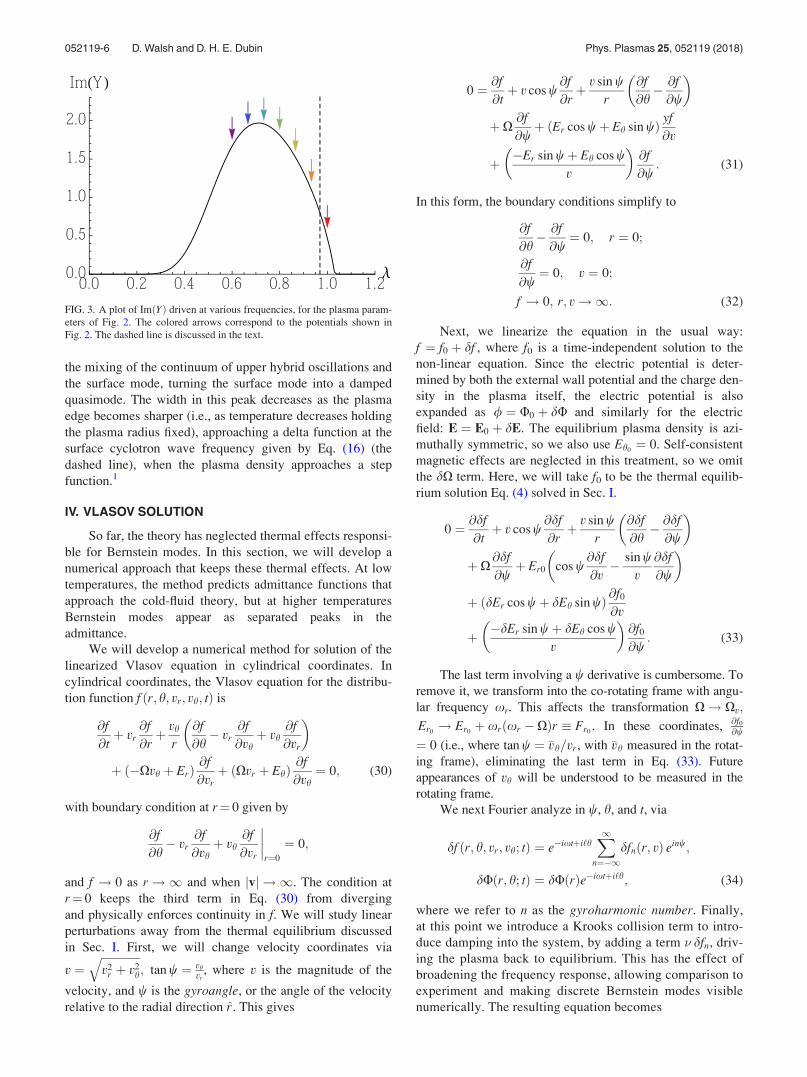
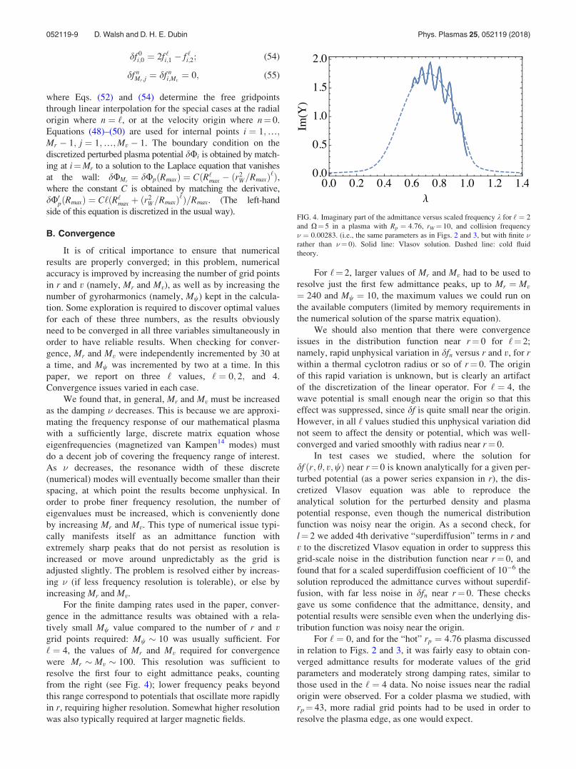
FIG. 4. Imaginary part of the admittance versus scaled frequency k for ‘ ¼ 2

and X¼ 5 in a plasma with Rp ¼ 4:76, rW¼ 10, and collision frequency

� ¼ 0:00283. (i.e., the same parameters as in Figs. 2 and 3, but with finite �rather than �¼ 0). Solid line: Vlasov solution. Dashed line: cold fluid

theory.

052119-9 D. Walsh and D. H. E. Dubin Phys. Plasmas 25, 052119 (2018)

Finally, we encountered a puzzling anomaly that caused

numerical instability for v > vthresh, where vthresh depended

on the radial grid spacing Dr; Mw. When this instability was

present, the perturbed distribution function in phase space

would look normal for small velocities, but for v > vthresh

would appear random. It was discovered that this instability

could be avoided by increasing the quantity DrMw=Vmax,

where Vmax is the highest velocity on the grid, thereby forc-

ing vthresh higher than the highest velocity kept on the grid.

Therefore, we only increase Mr (i.e., decrease Dr) as much

as is needed to resolve the radial variation in the mode, but

no more, unless we are willing to increase Mw.

C. Results

In Fig. 4, we display a characteristic solution taken from

the converged results of the numerical Vlasov code [i.e., the

solutions of (48)–(50)] for the imaginary part of the admit-

tance function versus scaled frequency k [see Eq. (27)]. The

plasma is assumed to have the same parameters as in Figs. 2

and 3, except that in those figures �¼ 0, whereas here we

take � ¼ 0:00283. (As previously mentioned, a finite value

of � is necessary to obtain converged results in the Vlasov

solution.) One can see that the admittance has separated into

a series of peaks whose magnitudes follow the corresponding

cold fluid theory, and whose spacing varies, becoming more

closely spaced as frequency k decreases. Each peak corre-

sponds to a Bernstein mode.

Incidentally, the cold fluid theory admittance plotted in

Fig. 3 differs slightly from the theory presented in Sec. III in

that we took � 6¼ 0 for Fig. 4, just as in the Vlasov theory.

For finite �, the radial dependence of cold fluid theory poten-

tial differs only slightly from that shown in Fig. 2; the sharp

singularity at the upper hybrid cutoff radius rUH0 becomes

slightly rounded.

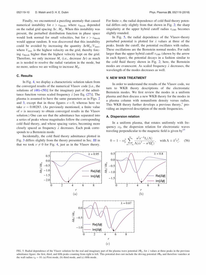
In Fig. 5, the radial dependence of the Vlasov-theory

perturbed potential is plotted for k values at three of the

peaks. Inside the cutoff, the potential oscillates with radius.

These oscillations are the Bernstein normal modes. For radii

larger than the upper hybrid cutoff rUH0 (shown by the arrow

in each figure), the potential decays in a fashion similar to

the cold fluid theory shown in Fig. 2; here, the Bernstein

modes are evanescent. As scaled frequency k decreases, the

wavelength of the modes decreases as well.

V. NEW WKB TREATMENT

In order to understand the results of the Vlasov code, we

turn to WKB theory descriptions of the electrostatic

Bernstein modes. We first review the modes in a uniform

plasma and then discuss a new WKB theory for the modes in

a plasma column with nonuniform density versus radius.

This WKB theory further develops a previous theory,1 pro-

viding an improved description of the mode frequencies.

A. Dispersion relation

In a uniform plasma, that rotates uniformly with fre-

quency xf, the dispersion relation for electrostatic waves

traveling perpendicular to the magnetic field is given by15

0 ¼ 1� x2p

X1n¼�1

n2e�KInðKÞKðx2 � n2X2

vÞ; with K � k2r2

c : (56)

FIG. 5. Radial dependence of the Vlasov solution for the real and imaginary part of the plasma wave potential dUp, for k values at three peaks in the previous

admittance figure: the first, third, and fifth peaks counting from right to left. This potential does not include the driving potential dUH and therefore vanishes at

the wall radius rW¼ 10. (a) First mode, (b) third mode, and (c) fifth mode.

052119-10 D. Walsh and D. H. E. Dubin Phys. Plasmas 25, 052119 (2018)

Here, k is the wavenumber, x is the Doppler-shifted driving

frequency (including Krook collisions) seen in the frame

rotating with the plasma, defined by x ¼ x� ‘xf þ i�, rc is

the thermal cyclotron radius given by rc ¼ 1=Xv in scaled

units, and InðxÞ is a modified Bessel function. To study these

modes near the cyclotron frequency, we ignore all but the

dominant terms in which the denominator is small with

n ¼ 61. With this simplification, the dispersion function

becomes

Dðx; kÞ ¼ 1� 2x2p

e�KI1ðKÞKðx2 � X2

vÞ: (57)

This expression can be related to the fluid theory dispersion

relation involving the function XðxÞ as follows (noting that

X simplifies for a uniform system):

Dðx; kÞ ¼ 1� 2XðxÞ e�KI1ðKÞ

K: (58)

Note that the function 2e�KI1ðKÞ=K is monotonically

decreasing in K with a maximum of unity at K¼ 0. Thus, a

solution to D ¼ 0 requires that XðxÞ > 1, or equivalently

�11 < 0. Thus, propagating Bernstein waves can exist in the

plasma only for frequencies for which �11 < 0. However, if

�11 > 0 there are still solutions to D ¼ 0, but these solutions

require imaginary values of k (i.e., negative K). These are

evanescent (non-propagating) solutions.

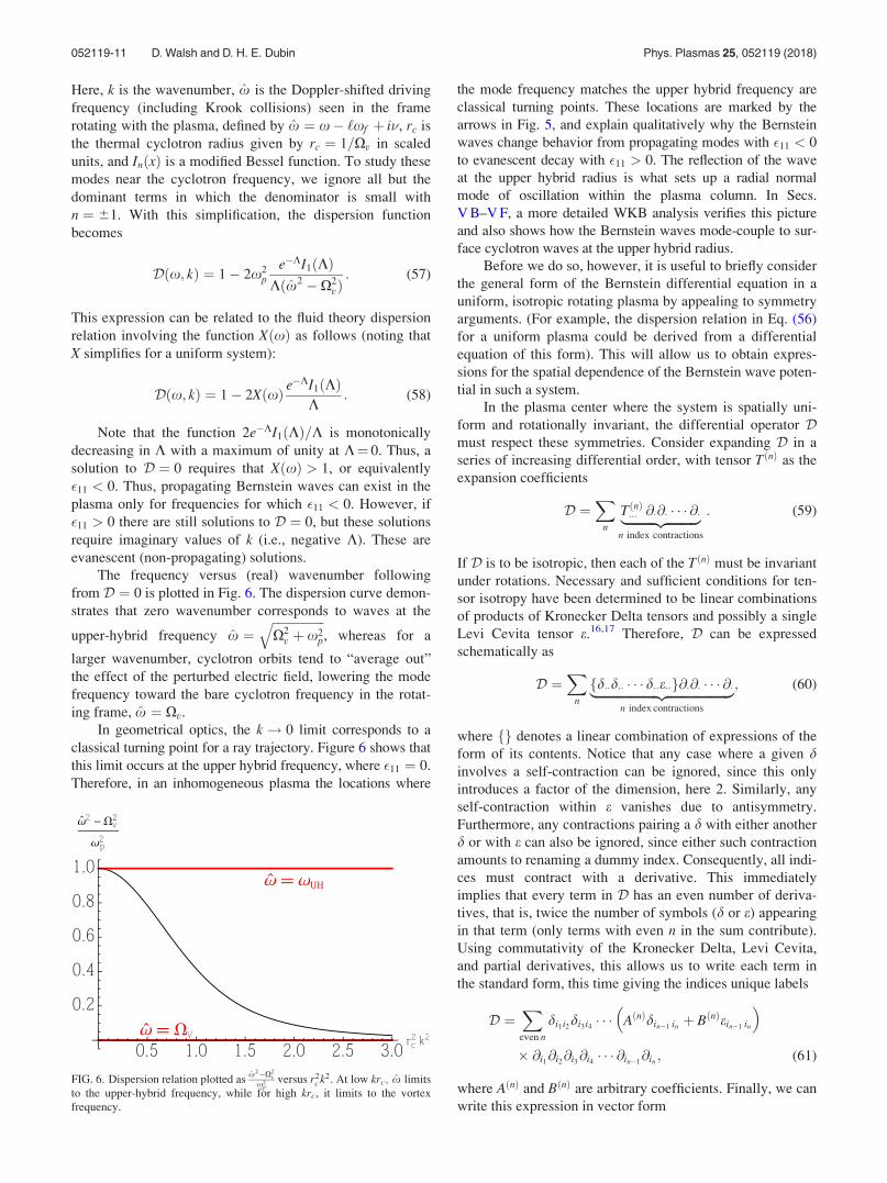
The frequency versus (real) wavenumber following

from D ¼ 0 is plotted in Fig. 6. The dispersion curve demon-

strates that zero wavenumber corresponds to waves at the

upper-hybrid frequency x ¼ffiffiffiffiffiffiffiffiffiffiffiffiffiffiffiffiffiX2

v þ x2p

q, whereas for a

larger wavenumber, cyclotron orbits tend to “average out”

the effect of the perturbed electric field, lowering the mode

frequency toward the bare cyclotron frequency in the rotat-

ing frame, x ¼ Xv.

In geometrical optics, the k! 0 limit corresponds to a

classical turning point for a ray trajectory. Figure 6 shows that

this limit occurs at the upper hybrid frequency, where �11 ¼ 0.

Therefore, in an inhomogeneous plasma the locations where

the mode frequency matches the upper hybrid frequency are

classical turning points. These locations are marked by the

arrows in Fig. 5, and explain qualitatively why the Bernstein

waves change behavior from propagating modes with �11 < 0

to evanescent decay with �11 > 0. The reflection of the wave

at the upper hybrid radius is what sets up a radial normal

mode of oscillation within the plasma column. In Secs.

V B–V F, a more detailed WKB analysis verifies this picture

and also shows how the Bernstein waves mode-couple to sur-

face cyclotron waves at the upper hybrid radius.

Before we do so, however, it is useful to briefly consider

the general form of the Bernstein differential equation in a

uniform, isotropic rotating plasma by appealing to symmetry

arguments. (For example, the dispersion relation in Eq. (56)

for a uniform plasma could be derived from a differential

equation of this form). This will allow us to obtain expres-

sions for the spatial dependence of the Bernstein wave poten-

tial in such a system.

In the plasma center where the system is spatially uni-

form and rotationally invariant, the differential operator Dmust respect these symmetries. Consider expanding D in a

series of increasing differential order, with tensor TðnÞ as the

expansion coefficients

D ¼X

n

TðnÞ��� @�@� � � � @�|fflfflfflfflfflfflfflfflffl{zfflfflfflfflfflfflfflfflffl}n index contractions

: (59)

If D is to be isotropic, then each of the TðnÞ must be invariant

under rotations. Necessary and sufficient conditions for ten-

sor isotropy have been determined to be linear combinations

of products of Kronecker Delta tensors and possibly a single

Levi Cevita tensor e.16,17 Therefore, D can be expressed

schematically as

D ¼X

n

fd��d�� � � � d��e��g@�@� � � � @�|fflfflfflfflfflfflfflfflfflfflfflfflfflfflfflfflfflfflfflffl{zfflfflfflfflfflfflfflfflfflfflfflfflfflfflfflfflfflfflfflffl}n index contractions

; (60)

where fg denotes a linear combination of expressions of the

form of its contents. Notice that any case where a given dinvolves a self-contraction can be ignored, since this only

introduces a factor of the dimension, here 2. Similarly, any

self-contraction within e vanishes due to antisymmetry.

Furthermore, any contractions pairing a d with either another

d or with e can also be ignored, since either such contraction

amounts to renaming a dummy index. Consequently, all indi-

ces must contract with a derivative. This immediately

implies that every term in D has an even number of deriva-

tives, that is, twice the number of symbols (d or e) appearing

in that term (only terms with even n in the sum contribute).

Using commutativity of the Kronecker Delta, Levi Cevita,

and partial derivatives, this allows us to write each term in

the standard form, this time giving the indices unique labels

D ¼X

even n

di1i2di3i4 � � � AðnÞdin�1 in þ BðnÞein�1 in

� �� @i1@i2@i3@i4 � � � @in�1

@in ; (61)

where AðnÞ and BðnÞ are arbitrary coefficients. Finally, we can

write this expression in vector form

FIG. 6. Dispersion relation plotted asx2�X2

vx2

pversus r2

c k2. At low krc; x limits

to the upper-hybrid frequency, while for high krc, it limits to the vortex

frequency.

052119-11 D. Walsh and D. H. E. Dubin Phys. Plasmas 25, 052119 (2018)

D ¼X1i¼0

r2ð Þir � EðiÞ r; (62)

where

EðiÞ ¼ AðiÞ BðiÞ

�BðiÞ AðiÞ

� �:

To match this general form of D to the fluid theory of

Sec. III, we impose the additional constraint that Eð0Þ ¼ �(recall � is the fluid theory dielectric) so that the theories

match to the lowest differential order. Since Bessel

Functions of the first and second kind are always eigenfunc-

tions of r2 and r � EðiÞ r, we can see that CJ‘ðkrÞ þDY‘ðkrÞsatisfies this equation and continuity at r¼ 0 enforces D¼ 0.

Furthermore, since J‘ðkrÞ is locally asymptotic to a plane

wave with wavenumber k far from the origin, k must satisfy

Dðx; kÞ ¼ 0. While this solution is only valid for a uniform

plasma, it also provides an approximate solution to a physi-

cal plasma for r � rp, where n(r) is very nearly constant.

This expression allows us to connect the WKB expression

(valid away from the origin) to this Bessel Function solution

near the center of the plasma.

B. WKB regions

To calculate Bernstein modes in a non-uniform cylindri-

cal plasma, we use a WKB approach. We assume a single-

species plasma for which there is a range of frequencies near

the cyclotron frequency with a single solution to Eq. (18),

i.e., a single upper hybrid radius. In other words, �11

increases monotonically with radius from a negative value

inside the plasma, through zero at the upper hybrid radius,

and increasing toward unity outside the plasma. In this case,

there will be a propagating Bernstein wave for radii less than

rUH0, becoming evanescent for r > rUH0, as in the numerical

results shown in Fig. 5.

In the WKB analysis of these waves, we find that the

perturbed potential can be expressed as a combination of a

fluid theory solution and a radially oscillating Bernstein

wave

dU ¼ dU þ fdU; (63)

where fdU is the radially oscillating Bernstein wave emerging

from finite temperature effects and dU is the non-oscillatory

fluid theory. For radii far from the upper hybrid cutoff, the

fluid theory solution is slowly varying in r and thermal cor-

rections are negligible. We can therefore use cold-fluid the-

ory to describe this solution, numerically integrating Eq. (11)

to obtain dU away from the upper hybrid cutoff. For the

Bernstein solution, on the other hand, we employ the WKB

eikonal approach, matching inner and outer forms for the

eikonals across the upper hybrid radius.

A schematic of the full solution is shown in Fig. 7. We

break the solution into 3 overlapping regions, treated with

different methods, and match the solution across the regions.

In the central region close to r¼ 0, the plasma is nearly uni-

form and we use the Bessel function solution for the

Bernstein wave, derived in Sec. V A. For intermediate radii

between r’0 and the upper hybrid cutoff at r/ rUH, WKB

theory is used. In this region, the Bernstein solution is oscil-

latory. As we pass through the upper hybrid cutoff, the

Bernstein solution transitions from oscillatory to evanescent.

Within this transition region near the cutoff, we solve an

approximate form of the Bernstein differential operator to

match solutions across the cutoff. Here, we find that the

Bernstein solution mode-couples to the fluid solution, mixing

the two in this transition region. A jump condition on

the fluid solution across the transition region is obtained,

describing the effect of this mode coupling on the fluid

solution. A similar jump condition was obtained in Ref. 1,

the difference here being that the fluid solution is treated

exactly (via numerical solution) rather than using an

approximate analytical form valid only for large magnetic

field as in Ref. 1.

C. Central solution

We begin with the solution valid near the center of the

plasma, where the density n(r) is nearly constant for a ther-

mal equilibrium plasma. As we derived previously, the oscil-

latory Bernstein solution for a uniform plasma takes the

form of a Bessel function

fdUðrÞ ¼ Acent J‘ðk0rÞ; (64)

where, for given x, k0 is the solution for k of the Bernstein

dispersion relation, Eq. (58), at the center of the plasma. In

order for this solution to match with the Eikonal solution

FIG. 7. A plot of a typical dU showing the three main regions of the plasma:

dUCENT; dUWKB; dU and dU! referred to in the WKB theory. The region

far outside the plasma is not given a name because it trivially satisfies

Laplace’s equation and has no Bernstein waves.

052119-12 D. Walsh and D. H. E. Dubin Phys. Plasmas 25, 052119 (2018)

described in Sec. V D, we use the large argument expansion

for J‘ðzÞ, giving

fdUcent � Acent

ffiffiffiffiffiffiffiffiffi2

pk0r

rcos k0r � ‘p

2� p

4

� �: (65)

D. Eikonal form

Since a thermal equilibrium plasma does not have a uni-

form density profile n(r), the Bessel function solution intro-

duced in Sec. V C is not satisfactory to describe the entire

interior of the plasma. While the asymptotic central result in

Eq. (65) is a constant wavenumber solution, we now require

k to change as a function of r as the dispersion relation

changes due to the nonuniform plasma density. This moti-

vates a WKB approach to be accurate in the limit where

k� jk0ðrÞ=kj. To the lowest order in WKB theory, the form

of k(r) is found for given x by solving Eq. (58), with X and

Xv the functions of r appropriate for given n(r). This approxi-

mation is only valid away from the cutoff where k ! 0. This

solution is used in the Eikonal in the region that is both far to

the left of the cutoff, and also far from r¼ 0

fdUwkb ¼ AðrÞ cos

ðr

rUH

kð�rÞ d�r þ v

!; (66)

where A(r) is a slowly varying amplitude, the local wave-

number k(r) is found from the Bernstein dispersion relation

Eq. (58) (for given frequency x), and v is a phase factor to

be determined momentarily. The radial form of the ampli-

tude factor is not needed in what follows, but was discussed

in Ref. 1.

Matching the central Eq. (65) and WKB Eq. (66) solu-

tions gives the connection formula that determines the phase

factor v

v ¼ðrUH

0

k dr � ‘p2� p

4: (67)

E. Upper-hybrid cutoff

Near the cutoff, where xUH � x ! 0, the wavenumber

of the WKB solutions also approaches zero (see Fig. 6), so

we can consider adding finite cyclotron radius effects pertur-

batively into Eq. (6)

0 ¼ r � �rdU� r2cr2 ð1� �11Þr2dU

� �: (68)

This approximate expression can be checked by replac-

ing r with ik and comparing the result with Eq. (58),

expanding this dispersion relation to the fourth order in k.

However, it should be noted that this check only verifies the

factor 1� �11, but does not justify its algebraic location

between the two Laplacians. Dubin1 shows, by using integra-

tion over unperturbed orbits in the large magnetic field limit,

why this factor appears in the location it does here. Equation

(68) generalizes the warm fluid theory mode equation of Ref.

1 by not taking the large magnetic field limit. This generali-

zation is important in helping to explain a discrepancy

between the numerical Vlasov solution and the large mag-

netic field WKB analysis of Ref. 1.

We should emphasize that while Eq. (68) is consistent

with the uniform plasma dispersion relation in the small

wavenumber limit, many other forms of the equations could

also be consistent. In fact, Dubin showed that many other

terms appear at Oðr2c Þ in the warm fluid theory equation in

the large magnetic field limit; but he also showed that the

other terms were subdominant in the WKB approximation.

We have no way of knowing what the form of such terms are

when the large magnetic field limit is not taken, so we cannot

prove that such terms are also subdominant to those kept in

Eq. (68). This equation should therefore be regarded skepti-

cally, as an educated guess.

We use Eq. (68) only near the upper hybrid radius and

so we will now approximate its form in this region. Writing

out Eq. (68) in cylindrical coordinates, and multiplying by r2c

to make each term dimensionless, we examine the resulting

terms and drop those terms containing one or more factors ofrc

r , since the upper-hybrid radius is assumed to be many

cyclotron radii from the origin. The result leaves the

following:

�r4c ð1� �11ÞdUð4Þ þ 2r4

c�011dU

ð3Þ þ r2c ð�11 þ r2

c�0011ÞdU00

þ r2c�011dU

0 ¼ 0:

By repeated use of the product rule, this can be partially inte-

grated to obtain

r2c

@

@xð1� �11ÞdU00 �

� �11dU0 ¼ C; (69)

with C a constant of integration (prime represents derivative

with respect to x). To connect with the Eikonal Eq. (66),

which assumes �011=k� 1, we take the dominant balance of

terms, neglecting the term proportional to �011 in the first term

of Eq. (69). Furthermore, we use a linear expansion �11

� ðr � rUHÞ=L near the upper-hybrid cutoff radius, defining

the plasma scale length

L � 1

�@�11

@r; (70)

and write

r2c ð1� �11ÞdU000 �

r � rUH

L dU0 ¼ C: (71)

For r near rUH, the appearance of 1� �11 in the first term can

be replaced with 1, since �11 is small compared to 1 and is

assumed to change gradually anyways. After making this

change, the expression can be manipulated into an inhomoge-

neous Airy equation by the substitution r ¼ rUH þ ðL r2c Þ

1=3 s

dU000 � s dU0 ¼ C0: (72)

The solution to the corresponding homogeneous equation

for dU0 is solved by Airy Functions. We can solve the inho-

mogeneous problem by using variation of parameters to

obtain

052119-13 D. Walsh and D. H. E. Dubin Phys. Plasmas 25, 052119 (2018)

dU0ðsÞ ¼ D1AiðsÞ þ D2BiðsÞ þ D3CiðsÞ; (73)where

CiðsÞ � pAiðsÞðs

�1Bið�sÞ d�s þ pBiðsÞ

ð1s

Aið�sÞ d�s: (74)

The coefficients Di in Eq. (73) are determined by matching

asymptotic forms for the Airy functions to the corresponding

asymptotic forms for the potential to the left and right of the

cutoff. The asymptotic expansions of the Airy Functions are

as follows:

AiðsÞ �

sin2

3ð�sÞ3=2 þ p

4

� �ffiffiffippð�sÞ1=4

; s! �1

exp � 2

3ðsÞ3=2

� �2ffiffiffippðsÞ1=4

; s!1

8>>>>>>>>>><>>>>>>>>>>:

BiðsÞ �

cos2

3ð�sÞ3=2 þ p

4

� �ffiffiffippð�sÞ1=4

; s! �1

exp2

3ðsÞ3=2

� �ffiffiffippðsÞ1=4

; s!1

8>>>>>>>>>><>>>>>>>>>>:

CiðsÞ �1

sþ

ffiffiffipp

cos2

3ð�sÞ3=2 þ p

4

� �ð�sÞ1=4

; s! �1

1

s; s!1:

8>>>>>><>>>>>>:

(75)

From these approximations, we can obtain the solution

for dU by integrating the left-side asymptotic expansion of

Eq. (73) once. While the integral is not an elementary func-

tion, it can nonetheless be carried out in the asymptotic

limit. We can also immediately drop the term containing

BiðsÞ, since the exponential growth outside the plasma is

unphysical. Then, the asymptotic result in the interior of the

plasma is

dU ðsÞ¼D1

�sin2

3ð�sÞ3=2�p

4

� �ffiffiffippð�sÞ3=4

0B@1CA

þD3

�ffiffiffipp

cos2

3ð�sÞ3=2�p

4

� �ð�sÞ3=4

þ logð�sÞ

0B@1CAþD4;

(76)

where the notation dU refers to a solution to the left

of the upper hybrid radius, as in Fig. 6. We can read

off the fluid and Bernstein solutions by separating

oscillatory dependence from the logarithmic diver-

gence. By comparing this expression to Eq. (25), one

can see that the fluid component on the left side of

the upper hybrid radius is

dU ðsÞ ¼ D3 log ð�sÞ þ D4: (77)

To the right of the upper hybrid radius, the asymptotic form

requires that the Airy solution in Eq. (73) be integrated with

the same constant of integration as was obtained in Eq. (76).

To ensure this is the case, use is made of the identitiesÐ1�1 AiðsÞ ds ¼ 1 and limN!1

Ð N�N CiðsÞ ds ¼ 0. Once the

evanescent Bernstein solution dies away, we are left with the

outer fluid solution which now takes the form

dU!ðsÞ ¼ D1 þ D4 þ D3 log ðsÞ: (78)

Note that in Eqs. (77) and (78), s can be replaced by r � rUH

since the multiplicative factor relating r � rUH and s implies

that log ð6sÞ equals log ð6ðr � rUHÞÞ plus an additive con-

stant that can be absorbed into D4

dU ðrÞ ¼ D3 log ðrUH � rÞ þ D4; (79)

dU!ðrÞ ¼ D1 þ D4 þ D3 log ðr � rUHÞ: (80)

These results agree in form with the fluid theory near rUH

from Eqs. (25) and (28). However, the additive constant D1

appears as an amplitude in the oscillatory Bernstein solution.

The Bernstein wave couples to the fluid solution, modifying

it at the radius rUH, and introducing a jump in the form of the

fluid solution across the transition region, due to the

Bernstein wave coupling.

F. Matching solutions across rUH

Evaluating Eqs. (79) and (80) at rUH0, and recalling from

Eq. (24) the definition iDr � rUH � rUH0, we have

dU ðrUH0

Þ ¼ D3 log ðiDrÞ þ D4; dU 0ðrUH0

Þ ¼ �D3=iDr;

dU!ðrUH0

Þ ¼ D3 log ð�iDrÞ þ D1 þ D4;

dU!0ðrUH0

Þ ¼ �D3=iDr: (81)

Note that Dr < 0 according to Eq. (23) because, for the case

of interest here, �11 is a monotonically increasing function of

radius [see the discussion following Eq. (58)].

We can match the oscillatory part of dU to fdUWKB by

comparing Eqs. (66)–(76). To do this, keep in mind that k is

linked with the dielectric through Eq. (58), which as we

approach r ¼ rUH (where �11 is evaluated close enough to the

upper-hybrid radius that it varies linearly in r), becomes

k ¼ffiffiffiffiffiffiffiffiffiffiffiffiffiffiffirUH � r

r2cL

r: (82)

Now use this to determine the integral in Eq. (66)ðr

rUH

kð�rÞ d�r ¼ �2

3rc

ffiffiffiffiLp ðrUH � rÞ3=2 ¼ � 2

3ð�sÞ3=2: (83)

This result can be used to replace the argument of the cosine

and sine functions in Eq. (76) with integrals over k(r),

052119-14 D. Walsh and D. H. E. Dubin Phys. Plasmas 25, 052119 (2018)

allowing us to match this result to the WKB eikonal form of

Eq. (66). Using Eq. (67), the matching requires that

tan v� p4

� �¼ D1

pD3

: (84)

We can then use this expression to solve for D1 and apply

this in Eq. (81) to obtain jump conditions matching the inner

and outer fluid solutions across transition region.

As shown in Fig. 8, we can express log ð�xÞ ¼ log ðxÞ�ip, for all x on the left half of the red line when Dr is nega-

tive. Then, we can use Eq. (81) to relate dU and dU! via

the jump conditions

dU!0ðrUH0

Þ ¼ dU 0ðrUH0

Þ;dU!ðrUH0

Þ ¼ dU ðrUH0

Þ

� iDr p dU 0ðrUH0

Þ tan v� p4

� �þ i

� �:

(85)

For clarity, it should be noted that the choice of rUH0 in

Eq. (85) is merely a convenience. Equation (85) could also

be evaluated at any other point r within the transition region

near rUH, with the substitution iDr ¼ rUH � r. This relies on

the fact that the functional forms of the fluid solutions, Eqs.

(79) and (80), are both valid solutions of the fluid theory

ODE Eq. (25) in the transition region, each matching onto

the numerical fluid solutions on their respective side of the

upper hybrid radius.

In a similar vein, it is informative to consider what is

going on with the jump conditions Eq. (85) as � ! 0. It

appears that the last term in the second condition vanishes as

� ! 0, because Dr is proportional to � [see Eq. (23)].

However, Eq. (81) implies that DrdU 0ðrUH0Þ is independent

of Dr as Dr ! 0, so the last term in the jump condition

remains finite as � ! 0.

These jump conditions provide results for the potential

that are correct to OððDr=LÞ0Þ, neglecting corrections that

are proportional to higher powers of Dr=L. This is because

the conditions rely on low-order asymptotic forms for the

fluid potential in the transition region, Eqs. (79) and (80),

which are correct only up to and including order ðr � rUHÞ0.

As a consequence, the conditions are only useful provided

that Dr=L � 1.

We can now integrate the fluid theory Eq. (6) numeri-

cally from r¼ 0 to rw, using the jump conditions Eq. (85) to

continue integration across the upper-hybrid cutoff. Here, vis evaluated using Eq. (67). This result gives the fluid theory

solution everywhere. Recalling how the perturbed potential

can be expressed as a sum of a fluid theory solution and a

Bernstein wave solution via Eq. (63), and also noting that the

Bernstein wave solution is evanescent outside the upper

hybrid radius, we can calculate the admittance YðxÞ by using

Eq. (29), replacing dU! dU. That is,

Y ¼rW@dU@r

dU

�����r¼rW

: (86)

The value of v in Eq. (85) is obtained using Eq. (67) by inte-

grating over k(r) numerically from r¼ 0 up to r ¼ r0UH,

assuming that � is small so that the difference Dr between

rUH and r0UH can be neglected. For given x, the function k(r)

is obtained by solving the dispersion relation, Eq. (58).

As another check of the jump conditions, in the cold

plasma limit (i.e., as rc ! 0) the argument of the tan func-

tion in Eq. (85) picks up a large negative imaginary part due

to the influence of collisions on k(r), and so

tan ðv� p=4Þ þ i! 0. Then, there is no-longer a jump in

the fluid theory solution across the upper hybrid radius; in

other words, the fluid theory ODE can be integrated without

change from the plasma interior to the wall, resulting in the

same cold fluid admittance function YðxÞ as obtained

previously.

As a final check, we compare the Bernstein mode fre-

quencies obtained from Eq. (85) in the large magnetic field

limit to a result in Ref. 1. In the large-field limit, the fluid

potential for r < rUH0 is given by Eq. (12) with B chosen so

that the solution is finite at r¼ 0:

dU ¼ Ar�‘

ðr

0

dr0r0ð2‘�1Þ

Dðr0Þ ; (87)

where A is an undetermined coefficient. Similarly, using Eq. (12)

to match the outer potential to the potential at the wall yields

dU! ¼ dUWðrW=rÞ‘ þ Cr�‘

ðrW

r

dr0r0ð2‘�1Þ

Dðr0Þ ; (88)

where C is a different undetermined coefficient. Applying

these forms to the jump conditions allows us to determine the

coefficients A and C. The solutions are simplified by keeping

only terms of order Dr0 and noting that DðrUH0Þ �iDr=L.

We find that the first condition implies that A ¼ �CþOðDrÞ and using this in the second condition yields

C

�ðrW

0

dr0r0ð2‘�1Þ

Dðr0Þ þpLr2‘�1UH0 ðtan v�p=4½ �þ iÞ

�¼�dUWr‘W :

(89)

Bernstein modes occur at frequencies for which the coeffi-

cient of C vanishes. This condition can be rewritten as

FIG. 8. Complex plot of x ¼ r � rUH. The real r axis is the red line (noting

that Dr is negative). The dashed green contour relates x to �x while avoiding

the branch cut (blue zig-zag).

052119-15 D. Walsh and D. H. E. Dubin Phys. Plasmas 25, 052119 (2018)

v ¼ p4þ npþ arctan

r1�2‘UH0

pL

��ðrW

0

dr0r0ð2‘�1Þ

Dðr0Þ � ipLr2‘�1UH0

�;

(90)

where n is any integer and the main branch of the arctan

function is taken. Using Eq. (67) and noting that, for small

Dr=L, the Plemelj formula can be applied to integrate past

the pole in the integral over 1=Dðr0Þ, we obtainðrUH0

0

kdr ¼ ð‘þ 1Þp2

þ np� arctan

�r1�2‘

UH0

pL PðrW

0

d�r�rð2‘�1Þ

Dð�rÞ

�;

(91)

where P indicates that the principal part of the integral is

taken. This expression for the Bernstein mode dispersion

relation in the large field limit agrees with Eq. (152) in Ref.

1 (with a redefinition of the integer n to n � 1).

VI. VLASOV vs. NEW WKB AND OLD WKB THEORIES

We now present the results of the new WKB theory for

various magnetic fields, values of ‘, and density profiles,

comparing the theory to numerical solutions of the Vlasov

equation and to the prior large magnetic field WKB theory.1

We first study a ‘ ¼ 4 perturbation in a plasma with

rp ¼ 4:76; rW ¼ 10;X ¼ 5, and � ¼ 1=300. These parame-

ters are similar to a case studied by Dubin. In Fig. 9, we

compare the new WKB solution for the admittance to the

Vlasov numerical method and to the prior WKB theory.1

The new WKB theory produces a mode frequency pre-

diction that is closer to the Vlasov solution than the old

WKB theory. Again, the shift in the frequency between the

old and new theories arises from the large magnetic field

approximation for the cold-fluid dielectric that was used in

the old theory. Also, both WKB theories have a slight, but

consistent overestimation of the admittance. This is probably

related to finite temperature corrections to the cold fluid the-

ory that are neglected in the WKB approach used here.

In the next figures, we vary the magnetic field strength.

In Fig. 10, we vary X from 4 to 10 for an ‘ ¼ 4 perturbation,

and in Fig. 11, we do the same for an ‘¼ 2 perturbation. For

a given peak (corresponding to the number of radial nodes in

the wave), the relative error in the scaled mode frequency ktends to decrease as magnetic field increases from X¼ 4 to

X¼ 10. (This is easiest to see in the second and third peaks,

counting from the right). This is because the criterion for

WKB theory to be valid is k0ðrÞ=k� k and k increases as

magnetic field increases. This WKB criterion can also be

written as kL � 1 since k=k0 L.

Interestingly, for a given magnetic field strength the fig-

ures show that the WKB method tends to produce more

accurate results toward the right side of the plots, for larger

frequencies and therefore smaller k (although the WKB the-

ory tends to predict a weak extra peak at the largest frequen-

cies and for smaller magnetic fields). This can be understood

because k0=k also varies as the frequency varies. As the fre-

quency drops, k0=k becomes larger because the upper hybrid

radius shifts to a larger radius where the density profile is

steeper. A second reason for the increase in k0=k at lower fre-

quencies is the appearance of wave-particle resonances.

These resonances occur at radii rwpr where the dielectric con-

stant �11 diverges. According to Eq. (7), the divergences

occurs where x2 � XvðXv � rx0f Þ ¼ 0. Around such loca-

tions there is a strong resonant interaction between the wave

electric field and particle cyclotron motion, which causes

Landau damping of the wave. WKB theory breaks down

here because as �11 diverges k0 also diverges. In Fig. 12, we

plot the WKB criterion k0Lmin versus frequency, where

Lmin ¼ min½Reð�11=�011ðrÞÞ� is the minimum gradient scale

length across the radial profile and k0 ¼ Re½kðr ¼ 0Þ� is the

FIG. 10. A family of Admittance plots (solid: Vlasov theory; dashed: New

WKB theory). rp ¼ 4:76, rW¼ 10, and ‘ ¼ 4. 1=� ¼ 2000� 2X�10

2 (traces

shifted vertically in steps of 1/20, with X¼ 10 trace unshifted).

FIG. 9. Comparison of Vlasov and WKB approximations, for X¼ 5,

rp ¼ 4:76, rW¼ 10, ‘ ¼ 4, and � ¼ 1=300. Vlasov code uses Mw¼8,

Mr ¼ Mv ¼ 120.

FIG. 11. A family of Admittance plots (solid: Vlasov theory; dashed: New

WKB theory). rp ¼ 4:76, rW¼ 10, and ‘¼ 2. 1=� ¼ 2000� 2X�10

2 (traces

shifted vertically in steps of 1, with X¼ 10 trace unshifted).

052119-16 D. Walsh and D. H. E. Dubin Phys. Plasmas 25, 052119 (2018)

real part of the central wavenumber. The WKB convergence

parameter k0Lmin approaches zero at the first appearance of a

wave-particle resonance in the plasma, which occurs at fre-

quencies on the left side of the plots for ‘¼ 2 and ‘ ¼ 4. The

WKB parameter also decreases at higher frequencies, to the

right side of the plots where the wavenumber of the modes is

smaller. Consequently, the WKB method should work best

at intermediate values of the frequency (and, of course, at

larger magnetic fields). This expected behavior roughly cor-

responds to the results shown in Figs. 9–11.

VII. LIMITING FORM FOR THE MODE FREQUENCIES

It would be useful to have an analytical expression to

approximate the Bernstein Mode frequencies without having

to numerically solve the fluid theory solution and impose a

jump condition at rUH. In this regard, the analytical large

magnetic field dispersion relation used in the old WKB the-

ory, Eq. (91), is useful. A significant simplification can be

made in the limit where the wall radius is large, rw=rp !1.

In this case, the argument of the arctan function in Eq. (91)

approaches infinity. For instance, in the former limit, the

Cauchy Principal integral is dominated by the vacuum region

where D ! 1, and the integrand grows without bound as a

simple power law. Consequently, the argument of the arctan

term approaches p=2. Making this approximation, Eq. (91)

can be simplified to readðrUH

0

kdr ¼ ‘

2þ n

� �p: (92)

Although this result was obtained from the large magnetic

field limit of the theory, it no-longer depends on the large-

field fluid solution and so we might hope that it is more gen-

erally correct. We will test this hypothesis below. First, how-

ever, to standardize the integer n so that n indexes the modes

starting from 1, we impose the constraint that the integral in

Eq. (92) must be strictly positive, since k> 0 for

0 < r < rUH. The issue is that ‘=2 term can be larger than 1,

meaning that subtracting 1 from n¼ 1 (the lowest solution,

by definition) would still produce a strictly positive right-

hand side solution, which is not what we want. To solve this,

we redefine n to absorb the largest integer that is still strictly

less than ‘=2. The effect is that the right-hand side reads npwhen ‘ is even, and ðn� 1=2Þp when ‘ is oddðrUH

0

kdr ¼ ðnþmodð‘; 2Þ=2Þp: (93)

Again, Eq. (93) assumes that rw=rp is large. The func-

tions k(r) and rUH must be calculated exactly using Eq. (57)

as a function of the driving frequency. This result is similar

to a result in Ref. 1, where instead the limit L=rUH � 1 was

assumed; i.e., a nearly square density profile. While we tried

assuming a square profile with upper hybrid radius equal to

the plasma radius by writingÐ rUH

0kdr kð0Þrp, this

completely misrepresents the lowest-order modes because

rUH actually increases from zero quite rapidly for the first

few modes due to the non-rectangular profile. Unfortunately,

correct determination of Bernstein mode frequencies is

strongly dependent on the assumed plasma profile. To under-

stand this strong dependence, we can think of the right-hand

side of Eq. (93) (divided by p) as counting the number of

half-wavelengths within a radius rUH. For the low-order

modes, rUH is very sensitive to the profile shape in the nearly

uniform region of the plasma [since even a small variation in

the falloff of k(r) corresponds to a large variation of rUH due

to the small gradient of k(r)]. Consequently, even if k(r)

were known precisely, the number of half-wavelengths

within this variable rUH is also variable. On the other hand,

for higher order modes, while rUH is less sensitive to the pro-

file shape (since rUH falls somewhere in the relatively thin

plasma edge), k(r) is larger, so even a small variation in rUH

admits a larger variation in the number of allowable half-

wavelengths. In Fig. 13, the new WKB theory peaks are

plotted against the prediction of the mode frequencies for an

infinite wall radius via Eq. (93). As can be seen, the mode

frequencies are very well predicted by Eq. (93) for the infi-

nite wall radius, even for a warm plasma that doesn’t satisfy

rUH � L.

FIG. 13. Determination of mode frequencies from Eq. (93). Orange curve:Ð rUH

0k dr, horizontal lines: ðnþmodð‘; 2Þ=2Þp, vertical lines: intersection of

orange curve with horizontal blue lines, red peaks: ImY from the new WKB

theory multiplied by ðrW=rpÞ2‘ (scaled vertically to fit). X¼ 10,

Rp ¼ 20; ‘ ¼ 2; rw=rp ¼ 1.

FIG. 12. The WKB parameter k0Lmin plotted versus scaled frequency k for a

range of magnetic fields and for both ‘¼ 2 (left) and ‘ ¼ 4 (right), for the

waves and magnetic fields considered in Figs. 10 and 11. WKB theory works

best when k0Lmin � 1.

052119-17 D. Walsh and D. H. E. Dubin Phys. Plasmas 25, 052119 (2018)

VIII. EXTENSION TO MULTIPLE SPECIES

The analysis of Secs. IV and V can be extended to a

multi-species plasma in a straightforward way. We make the

assumption that the plasma is warm enough to not be centrif-

ugally separated, which is done both as a simplifying

assumption for the theory and for comparing to experiments

that operate in this regime, where Bernstein modes are more

easily observed.

A. Resonant species approximation with no speciesseparation

If the plasma species are not centrifugally separated, the

densities of each species are related according to

naðrÞ ¼ dantotðrÞ; a ¼ 1; 2;…n;

where da ¼ nað0Þ=ntotð0Þ is the central species concentration

of species a. Consequently, knowledge of ntot, along with the

species fractions, is sufficient to determine the equilibrium

for each species individually. To calculate this equilibrium,

we note that under the approximation that the species are not

centrifugally separated, the total unperturbed density ntot

behaves as a single species, so the equilibrium Eq. (2) still

holds, where all quantities are normalized to the central

parameters associated with the total plasma.

Then, the multi-species generalization of the local WKB

dispersion function Eq. (58) is

Dðx; k; rÞ ¼ 1� 2X

a

Xaðx; rÞe�Ka I1ðKaÞ

Ka; (94)

where Ka ¼ k2r2ca and Xa can be written as

Xaðx; rÞ ¼x2

pa

x2 � XvaðXva � rx0f Þ: (95)

Here, Xva ¼ Xa � 2xf , and Xa; xpa, and rca are the cyclo-

tron frequency, plasma frequency, and cyclotron radius of

species a, respectively. As in Eq. (58), we have dropped res-

onant terms at multiples of the cyclotron frequency for each

species, since we are interested in the main resonance at the

fundamental cyclotron frequency. There will then be a solu-

tion of the dispersion relation D ¼ 0 for each species; i.e.,

each species has a cyclotron wave associated with it.

In order to make further progress, we will simplify this

result assuming that the magnetic field is large. In this case,

we know that the plasma response is peaked in a narrow fre-

quency range around the cyclotron frequency for each spe-

cies, with x� Xa x2pa=Xa. We assume that the magnetic

field is large enough so that this range is small compared to

the difference between any two cyclotron frequencies:

Xa � Xb � x2p=X. In this case, for cyclotron waves associ-

ated with a given species b with x Xb, only the resonant

term with a ¼ b needs to be kept in the sum in Eq. (94)

because Xa � Xb, and the equation simplifies to

Dðx; kÞ ¼ 1� 2XbðxÞe�KbI1ðKbÞ

Kb: (96)

In other words, in this approximation we ignore the

response of all non-resonant species. In this case, the WKB

theory carries through just as for a single species (the reso-

nant species). Also, this approximation can easily be applied

to the numerical Vlasov solution. Here, all species contribute

to the equilibrium electric field appearing in Eq. (33), but dfis evaluated only for the resonant species.

B. Necessary conditions for Bernstein modes

An important question to consider is “Under what condi-

tions are Bernstein modes possible in a multi-species thermal

equilibrium plasma?”. As previously discussed for a single-

species plasma, Bernstein waves can only propagate when

Reð�11Þ < 0. For a multi-species plasma in the resonant spe-

cies approximation, this corresponds to Xb > 1 for resonant

species b. There is a range of frequencies near Xb where this

inequality is satisfied. To find this range, we utilize the high

magnetic field limiting form of Xb

Xb ¼db � n

kþ ð2� ‘Þhni þ rhni0

2

¼ db � nkþ ð1� ‘Þhni þ n

; (97)

where n is the total density scaled to the total density at

r¼ 0, k � x�Xb

xE; xE ¼ 2pecnðr ¼ 0Þ=B is the central E � B

rotation rate, hni is the average total density within a radius

r, and db is the fraction of the mode resonant species b. The

final expression follows by carrying out the radial derivative

of hni. The expression in Eq. (97) is useful because it allows

insight into where both the cutoffs and wave-particle reso-

nances occur

k ¼ ð‘� 1Þhnir � ð1� dbÞ nðrÞ cutoffð Þ; (98)

k ¼ ð‘� 1Þhnir � nðrÞ resonanceð Þ: (99)

At the cutoff, Re½Xb� ¼ 1 (Re½�11� ¼ 0) while at the wave-

particle-resonance, Xb !1. A cutoff is typically required

in order for propagating solutions to exist because �11 ¼ 1

outside the plasma but Re½�11� < 0 is necessary for wave

propagation. Another way for �11 to change sign is to go

through infinity, at a wave-particle-resonance (WPR).

However, a wave-particle resonance in the plasma strongly

Landau-damps the Bernstein waves, so we look for condi-

tions where the plasma has a cutoff but no resonance. For

‘¼ 0 or ‘¼ 1, Eqs. (98) and (99) imply that a cutoff is

always accompanied by a resonance at a somewhat larger

radius, so the Bernstein response is heavily damped.

However, for ‘ > 1 one can find a frequency range with a

cutoff but no resonance. The right-hand sides of Eqs. (98)

and (99) are functions of r and have maximum values as a

function of r. Note that the maximum value for the wave par-

ticle resonance condition is clearly less than that for the cut-

off condition.

Thus, for Bernstein modes to occur, k must be less than

the maximum value given by Eq. (98) but greater than the

maximum given by Eq. (99): kwpr < k < kcut where

052119-18 D. Walsh and D. H. E. Dubin Phys. Plasmas 25, 052119 (2018)

kcut ¼ max ð‘� 1Þhnir � ð1� dbÞ nðrÞ� �

; (100)

kwpr ¼ max ð‘� 1Þhnir � nðrÞ� �

; (101)

and where maxðÞ is the global maximum operator as r varies.

Notice that the wave-particle resonance does not depend on

db because db does not appear in the denominator of Xb. In

fact,

kwpr ¼ kcutjdb!0: (102)

Consequently, plasmas with a small fraction db of the reso-

nant species exhibit Bernstein modes only over a narrow

range of frequencies, so future experiments on Bernstein

modes should strive to make the resonant species fraction as

large as possible.

The next task is to understand the dependence of kcut

and kwpr on the remaining parameters of the plasma, db, rp,

and ‘. In Fig. 14, it is clear that the Bernstein range in k satis-

fies ‘� 2 < k < ‘� 1, with warmer (i.e., smaller rp) plas-

mas extending through that entire range, except for ‘¼ 2,

which first acquires a wave-particle resonance at a higher

frequency than k ¼ ‘� 2 ¼ 0. It is also interesting to note

that in the case of ‘ ¼ 4, the bottom limit of xwpr becomes

constant at sufficiently small rp due to the appearance of a

second wave-particle resonance that first appears at the very

center of the plasma, at a higher frequency than the wave-

particle resonance appearing at non-zero r. The kinks in the

curves for kcut at various db show whether the region in

which there are Bernstein wave solutions is a disk-shaped

region or an annular region. That is, for sufficiently large rp,

the plasma has two upper hybrid radii. These annular solu-

tions only occur for db < 1.

To understand the fluid theory in a concrete situation,

we now study a particular plasma with parameters chosen to

match some typical experimental conditions. Figure 15

shows several traces of �11ðrÞ ¼ 1� Xb for a range of driv-

ing frequencies. The red (dotted) curve shows the lowest

frequency for which some part of the plasma has �11 < 0 for

�¼ 0, due to the dip in �11 at roughly r¼ 11.5. This fre-

quency is how we defined kcut, as shown by the dashed lines

in Fig. 14. In this case, �11 < 0 only in a small region away

from the origin, that is, this plasma exhibits Bernstein modes

in an annular region, with evanescence both near the plasma

center, and at the very edge of the plasma. As the driving fre-

quency is lowered further, the dip in �11 becomes increas-

ingly deep until at some frequency kwpr the denominator

appearing in �11 vanishes and two wave-particle resonances

are produced that damp out the Bernstein waves, as indicated

by the thick black lines in Fig. 14.

C. Multi-species results

In Fig. 16, we compare the multi-species results of the

WKB theory for ‘¼ 2 modes in an X¼ 10, rp ¼ 4:76

plasma, with two values of the resonant species purities db,

using the resonant-species approximation discussed previ-

ously. First, we take db ¼ 80%. Notice that the right side of

Fig. 16 is at k ¼ 0:8, in agreement with the prediction by

Fig. 14, since no Bernstein peaks appear at frequencies

FIG. 15. �11ðrÞ in a plasma with ‘¼ 2, X¼ 10.45, rp¼ 10.5, db¼ 56.3%, rw

¼ 83.54, with driving frequencies starting from k ¼ 0:711 (red, dotted),

down to k ¼ 0:568 (blue, solid). Locations where �11ðrÞ ¼ �011ðrÞ ¼ 0

labeled.

FIG. 16. Imaginary part of the admittance for a multi-species plasma, using

the WKB theory, for two resonant species fractions, db ¼ 60% and 80%.

X¼ 10, rp¼ 4.76, rW¼ 10, ‘¼ 2 and 1=� ¼ 4000. Compare the fall-off of

the response to the predictions for kwpr and kcut provided by Fig. 14

(arrows).

FIG. 14. Predicted ranges of k over which Bernstein modes occur in WKB

theory for a multispecies plasma without species separation: kwpr < k< kcut, as a function of scaled plasma radius for ‘¼ 2 through ‘ ¼ 4, with

resonant species fraction db 2 f100%; 80%; 60%; 40%; 20%g. Here, kcut is

shown as dashed curves for the different species fractions, and kwpr is shown

as the thick solid lines. The plasma response for ‘ � 1 does not exhibit

Bernstein modes in WKB theory.

052119-19 D. Walsh and D. H. E. Dubin Phys. Plasmas 25, 052119 (2018)

higher than this according to WKB theory. There appears to

be a significant reduction in peak spacing compared to the

pure plasma case (Fig. 11).

Next we consider an identical plasma except with

db ¼ 60%. Again, the plot starts on the left at k ¼ 0:6, as

expected from the appearance there of an ‘¼ 2 wave-particle

resonance in this profile shown in Fig. 14. We also observe

that the Bernstein peaks are more difficult to observe in a

db ¼ 60% plasma, especially for frequencies approaching

kcut than it was for the db ¼ 80% plasma. This is because the

peak spacing is even closer together in the db ¼ 60%

plasma.

D. ‘50 Bernstein modes

We now briefly consider excitation and measurement of

the ‘ ¼ 0 plasma response to an external perturbation near

the cyclotron frequency and compare these results to simula-

tions by Hart and Spencer of ‘¼ 0 cyclotron waves.6 There

are two ways in which the ‘¼ 0 plasma response differs

from the ‘ 6¼ 0 response discussed previously.

First, for ‘ ¼ 0 a wave-particle resonance occurs that

strongly damps Bernstein modes. Although previously we

argued that Bernstein waves are completely absorbed at a

wave-particle resonance, we will see that sometimes a weak

Bernstein mode can still be set up. When the resonant radius

occurs in the region of the plasma edge, and if this edge den-

sity falls rapidly to zero, a new effect occurs: Bernstein

waves are partially reflected at the sharp plasma boundary

rather than being completely absorbed, creating a damped

standing wave inside the plasma. This is an effect beyond

WKB theory. We therefore rely on numerical Vlasov solu-

tions, comparing them to the predictions of cold fluid theory

(which does not include the Bernstein response at all), and to

the particle simulations of Hart and Spencer.

Second, we cannot drive an ‘¼ 0 plasma wave using

an external wall potential, since a cylindrically symmetric

z� independent wall potential does not create a radial elec-

tric field for r < rW . Also, ‘¼ 0 plasma oscillations cannot

be detected at the wall, by Gauss’s law in two-dimensions.

(Experimentally, there can be z-dependence in the driver,

and the plasma is finite-length, but such effects are beyond

the two-dimensional theory presented here). We therefore

must drive the plasma in a different manner than for ‘ 6¼ 0

and we must diagnose the modes using a new definition of

plasma admittance.

We will drive the plasma with an oscillatory h-indepen-

dent potential of the form dUextðrÞe�ixt, where dUextðrÞ does

not satisfy the 2-D Laplace equation; instead we simply take

dUextðrÞ ¼ Ar2. One can think of this as some approximation

to the effective 2-D (z-averaged) driving one would obtain in

a finite-length plasma from a z-dependent wall voltage.

Next, we require a new form for the admittance func-

tion. Hart and Spencer define their measure of the ‘¼ 0

plasma response as the amplitude of the radial component of

the fluid velocity, dVr, at a fixed location on the interior of

the plasma, rmeas. We will use a related dimensionless quan-

tity we call Ya, the “acceleration admittance,” defined as the

(negative of) the radial acceleration of a fluid element at a

given location rmeas, divided by the acceleration produced by

the external potential only

Ya � �ixdVr

@dUext=@r

����r¼rmeas

: (103)

Like the admittance Y, the quantity Ya is independent of

the amplitude A of the external driving potential; its imagi-

nary part depends only on the plasma response; and it is

sharply peaked at the frequencies of weakly damped normal

modes.

There are (at least!) two ways to determine this admit-

tance function from the Vlasov solution. In one method, one

can integrate the numerically determined distribution func-

tion df over velocities to determine dVr and use this result in

Eq. (103). Another, simpler method uses a relation between

dVr and the perturbed plasma potential, dUp. To derive this

relation, begin with the linearized continuity equation

�ixdnþr � ndVþ dnVf

� �¼ 0; (104)

where Vf ðrÞ ¼ xf ðrÞrh is the equilibrium cold-fluid rota-

tional velocity and n(r) is the equilibrium density [see Eqs.

(1) and (9)]. Integrating this equation over a disk of radius rcentered with the plasma and using the divergence theorem,

we obtainþndV � ndsþ

þdnVf � nds ¼

ðixdnd2r: (105)

The second term on the left vanishes due to the purely azi-

muthal equilibrium flow. Using the Poisson equation

r2dUp ¼ �dn; (106)

another application of the divergence theorem, and cylindri-

cal symmetry for ‘¼ 0, the right side of Eq. (105) can be

expressed in terms of the radial plasma electric field, which

gives the following expression for the perturbed radial veloc-

ity for an ‘¼ 0 plasma:

dVrðrÞ ¼ �ix

nðrÞ@dUp

@r: (107)

We will use this result in Eq. (103) to determine the

plasma response to an external potential oscillation for ‘¼ 0

using the Vlasov code. We will also compare these numeri-

cal Vlasov code results to the predictions of cold fluid the-

ory. However, since the driving potential does not satisfy the

Laplace equation, the cold fluid theory of Eq. (6) must be

modified. The linearized cold fluid equations from which it

is derived are the continuity and Poisson equations Eqs.

(104) and (106), as well as the linearized momentum

equation,

�ixdVþ Vf � rdVþ dV � rVf

¼ �rdUp �rdUext � XdV� z: (108)

These three equations can be combined to yield

r � � � rdUp ¼ r � ð1� �Þ � rdUext; (109)

052119-20 D. Walsh and D. H. E. Dubin Phys. Plasmas 25, 052119 (2018)

where � is the cold-fluid dielectric tensor given by Eq. (7).

This is a generalization of Eq. (6) to forcing potentials that

do not satisfy the 2-d Laplace equation. If dUext did satisfy

the Laplace equation, it could be combined with the plasma

potential dUp as dU ¼ dUp þ dUext and dU would satisfy

Eq. (6).

For ‘¼ 0 Eq. (109) can be solved analytically. Writing

out the gradients in cylindrical geometry yields

1

r

@

@rr�11

@dUp

@r

� �¼ 1

r

@

@rrð1� �11Þ

@dUext

@r

� �: (110)

This equation can be integrated once. The constant of inte-

gration must be dropped to keep the potential finite at the ori-

gin, and therefore, we have

@dUp

@r¼ 1� �11

�11

@dUext

@r: (111)

Applying this expression to Eq. (107) and using this result in

Eq. (103) yield the following expression for the acceleration

admittance in cold fluid theory:

Ya ¼x2ð�11 � 1Þ

nðrÞ�11

����r¼rmeas

: (112)

In Fig. 17, we compare the cold-fluid prediction for

Im½Ya� from Eq. (112) to the numerically determined val-

ues from the Vlasov code for the standard plasma profile

with rp ¼ 4:76, rW¼ 10. There are several differences in

these results compared to previous ‘ 6¼ 0 results. First, for

‘¼ 0, there are no secondary Bernstein peaks within the

primary admittance peak. Also, the frequency at which

the single peak occurs depends on which radius it is mea-

sured at. (For global normal modes, this would not be the

case.)

The cold fluid predictions give primary peaks at the

same frequency locations as does the code. From Eq. (112),

the peaks occur where Re½�1;1ðr; kÞ� ¼ 0, which explains

why the frequency k of the peak varies with radius r: in fluid

theory, these peaks are local upper-hybrid oscillations

excited by the forcing at the location where the upper hybrid

frequency is equal to the forcing frequency. However, the

code results are not as sharply peaked as the fluid theory pre-

dicts, indicating that there is some extra damping mechanism

at work.

This damping mechanism becomes apparent when the

perturbed density predicted by the Vlasov code is plotted

versus radius. This is done in Fig. 18 for frequency k ¼ �1.

Between the cutoff radius rcut and a wave-particle resonance

at rwpr> rcut, a Bernstein wave causes the density to oscillate

in r, with increasing wavenumber as the wave-particle reso-

nance is approached. This is qualitatively similar to what

one would expect in WKB theory, since X!1 at the

wave-particle resonance, implying that k !1 through Eq.

(58). However, WKB theory would also predict that the

wave becomes evanscent for r > rwpr as Re½�11� changes

sign, but this is not what the Vlasov code shows. On the

other hand, the WKB equations do not apply near the reso-

nance, so it is perhaps unsurprising that there is a discrep-

ancy. To our knowledge, there is currently no detailed

theoretical model for the behavior of the perturbed density in

a Bernstein wave near a wave-particle resonance. This prob-

lem differs from, and is more difficult than, the standard

“magnetic beach”18 absorption of cyclotron waves with non-

zero wavenumber kz along the magnetic field. For kz¼ 0, the

wave-particle resonance mechanism involves drifting cyclo-

tron orbits in a radially nonuniform equilibrium electric field,

and is consequently considerably more complex.

However, we can qualitatively understand the mode

broadening and increased damping caused by this Bernstein

wave. One can see in Fig. 18 that the real and imaginary

parts of the oscillatory density perturbation are roughly 90

out of phase, indicating a travelling wave rather than a stand-

ing wave. The oscillating source dUext is launching a

Bernstein wave perturbation that is absorbed at the wave par-

ticle resonance, sapping energy from the plasma response.

This Bernstein wave does not set up a normal mode because

of the absorbing “boundary condition” for the wave at the

location of the wave-particle resonance. The damping caused

by wave absorption at the resonance is not included in the

FIG. 18. Real (thick line) and imaginary (thin line) parts of the perturbed

density dn versus radius, from the Vlasov code solution, for frequency

k ¼ �1, for the same conditions as the previous figure. The small rapid

oscillations on the right-hand side of the figure are not fully converged, but

the oscillations near and to the left of rwpr are well-converged.

FIG. 17. Imaginary part of the acceleration admittance, measured at two

radii, plotted versus scaled frequency k for ‘¼ 0, for a plasma with

rp ¼ 4:76, rW¼ 10, and X¼ 5. Dashed lines are the fluid theory prediction,

Eq. (112), and solid lines are the results of the Vlasov code with

Mr ¼ 180;Mv ¼ 90;Mw ¼ 18.

052119-21 D. Walsh and D. H. E. Dubin Phys. Plasmas 25, 052119 (2018)

cold fluid analysis (because this analysis entirely neglects

Bernstein waves), and this is why the admittance peaks are

sharper in cold fluid theory.

Similar enhanced damping caused by Bernstein wave

absorption at a resonance was predicted via WKB analysis

for ‘ 6¼ 0 Bernstein waves, in Ref. 1, Sec. IX C 3. One com-

plication in any similar WKB analysis for the ‘¼ 0 response

is that the waves are now launched by a source dUext that is

nonzero within the plasma. This requires a solution to the

inhomogeneous wave equation, involving a WKB expression

for the Green’s function associated with the Bernstein mode

operator; this Green’s function solution was not required in

Ref. 1 because there the source was a potential oscillation on

the wall, outside the plasma. The WKB Green’s function

would produce both a fluid and a Bernstein wave response to

forcing, but its functional form has not yet been derived.

We now describe the ‘¼ 0 plasma response for a second

case, a plasma at lower temperature and weaker magnetic

field than in the previous example: X ¼ 1:633; rp ¼ 43:67,

and rW ¼ 2rp. This is the case studied by Hart and Spencer.

This is a plasma with a nearly uniform density and a rela-

tively sharp edge. Figure 19 shows the result of our numeri-

cal Vlasov method for an ‘¼ 0 perturbation. There is a large

peak in the admittance at k �1:2. This admittance peak is

fairly well described by the cold fluid theory (the dashed

line). This is an upper hybrid mode [the cold fluid admittance

is peaked at the upper hybrid frequency where Re½�11� ¼ 0;

see Eq. (112)]. However, there are also two other weaker

peaks in the admittance that are not in the cold fluid theory.

These peak locations in the plasma response were also

observed in the simulations by Hart and Spencer (the

arrows). These peaks are fairly strongly damped Bernstein

modes.

In Fig. 20, we display the real and imaginary parts of the

perturbed density from the Vlasov code for k values at the

three peaks. The big “cold fluid” peak is a simple “breathing

mode” where the density change throughout the plasma is

nearly uniform, as the plasma radially expands and com-

presses. There is nearly no Bernstein wave activity, which

explains why cold fluid theory is a good fit to the admittance

peak. The next two peaks show true Bernstein mode

responses. The plasma density oscillates in space and the

real and imaginary oscillations are not 90 out of phase;

these are (damped) standing waves, not travelling waves.

There is no cutoff for these modes; the Bernstein waves

propagate from r¼ 0 out to a wave-particle resonance in the

plasma edge (shown by the arrows). Because the wave parti-

cle resonance occurs in the plasma edge, and this edge is

sharp, Bernstein waves can apparently partially reflect from

the edge before they are fully absorbed at the wave-particle

resonance, setting up damped normal modes.

The large variation of dn in the plasma edge exhibited in

these figures is due to the “surface charge” associated with

FIG. 20. Real (thick line) and imaginary (thin line) parts of the perturbed

density response for ‘¼ 0 in a cold weakly magnetized plasma, at three fre-

quencies corresponding to the peaks of the admittance in Fig. 19. (a)

k¼�1.11, (b) k ¼ �1:17, and (c) k ¼ �1:24:

FIG. 19. Comparison of the Vlasov code, cold fluid theory, and the particle-in-

cell simulation by Hart and Spencer. X ¼ 1:633; rp ¼ 43:67; rmeas ¼ 27:5;‘ ¼ 0, and � ¼ 1=500. Vlasov code uses Mw¼20, Mr ¼ 240;Mv ¼ 90.

Arrows show the locations of modes found in the simulations of Ref. 6.

052119-22 D. Walsh and D. H. E. Dubin Phys. Plasmas 25, 052119 (2018)

wave motion of the sharp plasma edge. One might hope that

one could model this problem using an appropriate warm

fluid theory for a uniform plasma with a sharp edge, but we

currently have no theoretical model for the correct wave

boundary condition at this edge, since the edge both reflects

and absorbs the wave due to the wave-particle resonance.

Some progress has been made on this problem by treating

the plasma as an elastic fluid with an anisotropic pressure

tensor,6 but this approach neglects the wave damping effect

of the wave-particle resonance.

IX. CONCLUSIONS

Two electrostatic cyclotron modes propagate in a nonneu-

tral plasma column: surface cyclotron and Bernstein waves. In

this paper, we have considered the z-independent (kz¼ 0) ver-

sions of these waves. We focussed on these z-independent

waves because for kz 6¼ 0 there can be strong Landau-damping

on the parallel velocity distribution via the “magnetic beach”

mechanism18 when ðx � XvÞ=kz is of order the thermal speed

vt. Since x � Xv is of order the plasma rotation frequency xr,

the condition for negligible Landau damping of kz 6¼ 0 cyclo-

tron modes can be written as xr � kzvt. This regime requires

cold plasmas, where the Bernstein response of chief interest in

this paper would be difficult to observe.

The surface wave propagates only along h and causes

density perturbations confined to the surface of the plasma.

The theory of these modes is adequately described by the

cold fluid theory described in Sec. III. These surface modes

can be driven and detected from the wall by applying or

measuring voltage on wall electrode sectors. In experiments,

these modes provide diagnostics for plasma density, species

concentration, and charge to mass ratio.

On the other hand, the Bernstein wave is a finite temper-

ature effect coming from the non-zero Larmor radius of the

particle orbits, introducing radial variation extending from

the plasma center to the upper-hybrid radius rUH, where the

waves become evanescent and eventually match onto the

vacuum potential outside the plasma. This is possible

because the upper-hybrid radius acts as a classical turning

point, where the Bernstein waves are reflected, which ena-

bles a standing wave in the interior of the plasma. In general,

a plasma can have more than one upper-hybrid radius, which

causes annular regions where Bernstein modes are present,

where the plasma dielectric �11 < 0. We also found that for

appropriate frequencies, it is possible for the plasma to have

a local wave-particle resonance where the vortex frequency

Xv matches the mode frequency as seen in the rotating frame.

At radii where a resonance is present, or nearly present, the

Bernstein wave energy is absorbed, making the measured

wall signal significantly smaller.

Our theory began from a z-independent global thermal

equilibrium density profile and determined the linear modes

and mode frequencies in two different ways. First, we described

and presented results from a numerical solution to the Vlasov

equation; and second, we derived a new WKB theory which

corrects a frequency shift in the predicted mode frequencies

(predicted in the existing literature1) for moderately sized bare

cyclotron frequency X. Mode frequencies were obtained and

compared by picking out peaks in the admittance function

YðxÞ, where the mode is resonant.

The numerical solution to the Vlasov equation described

in Sec. IV is valuable because it does not carry out the mathe-

matical approximations used in the WKB theory, and there-

fore, the results obtained from the code are “exact” (provided

the numerics have converged). These numerical results

showed the surface cyclotron mode response, broadened in

frequency by the variation of the E�B rotation rate across the

plasma radius, as well as showing a number of individual

Bernstein modes coupled to the surface cyclotron mode. We

showed a number of results at various temperatures and mag-

netic fields, for single-species plasmas at various h-mode num-

bers ‘ and then described WKB theory and presented results

for plasmas with multiple species. Finally, we compared to an

existing azimuthally symmetric particle-in-cell simulation and

found good agreement with our Vlasov solution.

The semi-analytical WKB approach makes some simpli-

fying assumptions, so these results were validated with the

Vlasov method. In the WKB theory, the plasma was sepa-

rated into four partially overlapping regions where different

approximations were made. For the center of the plasma,

where the plasma density is uniform, we made use of the der-

ivation in Sec. V A giving the general form for a differential

wave equation operator in a uniform, isotropic plasma.

Away from the origin where the plasma density changes grad-

ually, the Bernstein dispersion relation was used to determine

the local wavenumber as a function of radius, where Bernstein

waves are present. Using a 4th order wave equation valid near

rUH, we found that the presence of an internal Bernstein mode

only couples to the surface mode through the matching condi-

tions on the cold fluid perturbed potential dU at rUH. This

matching condition is modulated by the local phase v of the

Bernstein wave, which is responsible for shifting the vacuum

potential outside the plasma and ultimately changing the (nor-

malized) electric field measured at the wall Y, which we used

as a proxy for the plasma response. This new WKB theory has

very good agreement with the Vlasov solution for X � 4xp,

which was not the case for the existing WKB theory which

assumed X� xp. We also found an approximate dispersion

relation valid for strong magnetic fields and small plasma to

wall radius ratio, which shows that the mode frequencies

occur whenever the Bernstein wave phase v changes by a

multiple of p. We also provided a plot (Fig. 14) that predicts

the frequency range in which Bernstein modes are allowed, as

a function of the plasma radius scaled to the Debye length, ‘,and the species concentration db.

There are still some aspects of this problem that need to

be extended or otherwise further studied. The results in this

paper were focused on Bernstein modes near the cyclotron

frequency X, but there are also modes at multiples of X.

Both of the main methods described in this paper can be

extended to consider such higher harmonic modes without

trouble. Also, as we already noted, the theory described here

is a 2D analysis; it assumes the axial mode number kz¼ 0,

and also that the plasma length is very long. Many experi-

ments do not operate in this regime, so the theory may need

to be extended to include finite length effects. Finally, our

analysis brings up an interesting puzzle regarding the physics

052119-23 D. Walsh and D. H. E. Dubin Phys. Plasmas 25, 052119 (2018)

occurring near a wave-particle resonant radius. In this paper,

we found many circumstances under which such a resonant

radius absorbs waves, attenuating Bernstein modes and lead-

ing to smaller measured Bernstein mode wall signals. On the

other hand, we also reviewed an example originally consid-

ered by Hart and Spencer6 in which the plasma edge (con-

taining the resonant radius) instead acts as a reflector,

allowing damped standing waves to be generated on the inte-

rior of the plasma. The mechanism of this reflection and

absorption is not fully understood, so this question should be

pursued in future work.

ACKNOWLEDGMENTS

The authors thank Professor C. F. Driscoll, Dr. F.

Anderegg, and Dr. M. Affolter for useful discussions. The

authors would also like to thank the San Diego

Supercomputer Center for providing computing time. This

work was funded by DOE Grant No. DE-SC0018236.

1D. H. E. Dubin, “Cyclotron waves in a non-neutral plasma column,” Phys.

Plasmas 20(4), 042120 (2013).2M. Affolter, F. Anderegg, D. H. E. Dubin, and C. F. Driscoll, “Cyclotron

mode frequencies and resonant absorption in multi-species ion plasmas,”

Phys. Plasmas 22(5), 055701 (2015).3E. Sarid, F. Anderegg, and C. F. Driscoll, “Cyclotron resonance phenom-

ena in a non-neutral multispecies ion plasma,” Phys. Plasmas 2(8),

2895–2907 (1995).

4R. W. Gould and M. A. LaPointe, “Cyclotron resonance phenomena in a

pure electron plasma,” Phys. Fluids B 4(7), 2038–2043 (1992).5R. W. Gould, “Theory of cyclotron resonance in a cylindrical non-neutral

plasma,” Phys. Plasmas (1994-present) 2(5), 1404–1411 (1995).6G. W. Hart and R. L. Spencer, “Properties of axisymmetric Bernstein

modes in an infinite-length non-neutral plasma,” Phys. Plasmas 20(10),

102101 (2013).7T. M. O’Neil and C. F. Driscoll, “Transport to thermal equilibrium of a

pure electron plasma,” Phys. Fluids 22(2), 266–277 (1979).8T. M. O’Neil, “Centrifugal separation of a multispecies pure ion plasma,”

Phys. Fluids 24(8), 1447–1451 (1981).9A. W. Trivelpiece and R. W. Gould, “Space charge waves in cylindrical

plasma columns,” J. Appl. Phys. 30(11), 1784–1793 (1959).10D. Schecter, D. Dubin, A. Cass, C. Driscoll, I. Lansky, and T. O’Neil,

“Inviscid damping of asymmetries on a two-dimensional vortex,” Phys.

Fluids 12, 2397 (2000).11D. Baldwin and A. Kaufman, “Determination of the density profile in a

plasma slab,” Phys. Fluids 12, 1526 (1969).12D. Dubin, “Displacement eigenmodes for cold-fluid and warm-fluid mag-

netized plasma oscillations,” Phys. Plasmas 12, 042107 (2005).13D. H. E. Dubin, Numerical and Analytical Methods for Scientists and

Engineers (John Wiley and Sons, New York, 2003).14N. G. V. Kampen, “On the theory of stationary waves in plasmas,”

Physica 21, 949 (1955).15R. C. Davidson, Physics of Nonneutral Plasmas (Imperial College Press

London, 2001).16H. Jeffreys, “On isotropic tensors,” in Mathematical Proceedings of the

Cambridge Philosophical Society (Cambridge University Press, 1973),

Vol. 73, pp. 173–176.17H. Weyl, The Classical Groups: Their Invariants and Representations

(Princeton University Press, 2016).18T. Stix, The Theory of Plasma Waves (McGraw-Hill, New York, 1962).

052119-24 D. Walsh and D. H. E. Dubin Phys. Plasmas 25, 052119 (2018)