best practices for extreme performance with oracle data warehousing

The following is intended to outline our general

product direction. It is intended for information

purposes only, and may not be incorporated into any

contract. It is not a commitment to deliver any

material, code, or functionality, and should not be

relied upon in making purchasing decisions.relied upon in making purchasing decisions.

The development, release, and timing of any

features or functionality described for Oracle’s

products remains at the sole discretion of Oracle.

Implement Best Practices for Extreme Performance with Oracle Data

Warehousing

Maria Colgan

Principal Product Manager

Agenda

• The three Ps of Data Warehousing– Power

– Partitioning

– Parallel Execution

• Data Loading• Data Loading

• Workload Management

– Statistics management

– Initialization Parameters

– Workload Monitoring

The Three Ps

3 Ps - Power, Partitioning, Parallelism

• Balanced Hardware Configuration

– Weakest link defines the throughput

• larger tables or fact tables should be partitioned

– Facilitates data load, data elimination and join performance

– Enables easier Information Lifecycle Management– Enables easier Information Lifecycle Management

• Parallel Execution should be used

– Instead of one process doing all the work multiple processes

working concurrently on smaller units

– Parallel degree should be power of 2

HBA1

HBA2

HBA1

HBA2

HBA1

HBA2

HBA1

HBA2

Balanced Configuration

“The weakest link” defines the throughput

CPU Quantity and Speed dictatenumber of HBAs

capacity of interconnect

HBA Quantity and Speed dictatenumber of Disk Controllers

Speed and quantity of switches

DiskArray 1

DiskArray 2

DiskArray 3

DiskArray 4

DiskArray 5

DiskArray 6

DiskArray 7

DiskArray 8

FC-Switch1 FC-Switch2Controllers Quantity and Speed dictatenumber of Disks

Speed and quantity of switches

Disk Quantity and Speed

Sun Oracle Database Machine

A Balance Hardware Configuration

RAC Database Server Grid

• 8 High-performance low-cost

compute servers

Extreme Performance

© 2009 Oracle Corporation - Confidential 8

Exadata Storage Server Grid

• 14 High-performance low-cost

storage servers

• 100 TB raw SAS disk storage

• 5TB of Flash storage

• 21 GB/sec disk bandwidth

• 50 GB/sec flash bandwidth

• 100GB/sec memory bandwidth

compute servers

• 2 Intel quad-core Xeons each

InfiniBand Network

• 3 36-port Infiniband

• 880 Gb/sec aggregate

throughput

Partitioning

• Range partition large fact tables typically on date column

– Consider data loading frequency

• Is an incremental load required?

• How much data is involved, a day, a week, a month?

– Partition pruning for queries

• What range of data do the queries touch - a quarter, a year?

• Subpartition by hash to improve join performance

between fact tables and / or dimension tables

– Pick the common join column

– If all dimension have different join columns use join column for

the largest dimension or most common join in the queries

Sales TableSales Table

May 18May 18thth

20082008

May May 1919thth

20082008

May 20May 20thth

20082008

May May 2121stst

Select sum(sales_amount)

Q: What was the total

sales for the weekend of

May 20 - 22 2008?

Partition Pruning

May May 2222ndnd

20082008

May 23May 23rdrd

20082008

May May 2424thth

20082008

May May 2121stst

20082008From SALES

Where sales_date between

to_date(‘05/20/2008’,’MM/DD/YYYY’)

And

to_date(‘05/23/2008’,’MM/DD/YYYY’); Only the 3

relevant

partitions are

accessed

Select sum(sales_amount)

From

SALES s, CUSTOMER c

Where s.cust_id = c.cust_id;SalesSales

Range Range

partition May partition May

1818thth 20082008

CustomerCustomerHash Hash

PartitionedPartitioned

Partition Wise join

Sub part 1Sub part 1 Sub part 1Sub part 1

Sub part Sub part 22 Sub part 2Sub part 2Sub part Sub part 22

Sub part 1Sub part 1 Sub part Sub part 11

Sub part 2Sub part 2

Both tables have the same

degree of parallelism and are

partitioned the same way on

the join column (cust_id)

A large join is divided into

multiple smaller joins,

each joins a pair of

partitions in parallel


Sub part Sub part 44







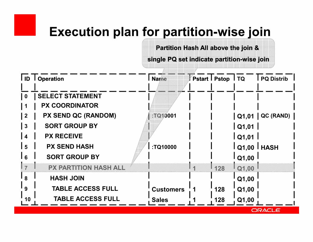
Execution plan for partition-wise join

IDID OperationOperation Name Name PstartPstart PstopPstop TQ PQ Distrib

0 SELECT STATEMENT

1 PX COORDINATOR

2 PX SEND QC (RANDOM) :TQ10001 Q1,01 QC (RAND)

Partition Hash All above the join & Partition Hash All above the join &

single PQ set indicate partitionsingle PQ set indicate partition--wise joinwise join

3 SORT GROUP BY Q1,01

4 PX RECEIVE Q1,01

5 PX SEND HASH :TQ10000 Q1,00 HASH

6 SORT GROUP BY Q1,00

7 PX PARTITION HASH ALL 1 128 Q1,00

8 HASH JOIN Q1,00

9 TABLE ACCESS FULL Customers 1 128 Q1,00

10 TABLE ACCESS FULL Sales 1 128 Q1,00

How Parallel Execution works

User connects to the

database

User

Background process

is spawnedWhen user issues a parallel SQL statement the background process becomes the Query Coordinator

QC gets parallel

servers from global Parallel servers servers from global

pool and distributes

the work to them

Parallel servers -individual sessions that perform work in parallel Allocated from a pool of globally available parallel server processes & assigned to a given operation

Parallel servers communicate among themselves & the QC using messages that are passed via memory

buffers in the shared pool

Query CoordinatorQuery Coordinator

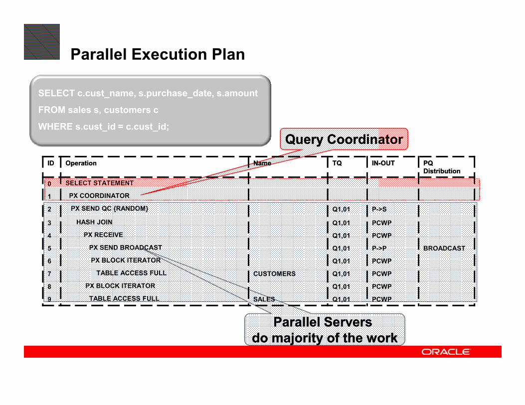
Parallel Execution Plan

IDID OperationOperation Name Name TQTQ ININ--OUTOUT PQ PQ

DistributionDistribution

0 SELECT STATEMENT

1 PX COORDINATOR

SELECT c.cust_name, s.purchase_date, s.amount

FROM sales s, customers c

WHERE s.cust_id = c.cust_id;

Parallel Servers Parallel Servers

do majority of the workdo majority of the work

2 PX SEND QC {RANDOM} Q1,01 P->S

3 HASH JOIN Q1,01 PCWP

4 PX RECEIVE Q1,01 PCWP

5 PX SEND BROADCAST Q1,01 P->P BROADCAST

6 PX BLOCK ITERATOR Q1,01 PCWP

7 TABLE ACCESS FULL CUSTOMERS Q1,01 PCWP


9 TABLE ACCESS FULL SALES Q1,01 PCWP

Parallel Execution of a Query

SELECT c.cust_name, s.date,

s.amount

FROM sales s, customers c

WHERE s.cust_id = c.cust_id;Consumers

Producers

ConsumersConsumersConsumersConsumers Query CoordinatorQuery Coordinator

Producers and Consumer in the execution plan

IDID OperationOperation Name Name TQTQ ININ--OUTOUT PQ PQ

DistributionDistribution

0 SELECT STATEMENT

1 PX COORDINATOR

2 PX SEND QC {RANDOM} Q1,02 P->S

3 HASH JOIN Q1,02 PCWP


ProducersProducersProducersProducers


5 PX SEND HASH Q1,00 P->P


7 TABLE ACCESS FULL CUSTOMERS Q1,00 PCWP


9 PX SEND HASH Q1,01 P->P


11 TABLE ACCESS FULL SALES Q1,01 PCWP

Parallel Execution of a Scan

• Data is divided into Granules

– block range or partition

• Each Parallel Server is assigned one or more Granules

• No two Parallel Servers ever contend for the same Granule

Full scan of the sales table

PQ 1

for the same Granule

• Granules are assigned so that the load is balanced across all Parallel Servers

• Dynamic Granules chosen by the optimizer

• Granule decision is visible in execution plan

PQ 2

PQ 3

Identifying Granules of Parallelism during scans in

the plan

Controlling Parallel Execution on RAC

1. Use RAC Services

Create two services

Srvctl add service –d database_name

-s ETL

-r sid1, sid2

ETL Ad-Hoc queries

Srvctl add service –d database_name

-s AHOC

-r sid3, sid4

2. PARALLEL_FORCE_LOCAL - New Parameter forces parallel statement to run on just node it was issued on Default is FALSE

Use Parallel Execution with common sense

• Parallel execution provides performance boost but requires more resources

• General rules of thumb for determining the appropriate DOP

– objects smaller than 200 MB should not use any parallelism

– objects between 200 MB and 5GB should use a DOP of 4– objects between 200 MB and 5GB should use a DOP of 4

– objects beyond 5GB use a DOP of 32

Mileage may vary depending on concurrent workload and hardware

configuration

Data Loading

Access Methods

Bulk Performance

Data Pump

TTSFlat Files

Heterogeneous

Web Services

DBLinks

XML Files

Data Loading Best Practices

• External Tables

– Allows flat file to be accessed via SQL PL/SQL as if it was a table

– Enables complex data transformations & data cleansing to occur “on the fly”

– Avoids space wastage

• Pre-processing

– Ability to specify a program that the access driver will execute to read the data– Ability to specify a program that the access driver will execute to read the data

– Specify gunzip to decompress a .gzip file “on the fly” while its being

• Direct Path in parallel

– Bypasses buffer cache and writes data directly to disk via multi-block async IO

– Use parallel to speed up load

– Remember to use Alter session enable parallel DML

• Range Partitioning

– Enables partition exchange loads

• Data Compression

SQL Loader or External Tables

• And the winner is => External Tables

• Why:

– Full usage of SQL capabilities directly on the data

– Automatic use of parallel capabilities (just like a table)

– No need to stage the data again

– Better allocation of space when storing data

• High watermark brokering

• Autoallocate tablespace will trim extents after the load

– Interesting capabilities like

• The usage of data pump

• The usage of pre-processing

Tips for External Tables

• File locations and size

– When using multiple files the file size should be similar

– List largest to smallest in LOCATION clause if not similar in size

• File Formats

– Use a format allowing position-able and seek-able scans

– Delimitate clearly and use well known record termination to allow for

automatic Granulationautomatic Granulation

– Always specify the character set if its different to the database

• Consider compressing data files and uncompressing during

loading

• Run all queries before the data load to populate column usage

for histogram creation during statistics gathering

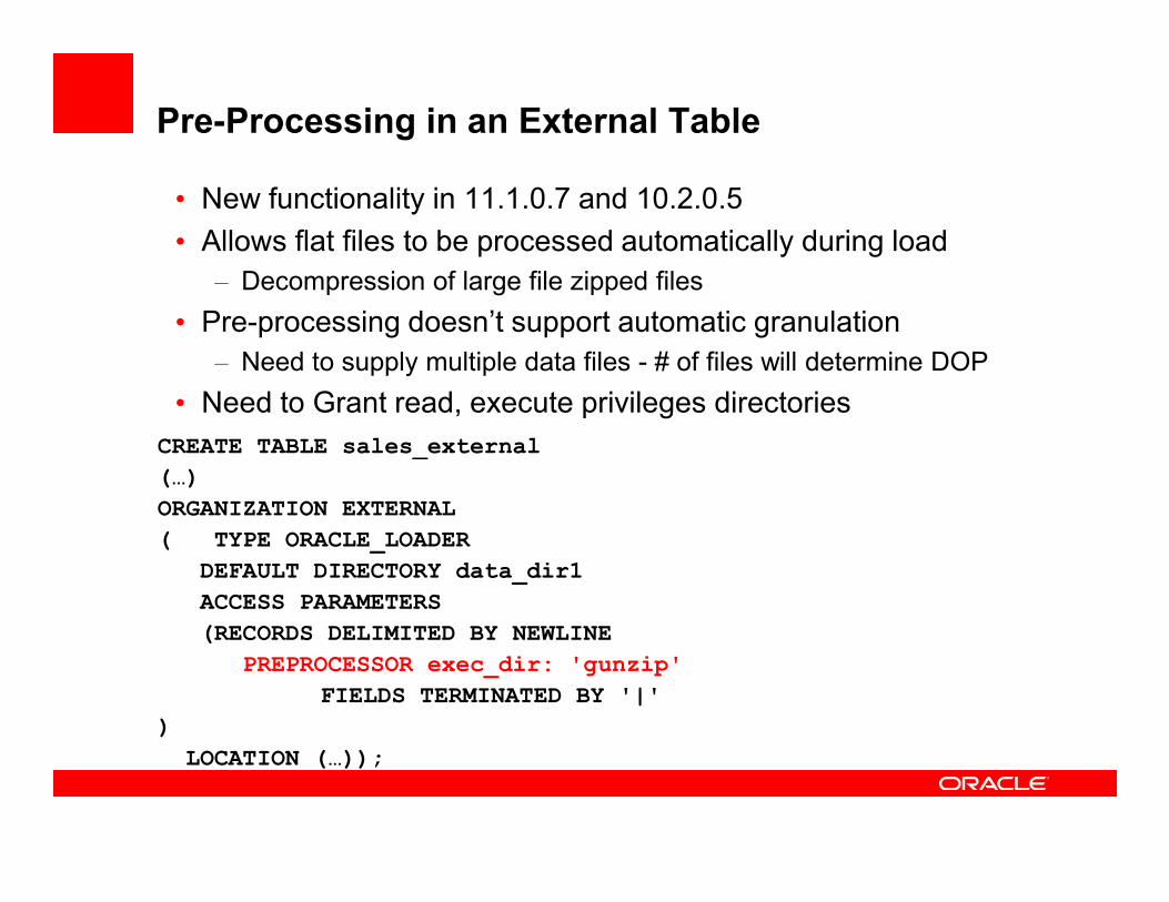
Pre-Processing in an External Table

• New functionality in 11.1.0.7 and 10.2.0.5

• Allows flat files to be processed automatically during load

– Decompression of large file zipped files

• Pre-processing doesn’t support automatic granulation

– Need to supply multiple data files - # of files will determine DOP

• Need to Grant read, execute privileges directories

CREATE TABLE sales_externalCREATE TABLE sales_external

(…)

ORGANIZATION EXTERNAL

( TYPE ORACLE_LOADER

DEFAULT DIRECTORY data_dir1

ACCESS PARAMETERS

(RECORDS DELIMITED BY NEWLINE

PREPROCESSOR exec_dir: 'gunzip'

FIELDS TERMINATED BY '|'

)

LOCATION (…));

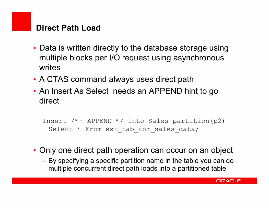
Direct Path Load

• Data is written directly to the database storage using

multiple blocks per I/O request using asynchronous

writes

• A CTAS command always uses direct path

• An Insert As Select needs an APPEND hint to go

directdirect

Insert /*+ APPEND */ into Sales partition(p2)

Select * From ext_tab_for_sales_data;

• Only one direct path operation can occur on an object

– By specifying a specific partition name in the table you can do multiple concurrent direct path loads into a partitioned table

Parallel Load

• Ensure direct path loads go parallel

– Specify parallel degree either with hint or on both tables

– Enable parallelism by issuing alter session command

• CTAS will go parallel automatically when DOP is

specifiedspecified

• IAS will not – it needs parallel DML to be enabled

ALTER SESSION ENABLE PARALLEL DML;

Sales TableSales TableMay 18May 18thth

20082008

May 19May 19thth

20082008

May 20May 20thth

20082008

May 21May 21stst

DBA

1. Create external table

for flat files

2. Use CTAS command

to create non-

Partition Exchange Loading

May 22May 22ndnd

20082008

May 23May 23rdrd

20082008

May 24May 24thth

20082008

May 21May 21stst

20082008to create non-

partitioned table

TMP_SALES

TmpTmp_ sales _ sales

TableTable

4. Alter table Sales

exchange partition

May_24_2008 with table

tmp_sales

May 24May 24thth

20082008

Sales

table now

has all the

data

3. Create indexes

TmpTmp_ sales _ sales

TableTable

5. Gather Statistics

Data Compression

• Use if data being loaded will be read / used more than

once

• Works by eliminating duplicate values within a database

block

• Reduces disk and memory usage, often resulting in

better scale-up performance for read-only operationsbetter scale-up performance for read-only operations

• Require additional CPU during the initial data load

• But what if workload requires conventional DML access

to the data after it has been loaded ?

Use the COMPRESS FOR ALL OPERATIONS

Workload

Monitoring

Statistics gathering

• You must gather optimizer statistics

– Using dynamic sampling is not an adequate solution

• Run all queries against empty tables to populate

column usage

– This helps identify which columns automatically get – This helps identify which columns automatically get

histograms created on them

• Optimizer statistics should be gathered after the data

has been loaded but before any indexes are created

– Oracle will automatically gather statistics for indexes as they

are being created

Statistics Gathering

• By default DBMS_STATS gathers following stats for each table

– global (table level)

– partition level

– Sub-partition

• Optimizer uses global stats if query touches two or more partitions

• Optimizer uses partition stats if queries do partition elimination and • Optimizer uses partition stats if queries do partition elimination and

only one partition is necessary to answer the query

– If queries touch two or more partitions the optimizer will use a combination

of global and partition level statistics

• Optimizer uses sub-partition level statistics if your queries do partition

elimination and only one sub-partition is necessary to answer query

Efficiency Statistics Management

• How do I gather accurate Statistics• “ .. Compute statistics gives accurate results but takes too long ..”

• “ .. Sampling is fast but not always accurate ..”

• “ .. AUTO SAMPLE SIZE does not always work with data skew ..”

•New groundbreaking implementation for AUTO SAMPLE SIZE

•Faster than sampling

•Accuracy comparable to compute statistics

• Gathering statistics on one partition (e.g. after a bulk load)

causes a full scan of all partitions to gather global table

statistics Extremely time and resource intensive

•Use incremental statistics

•Gather statistics for touched partition(s) ONLY

•Table (global) statistics are built from partition statistics

•Accuracy comparable to compute statistics

Incremental Global Statistics


May 18May 18thth

20082008

May 19May 19thth

20082008

May 20May 20thth

20082008

May 21May 21stst

20082008

1. Partition level stats are

gathered & synopsis

created

2. Global stats generated by aggregating partition

synopsis

May 22May 22ndnd

20082008

May 23May 23rdrd

20082008

20082008

Sysaux Tablespace

Incremental Global Statistics Cont’d


May 18May 18thth

20082008

May 19May 19thth

20082008

May 20May 20thth

20082008

May 21May 21stst

20082008

3. A new partition is added to the table & Data is

Loaded

6. Global stats generated by aggregating the original

partition synopsis with the new one

May 22May 22ndnd

20082008

May 23May 23rdrd

20082008

May 24May 24thth

20082008

20082008

Sysaux Tablespace

May 24May 24thth

200820084. Gather partition statistics for new

partition

5. Retrieve synopsis for each of the other

partitions from Sysaux

Step necessary to gather accurate statistics

• Turn on incremental feature for the tableEXEC

DBMS_STATS.SET_TABLE_PREFS('SH’,'SALES','INCREMENTAL','TRUE');

• After load gather table statistics using GATHER_TABLE_STATS

command don’t need to specify many parameter– EXEC DBMS_STATS.GATHER_TABLE_STATS('SH','SALES');

• The command will collect statistics for partitions and update the global

statistics based on the partition level statistics and synopsis

• Possible to set incremental to true for all tables using– EXEC DBMS_STATS.SET_GLOBAL_PREFS('INCREMENTAL','TRUE');

Initialization parameters

Only set what you really need to

Parameter Value Comments

compatible 11.1.0.7.0 Needed for Exadata

db_block_size 8 KB Larger size may help with

compression ratio

db_cache_size 5 GB Large enough to hold metadata

parallel_adaptive_multi_user False Can cause unpredictable response

times as it is based on concurrencytimes as it is based on concurrency

parallel_execution_message_size 16 KB Improves parallel server processes

communication

parallel_min_servers 64 Avoids query startup costs

parallel_max_servers 128 Prevents systems from being

flooded by parallel servers

pga_aggregate_target 18 GB Tries to keep sorts in memory

shared_pool_size 4 GB Large enough to for PX

communicate and SQL Area

Using EM to monitor Parallel Query

Click on the performance

tab

Parallel Execution screens

Click on the SQL

Monitoring link


Click on a SQL ID to drill down to more details

Shows parallel degree used and number of nodes used in query

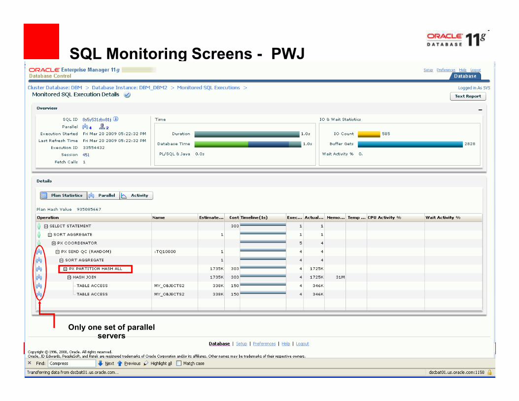
SQL Monitoring Screens - PWJ

Only one set of parallel servers


CoordinatorCoordinator

Producers

Consumers

SQL Monitoring screens

Click on parallel tab to get more

The green arrow indicates which line in the execution plan is currently being worked on

tab to get more info on PQ

SQL Monitoring Screens

By clicking on the + tab you can get more detail about what each individual parallel server is doing. You want to check each slave is

doing an equal amount of work

Disk Configuration with ASM

For More Information

search.oracle.com

Best Practices for Data Warehousing

orhttp://www.oracle.com/technology/products/bi/db/11g/pdf/twp_dw_best_practies_11g11_2008_09.pdf

Exadata SessionsDate Time Room Session Title

Mon

10/12

5:30

PM

Moscone South

307S311436 - Implement Best Practices for Extreme Performance with Oracle Data Warehouses.

Tue

10/13

11:30

AM

Moscone South

307S311385 - Extreme Backup and Recovery on the Oracle Database Machine.

Tue

10/13

1:00

PM

Moscone South

307S311437 - Achieve Extreme Performance with Oracle Exadata and Oracle Database Machine.

Tue

10/13

1:00

PM

Moscone South

Room 102

S311358 - Oracle's Hybrid Columnar Compression: The Next-Generation Compression

Technology

Tue

10/13

2:30

PM

Moscone South

102S311386 - Customer Panel 1: Exadata Storage and Oracle Database Machine Deployments.

Tue

10/13

4:00

PM

Moscone South

102S311387 - Top 10 Lessons Learned Implementing Oracle and Oracle Database Machine.

10/13 PM 102S311387 - Top 10 Lessons Learned Implementing Oracle and Oracle Database Machine.

Tue

10/13

5:30

PM

Moscone South

308S311420 - Extreme Performance with Oracle Database 11g and In-Memory Parallel Execution.

Tue

10/13

5:30

PM

Moscone South

Room 104 S311239 - The Terabyte Hour with the Real-World Performance Group

Tue

10/13

5:30

PM

Moscone South

252S310048 - Oracle Beehive and Oracle Exadata: The Perfect Match.

Wed

10/14

4:00

PM

Moscone South

102S311387 - Top 10 Lessons Learned Implementing Oracle and Oracle Database Machine.

Wed

10/14

5:00

PM

Moscone South

104S311383 - Next-Generation Oracle Exadata and Oracle Database Machine: The Future Is Now.

Thu

10/15

12:00

PM

Moscone South

307

S311511 - Technical Deep Dive: Next-Generation Oracle Exadata Storage Server and Oracle

Database Machine

best practices for extreme performance with oracle data warehousing

Documents