better results are always achieved through teamwork
TRANSCRIPT

UNIVERSITÀ DEGLI
F
CORSO DI
ANNO
OVERVIEW OF THE CASSINI
PROCESSING ALTIMETRIC DATA
Relatore
Prof. Roberto Seu
NIVERSITÀ DEGLI STUDI DI ROMA “L A SAPIENZA
FACOLTÀ DI INGEGNERIA
ORSO DI LAUREA IN INGEGNERIA DELLE
TELECOMUNICAZIONI
NNO ACCADEMICO 2007/2008
LA SAPIENZA
OVERVIEW OF THE CASSINI
PROCESSING ALTIMETRIC DATA
SYSTEM
Oriol Martín
APIENZA”
NGEGNERIA DELLE
OVERVIEW OF THE CASSINI
PROCESSING ALTIMETRIC DATA
Laureando
Oriol Martín Isanda

"better results are always achieved through teamwork"

GENERAL INDEX
3
GENERAL INDEX
1) INTRODUCTION TO THE CASSINI-HUYGENS INTERPLANETARY MISSION TO TITAN 5
1.1) Titan 5
1.2) Overview of the mission 8
1.3) Main Objectives 9
1.4) Spacecraft 10
1.5) The Cassini Radar 13
2) THE CASSINI PROCESSING ALTIMETRIC DATA SYSTEM 18
2.1) Introduction 18
2.2) Data Product Identification 18
2.3) ABDR Production Tool (PT) 21
2.3.A) Input Data Retrieving/Reading. 24
2.3.B) Radar Mode Reading. 30
2.3.C) Range Processing. 30
2.3.D) Intermediate files generation 32
2.3.E) ABDR file generation, file naming, labeling and saving 32
2.4. PAD Science Look Tool (SLT). 33
2.4.A) Input Data Retrieving/Reading 37
2.4.B) Averaging compressed burst 37
2.4.C) Configuration file 39
2.4.D) Surface Parameters Estimation 39
2.4.D.1) Initial Guess Evaluation 41
2.4.D.3) Model Selection 43
2.4.D.4) Impulse Response implementation 48
2.4.D.5) Time Gating functions evaluation 50
2.4.D.6) Roughness gating functions evaluation 52
2.4.D.7) Error evaluation 53
2.4.D.8) Parameters estimation: final considerations 55
2.4.E) Height Retrieval 59
2.4.F) Slope Evaluation 62
2.4.G) Waveform Analysis 62
2.4.H) Performance Simulation 62
2.4.I) Results Workspace Saving 63

GENERAL INDEX
4
3) ANNEXES 64
3.0) Altimetry Radar 64
3.1) Range Processing 68
3.1.1) SNR Maximization 69
3.1.2) Chirp Pulse Compression 70
3.2) MLE structure 74
3.3) Implemented Models 76
3.3.1) Brown’s Model 77
3.3.2) Nadir Model 81
3.3.3) Asymptotic Brown Model 86
3.3.4) Prony’s Method Model 90
3.4) Gating Functions 92
3.4.1) Nadir Model time gating function 92
3.4.2) Asymptotic Brown Model time gating function 93
3.4.3) Prony’s Method Model time gating function 94
3.4.4) Nadir Model roughness gating function 95
3.4.5) Asymptotic Brown Model roughness gating function 95
3.4.6) Prony’s Method Model roughness gating function 96
3.5) Prony’s Method 96
3.6) Doppler Tracking 98
CONCLUSIONS 100
BIBLIOGRAPHY 102

CHAPTER 1. INTRODUCTION TO THE CASSINI-HUYGENS INTERPLANETARY MISSION TO TITAN
5
1) INTRODUCTION TO THE CASSINI-HUYGENS
INTERPLANETARY MISSION TO TITAN
Although the Cassini-Huygens interplanetary mission is a project that covers Saturn, its
rings and most of its multiple satellites, in this introduction attention will be focused
mainly in the biggest moon of Saturn: Titan, since Cassini Radar, from which Cassini
Processing Altimetric Data (PAD) system (on which is based this work) receives science
data, has been built especially to study Titan.
1.1) Titan
Saturn, being the second outer planet of the solar system has a large number of
satellites. The largest saturnine satellites known before the start of space research
were: Mimas, Encélado, Tethys, Dione, Rea, Titan, Hyperion, Jápeto and Febe.
Titan is the largest of them and the second largest satellite in the whole Solar System,
after Jupiter’s moon Ganymede. It was discovered on March 25, 1655 by Dutch
astronomer Christiaan Huygens, and was the first
satellite in the Solar System to be discovered after
Jupiter’s Galilean moons. Titan has a 5.150 km diameter,
and is larger than planets Mercury (although only half as
massive) and Pluto. It orbits Saturn at a distance of
1,222,000 km and it takes 15.9 days to complete an
entire revolution.
Moreover Titan is the only moon in the solar system that
has a significant atmosphere. The presence of this
atmosphere was proposed by the Catalan astronomer
Jose Comas and Solá in 1908 based on his observations
of Titan’s darkening towards the edge of its disc. Before
the arrival of Voyager 1 in 1980, Titan was thought to be
slightly larger than Ganymede (diameter 5,262 km) and thus the largest moon in the
Solar System; this was an overestimation
caused by Titan's dense, opaque
atmosphere which extends many miles
above its surface and increases its
apparent diameter.
The atmosphere of Titan dense, orange,
and rich in methane and other
hydrocarbons (1.6%), is other than that of
Earth, the only which is mainly composed
of nitrogen (98.4%). It is opaque at many
wavelengths and a complete reflectance
spectrum of the surface is impossible to acquire from the outside and that made that
Image 2. Titan compared to Earth
Image 1. Titan's orbit (highlighted
in red) among the other large
inner moons of Saturn.

CHAPTER
before the Cassini mission, information and maps from Titan’s surface were
inaccurate. Its chemical com
atmosphere of the Earth in prebiotic times. Temperatures of about 90K should have
preserved a very similar environment to that of the primitive Earth although at a much
lower temperature. The atmosphere of
atmosphere. Titan's surface
instead be reflecting off the liquid
The surface is geologically young; although mountains and several possible
cryovolcanoes have been discovered.
smooth (and thus dark to radar) patches were seen dotting the surface near the pole.
Based on the observations, scientists announced "definitive evidence of lakes filled
with methane on Saturn's moon Titan" in January 2007.
Image 4. False-color Cassini synthetic
of Titan's north polar region, showing evidence for
hydrocarbon seas, lakes and tributary networks.
Image 3. Titan's internal structure
HAPTER 1. INTRODUCTION TO THE CASSINI-HUYGENS INTERPLANETARY MISSIO
mission, information and maps from Titan’s surface were
Its chemical composition seems to be very similar to the primitive
atmosphere of the Earth in prebiotic times. Temperatures of about 90K should have
preserved a very similar environment to that of the primitive Earth although at a much
lower temperature. The atmosphere of Titan is denser than that of the Earth, with a
surface pressure about one and a half times
higher than that of our planet and with an
opaque cloud layer formed by hydrocarbon
aerosols that hide the features of Titan’s
surface.
Titan is primarily composed of water ice and
rocky material and is probably differentiated
into several layers with a 3,400
center surrounded by several layers composed
of different crystal forms of ice. Its interior
may still be hot and there may be a liquid layer
consisting of water and ammonia
ice crust and deeper ice layers made of
high-pressure forms of ice. Evidence for such
an ocean has recently been uncovered by the
Cassini probe in the form of natural
low frequency (ELF) radio waves in Titan's
atmosphere. Titan's surface is thought to be a poor reflector of ELF waves, so they may
instead be reflecting off the liquid-ice boundary of a subsurface ocean.
The surface is geologically young; although mountains and several possible
have been discovered. Through images obtained with the Hubble Space
Telescope a strange region,
unofficially named Xanadu was
discovered in 1994, with an area
about the size of Australia,
other dark areas of similar size
elsewhere on the moon and it had
been speculated that these are
methane or ethane seas.
mission affirmed the former
hypothesis: at Titan's south pole, an
enigmatic dark feature named
Ontario Lacus was the first suspected
lake identified. Following a flyby on
July 22, 2006, in which th
spacecraft's radar imaged the
northern latitudes, a number of large,
smooth (and thus dark to radar) patches were seen dotting the surface near the pole.
Based on the observations, scientists announced "definitive evidence of lakes filled
thane on Saturn's moon Titan" in January 2007.
color Cassini synthetic-aperture radar mosaic
of Titan's north polar region, showing evidence for
hydrocarbon seas, lakes and tributary networks.
NTERPLANETARY MISSION TO TITAN
6
mission, information and maps from Titan’s surface were
position seems to be very similar to the primitive
atmosphere of the Earth in prebiotic times. Temperatures of about 90K should have
preserved a very similar environment to that of the primitive Earth although at a much
Titan is denser than that of the Earth, with a
surface pressure about one and a half times
higher than that of our planet and with an
opaque cloud layer formed by hydrocarbon
aerosols that hide the features of Titan’s
ed of water ice and
rocky material and is probably differentiated
into several layers with a 3,400 km rocky
center surrounded by several layers composed
of different crystal forms of ice. Its interior
may still be hot and there may be a liquid layer
ammonia between the
crust and deeper ice layers made of
pressure forms of ice. Evidence for such
n ocean has recently been uncovered by the
probe in the form of natural extremely
(ELF) radio waves in Titan's
is thought to be a poor reflector of ELF waves, so they may
The surface is geologically young; although mountains and several possible
Through images obtained with the Hubble Space
Telescope a strange region,
unofficially named Xanadu was
discovered in 1994, with an area
about the size of Australia, there are
of similar size
elsewhere on the moon and it had
been speculated that these are
methane or ethane seas. The Cassini
mission affirmed the former
hypothesis: at Titan's south pole, an
enigmatic dark feature named
was the first suspected
lake identified. Following a flyby on
, in which the Cassini
spacecraft's radar imaged the
northern latitudes, a number of large,
smooth (and thus dark to radar) patches were seen dotting the surface near the pole.
Based on the observations, scientists announced "definitive evidence of lakes filled

CHAPTER 1. INTRODUCTION TO THE CASSINI-HUYGENS INTERPLANETARY MISSION TO TITAN
7
In Titan, methane plays the role of water on Earth; it produces clouds in its
atmosphere that, when they condense on the aerosols, produce a methane rain with
particles that fill the streams with a dark flowing material. Therefore rain, along with
wind, creates surface features that are
similar to those on Earth, such as sand
dunes, shorelines, seas, lakes and rivers
and, like Earth, is dominated by seasonal
weather. Thus Titan is the only known
object other than Earth in the Solar System
where it rains on the surface and for which
clear evidence of stable bodies of surface
liquid has been found.
Titan's surface temperature is about 94 K
(−179 °C, or −290 °F). At this temperature
water ice does not sublimate from solid to
gas, so the atmosphere is nearly free of
water vapor. The haze in Titan's
atmosphere contributes to the moon's anti-
greenhouse effect by reflecting sunlight away from the satellite, making its surface
significantly colder than its
upper atmosphere.
The clouds on Titan, composed
of methane, ethane or other
simple organics, are scattered
and variable, punctuating the
overall haze. This atmospheric
methane conversely creates a
greenhouse effect on Titan's
surface, without which Titan
would be far colder. The
findings of the Huygens probe
indicate that Titan's
atmosphere periodically rains
liquid methane and other
organic compounds onto the
moon's surface.
With Cassini-Huygens interplanetary mission, scientists hope to reach a better
understanding of the surface, atmosphere and chemical composition of Titan to
perhaps shed some light on how Earth might have been before life, as we know it,
began to pump oxygen into the earth’s atmosphere.
Image 6. A graph detailing temperature, pressure, and other
aspects of Titan's atmosphere.
Image 5. Sand dunes on Earth (top), compared with
dunes on Titan's surface.

CHAPTER 1. INTRODUCTION TO THE CASSINI-HUYGENS INTERPLANETARY MISSION TO TITAN
8
1.2) Overview of the mission
The Cassini-Huygens is a joint NASA, European Space Agency (ESA), and Italian Space
Agency (ASI) spacecraft interplanetary mission. The total cost of the mission is about
US$3,2 billion, NASA contributed with $2,6 billion, ESA with $500 million and $160
million came from the ASI. The
project proceeded politically
smoothly after 1994, although,
citizens' groups concerned about
its potential environmental
impact attempted to derail it
through protests and lawsuits
until and past its 1997 launch. A
few years after being approved
by the United States Congress
and after an intensive work of
design, development and seek of
international cooperation the
spacecraft was ready for its
launch from the Kennedy Space
Center on October 15th, 1997.
The spacecraft entered into orbit
around Saturn on July 1, 2004
after giving two laps around the Sun and having taken advantage of the gravitational
field of Venus, Earth and Jupiter to achieve enough momentum to reach the outer
Solar System, using a new technique known as "gravity assists" whereby the spacecraft
"steals" a small part of the planet’s orbital energy. This technique came about in
response to the fact that
no existing launcher could
have sent, with enough
power, the 6000 kg.
spacecraft directly to
Saturn.
The Cassini-Huygens
spacecraft was composed
of the Cassini orbiter,
designed to orbit Saturn
and its moons for four
years and which is doing
so since the July 1, 2004,
and the Huygens probe
that was separated from the orbiter on December 25, 2004 and arrived at the surface
of Titan on 14 January 2005, successfully fulfilling its mission to descend over Titan's
atmosphere collecting all kind of information along the way, and finally to land on
Titan’s surface, analyzing it and then sending the data to the Cassini orbiter.
Image 7. Orbital motion of Cassini–Huygens on and after arrival
at Saturn.
Image 8. Initial gravity-assist trajectory of Cassini–Huygens.

CHAPTER 1. INTRODUCTION TO THE CASSINI-HUYGENS INTERPLANETARY MISSION TO TITAN
9
The Cassini orbiter was built and managed by NASA/Caltech's Jet Propulsion
Laboratory. The Huygens probe was built by the European Space Agency (ESA). The
Italian Space Agency (ASI) provided Cassini's high-gain communication antenna, and a
revolutionary compact and light-weight multimode radar (synthetic aperture radar,
radar altimeter, radiometer).
During the 4 years the Cassini is orbiting Saturn is expected to submit enough
information to understand and study in detail the planet and its magnetosphere, its
rings and its numerous natural satellites. The nominal end of the mission is in 2008 but
an extension to the mission is being planned which will end in 2010, although this has
yet to be formally announced.
1.3) Main Objectives
The main objectives of the mission are:
- For Saturn:
• Determine the temperature field, cloud properties and composition of Saturn's
atmosphere.
o Image Saturn's atmosphere over a large range of latitudes and
longitudes.
o Determine the 2-cm wavelength radiometer thermal emission from the
subcloud atmosphere.
o Study belt/zone structure variations in ammonia concentration.
• Measure the planet's global wind field, including its waves; make long-term
observations of cloud features to see how they grow, evolve, and dissipate.
• Determine the internal structure and rotation of the deep atmosphere.
o Explore the unknown dynamical properties of the atmosphere.
o Examine ammonia as a tracer for atmospheric circulations.
o Determine the equator-to-pole temperature gradient and unknown
subcloud longitudinal structures.
• Study daily variations and relationship between the ionosphere and the
planet's magnetic field.
• Determine the composition, heat flux, and radiation environment present
during Saturn's formation and evolution.
• Investigate sources and nature of Saturn's lightning.
- For the Rings:
• Study configuration of the rings and dynamic processes responsible for ring
structure.
• Map the composition and size distribution of ring material.

CHAPTER 1. INTRODUCTION TO THE CASSINI-HUYGENS INTERPLANETARY MISSION TO TITAN
10
• Investigate the interrelation of Saturn's rings and moons, including imbedded
moons.
• Determine the distribution of dust and meteoroid distribution in the vicinity of
the rings.
• Study the interactions between the rings and Saturn's magnetosphere,
ionosphere and atmosphere.
- For Titan:
• Determine the most abundant elements, and most likely scenarios for the
formation and evolution of Titan and its atmosphere.
• Determine the relative amounts of different components of the atmosphere
• Observe vertical and horizontal distributions of trace gases; search for complex
molecules; investigate energy sources for atmospheric chemistry; determine
the effects of sunlight on chemicals in the stratosphere; study formation and
composition of aerosols (particles suspended in the atmosphere).
• Measure winds and global temperatures; investigate cloud physics, general
circulation and seasonal effects in Titan's atmosphere; search for lightning.
• Determine the physical state, topography and composition of Titan's surface;
characterize its internal structure.
• Investigate Titan's upper atmosphere, its ionization and its role as a source of
neutral and ionized material for the magnetosphere of Saturn.
• Determine whether Titan's surface is liquid or solid; analyze the evidence of a
bright continent as indicated in Hubble images taken in 1994.
1.4) Spacecraft
Cassini-Huygens is one of the most ambitious missions ever launched into space.
Loaded with an array of powerful instruments and cameras, the spacecraft is capable
of taking accurate measurements and detailed images in a variety of atmospheric
conditions and light spectra.
The spacecraft, including the orbiter and the probe, is the largest and most complex
interplanetary spacecraft built to date. The orbiter has a mass of 2,150 kg, the probe
350 kg. With the launch vehicle adapter and 3,132 kg of propellants at launch, the
spacecraft had a mass of about 5,600 kg. Only the two Phobos spacecraft sent to Mars
by the Soviet Union were heavier. The Cassini spacecraft was more than 6.8 meters
(22.3 ft) high and more than 4 meters (13.1 ft) wide. The complexity of the spacecraft
is necessitated both by its trajectory (flight path) to Saturn, and by the ambitious
program of scientific observations once the spacecraft reaches its destination.

CHAPTER 1. INTRODUCTION TO THE CASSINI-HUYGENS INTERPLANETARY MISSION TO TITAN
11
Cassini-Huygens is a three-axis stabilized
spacecraft equipped for 27 diverse science
investigations. The Cassini orbiter has 12
instruments and the Huygens probe had six. The
instruments often have multiple functions,
equipped to thoroughly investigate all the
important elements that the Saturn system may
uncover. The spacecraft communicates through
one high-gain and two-low gain antennas. It is
only in the event of a power failure or other such
emergency situation, however, that the
spacecraft will communicate through one of its
low-gain antennas, known as LGA-1.
Three Radioisotope Thermoelectric Generators
(commonly referred to as RTGs) provide power
for the spacecraft, including the instruments,
computers, and radio transmitters on board,
attitude thrusters, and reaction wheels.
- Cassini orbiter instruments:
• Optical Remote sensing. Mounted on the remote sensing pallet, these
instruments study Saturn and its rings and moons in the electromagnetic
spectrum.
o Composite Infrared Spectrometer (CIRS). the Composite Infrared
Spectrometer consists of a dual interferometer, which measures the
infrared emission from atmospheres, rings and surfaces at wavelengths
between 7 and 1000 microns to determine their composition and
temperatures.
o Imaging Science Subsystem (ISS). the scientific imaging subsystem is a
remote sensor that captures images in visible light, infrared and
ultraviolet. The science objectives include studying the atmospheres of
Saturn and Titan, Saturn's rings and their interactions with the satellites
of the planet and the characteristics of the satellites, including Titan.
o Ultraviolet Imaging Spectrograph (UVIS). is a set of detectors designed
to measure ultraviolet light reflected or emitted by atmospheres, rings
and surfaces to determine its composition, distribution, aerosol content
and temperatures.
o Visible and Infrared Mapping Spectrometer (VIMS). is a remote sensor
consisting of two cameras in one: one is used for measurements in the
visible spectrum and the other infrared.
o The VIMS obtains images using infrared light and visible to learn more
about the composition of the lunar surface, rings and atmospheres of
Saturn and Titan.
Image 9. Cassini Spacecraft

CHAPTER 1. INTRODUCTION TO THE CASSINI-HUYGENS INTERPLANETARY MISSION TO TITAN
12
• Fields, Particles and Waves. These instruments study the dust, plasma and
magnetic fields around Saturn. While most don't produce actual "pictures," the
information they collect is critical to scientists' understanding of this rich
environment.
o Cassini Plasma Spectrometer (CAPS). It measures the energy and electric
charge of particles such as electrons and protons that the instrument
founds around the ship. The instrument is used to study the
composition, density, flow, velocity and temperature of ions and
electrons in the magnetosphere of Saturn.
o Cosmic Dust Analyzer (CDA). The Cosmic Dust Analyzer is a direct
instrument sensor that measures the size, speed and direction of dust
particles near Saturn. Some of these particles are orbiting Saturn while
others may come from other solar systems. The CDA on board the
Cassini is designed to help discover more about these mysterious
particles.
o Ion and Neutral Mass Spectrometer (INMS). It is a direct sensor that
analyzes the charged particles (protons and heavy ions) and neutral
particles (atoms) near Titan and Saturn to learn more about their
atmospheres. One of its main aims will be to investigate the interaction
between the upper atmosphere of Titan with the magnetosphere and
the solar wind.
o Magnetometer (MAG). It is a direct sensor that measures the strength
and direction of the magnetic field around Saturn. The information
collected by MAG can be used to explain the fact that despite the
magnetic field of Saturn is similar to that of the Earth; the geographic
north pole coincides exactly with the magnetic north pole, which only
happens on this planet throughout the solar system.
o Magnetospheric Imaging Instrument (MIMI). It is a remote and direct
sensor that gets images and other data about the particles trapped in
the large magnetic field of Saturn, and in its magnetosphere. This
information will be used to study the overall configuration and the
dynamics of the magnetosphere and its interactions with the solar wind,
the atmosphere of Saturn, Titan, the rings and the icy satellites.
o Radio and Plasma Wave Science (RPWS). The main functions of the
scientific instrument Wave Radio and Plasma (RWPS) are measuring
electrical and magnetic fields and the electron density and temperature
in the interplanetary medium and planetary magnetospheres.
The scientific instrument of radio waves and plasma (RPWS) will be used
to investigate electric and magnetic waves in space plasma in Saturn.
• Microwave Remote Sensing. Using radio waves, these instruments map
atmospheres, determine the mass of moons, collect data on ring particle size,
and unveil the surface of Titan.
o Radio Science (RSS). It is a remote sensor that uses radio antennas on
Earth to explore how the radio signals from the spacecraft change when

CHAPTER 1. INTRODUCTION TO THE CASSINI-HUYGENS INTERPLANETARY MISSION TO TITAN
13
they are sent through objects such as Titan's atmosphere and the rings
of Saturn.
o Radar. It is both active and passive remote sensor that will produce
maps of the surface of Titan and will measure the height of surface
objects (such as mountains and canyons). In the following paragraphs it
will be described with more detail.
1.5) The Cassini Radar
The main objective of the Cassini Radar Mission is Titan coverage. In order to study
the inaccessible surface of Titan, its proprieties and processes, the spacecraft is
making a number of close flybys, during which, the Cassini Radar conduct intense
observations, in order to achieve its scientific goals. The first targeted fly-by of Titan
(Ta) occurred on Tuesday, October 26, 2004 at 15:30 UTC.
• RADAR Scientific Objectives:
o To determine whether oceans exist on Titan, and, if so, to determine
their distribution.
o To investigate the geologic features and topography of the solid surface
of Titan.
o To acquire data on non-Titan targets (rings, icy satellites) as conditions
permit.
• RADAR Sensing Instruments:
o Synthetic Aperture Radar Imager [SAR] (13.78 GHz Ku-band; 0.35 to 1.7
km resolution).
o Altimeter (13.78 GHz Ku-band; 24 to 27 km horizontal, 90 to 150 m
vertical resolution).
o Radiometer (13.78 GHz passive Ku-band; 7 to 310 km resolution).
• RADAR Instrument Characteristics:
o Mass (current best estimate) = 41.43 kg.
o Peak Operating Power (current best estimate) = 108.40 W.
o Peak Data Rate (current best estimate) = 364.800 kilobits/sec.
The Cassini Radar is a multimode microwave instrument that uses the 4 m high gain
antenna (HGA) onboard the Cassini orbiter. The instrument operates at Ku-band
(13.78 GHz or 2.2 cm wavelength) and is designed to operate in four observational
modes (Imaging, Altimetry, Backscatter and Radiometry) at spacecraft altitude below
100.000 Km, on both inbound and outbound tracks of each hyperbolic Titan flyby, and
to operate over a wide range of geometries and conditions. The instrument has been
designed to have a wide range of capabilities in order to encompass a variety of
possible surface proprieties.

CHAPTER 1. INTRODUCTION TO THE CASSINI-HUYGENS INTERPLANETARY MISSION TO TITAN
14
Between 100.000km and 25.000km
the RADAR will operate exclusively
in the radiometry mode. In this
mode, the RADAR will operate as a
passive instrument, simply recording
the energy emanating from the
surface of Titan. This information
will tell scientists the amount of
latent heat (i.e. moisture) in the
moon's atmosphere, a factor that
has an impact on the precision of
the other measurements taken by
the instrument.
Between 25.000km and 9.000km the radar will operate alternatively as a radiometer
and as a scatterometer (backscatter mode). In the backscatter mode it will bounce
pulses off Titan's surface and then measure the intensity of the energy returning. This
returning energy or backscatter is always less than the original pulse, because surface
features inevitably reflect the pulse in more than one direction. From the backscatter
measurements, scientists can infer the backscattering coefficient �� of the surface of
Titan.
For altitudes less than 4.000km the radar will operate in the imaging mode and
secondarily as a radiometer. In the imaging mode of operation, the RADAR instrument
will bounce pulses of microwave energy off the surface of Titan from different
incidence angles and record the time it takes the pulses to return to the spacecraft.
These measurements, when converted to distances (by dividing by the speed of light),
will allow the construction of visual images of the target surface.
Figure 1.1 Modes of operation of the Cassini Radar for the different S/C altitudes during each fly-by
For altitudes between 9000km and 4000km the radar will operate as a radiometer and
as an altimeter. The Altimeter Mode (ALT) is intended to study the relative topographic
change of Titan’s surface along sub-satellite tracks. The topography is a key
characteristic of planetary surfaces and its quantitative evaluation is essential to
understand flow such as occurs in volcanic and fluvial processes as well as for
Image 10. Spacecraft's High Gain Antenna
CHAPTER 1. INTRODUCTION TO THE CASSINI-HUYGENS INTERPLANETARY MISSION TO TITAN
15
geophysical probing of the interior of planets. Up to now, the only information
about Titan’s topography were from the Voyager-1 radio occultation experiment and
ground based observations. Radar is presently the primary means of determining
topography on Titan, since a smoggy haze completely obscures the satellite’s
surface.
The ALT mode is planned to operate at S/C altitudes between 4000 and 9000 Km,
approximately from 16 minutes before the closest Titan approach of each Titan flyby
until 16 minutes after the closest encounter. The Altimeter operates on “burst mode”,
similar to the imaging mode. When the ALT mode is executed, bursts of frequency
modulated pulse signals (chirp pulses) of 150 µs time duration and at 5 MHz
bandwidth will be transmitted in a Burst Period (the Burst Repetition Interval is 3333
ms). The transmit time varies from 1.4 to 1.8 µs. The number of pulses transmitted in
each burst will vary throughout a single flyby pass.
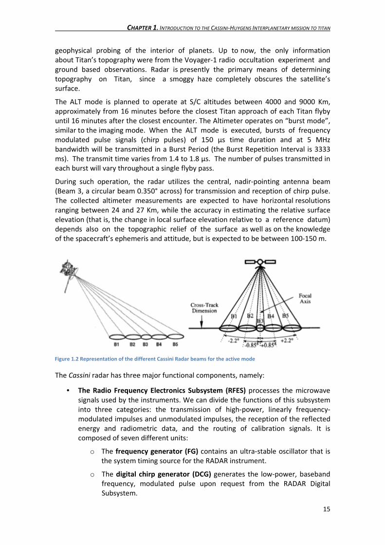
During such operation, the radar utilizes the central, nadir-pointing antenna beam
(Beam 3, a circular beam 0.350° across) for transmission and reception of chirp pulse.
The collected altimeter measurements are expected to have horizontal resolutions
ranging between 24 and 27 Km, while the accuracy in estimating the relative surface
elevation (that is, the change in local surface elevation relative to a reference datum)
depends also on the topographic relief of the surface as well as on the knowledge
of the spacecraft’s ephemeris and attitude, but is expected to be between 100-150 m.
The Cassini radar has three major functional components, namely:
• The Radio Frequency Electronics Subsystem (RFES) processes the microwave
signals used by the instruments. We can divide the functions of this subsystem
into three categories: the transmission of high-power, linearly frequency-
modulated impulses and unmodulated impulses, the reception of the reflected
energy and radiometric data, and the routing of calibration signals. It is
composed of seven different units:
o The frequency generator (FG) contains an ultra-stable oscillator that is
the system timing source for the RADAR instrument.
o The digital chirp generator (DCG) generates the low-power, baseband
frequency, modulated pulse upon request from the RADAR Digital
Subsystem.
Figure 1.2 Representation of the different Cassini Radar beams for the active mode

CHAPTER 1. INTRODUCTION TO THE CASSINI-HUYGENS INTERPLANETARY MISSION TO TITAN
16
o The chirp up-converter and amplifier (CUCA) converts the baseband
chirp pulse to Ku band.
o The high-power amplifier (HPA) receives a low-power Ku-band chirp
pulse from the CUCA and amplifies that pulse to the required power
level for transmission.
o The purpose of the front-end electronics (FEE) is to route the high-
power transmission pulses, the returning low-energy echoes and
radiometric signals, and the calibration signals.
o The microwave receiver (MR) receives signals at Ku band and down-
converts these to baseband so that they can be properly sampled. The
sources of these signals are the echo returns, radiometric signals, and
calibration signals routed through the FEE.
o The RFES power supply converts the (approximately) 30-volt d.c. input
from the Power and Pyrotechnic Subsystem to the required voltages for
the RFES.
• The RADAR Digital Subsystem (DSS) is a central control unit for the RADAR
operations. It manages the switches between the different operation modes
and controls the chirp generation. It receives and transmits the RADAR
commands to the Command and Data Subsystem (CDS), it generates and
controls the properties of the transmitted impulse and manages the transfer of
data and scientific information to the CDS. The DSS consists of the following
units:
o The bus interface unit (BUI) is the interface between RADAR and the
CDS.
o The flight computer unit (FCU) receives and routes the commands, it
controls the RADAR configuration and the CTU information, etc….
o The purpose of the control and timing unit (CTU) is to control the
hardware configuration and the timing of control signals within RADAR.
o The signal conditioner unit (SCU) consists of a science data buffer and
high- and low-speed analog-to-digital (A/D) converters.
o The DSS power supply converts the (approximately) 30-volt d.c. input
from the Power and Pyrotechnic Subsystem to the voltages required for
the DSS.
• The RADAR Energy Storage Subsystem (ESS) converts the (approximately) 30-
volt d.c. input from the PPS to a higher voltage, stores energy in a capacitor
bank, and provides a regulated voltage to the high-power amplifier (HPA) of the
RFES. It is composed by:
o The boost circuitry increases the (approximately) 30-volt d.c. input
power to approximately 85 volts d.c. for more efficient energy storage
by the capacitor bank.
o The capacitor bank stores energy to supply to the buck regulator (and
the HPA) during RADAR pulse bursts.

CHAPTER
o The buck regula
HPA.
Figure 1.3 Block diagram
HAPTER 1. INTRODUCTION TO THE CASSINI-HUYGENS INTERPLANETARY MISSIO
buck regulator regulates the varying capacitor bank voltage for the
Block diagram of the Cassini Titan Radar Mapper
NTERPLANETARY MISSION TO TITAN
17
regulates the varying capacitor bank voltage for the

CHAPTER 2. THE CASSINI PROCESSING ALTIMETRIC DATA SYSTEM
18
2) THE CASSINI PROCESSING ALTIMETRIC DATA SYSTEM
2.1) Introduction
In the frame of CASSINI-HUYGENS interplanetary mission, the Cassini PAD System
contains the HW and SW tools necessary to:
• process the LBDR data (given by JPL � Jet Propulsion Laboratory in Pasadena,
California) in order to produce ABDR science data (a complete overview of the
Cassini PAD data is presented in the following section).
• evaluate the performance of RADAR altimeter.
• produce digital maps of Titan by using data acquired by all Cassini passes.
The Cassini Radar PAD system is conceived to receive science data acquired from the
Cassini Radar while operating in high-resolution altimeter mode (ALTH/AHAG), to
process this data at different levels, archive them, and visualize the obtained products.
The Cassini PAD System shall provide a set of three tools for data processing and
visualization together with the necessary archiving facility. The following Cassini PAD
tools are foreseen:
- ABDR Production Tool (PT): this tool shall be for produce altimetry data by
processing the BODP coming from the Cassini RADAR. It shall take the LBDR files as
input, returning the ABDR files as output.
- PAD Science Look Tool (SLT): this tool shall allow users to interact with
processed data. This tool shall be able to read and to manipulate the Cassini data.
- PAD Map Tool (MT): this tool shall be able to visualize Titan-referenced
altimetry data, with related satellite ground tracks for each Titan fly-by, inferred
surface parameters and all those information which could be of interest through
interaction with a high-resolution Titan map, available in a user-defined projection.
This work will be focused mainly in PT and SLT tools.
Each tool, developed in a Matlab® environment, is provided with a user-friendly
graphical interface (GUI � Graphical User Interface), which allows users to exploit all
implemented functionalities.
2.2) Data Product Identification
Three different types of data products are used by the Cassini Radar:
• Basic Image Data Records (BIDRs).
• Burst Ordered Data Products (BODPs).
• Digital Map Products (DMPs).
The interest of the Cassini Radar PAD system is for Burst Ordered Data Products
(BODPs) which are comprehensive data files that include engineering telemetry, radar

CHAPTER 2. THE CASSINI PROCESSING ALTIMETRIC DATA SYSTEM
19
operational parameters, raw echo data, instrument viewing geometry, and calibrated
science data.
The BODP files contain time-ordered fixed length records. Each record corresponds to
the full set of relevant data for an individual radar burst. The Cassini Radar is operated
in "burst mode", which means the radar transmits a number of pulses in sequence
then waits to receive the return signals. "Burst" is a descriptive term for the train of
pulses transmitted by the radar.
The term "burst" (somewhat unconventionally) is used to refer to an entire
measurement cycle including transmit, receipt of echo, and radiometric (passive)
measurements of the naturally occurring radiation emitted from the surface. Burst
Ordered Data Products are fixed header length, fixed record length files. The header is
an attached PDS label.
The BODP comprise three separate data sets:
• Short Burst Data Record (SBDR).
• Long Burst Data Record (LBDR).
• Altimeter Burst Data Record (ABDR).
The only difference between the three formats is whether or not two data fields are
included: the sampled echo data, and the altimeter profile. The altimeter profile is an
intermediate processing result between sampled echo data and a final altitude
estimate. LBDRs include the echo data but not the altimeter profile. ABDRs include the
altimeter profile but not the echo data. SBDRs include neither.
The SBDR data record is divided into three consecutive segments from three different
levels of processing:
1) The engineering data segment includes a copy of the radar telemetry
contained in the Engineering Ground Support Equipment (EGSE) files obtained from
the spacecraft data downlinks. This data is stored to allow investigators to access as
much of the information obtained by the spacecraft as possible.
2) The intermediate level data segment containing timing and spacecraft
geometry information. The data fields in this segment include time at start of burst,
Figure 2.1 Example of burst cycle time

CHAPTER 2. THE CASSINI PROCESSING ALTIMETRIC DATA SYSTEM
20
spacecraft position and velocity, the direction vectors of the axes of the spacecraft
coordinate system, and the angular velocity vector of the spacecraft.
3) The science data segment: three primary estimates of geophysical quantities
are available in the science data segment:
• the normalized backscatter cross-section �� obtained from the scatterometer
measurement.
• the antenna temperature determined from the radiometer measurement.
• the range to target (RTT = distance between the sensor and the closest surface
point) computed from the altimeter measurement.
In addition to these primary values additional ancillary parameters are also computed.
The ancillary parameters include intermediate values, (e.g., receiver temperature, total
echo energy, system gain, etc.) analytical estimates of the standard deviation of the
residual error in each of the three primary measurements, and measurement
geometry. Synthetic Aperture Radar (SAR) ancillary data is also included in the science
data segment when available.
Engineering
data segment
Intermediate level
data segment
Science data
segment
Sampled echo
data
Altimeter
Profile
Figure 2.2 Structure of the Cassini BODP's files
- Sampled Echo Data:
The sampled echo data array is located at the end of each record in the LBDR data
files. It constitutes the only difference between SBDR records and LBDR records.
The array consists of 32,768 4-byte floating point values. It contains the active mode
time-sampled data obtained during the receive window. The data was encoded prior
to downlinking from the spacecraft in order to minimize the data transfer rate, and
then decoded during the ground processing (the data stored in the array has already
been decoded).
The length of the array corresponds to the maximum amount of echo data that can
ever be obtained from a single burst. Only the first N elements in the array are valid
data. These data are N floating point values in the range [-127.5, 127.5] sampled
SBDR File
LBDR File
ABDR File
CHAPTER 2. THE CASSINI PROCESSING ALTIMETRIC DATA SYSTEM
21
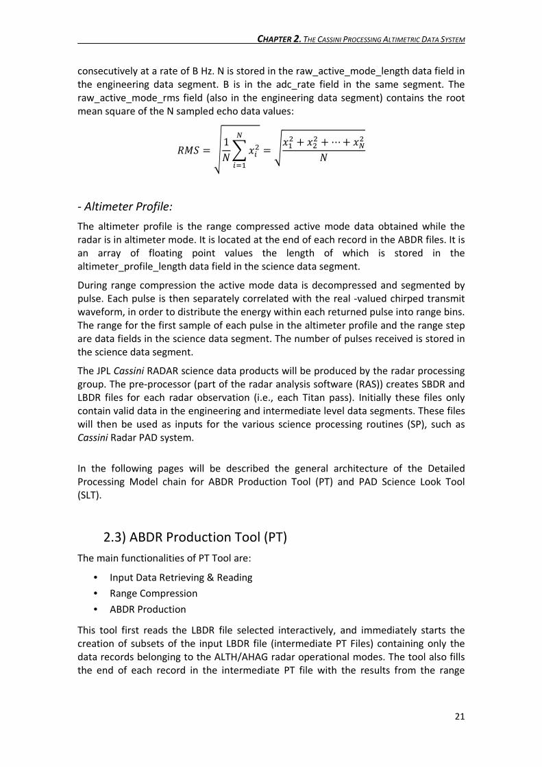
consecutively at a rate of B Hz. N is stored in the raw_active_mode_length data field in
the engineering data segment. B is in the adc_rate field in the same segment. The
raw_active_mode_rms field (also in the engineering data segment) contains the root
mean square of the N sampled echo data values:
��� � �1�� ���� � ��� � � ��� ��
- Altimeter Profile:
The altimeter profile is the range compressed active mode data obtained while the
radar is in altimeter mode. It is located at the end of each record in the ABDR files. It is
an array of floating point values the length of which is stored in the
altimeter_profile_length data field in the science data segment.
During range compression the active mode data is decompressed and segmented by
pulse. Each pulse is then separately correlated with the real -valued chirped transmit
waveform, in order to distribute the energy within each returned pulse into range bins.
The range for the first sample of each pulse in the altimeter profile and the range step
are data fields in the science data segment. The number of pulses received is stored in
the science data segment.
The JPL Cassini RADAR science data products will be produced by the radar processing
group. The pre-processor (part of the radar analysis software (RAS)) creates SBDR and
LBDR files for each radar observation (i.e., each Titan pass). Initially these files only
contain valid data in the engineering and intermediate level data segments. These files
will then be used as inputs for the various science processing routines (SP), such as
Cassini Radar PAD system.
In the following pages will be described the general architecture of the Detailed
Processing Model chain for ABDR Production Tool (PT) and PAD Science Look Tool
(SLT).
2.3) ABDR Production Tool (PT)
The main functionalities of PT Tool are:
• Input Data Retrieving & Reading
• Range Compression
• ABDR Production
This tool first reads the LBDR file selected interactively, and immediately starts the
creation of subsets of the input LBDR file (intermediate PT Files) containing only the
data records belonging to the ALTH/AHAG radar operational modes. The tool also fills
the end of each record in the intermediate PT file with the results from the range
CHAPTER 2. THE CASSINI PROCESSING ALTIMETRIC DATA SYSTEM
22
compression of the sampled echo data. This intermediate files are created in order to
be accessed by the SLT and MT tools.
Then the PT tool starts the creation of the ABDR file starting from the selected LBDR
file. The ABDR file contains only the records pertinent to the two (inbound and
outbound) periods in which the radar was in altimeter mode. In order to produce the
ABDR file, the appropriate data fields of the Science Data Segment are automatically
filled with values coming from SLT processing, the end of each record is also filled with
the values obtained from range compression (i.e. the altimeter profile).
Once this process is done the ABDR PT stores the file into the local archive along with a
report file and updates the list of the processed LBDR files. Using the Configuration File
the tool also allows user to specify the default processing parameters and the I/O path
for reading and saving files.
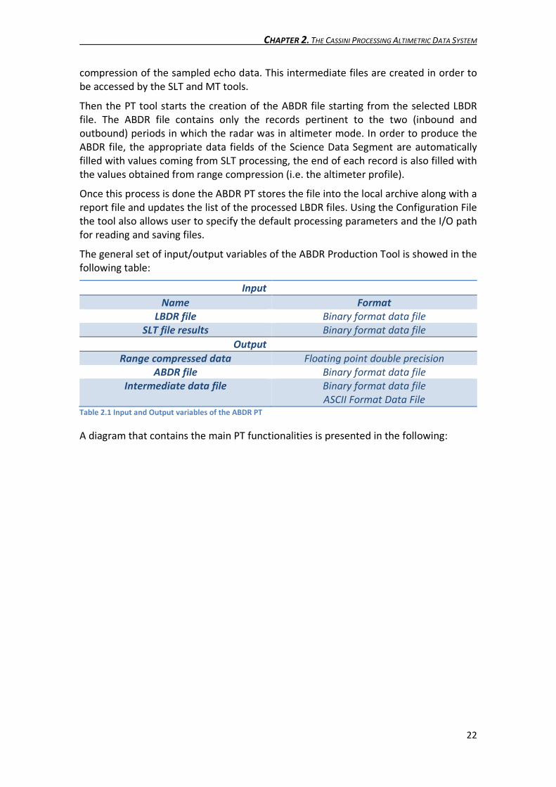
The general set of input/output variables of the ABDR Production Tool is showed in the
following table:
Input
Name Format
LBDR file Binary format data file
SLT file results Binary format data file
Output
Range compressed data Floating point double precision
ABDR file Binary format data file
Intermediate data file Binary format data file
ASCII Format Data File Table 2.1 Input and Output variables of the ABDR PT
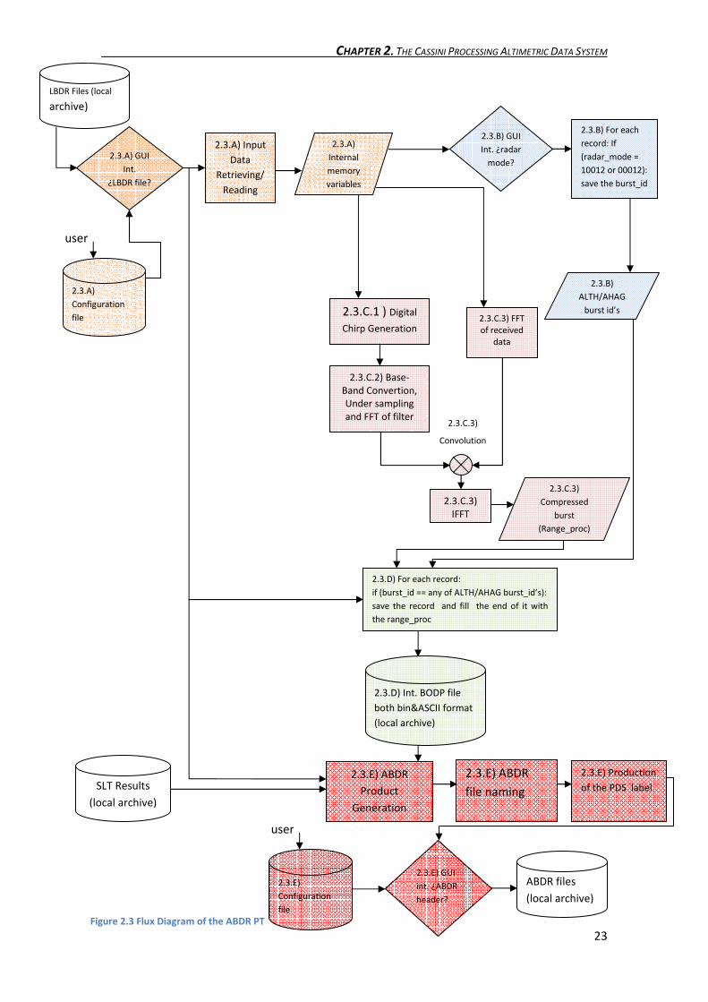
A diagram that contains the main PT functionalities is presented in the following:
CHAPTER 2. THE CASSINI PROCESSING ALTIMETRIC DATA SYSTEM
23
Figure 2.3 Flux Diagram of the ABDR PT
2.3.C.3)
Convolution
2.3.B) For each
record: If
(radar_mode =
10012 or 00012):
save the burst_id
LBDR Files (local
archive)
2.3.A) GUI
Int.
¿LBDR file?
2.3.A)
Internal
memory
variables
2.3.B) GUI
Int. ¿radar
mode?
2.3.A) Input
Data
Retrieving/
Reading
2.3.C.2) Base-
Band Convertion,
Under sampling
and FFT of filter
2.3.C.3) FFT
of received
data
2.3.C.1 ) Digital
Chirp Generation
2.3.B)
ALTH/AHAG
burst id’s
2.3.E) GUI
int. ¿ABDR
header?
ABDR files
(local archive)
2.3.E) ABDR
file naming
2.3.E) Production
of the PDS label SLT Results
(local archive)
2.3.E) ABDR
Product
Generation
2.3.D) Int. BODP file
both bin&ASCII format
(local archive)
2.3.C.3)
Compressed
burst
(Range_proc)
2.3.C.3)
IFFT
2.3.D) For each record:
if (burst_id == any of ALTH/AHAG burst_id’s):
save the record and fill the end of it with
the range_proc
user
2.3.A)
Configuration
file
user
2.3.E)
Configuration
file

CHAPTER 2. THE CASSINI PROCESSING ALTIMETRIC DATA SYSTEM
24
In the following pages will be described the different blocks that need to be
commented with more detail:
2.3.A) Input Data Retrieving/Reading.
Starting from the LBDR file selected by user via GUI, this functionality reads all the data
fields needed and stores them into the local dedicated workstation in order to be
accessed by the following processes. The PT tool allows user to specify the I/O path for
reading and saving files by using the configuration file.
To this end, an external function is used within the main program. Moreover, a C
algorithm is previously used in order to extract and select the compacted data so that
it is possible to create a file, where it will be stored only the data necessary to our
processing and finally to obtain a computational “lightening”.
Once this file is created the data extraction is performed. Since it is used an external
function, it is needed to define those variables to be read and those to be passed:
function [sample_freq, chirp_length, PRI, chirp_start_freq, burst_time,
number_of_pulses, sc_j2000_x, sc_j2000_y, sc_j2000_z,…]=
nomefunction(filename_input, record_start, record_end)
where the variables inside the square brackets are those to be read from the file while
those inside the round brackets are those passed from the main to the function, this is
the input filename, and the first and the last bursts to be processed respectively.
In order to provide these three parameters to the function the main program requests
these variables as input data. To this end, the following windows to introduce such
data have been created:
The figure above figure shows the window used to introduce the record_start and the
record_end, while the following figure shows the window used to select the input file.
Each beam has its own file so it is worth noting that, since the Radar in ALT mode
utilizes the central, nadir-pointing antenna beam, i.e. the beam nº3, the files involving
any of the other beams won’t produce remarkable results:
Figure 2.4 Window to select the input bursts to be processed
CHAPTER 2. THE CASSINI PROCESSING ALTIMETRIC DATA SYSTEM
25
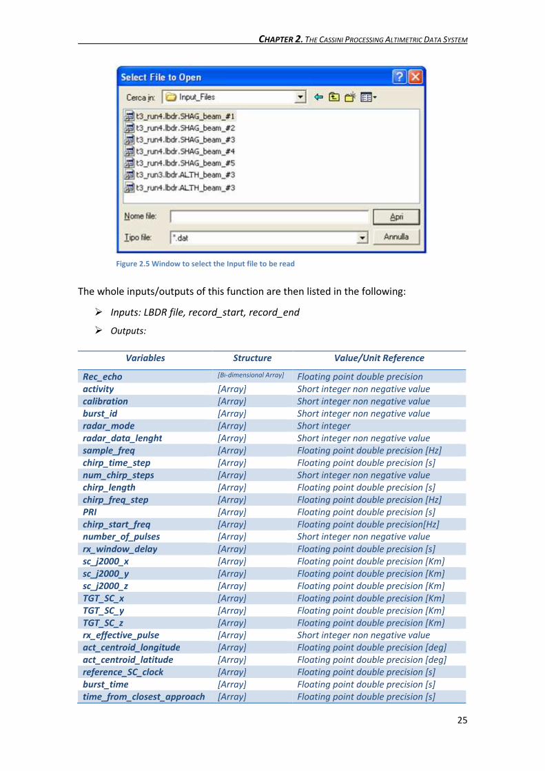
The whole inputs/outputs of this function are then listed in the following:
� Inputs: LBDR file, record_start, record_end
� Outputs:
Variables Structure Value/Unit Reference
Rec_echo [Bi-dimensional Array] Floating point double precision
activity [Array] Short integer non negative value
calibration [Array] Short integer non negative value
burst_id [Array] Short integer non negative value
radar_mode [Array] Short integer
radar_data_lenght [Array] Short integer non negative value
sample_freq [Array] Floating point double precision [Hz]
chirp_time_step [Array] Floating point double precision [s]
num_chirp_steps [Array] Short integer non negative value
chirp_length [Array] Floating point double precision [s]
chirp_freq_step [Array] Floating point double precision [Hz]
PRI [Array] Floating point double precision [s]
chirp_start_freq [Array] Floating point double precision[Hz]
number_of_pulses [Array] Short integer non negative value
rx_window_delay [Array] Floating point double precision [s]
sc_j2000_x [Array] Floating point double precision [Km]
sc_j2000_y [Array] Floating point double precision [Km]
sc_j2000_z [Array] Floating point double precision [Km]
TGT_SC_x [Array] Floating point double precision [Km]
TGT_SC_y [Array] Floating point double precision [Km]
TGT_SC_z [Array] Floating point double precision [Km]
rx_effective_pulse [Array] Short integer non negative value
act_centroid_longitude [Array] Floating point double precision [deg]
act_centroid_latitude [Array] Floating point double precision [deg]
reference_SC_clock [Array] Floating point double precision [s]
burst_time [Array] Floating point double precision [s]
time_from_closest_approach [Array] Floating point double precision [s]
Figure 2.5 Window to select the Input file to be read

CHAPTER 2. THE CASSINI PROCESSING ALTIMETRIC DATA SYSTEM
26
In the following each variable is described with more detail:
• rec_echo: this variable is basically a Bi-dimensional array containing the active
mode time-sampled data as detailed in the previous section. It is used in the
subsequent compression with the matched filter.
• activity: this variable indicates if the present data corresponds to the active
mode operation of the Cassini Radar or not.
• calibration: The following bit patterns are assigned to the various Calibration
Sources: (the three or four character mode name is in parenthesis)
o 0000 = Normal Operation. (norm)
o 0001 = Antenna being used as the Calibration Source. (ant)
o 0010 = Noise Diode being used as the Calibration Source. (diod)
o 0011 = Resistive Load being used as the Calibration Source. (load)
o 0100 = Rerouted Chirp being used as the Calibration Source. (chrp)
o 0101 = Leakage Signal being used as the Calibration Source. (leak)
o 0110 = Radiometer Only Calibration Mode. (rado)
o 0111 = Transmit Only Calibration Mode. (xmto)
o 1000 = Auto-Gain Control. (agc)
o 1001 - 11112 = (reserved by the CTU)
• burst_id: array of short integers, coming from the Engineering Data Segment,
containing the value that uniquely identifies each burst throughout the mission.
minimum_value: 0, maximum_value: 2� -1
• radar_mode: This field represents the radar mode, and is defined as follows:
(the four character mode name is in parenthesis)
o 0000 = ALTL: Altimeter, Low-Resolution (altl)
o 0001 = ALTH: Altimeter, High-Resolution (alth)
o 0010 = SARL: Synthetic Aperture Radar, Low-Resolution (sarl)
o 0011 = SARH: Synthetic Aperture Radar, High-Resolution (sarh)
o 0100 = Radiometer Only (rado)
o 0101 = Inter-Galactic Object (IGO) Calibration (igoc)
o 0110 = Earth Viewing Calibration (evca)
o 0111 = Bi-Static Operation (bsop)
transmit_time_offset [Array] Floating pt.double precision [s]
SC_clock [Array] Floating point double precision
ephemeris_time [Array] Floating point double precision [s]
J2000_sc_vel_x [Array] Floating point double precision [Km]/[s]
J2000_sc_vel_y [Array] Floating point double precision [Km]/[s]
J2000_sc_vel_z [Array] Floating point double precision [Km]/[s]
TGT_sc_vel_x [Array] Floating point double precision [Km]/[s]
TGT_sc_vel_y [Array] Floating point double precision [Km]/[s]
TGT_sc_vel_z [Array] Floating point double precision [Km]/[s]
Incidence_angle [Array] Floating point double precision [deg]
active_geometry_time_offset [Array] Floating point double precision [s]
beam_mask [Array] Short Integer
time_from_epoch [Array] Floating pt.double precision [s] Table 2.2 "Input Data Retrieving/Reading" outputs

CHAPTER 2. THE CASSINI PROCESSING ALTIMETRIC DATA SYSTEM
27
o 1000 = ALTL with Auto Gain (alag)
o 1001 = ALTH with Auto Gain (ahag)
o 1010 = SARL with Auto Gain (slag)
o 1011 = SARH with Auto Gain (shag)
o 1100 � 1111 = (spare)
• radar_data_length: this variable is an array containing the number of valid data
values in the sampled echo data array after decompression, also coming from
the engineering data segment. This number does not have to be constant, and
it will be useful if we would like to know if we can trust a concrete value of the
sampled echo data or not. maximum value: 32000, minimum value: 0
• sample_freq: an array containing the Analog to Digital Converter sampling rate
in Hz. This is the rate at which the echo is sampled. Since Cassini uses video
offset rather than IQ sampling each sample is a real (not complex) value.
possible values: 250 kHz, 1.0 MHz, 2.0 MHz, 10.0 MHz
• chirp_time_step: array containing the duration in time of each single frequency
step. This variable will be needed when we should simulate the transmitted
chirp signal as generated by Cassini DCG in order to perform the matched filter
(section 2.3.C). possible_values: should always be 666.7 ns.
• num_chirp_steps: an array containing the number of chirp steps, this is two
different frequencies before and after the step, thus the number of distinct
frequencies is one more than the number of steps. This variable will be useful
when we should simulate the transmitted chirp signal as generated by Cassini
DCG. minimum_value: 216, maximum_value: 749
• chirp_length: this variable is an array containing the total length of chirp in
seconds. This is equivalent to the width (during transmission) of an individual
pulse. Will also be useful when we should simulate the transmitted chirp signal
as generated by Cassini DCG in order to perform the matched filter.
minimum_value: 0.144 ms, maximum_value: 0.5 ms
• chirp_freq_step: array containing the change in frequency for each chirp step in
Hz. Also useful when we should simulate the transmitted chirp signal as
generated by Cassini DCG. minimum_value: 0 Hz, maximum_value: 117.2 kHz
• PRI: array containing the pulse repetition interval in seconds (the time interval
between successive transmitted (chirped) pulses). Will be used when the
transmitted chirp signal as generated by Cassini DCG is simulated at the Range
Processing Tool. minimum_value: 0.002 ms, maximum_value: 4.092 ms
• chirp_start_freq: array containing the frequency of the first frequency step that
forms the chirp. Useful when we should simulate the transmitted chirp signal as
generated by Cassini DCG in order to perform the matched filter.
minimum_value: 0 Hz maximum_value: 30 MHz
• number_of_pulses: array of integers containing number of pulses transmitted
each burst. Useful when we should simulate the transmitted chirp signal as
generated by Cassini DCG. minimum_value: 0, maximum_value: 255

CHAPTER 2. THE CASSINI PROCESSING ALTIMETRIC DATA SYSTEM
28
• rx_window_delay: array containing the received windows delay, measured
from the beginning of the first pulse in the first PRI to start of receive window.
It includes the PRIs that make up the Transmit Burst and the PRIs between the
end of Transmit Burst and the beginning of the Receive Window. The Receive
Window Delay will always be an integer number of PRIs. minimum_value: 0,
maximum_value: 1023 PRI.
• sc_j2000_x: x- component of S/C position in target_centered J2000 inertial
coordinate system.
• sc_j2000_y: y- component of S/C position in target_centered J2000 inertial
coordinate system.
• sc_j2000_z: z- component of S/C position in target_centered J2000 inertial
coordinate system.
• TGT_SC_x: x- component of S/C position in target body fixed (TBF) coordinate
system.
• TGT_SC_y: y- component of S/C position in target body fixed (TBF) coordinate
system.
• TGT_SC_z: z- component of S/C position in target body fixed (TBF) coordinate
system.
• J2000_sc_vel_x: x- component of S/C velocity vector in the J2000 frame.
• J2000_sc_vel_y: y- component of S/C velocity vector in the J2000 frame.
• J2000_sc_vel_z: z- component of S/C velocity vector in the J2000 frame.
• TGT_sc_vel_x: x- component of S/C velocity vector in the TBF. Value is zero if
target name is none or calibration.
• TGT_sc_vel_y: y- component of S/C velocity vector in the TBF. Value is zero if
target name is none or calibration.
• TGT_sc_vel_z: z- component of S/C velocity vector in the TBF. Value is zero if
target name is none or calibration.
• rx_effective_pulse: array containing the number of pulses which were received
completely within the echo window. Partial pulses are ignored.
• act_centroid_longitud: array containig the longitude of active (two-way)
antenna boresight.
• act_centroid_latitude: array containing the latitude of active (two-way) antenna
boresight.
• reference_SC_clock: Reference spacecraft clock count for each burst. The LSB is
nearly 1 second but not exactly. For exact time references use t_ephem_time.
minimum_value: 0, maximum_value: 2� � 1.
• burst_time: Burst start time expressed as an offset from the reference
spacecraft clock count. The precise spacecraft time at the start of the burst is
reference_SC_clock + burst_time in seconds. minimum_value: 0.0
maximum_value: 1.0

CHAPTER 2. THE CASSINI PROCESSING ALTIMETRIC DATA SYSTEM
29
• t_ephem_time: array that contains the time at start of burst expressed in
seconds since 12:00 AM Jan. 1, 2000. Used for exact time references.
• time_from_closest_approach: t_ephem_time – closest_approach_time.
• transmit_time_offset: array containing the time offset in seconds from
t_ephem_time at which the leading edge of the first transmit pulse leaves the
antenna.
• SC_clock: Encoded spacecraft clock time. This value is used by the SPICE
software employed by the Cassini Navigation Team.
• Incidence_angle: array that contains the angle between the antenna look
direction and the surface normal halfway between transmission and receipt of
the active mode signal.
• active_geometry_time_offset: array that contains the time offset in seconds
from burst reference time (t_ephem_time) for which the active geometry fields
were computed. Active mode geometry is computed for the time halfway
between the midpoint of the transmission and the midpoint of the active mode
receiver window. The full set of measurement geometry for each case includes:
the polarization orientation angle, emission/incidence angle, azimuth angle, the
measurement centroid, and four points on the 3 dB gain contour of the
measurement.
• beam_mask: since the Cassini Radar is a multimode instrument with up to 5
different beams, a beam mask is needed in order to be able to activate de
different beams depending on the radar mode. This variable is an array
containing the following bit patterns describing the possible Beam Masks used
by the Cassini RADAR DSS, minimum_value: 0, maximum_value: 31:
o 00000 = All beams disabled (Used during internal source Calibration
modes such as noise diode, resistive load and rerouted chirp).
o 00001 = Beam #1 Only enabled.
o 00010 = Beam #2 Only enabled.
o 00011 = Beams #2 and #1 enabled.
o 10000 = Beam #5 Only enabled.
o 11010 = Beams #5, #4 and #2 enabled.
o 11111 = All Five Beams enabled.
• time_from_epoch: t_ephem_time – epoch_time. The value of epoch_time is
usually the same as the closest approach time but may differ occasionally for
logistic reasons.
*two coordinate frames are used to compute spacecraft ephemeris and attitude
information: An inertial frame (J2000) centered on the target (typically Titan), and the
target body fixed frame (TBF). Although both frames are centered on the target, the
orientation of the frames differs. The TBF frame maintains a constant orientation with
respect to any point on the surface of the target. For example, if the target were Earth,
the TBF coordinates of the point 100 m above the Washington monument would not
change with time. The inertial frame coordinate system is the standard J2000
coordinate system translated so that it is centered at the target’s (Titan’s) center at the

CHAPTER 2. THE CASSINI PROCESSING ALTIMETRIC DATA SYSTEM
30
time of the start of the burst. With these variables we will be able to calculate the
distance from the spacecraft to the center of Titan, for each burst.
2.3.B) Radar Mode Reading.
Starting from the variables: radar_mode, and burst_id, from the engineering data
segment, this function stores into the local dedicated workstation all burst_id’s from
those records in which the radar was in altimeter mode:
• radar_mode = 00012 � Altimeter, High Resolution, ALTH.
• radar_mode = 10012 � Altimeter with Auto Gain, AHAG.
depending on previous user selection via GUI. So if radar mode is one of this two the
burst_id will be stored in the output of this function.
The whole inputs/outputs of this function are listed in the following:
� Inputs: radar_mode, burst_id
� Outputs: ALTH/AHAG burst id’s
2.3.C) Range Processing.
In this section is explained how the received signal is processed in order to achieve an
optimal signal waveform that should be taken by the Science Look Tool, to estimate
Titan’s surface’s significant parameters in the most efficient way. A complete
description of the Physical concepts of the range processing can be found in 3.1
section.
As detailed on 3.1 the filter that maximizes the SNR (matched filter) is actually the
conjugate of signal itself inverted, and the transmitted signal waveform that yields the
best distance resolution is the chirp. So in order to perform the matched filtering it is
needed to simulate the chirp signal as that generated by Cassini DCG.
To this end the chirp is generated at 30MHz and then the Doppler frequency is
subtracted see section 3.6, the resulting signal is undersampled at 10MHz. The
matched filter is done in frequency domain by implementing the FFT of both simulated
chirp and received data and by doing the convolution of both signals. In the resulting
signal all the energy is gathered into a narrow peak in the compressed pulse
The full detailed algorithm is here below reported in terms of pseudocode:
1. fc=5*1e6; 2. Np_samples = floor(PRI.*sample_freq/2); 3. t_start = chirp_start_freq./rate_chirp; 4. t_stop = (chirp_start_freq+B)./rate_chirp; 5. for kk=record_start:record_end 6. td=t_start:1/FC:t_stop; 7. t=0:1/FC:length(td)/FC-1/FC; 8. fd=rate_chirp*td; 9. fased=cumsum(fd)*1/FC*2*pi+rate_chirp*t_start*t_start*pi;
2.3.C.1 Digital Chirp Generation
CHAPTER 2. THE CASSINI PROCESSING ALTIMETRIC DATA SYSTEM
31
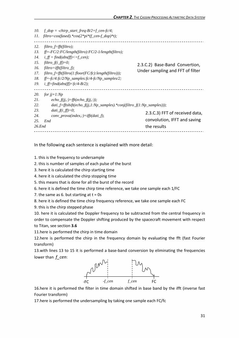
10. f_dop = -chirp_start_freq-B/2+f_cen-fc/4; 11. filtro=cos(fased).*cos(2*pi*(f_cen-f_dop)*t); 12. filtro_f=fft(filtro); 13. ff=-FC/2:FC/length(filtro):FC/2-1/length(filtro); 14. i_ff = find(abs(ff)<=f_cen); 15. filtro_f(i_ff)=0; 16. filtro=ifft(filtro_f); 17. filtro_f=fft(filtro(1:floor(FC/fc):length(filtro))); 18. ff=-fc/4:fc/2/Np_samples:fc/4-fc/Np_samples/2; 19. i_ff=find(abs(ff)<fc/4-B/2); 20. for jj=1:Np 21. echo_f(jj,:)=fft(echo_f(jj,:)); 22. dati_f=fftshift(echo_f(jj,1:Np_samples).*conj(filtro_f(1:Np_samples))); 23. dati_f(i_ff)=0; 24. conv_prova(index,:)=ifft(dati_f); 25. End 26.End
In the following each sentence is explained with more detail:
1. this is the frequency to undersample
2. this is number of samples of each pulse of the burst
3. here it is calculated the chirp starting time
4. here it is calculated the chirp stopping time
5. this means that is done for all the burst of the record
6. here it is defined the time chirp time reference, we take one sample each 1/FC
7. the same as 6. but starting at t = 0s
8. here it is defined the time chirp frequency reference, we take one sample each FC
9. this is the chirp stepped phase
10. here it is calculated the Doppler frequency to be subtracted from the central frequency in
order to compensate the Doppler shifting produced by the spacecraft movement with respect
to Titan, see section 3.6
11.here is performed the chirp in time domain
12.here is performed the chirp in the frequency domain by evaluating the fft (fast Fourier
transform)
13.with lines 13 to 15 it is performed a base-band conversion by eliminating the frequencies
lower than f_cen:
16.here it is performed the filter in time domain shifted in base band by the ifft (inverse fast
Fourier transform)
17.here is performed the undersampling by taking one sample each FC/fc
FC -FC -f_cen f_cen
2.3.C.2) Base-Band Convertion,
Under sampling and FFT of filter
2.3.C.3) FFT of received data,
convolution, IFFT and saving
the results

CHAPTER 2. THE CASSINI PROCESSING ALTIMETRIC DATA SYSTEM
32
18.with lines 18, 19 and 23 it is performed out-band samples elimination following the same
procedure of the base-band conversion
20. this means that this is done for each burst pulse
21.here it is evaluated the fft of the jj_th pulse of the burst of the received echo data
22.here it is performed the convolution of the fft of the jj_th pulse with the matched filter, this
is the conjugated of 17.
24.finally it is performed the ifft of 22 in order to obtain and save the range compressed data
The whole inputs/outputs of this function are listed in the following:
� Inputs: PRI, sample_freq, chirp_start_freq, number_of_pulses, rec_echo, B,
rate_chirp and FC.
� Output: range_proc
2.3.D) Intermediate files generation
In order to be accessed by the SLT and the MT for internal data processing, this tool
generates the intermediate BODP files by saving the data records pertinent to
ALTH/AHAG radar operational modes and by filling the end of each record with the
range compressed data (range_proc). The final file is saved into the local archive.
In order to achieve it, this tool looks the burst_id of each record of the input LBDR file
and saves only those records that match with those in the ALTH/AHAG burst id’s
stored by the radar mode reading tool.
The whole inputs/outputs of this function are listed in the following:
� Inputs: range_proc, input LBDR file, and ALTH/AHAG burst id’s
� Outputs: Intermediate BODP data files in both binary and ASCII formats.
2.3.E) ABDR file generation, file naming, labeling and saving
Starting from the LBDR selected file and taking into account only the two periods in
which the radar was in altimeter mode, this tool fills the end of each record with the
range compressed data from the Intermediate BODP file (i.e. altimeter profile). In
addition the appropriate data fields in the Science Data Segment are filled with the
values obtained from the SLT processing:
• range_to_target: distance from the satellite radar to the observed surface.
• rtt_std: estimated standard deviation of the residual error in the
range_to_target measurement.
• altimeter_profile_range_start: a floating point double precision containing the
range of the first altimeter profile value in each pulse.
• altimeter_profile_range_step: a floating point double precision containing the
difference in range between consecutive range bins in altimeter profile.
• altimeter_profile_length: this is an integer containing the number of valid
entries in altimeter profile.
CHAPTER 2. THE CASSINI PROCESSING ALTIMETRIC DATA SYSTEM
33
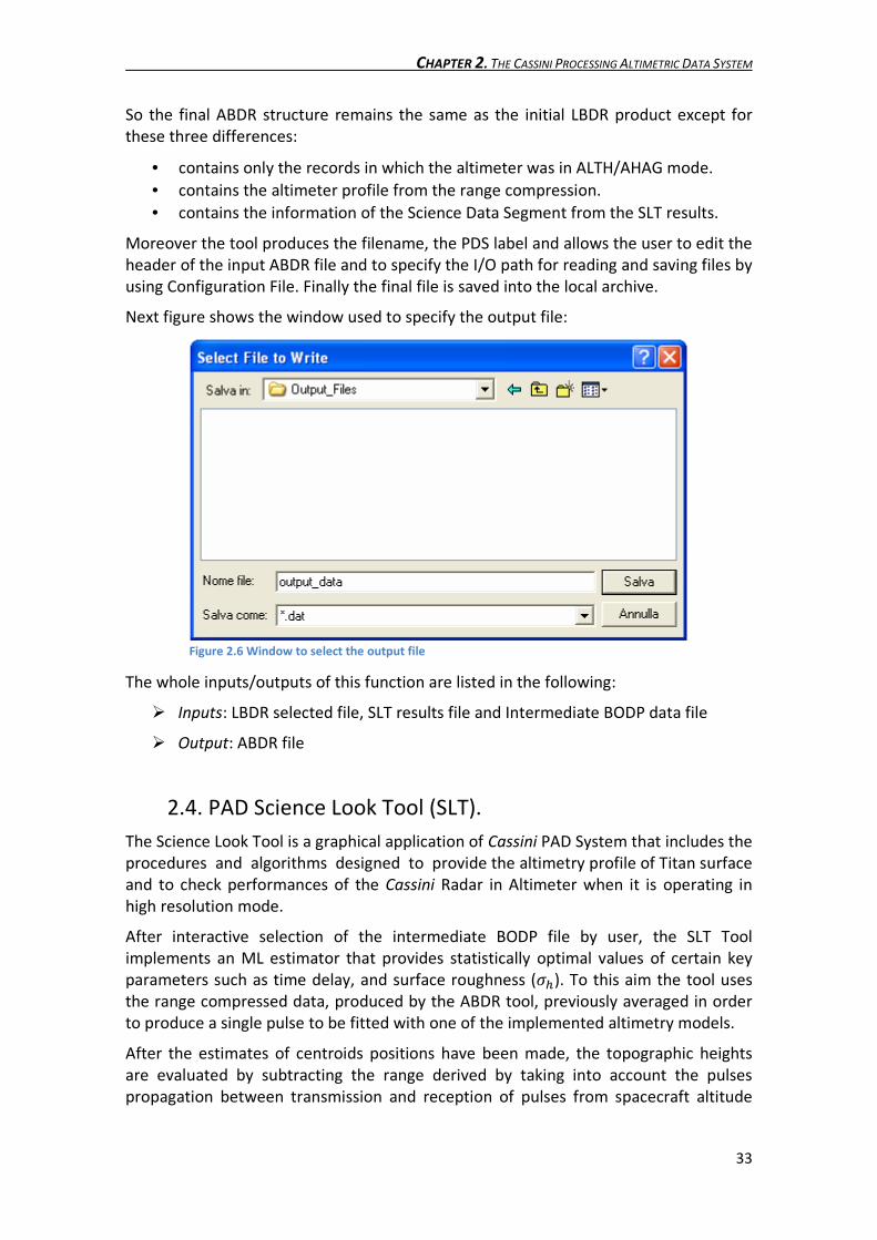
So the final ABDR structure remains the same as the initial LBDR product except for
these three differences:
• contains only the records in which the altimeter was in ALTH/AHAG mode.
• contains the altimeter profile from the range compression.
• contains the information of the Science Data Segment from the SLT results.
Moreover the tool produces the filename, the PDS label and allows the user to edit the
header of the input ABDR file and to specify the I/O path for reading and saving files by
using Configuration File. Finally the final file is saved into the local archive.
Next figure shows the window used to specify the output file:
The whole inputs/outputs of this function are listed in the following:
� Inputs: LBDR selected file, SLT results file and Intermediate BODP data file
� Output: ABDR file
2.4. PAD Science Look Tool (SLT).
The Science Look Tool is a graphical application of Cassini PAD System that includes the
procedures and algorithms designed to provide the altimetry profile of Titan surface
and to check performances of the Cassini Radar in Altimeter when it is operating in
high resolution mode.
After interactive selection of the intermediate BODP file by user, the SLT Tool
implements an ML estimator that provides statistically optimal values of certain key
parameters such as time delay, and surface roughness (��). To this aim the tool uses
the range compressed data, produced by the ABDR tool, previously averaged in order
to produce a single pulse to be fitted with one of the implemented altimetry models.
After the estimates of centroids positions have been made, the topographic heights
are evaluated by subtracting the range derived by taking into account the pulses
propagation between transmission and reception of pulses from spacecraft altitude
Figure 2.6 Window to select the output file

CHAPTER 2. THE CASSINI PROCESSING ALTIMETRIC DATA SYSTEM
34
with respect to the surface (i.e. orbital range-Titan mean radius) satellite orbital range
to target.
Moreover, the tool allows the simulation of the performances and the waveform
analysis of the Cassini Radar Altimeter. The SLT intermediate files and results are
stored into the local dedicated workstation where procedure is running, or into the
local archive if data shall be shared with other tools.
The SLT results are used subsequently by the ABDR Production Tool to generate the
ABDR file. The SLT also generates automatically a text file containing all relevant
information on SLT processing outputs and plots of main results, to be stored into the
local archive in order to be submitted to the scientific community for further validation
of data.
Users may export (i.e. print/save) Plot files containing results produced by SLT, e.g.
relevant processing parameters, MLE procedure results, relative elevations of Titan’s
surface vs. along-track distance (i.e. topographic profiles), altimeter waveforms vs.
range bins, ancillary data (e.g. observation geometry and orbital parameters vs. time,
instrument data, etc.), surface parameters vs. along-track distance, etc.
The general set of Input/Output Variables of SLT Tool is reported in the following table:
Input
Name Format
Intermediate data file Binary format data file
ASCII Format Data File
Output
SLT file results Binary format data file
Table 2.3 Input and Output variables of the SLT
SLT Results files are automatically produced for both ALTH/AHAG operating modes. In
particular, the SLT Results files contain:
• Real/Simulated IR: the real impulse response is that calculated by averaging the
range compressed data coming from the intermediate BODP file. The simulated
Impulse Response obtained by implementing the models described in 3.3
section
• Pulse Centroid Position estimate: the value of the centroid position obtained by
the MLE algorithm explained in the 2.4.D section
• Titan Surface Roughness estimate: the value of the titan surface roughness ����. • Surface slope: the value of the surface slope obtained by computing the
derivative of the estimated heights

CHAPTER 2. THE CASSINI PROCESSING ALTIMETRIC DATA SYSTEM
35
• Topographic profile: the final altitudes computed from values obtained with the
MLE algorithm
• Range to target: the final estimated distance from the spacecraft to the Titan’s
surface
• rtt_std: estimated standard deviation of the residual error in the range to
target measurement
• Altimeter profile range start
• Altimeter profile range step
• Altimeter profile length
A diagram that contains the main PT functionalities is presented in the following:
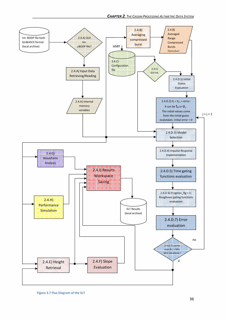
CHAPTER 2. THE CASSINI PROCESSING ALTIMETRIC DATA SYSTEM
36
si
user
2.4.E) Height
Retrieval
2.4.F) Slope
Evaluation
2.4.I) Results
Workspace
Saving
SLT Results
(local archive)
2.4.D.2) Xj = Xj-1 + error:
X can be t0 or σs .
The initial values come
from the initial guess
evalutaion, initial error = 0
2.4.D.3) Model
Selection
2.4.D.7) Error
evaluation
2.4.D.7) ¿error
<eps & j > Min.
MLE iterations?
j = j + 1
no
2.4.H)
Performance
Simulation
Int. BODP file both
bin&ASCII format
(local archive)
2.4.B)
Averaging
compressed
burst
2.4.C)
GUI Int.
2.4.D.1) Initial
Guess
Evaluation
2.4.G)
Waveform
Analysis
2.4.A) GUI
Int.
¿BODP file?
2.4.A) Internal
memory
variables
2.4.A) Input Data
Retrieving/Reading
2.4.B)
Averaged
Range
Compressed
Bursts
(impulse)
2.4.D.4) Impulse Response
implementation
2.4.D.5) Time gating
functions evaluation
2.4.D.6) If sigmas_flg = 1:
Roughness gating functions
evaluation
2.4.C)
Configuration
file
Figure 2.7 Flux Diagram of the SLT

CHAPTER 2. THE CASSINI PROCESSING ALTIMETRIC DATA SYSTEM
37
In the following pages will be described the different blocks that need to be
commented with more detail:
2.4.A) Input Data Retrieving/Reading
Starting from the intermediate BODP file, produced by the ABDR PT and selected by
user, this functionality reads all the data fields and stores them into the local dedicated
workstation. The procedure is similar to that of the section 2.3.A.
The whole inputs/outputs of this function are listed in the following:
� Input: Intermediate BODP’s data files in both binary and ASCII formats.
� Outputs: Internal memory variables (table 2.2)
2.4.B) Averaging compressed burst
The � compressed pulses within the burst are averaged so that each compressed
burst becomes an array given by only one averaged pulse-compressed echo. The
averaged range compressed burst is stored in an internal memory bi-dimensional
array.
The whole inputs/outputs of this function are listed in the following:
� Input: range_proc: bidimensional array of floating point double precision
containing range compressed burst.
� Output: data: an array containing averaged range compressed burst.
The process is performed in the following way:
The acquired samples � � ���, … , ���, due to the multiplicity of the scattering
elements (each acquired sampled is considered as the sum of the contribution of
multiple scattering elements), may be approximated, taking into account the central
limit theorem, as two complex Gaussian distributed variables: �� � � � !"�, and so, as
it is commonly known if we calculate:
|��| � $ � � "� �2.4. B. 1�
the resulting process has a Rayleigh distribution. Now if we do |��| � )� , since the
radar echo is typically processed after square law detection we obtain, as it is also
known, an Exponential distributed process, with mean equal to the i-th sample of the
radar averaged impulse response evaluated by using equations 2.4.D.4.2, 2.4.D.4.3 or
2.4.D.4.4 that will be detailed in the following sections.

CHAPTER 2. THE CASSINI PROCESSING ALTIMETRIC DATA SYSTEM
38
The burst is
segmented
into � pulses
Each burst of N samples contains � pulses (typically 15 for the high resolution
altimeter mode) that can be used to obtain a unique single pulse by performing an
incoherent summation. This operation that reduces the speckled noise is done in the
following way:
) � �)�, … , )�� *��/�,-...../ )�,0* �12324 )� � )�, … , )* ) � )*5�, … , ) * 6 6 ) �, � )��,7��*5�, … , )�
8 �2.4. B. 2� )9:;< � 1� )=*5> ?@A 1 B ; B � �2.4. B. 3��,7�
=��
As a result of this, the )9� averaged sample can be approximately viewed as Gaussian
distributed, with: DE)9�F � DE)�F � G�� �2.4. B. 4� HI�E)9�F � HI�E)�F� � G�� � �2.4. B. 5�
In this way, since the average is performed in an incoherent way, the speckle that is
overlapping to received echoes is reduced in a significant way.
approximately
Gaussian
distributed: )9:;< Exponential
distributed samples: ) � �)�, … , )��
complex
Gaussian
samples: �� � � � !"�video offset
baseband
Matched
Filter $ � � "�
Rayleigh
distributed
samples
| |
Digital Chirp generation
from PAD sytem,
section 2.3.C
Incoherent
averaging
Figure 2.8 Block diagram of the process of the received echo signal in the Cassini PAD System

CHAPTER 2. THE CASSINI PROCESSING ALTIMETRIC DATA SYSTEM
39
The result of the averaging process is showed in the next figure:
2.4.C) Configuration file
The SLT tool allows user to specify the default processing parameters by using the
Configuration file. In particular the Configuration file will contain:
• Threshold value for off-Nadir angles: the values of the pointing angle on
which the MLE estimator is based to switch among the different fitting
models.
• Minimum number of MLE iterations: the value of the minimum iterations
that the algorithm should perform before stopping
• Method for centroid initial value evaluation: the method selected to
evaluate the initial values of the time delay
• Sigmas_flg: the flag used to indicate if the surface roughness estimation
must be performed or not
All these parameters will be described in detail in the corresponding paragraphs.
2.4.D) Surface Parameters Estimation
This tool of the SLT provides statistically optimal estimates of the Titan’s surface’s
significant parameters such as time delay (K�) and roughness (��).
Figure 2.9 Averaged pulse produced for each burst
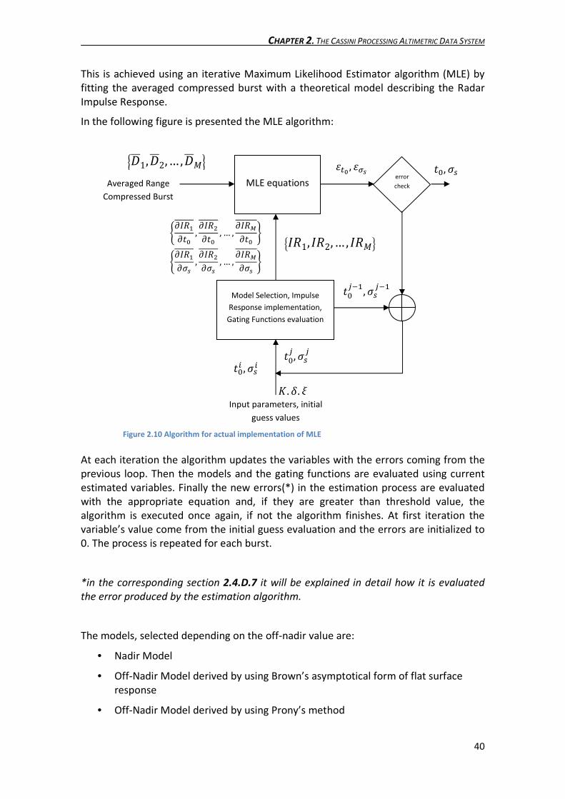
CHAPTER 2. THE CASSINI PROCESSING ALTIMETRIC DATA SYSTEM
40
This is achieved using an iterative Maximum Likelihood Estimator algorithm (MLE) by
fitting the averaged compressed burst with a theoretical model describing the Radar
Impulse Response.
In the following figure is presented the MLE algorithm:
At each iteration the algorithm updates the variables with the errors coming from the
previous loop. Then the models and the gating functions are evaluated using current
estimated variables. Finally the new errors(*) in the estimation process are evaluated
with the appropriate equation and, if they are greater than threshold value, the
algorithm is executed once again, if not the algorithm finishes. At first iteration the
variable’s value come from the initial guess evaluation and the errors are initialized to
0. The process is repeated for each burst.
*in the corresponding section 2.4.D.7 it will be explained in detail how it is evaluated
the error produced by the estimation algorithm.
The models, selected depending on the off-nadir value are:
• Nadir Model
• Off-Nadir Model derived by using Brown’s asymptotical form of flat surface
response
• Off-Nadir Model derived by using Prony’s method
LMG��MK� , MG� MK� , … , MG�*MK� N
LMG��M�� , MG� M�� , … , MG�*M�� N
K�, �� OPQ , ORS
K�=7�, ��=7�
K�= , ��=
T, U, V
Averaged Range
Compressed Burst
Input parameters, initial
guess values
MLE equations
Model Selection, Impulse
Response implementation,
Gating Functions evaluation
error
check
K�� , ���
W)1,)2,… ,)�X
YG�1, G�2,… , G��Z
Figure 2.10 Algorithm for actual implementation of MLE
method
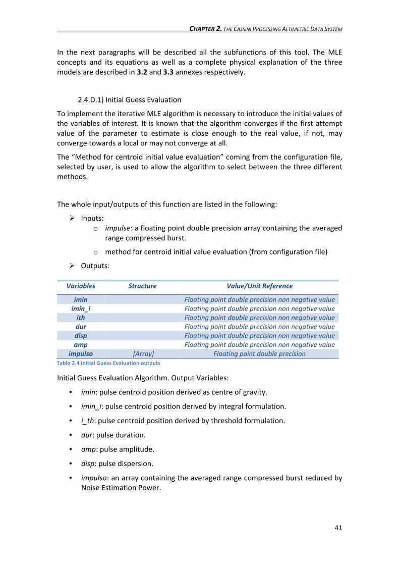
CHAPTER 2. THE CASSINI PROCESSING ALTIMETRIC DATA SYSTEM
41
In the next paragraphs will be described all the subfunctions of this tool. The MLE
concepts and its equations as well as a complete physical explanation of the three
models are described in 3.2 and 3.3 annexes respectively.
2.4.D.1) Initial Guess Evaluation
To implement the iterative MLE algorithm is necessary to introduce the initial values of
the variables of interest. It is known that the algorithm converges if the first attempt
value of the parameter to estimate is close enough to the real value, if not, may
converge towards a local or may not converge at all.
The “Method for centroid initial value evaluation” coming from the configuration file,
selected by user, is used to allow the algorithm to select between the three different
methods.
The whole input/outputs of this function are listed in the following:
� Inputs:
o impulse: a floating point double precision array containing the averaged
range compressed burst.
o method for centroid initial value evaluation (from configuration file)
� Outputs:
Initial Guess Evaluation Algorithm. Output Variables:
• imin: pulse centroid position derived as centre of gravity.
• imin_i: pulse centroid position derived by integral formulation.
• i_th: pulse centroid position derived by threshold formulation.
• dur: pulse duration.
• amp: pulse amplitude.
• disp: pulse dispersion.
• impulso: an array containing the averaged range compressed burst reduced by
Noise Estimation Power.
Variables Structure Value/Unit Reference
imin Floating point double precision non negative value
imin_i Floating point double precision non negative value
ith Floating point double precision non negative value
dur Floating point double precision non negative value
disp Floating point double precision non negative value
amp Floating point double precision non negative value
impulso [Array] Floating point double precision
Table 2.4 Initial Guess Evaluation outputs

CHAPTER 2. THE CASSINI PROCESSING ALTIMETRIC DATA SYSTEM
42
The algorithm that provides the initial values of the estimation is described in the
following:
In order to obtain the order of magnitude of the variance in the estimate of the COG
position, these subsequent steps have been followed:
• burst #14364 from Ta fly-by has been selected
• simulated waveform has been obtained by adding a white Gaussian thermal
noise to the model, see figure 2.12
• the average of the 15 pulses within the burst has been performed in order to
reduce the noise in individual pulses
• the ML estimator has been run N times, see figure 2.13
• the variance (in pixels) of the N estimates of the centroid position has been
evaluated.
2.4.D.1) Initial
Guess
Evaluation
Pulse centre
of gravity
Integral
formulation
Leading
Edge detection
• Configuration
file
• Impulse
Method
for
Centroid?
�[: ] ^�_ �� B �̀� ��aba9��� ^c_ �� d �̀��aea9
=�� ] � fg;
^�_ and ^c_ �left and right side of pulse’s power.
So the centroid position is considered the point where de
difference between both sides of the pulse’s power is
minimum.
K̂� � ij^�j�kji^�j�kj
the centre of gravity (COG), related to the time
delay of the average surface:
where ^�j� is the received echo waveform
lm � �i^�j�kj�knP , knP � �i^�j�kj� i^ �j�kj , om � �ij ^�j�kji^�j�kj � K̂�
Initial Centroid position is obtained using leading edge
detection by mean of a threshold, to evaluate this threshold the
following variables are evaluated:
• Pulse amplitude: lm , related to the surface reflectivity
• Pulse duration: knP , related to the surface roughness
• Dispersion: om , which allows the discrimination between two
close echoes
Where ^�j�is the recieved echo waveform
Figure 2.11 Algorithm for actual evaluation of initial guess evaluation

CHAPTER 2. THE CASSINI PROCESSING ALTIMETRIC DATA SYSTEM
43
2
2.4.D.3) Model Selection
The best theoretical model to use is selected by reading the off-nadir angle value.
Starting from experimental results, threshold values are defined for off-Nadir angle. If
the off-Nadir value is between the specified intervals, the algorithm will be able to
select one model to fit in the Cassini data rather than the others.
In the following will be described the procedure followed to determine the threshold
values of each model depending on the mean integral relative error (MIRE), which has
Figure 2.12 Fitting between simulated and real echo waveforms (ξ=0.23°, h =5500 km)
Figure 2.13 Estimations of COG position over N=100 runs (burst # 14364)
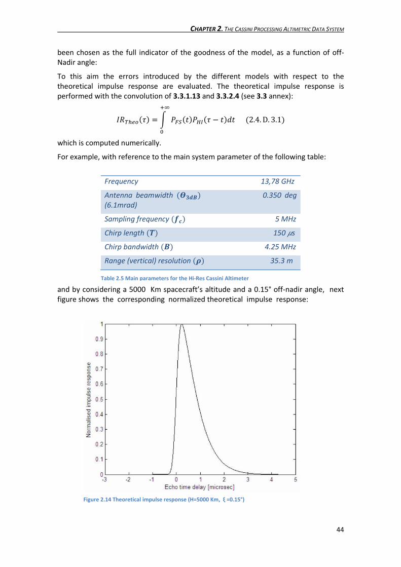
CHAPTER 2. THE CASSINI PROCESSING ALTIMETRIC DATA SYSTEM
44
been chosen as the full indicator of the goodness of the model, as a function of off-
Nadir angle:
To this aim the errors introduced by the different models with respect to the
theoretical impulse response are evaluated. The theoretical impulse response is
performed with the convolution of 3.3.1.13 and 3.3.2.4 (see 3.3 annex):
G�p�qr�j� � s tuv�K�twx�j � K�kK5y� �2.4. D. 3.1�
which is computed numerically.
For example, with reference to the main system parameter of the following table:
and by considering a 5000 Km spacecraft’s altitude and a 0.15° off-nadir angle, next
figure shows the corresponding normalized theoretical impulse response:
Frequency 13,78 GHz
Antenna beamwidth �{|}~� 0.350 deg
(6.1mrad)
Sampling frequency ���� 5 MHz
Chirp length ��� 150 �s
Chirp bandwidth �~� 4.25 MHz
Range (vertical) resolution ��� 35.3 m
Table 2.5 Main parameters for the Hi-Res Cassini Altimeter
Figure 2.14 Theoretical impulse response (H=5000 Km, ξ =0.15°)
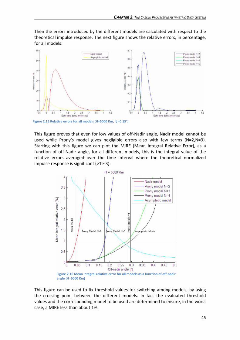
CHAPTER 2. THE CASSINI PROCESSING ALTIMETRIC DATA SYSTEM
45
Then the errors introduced by the different models are calculated with respect to the
theoretical impulse response. The next figure shows the relative errors, in percentage,
for all models:
This figure proves that even for low values of off-Nadir angle, Nadir model cannot be
used while Prony’s model gives negligible errors also with few terms (N=2,N=3).
Starting with this figure we can plot the MIRE (Mean Integral Relative Error), as a
function of off-Nadir angle, for all different models, this is the integral value of the
relative errors averaged over the time interval where the theoretical normalized
impulse response is significant (>1e-3):
This figure can be used to fix threshold values for switching among models, by using
the crossing point between the different models. In fact the evaluated threshold
values and the corresponding model to be used are determined to ensure, in the worst
case, a MIRE less than about 1%.
Figure 2.15 Relative errors for all models (H=5000 Km, ξ =0.15°)
Figure 2.16 Mean integral relative error for all models as a function of off-nadir
angle (H=6000 Km)

CHAPTER 2. THE CASSINI PROCESSING ALTIMETRIC DATA SYSTEM
46
The final selected threshold values are listed in the following table:
Threshold off-nadir angle [deg] Model to be used � � � �0.04 Nadir �. �� B � �0.16 Prony’s N=2 �. �� B � �0.26 Prony’s N=3 �. �� B � �0.29 Prony’s N=4 � d �. �� Asymptotic Table 2.6 Threshold values for off-nadir angle and corresponding model for assuring a MIRE < 1 %
Finally it is worth nothing that error’s models (MIRE in this case) are almost
independent of spacecraft altitude, at least in the Cassini altimeter operative range as
it shows the next figures:
Figure 2.17 Mean integral relative error for Nadir and Asymptotic models as a
function of spacecraft altitude ( ξ =0.15°)
Figure 2.18 Mean integral relative error for Prony’s model as a function of
spacecraft altitude ( ξ =0.15°)
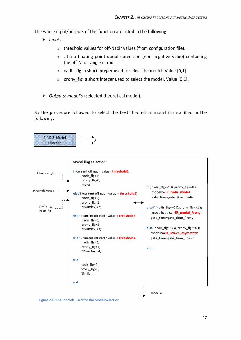
CHAPTER 2. THE CASSINI PROCESSING ALTIMETRIC DATA SYSTEM
47
The whole input/outputs of this function are listed in the following:
� Inputs:
o threshold values for off-Nadir values (from configuration file).
o zita: a floating point double precision (non negative value) containing
the off-Nadir angle in rad.
o nadir_flg: a short integer used to select the model. Value [0,1].
o prony_flg: a short integer used to select the model. Value [0,1].
� Outputs: modello (selected theoretical model).
So the procedure followed to select the best theoretical model is described in the
following:
Model flag selection:
if (current off nadir value <threshold1)
nadir_flg=1;
prony_flg=0;
NN=0;
elseif (current off nadir value < threshold2)
nadir_flg=0;
prony_flg=1;
NN(index)=2;
elseif (current off nadir value < threshold3)
nadir_flg=0;
prony_flg=1;
NN(index)=3;
elseif (current off nadir value < threshold4)
nadir_flg=0;
prony_flg=1;
NN(index)=4;
else
nadir_flg=0;
prony_flg=0;
NN=0;
end
modello
2.4.D.3) Model
Selection
if ( nadir_flg==1 & prony_flg==0 )
modello=IR_nadir_model
gate_time=gate_time_nadir
elseif (nadir_flg==0 & prony_flg==1 );
[modello aa cc]=IR_model_Prony
gate_time=gate_time_Prony
else (nadir_flg==0 & prony_flg==0 );
modello=IR_Brown_asymptotic
gate_time=gate_time_Brown
end
threshold vaues
off-Nadir angle
prony_flg
nadir_flg
Figure 2.19 Pseudocode used for the Model Selection
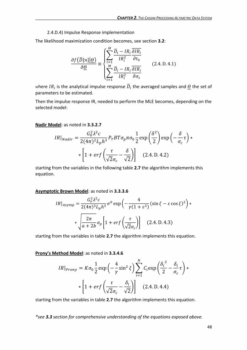
CHAPTER 2. THE CASSINI PROCESSING ALTIMETRIC DATA SYSTEM
48
2.4.D.4) Impulse Response implementation
The likelihood maximization condition becomes, see section 3.2:
M?�)9:;<���M� �12324)9� � G��G�� MG��MK�
*���)9� � G��G�� MG��M��*���
8 �2.4. D. 4.1� Where G�� is the analytical impulse response )9� the averaged samples and � the set of
parameters to be estimated.
Then the impulse response IR, needed to perform the MLE becomes, depending on the
selected model:
Nadir Model: as noted in 3.3.2.7 8G�|��c�� � �� � �2�4�� ���� tp������� 12 exp �U 2 exp ¡� U�¢ j£ ¤
¤ ¥1 � ¦A? � j√2�¢ � U√2 ¨ �2.4. D. 4.2� starting from the variables in the following table 2.7 the algorithm implements this
equation.
Asymptotic Brown Model: as noted in 3.3.3.6 8G�|©�ª«� � �r � �2�4������� �� exp ¡� 4¬�1 � O � �sin V � O cos V� £ ¤
¤ � 2�l � 2² �� ¥1 � ¦A? � j√2�¢ ¨ �2.4. D. 4.3�
starting from the variables in table 2.7 the algorithm implements this equation.
Prony’s Method Model: as noted in 3.3.4.6
8G�|³�r>ª � T�� 12 exp ¡�4¬ sin V£ �́exp �U� 2 � U��¢ j ¤����
¤ ¥1 � ¦A? � j√2�¢ � U�√2 ¨ �2.4. D. 4.4� starting from the variables in table 2.7 the algorithm implements this equation.
*see 3.3 section for comprehensive understanding of the equations exposed above.

CHAPTER 2. THE CASSINI PROCESSING ALTIMETRIC DATA SYSTEM
49
The whole inputs/output of this subfunction are listed in the following:
� Inputs:
Variables Structure Value/Unit Reference
t [Array] Floating point double precision [s]
t0 Floating point double precision [s]
H Floating point double precision. Non negative value [m]
Radius Short integer. Non negative value [m]
sigma_h [m]
sigma_p Floating point double precision. Constant value [m]
gamma Floating point double precision. Adimensional Constant
c Floating point double precision. Constant value [m]/[s]
zita Floating point double precision. Non negative value[rad]
B Floating point double precision [Hz]
sigma_c Floating point double precision [s]
NN Short Integer Min: 1;Max:4
Table 2.7 Inputs of the Impulse Response Implementation.
In the following each variable will be described with more detail:
• t: an array containig the time reference, needed when we need to implement
the impulse response since j � K � K� � K � 2�/�.
• K�: Time Delay for propagation Radar-Target-Radar.
• H: this value is the Satellite Range to Target.
• Radius: The Titan Mean equatorial radius.
• sigma_h: In this variable will be stored the value of Titan’s surface roughness: �� � ��/2���.
• sigma_p: Parameter related to point target 3 dB width. It is needed when we
need to implement the impulse response, since �¢ � �� � �� . Typically �� � �/√8 ln 2.
• gamma: Parameter related to point target 3dB width. Referred as ¬ in 3.3
section �¬ � �2 sin ���c�/2� / ln�0.5��. As can be seen in table 2.5: ��c� � 0.350 deg �6.1mrad�. • c: speed of light.
• zita: This variable stores the value of the off-nadir angle, it is necessary in order
to implement the impulse response. Referred as ξ in 3.3 section.
• B: Chirp band, needed to implement the impulse response.
• sigma_c: Total spreading of the average echo. This value is needed in order to
implement the impulse response.
• NN: Index of Prony’s approximation order, also needed in order to implement
the impulse response, minimum_value: 1, maximum_value: 4.

CHAPTER 2. THE CASSINI PROCESSING ALTIMETRIC DATA SYSTEM
50
� Outputs:
Variables Structure Value/Unit reference
IR_nadir [Array] Floating point double precision
IR_Brown [Array] Floating point double precision
PFS_Brown_approx [Array] Floating point double precision
IR [Array] Floating point double precision
aa [Array] Complex Double Precision
cc [Array] Complex Double Precision
Table 2.8 Outputs of the Impulse Response implementation.
Where:
• IR_Nadir: This variable is an array containing the impulse response for nadir
pointing angles. It will be used in the next section to implement the Gating
functions.
• IR_Brown: This variable is an array containing the impulse response for far off-
Nadir mispointing angles. It will be used in the next section to implement the
Gating functions.
• PFS_Brown_approx: an array containing the Approximate Flat Response
obtained by Prony’s method.
• IR: this variable is an array containing the impulse response for small
mispointing angles. It will be used in the next section to implement the Gating
functions.
• aa: this variable is an array containing the l� Prony coefficient as explained in
annex 3.3
• cc: this variable is an array containing the �́ Prony coefficient as explained in
annex 3.3
2.4.D.5) Time Gating functions evaluation
As can be seen in previous section, in order to perform the MLE algorithm and thus, to
estimate the Centroid position, it is necessary to implement the derivative of the
chosen model with respect to K�, this is the time gating function.
The mathematical concepts followed to evaluate the above mentioned time gating
functions can be found in 3.4 annex.
In the following is described the procedure followed to implement the time gating
functions, in order to evaluate the error in the algorithm’s next step. The time gating
functions are evaluated every time the algorithm is executed.
The whole inputs/output of this subfunction are listed in the following:
� Inputs:
Variables Structure Value/Unit Reference
t [Array] Floating point double precision [s]
tauzero_ML Floating point double precision [s]
sigma_h Short Integer. Non negative value [m]
B Floating point double precision. Non negative value [Hz]
modello Floating point double precision

CHAPTER 2. THE CASSINI PROCESSING ALTIMETRIC DATA SYSTEM
51
gamma Floating point double precision. Adimensional Constant
H Floating point double precision. Non negative value [m]
Radius Short Integer. Non negative value [m]
c Floating point double precision. Constant value [m]/[s]
zita Floating point double precision. Non negative value [deg]
NN Short Integer Min: 1;Max:4
nadir_flg Short Integer Value [0,1]
prony_flg Short Integer Value [0,1]
table 2.8 Variables listed
in table 2.8
Table 2.9 Inputs of Time Gating functions evaluation
Where:
• tauzero_ML: In this variable the value of the estimated Time Delay for
propagation Radar-Target-Radar is stored.
• modello: output variable from 2.4.D.3 Model selection used to choose among
the three different models.
*all other variables have already been explained in previous sections.
� Outputs: gate_time: a floating point double precision array containing Time
Gating Functions of selected model.
*see 3.4 section for comprehensive understanding of Gating functions exposed above.
Table
2.9
Modello?
M8G��K��|��c��MK� � 8G��K��|��c�� U�¢ � T�� 12�2� 1�¢ exp �� �K � K�� 2�¢
Nadir
Model
Asymptotic
Brown Model
M8G��K��|³�r>ªMK� � ILU��¢ �́exp �U� 2 � U��¢ K exp ¡U��¢ K�£8���� ¤
8¤ ¥1 � ¦A? ��K � K��√2�¢ � U�√2 ¨ � 1�¢ �2� �́exp �� �K � K�� 2�¢ ½
Prony’s Method
Model
2.4.D.5) Time gating
functions evaluation
M8G��O�|©�ª«�MK� � M �O�MO MOMK�¾�K � K�� � �O� M¾�K � K��MK�
Figure 2.20 Procedure for actual evaluation of Time Gating functions

CHAPTER 2. THE CASSINI PROCESSING ALTIMETRIC DATA SYSTEM
52
Starting with the variables listed in table 2.9 the algorithms implements one of these
functions depending on the value of the variable “modello”.
2.4.D.6) Roughness gating functions evaluation
As can be seen in 2.4.D.4, in order to perform the MLE algorithm and thus, to estimate
Titan’s surface roughness, it is absolutely necessary to implement the derivative of the
chosen model with respect to ��, this is the roughness gating function. The
mathematical concepts followed to evaluate the above mentioned roughness gating
functions can be found in 3.4 annex.
In the following paragraphs is described the procedure followed to implement the
roughness gating functions, in order to evaluate the error in the algorithm’s next step.
The roughness estimation process shall be activated by dedicated flag value, namely
sigmas_flg, settled by user using the configuration file. Only if sigmas_flg = 1 the
roughness gating functions are evaluated
The whole inputs/output of this subfunction are listed in the following:
� Inputs: sigmas_flg, a short integer containing Roughness flag, Value [0,1], and
variables listed in table 2.9
� Outputs: gate_sigmas, a floating point double precision array containing
Roughness Gating Functions of selected model.
2.4.D.6) If sigmas_flg = 1:
Roughness gating
functions evaluation
Modello?
• Table 2.9
• sigmas_flg
Asymptotic
Brown
Model
Prony’s
Method
Model
M8G���¢�|��c��M�� � ¿o �¢ 8G���¢�|��c�� �T�� 12�2� ¡ j�¢ � o£ exp�� j 2�¢ ½ ���¢
Nadir
Model
M8G���¢�|©�ª«�M�� � WI�� exp ¡� 4¬�1 � O � �sin V � O cos V� £8 ¤
8� 2�l � 2² �� 2√� �� j√2�¢ exp�� j 2�¢ ½ ���¢
M8G���¢�|³�r>ªM�� � I¥ �́ exp ���T� � T��j��T� � T�� �¢exp ��T� � T�� �¢ 2 8���� ¤
8¥1 � ¦A? � j√2�¢ � �T� � T���¢√2 ¨ � �2� �́ À j�¢ � �T� � T��Á exp �� j 2�¢  ���¢ Figure 2.21 Procedure for actual evaluation of Roughness Gating functions
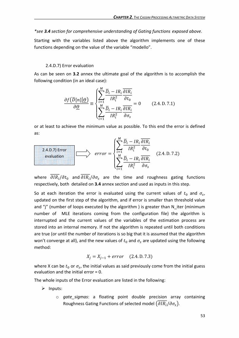
CHAPTER 2. THE CASSINI PROCESSING ALTIMETRIC DATA SYSTEM
53
*see 3.4 section for comprehensive understanding of Gating functions exposed above.
Starting with the variables listed above the algorithm implements one of these
functions depending on the value of the variable “modello”.
2.4.D.7) Error evaluation
As can be seen on 3.2 annex the ultimate goal of the algorithm is to accomplish the
following condition (in an ideal case):
M?�)9:;<���M� �12324)9� � G��G�� MG��MK�
*���)9� � G��G�� MG��M��*���
8 � 0 �2.4. D. 7.1� or at least to achieve the minimum value as possible. To this end the error is defined
as:
¦AA@A �12324)9� � G��G�� MG��MK�
*���)9� � G��G�� MG��M��*���
8 �2.4. D. 7.2� where MG��/MK� and MG��/M�� are the time and roughness gating functions
respectively, both detailed on 3.4 annex section and used as inputs in this step.
So at each iteration the error is evaluated using the current values of K� and ��,
updated on the first step of the algorithm, and if error is smaller than threshold value
and “j” (number of loops executed by the algorithm ) is greater than N_iter (minimum
number of MLE iterations coming from the configuration file) the algorithm is
interrupted and the current values of the variables of the estimation process are
stored into an internal memory. If not the algorithm is repeated until both conditions
are true (or until the number of iterations is so big that it is assumed that the algorithm
won’t converge at all), and the new values of K� and �� are updated using the following
method: �= � �=7� � ¦AA@A �2.4. D. 7.3� where X can be K� or ��, the initial values as said previously come from the initial guess
evaluation and the initial error = 0.
The whole inputs of the Error evaluation are listed in the following:
� Inputs:
o gate_sigmas: a floating point double precision array containing
Roughness Gating Functions of selected model �MG��/M���.
2.4.D.7) Error
evaluation

CHAPTER 2. THE CASSINI PROCESSING ALTIMETRIC DATA SYSTEM
54
o gate_time: a floating point double precision array containing Time
Gating Functions of selected model �MG��/MK��.
o impulse: a floating point double precision array containing the averaged
range compressed burst �):;<�.
o Variables listed in table 2.8, mainly the impulse response �G��. o tauzero_ML: already detailed
o sigma_h: already detailed
The whole outputs of the Surface Parameters Estimation tool are listed in the
following:
Variables Structure Value/Unit Reference
tauzero_ML_1step [Array] Floating point double precision [s]
error_min_tau [Array] Floating point double precision [s]
amp_ML_1step [Array] Floating point double precision
error_min_amp [Array] Floating point double precision
modello_fin_1step [Array] Floating point double precision
tauzero_ML_2step [Array] Floating point double precision [s]
amp_ML_2step [Array] Floating point double precision
error_min_amp_2step [Array] Floating point double precision
error_min_tau_2step [Array] Floating point double precision [s]
error_min_sigma_h_2step [Array] Floating point double precision [m]
modello_fin_2step [Array] Floating point double precision
sigmas_ML [Array] Floating point double precision [m]
rtt_std Floating point double precision [m]
Table 2.10 Outputs of the Surface Parameters Estimation Tool
In the following each variable will be described with more detail:
• tauzero_ML_1step: a floating point double precision array containing MLE
estimated centroid position after 1st loop.
• error_min_tau: a floating point double precision array containing MLE
convergence errors.
• amp_ML_1step: a floating point double precision array containing MLE
estimated amplitude after first loop.
• error_min_amp: a floating point double precision array containing MLE
convergence errors.
• modello_fin_1step: a floating point double precision array containing
theoretical selected model after first loop.
• tauzero_ML_2step: a floating point double precision array containing MLE
estimated centroid position after 2nd loop.
• amp_ML_2step: a floating point double precision containing MLE estimated
amplitude after 2nd loop.

CHAPTER 2. THE CASSINI PROCESSING ALTIMETRIC DATA SYSTEM
55
• error_min_amp_2step: a floating point double precision array containing MLE
convergence errors.
• error_min_tau_2step: a floating point double precision array containing MLE
convergence errors.
• error_min_sigma_h_2step: a floating point double precision array containing
MLE convergence errors.
• modello_fin_2step: a floating point double precision array containing
theoretical selected model after second loop.
• sigmas_ML: a floating point double precision array containing MLE estimated
roughness
• rtt_std: a floating point double precision array containing Estimated standard
deviation of the residual error in the range_to_target measurement. This is
required for PT ABDR production functionality
2.4.D.8) Parameters estimation: final considerations
An example of fitting of Cassini LBDR data from Ta fly-by (burst #14331) with the
Prony’s Method model described in 3.3.4 is reported in the following. The ML
estimator is initialized with the values of COG position (i.e. K̂� ¤ ?� � 500).
The analytical values used at first attempt ensure the convergence within a limited
number of steps.
The results of the iterative cycle are shown in the following figures for the first and the
last step of the process, respectively:
Figure 2.22 MLE first step (ξ=0.8908°, h =5083.2 km)

CHAPTER 2. THE CASSINI PROCESSING ALTIMETRIC DATA SYSTEM
56
An example of fitting of real data from Ta fly-by (burst #14364), after the application of
the MLE algorithm, with both nadir and off-nadir Prony’s method models is reported in
next figure, in order to evidence the differences in between:
The errors in best fitting process trend asymptotically to zero, as showed in the
following figure, in fact a typical process of convergence requires a number of
iterations not greater than 10:
Figure 2.23 MLE last step (ξ=0.8908°, h =5083.2 km)
Figure 2.24 Fitting of models with LBDR data (ξ=0.23°, h=5500km)

CHAPTER 2. THE CASSINI PROCESSING ALTIMETRIC DATA SYSTEM
57
However, sporadically the following anomalies have been identified into the Cassini
range compressed pulse:
• Echoes spreading (see figure 2.26)
• Double peaks into the 3dB pulse band (see figure 2.27)
• Secondary lobes (see figure 2.27)
Figure 2.25 MLE Best fitting process: error convergence. (It is evident that at
iteration 10th the error is practically zero)
Figure 2.26 Example of fitting impulse spreader. It is possible to note that theoretical models is not
able to fit the pulse (which is “larger” than the theoretical one)
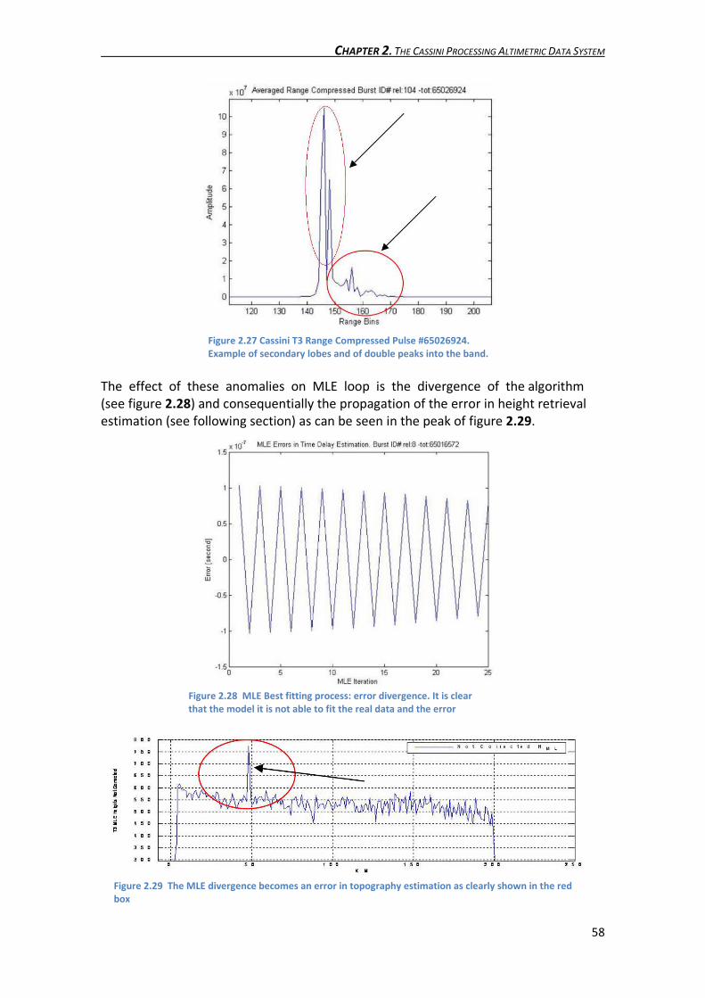
CHAPTER 2. THE CASSINI PROCESSING ALTIMETRIC DATA SYSTEM
58
The effect of these anomalies on MLE loop is the divergence of the algorithm
(see figure 2.28) and consequentially the propagation of the error in height retrieval
estimation (see following section) as can be seen in the peak of figure 2.29.
Figure 2.28 MLE Best fitting process: error divergence. It is clear
that the model it is not able to fit the real data and the error
diverges.
Figure 2.29 The MLE divergence becomes an error in topography estimation as clearly shown in the red
box
Figure 2.27 Cassini T3 Range Compressed Pulse #65026924.
Example of secondary lobes and of double peaks into the band.

CHAPTER 2. THE CASSINI PROCESSING ALTIMETRIC DATA SYSTEM
59
2.4.E) Height Retrieval
This tool provides the final values to be filled in the fields of the Science Data Segment
required for the ABDR production tool.
Starting from Time delay variables, the topographic heights are evaluated by
subtracting the range derived by taking into account the time delay pulses propagation
time-delay between transmission and reception of pulses from spacecraft altitude with
respect to the surface (i.e. orbital range-Titan mean radius) satellite orbital range to
target, to finally provide the topographic heights of Titan’s surface. The topographic
heights are the surface relative elevation respect to Titan mean equatorial radius
(R_Tit=2575 Km).
In order to synchronize the burst in terms of time delay, it is necessary to know at least
one pulse centroid position exactly, i.e. without ambiguity in term of PRIs. For
instance, the burst with the minimum number of received pulses must be process
first, thus allowing to synchronize all the other positions with respect to it. In other
words, the burst with the minimum number of received pulses is used to solve the PRI
ambiguity.
The whole inputs/outputs of this function are listed in the following:
� Inputs:
Variables Structure Value/Unit Reference
Tauzero_ML [Array] Floating point double precision [s]
H Floating point double precision. Non negative value [m]
rx_window_delay [Array] Floating point double precision [s]
Radius Short Integer. Non negative Value [m]
Range_proc [Bidimensional
Array] Floating point double precision.
Table 2.11 Input variables of Height Retrieval
� Outputs:
Variables Structure Value/Unit reference
H_ML [Array] Floating point double precision [m]
Range_2_target [Array] Floating point double precision [m]
altimeter_profile_length Short Integer
altimeter_profile_range_start Floating point double precision
altimeter_profile_range_step Floating point double precision
Table 2.12 Output variables of Height Retrieval
where:
• H_ML: is an array containig the Topographic Profile, i.e. the final altitudes,
calculated as can be seen in the following paragraphs.
• Range_2_target: this is an array containing the Range S/C to target.
• altimeter_profile_length: this is an integer containing the number of valid
entries in altimeter profile.
• altimeter_profile_range_start: a floating point double precision containing the
range of the first altimeter profile value in each pulse.

CHAPTER 2. THE CASSINI PROCESSING ALTIMETRIC DATA SYSTEM
60
• altimeter_profile_range_step: a floating point double precision containing the
difference in range between consecutive range bins in altimeter profile.
The procedure followed to obtain the topographic heights is described in the
following:
For the altimetry high resolution mode, typically:
• PRI = (1/4700 – 1/5000)s
• Pulse length = 150us
• BRI = 3333ms
• K� = rx_window_delay + t_centroid
• nº of pulses = 15
Starting with variables of table 2.11 the process starts by calculating the first range,
calculated with the burst with the minimum number of received pulses. In this way it is
possible to solve the PRI ambiguity since we are able to identify one single burst
among all the others present in the intermediate BODP file, and therefore to introduce
a time reference from which all other ranges are calculated. The procedure is as
follows:
2.4.E) Height
Retrieval
Figure 2.30 Example of burst cycle time

CHAPTER 2. THE CASSINI PROCESSING ALTIMETRIC DATA SYSTEM
61
¾� � �´_AlkgÅÆ� � �Ç)� �2 � �_�gK � �¢q>P�r�c �2
where:
• � �́�c�È� � É�Æ�_!2000_��2 � �Æ�_!2000_Ê�2 � �Æ�_!2000_Ë�2 = Satellite Radius
• �Ç) � received windows delay, see figure above
• �_�gK � Titan mean equatorial radius = 2575000f
• �¢q>P�r�c � Pulse centroid position
then for the P� averaged burst: ¾� � �´_AlkgÅÆ� � �Ç)� �2 � �_�gK � �¢q>P�r�c �2 � Æ^ Ì T Ì t�G �2
where:
• T � |¾� � ¾�| � t�G��/4� • Æ^ � Æg^;�¾� �¾�7��
Finally is possible to evaluate the Range to target by performing: �l;^¦_K@_�lA^¦K � �´_AlkgÅÆ � �_�gK � ¾�
It is worth noting that the processing takes also into account the delay due to internal
path followed by the transmitted and received signals. This time delay has been
evaluated by processing calibration data (rerouted chirp and leakage signal) and it
has been found equal to 6 µsec.
Next figure shows the topographic profiles obtained by processing of T13, T16 and T19
fly-bys, where the Titan’s height are referred to the mean planet radius:
Figure 2.31 Retrieved Titan’s surface height as a function of along track distance. The height values
are referred to Titan’s mean radius of 2575 Km (fly-bys T13, T16 and T19). The distance values are
referred to altimetric acquisition start.

CHAPTER 2. THE CASSINI PROCESSING ALTIMETRIC DATA SYSTEM
62
2.4.F) Slope Evaluation
This tool allows user to evaluate the bidirectional surface slope in the along track
direction starting from H_ML (Topographic Profile), by computing the derivative of the
estimated heights expressed in deg. The slope values have been evaluated by taking a
linear fit of the height profiles, of course considering the in-bound and out-bound part
of the trajectory separately.
The whole input/output of this function is listed in the following:
� Input: H_ML (Topographic Profile).
� Output: slope (Surface Slope [Array], Floating point double precision [m]).
2.4.G) Waveform Analysis
With this tool the user will be able to visualize the plot of the Radar Impulse Response
and the Range Compressed Data by inserting the burst ID in a dedicated edit-box. The
waveform analysis can be performed in terms of visual analysis of the shape of the
received echo waveforms for the Cassini Radar through comparison with relevant
processing parameters, on a burst basis. Thus, the SLT also allows user to plot the
following parameters:
• Pulse Repetition Interval
• Number of Transmitted/Received Pulses
• Receive Window Delay
• Time from Closest Approach
• Spacecraft Velocity in Target Body Fixed (TBF) coordinate system
• Spacecraft Range
• Off-nadir Angle
� Inputs: Range_proc and IR (Impulse Response [Array]).
The outputs of this function are on screen diagrams.
2.4.H) Performance Simulation
This tool allows user to simulate, and evaluate by means of the algorithm described in
section 2.4.D, the Cassini Radar impulse response (IR) by interactive selection of one
implemented model. The SLT allows user to select interactively the parameters to be
used for any simulation run, by choosing among:
• Spacecraft Altitude
• Off-nadir Angle
• Surface Roughness
• Surface Topography
User may execute the simulation starting from the list of the above parameters, with
current values read from PT internal files, or after setting up of new values, through
the GUI interface. This functionality allows user to visualize interactively the simulated
IR by using dedicated push-buttons in the SLT GUI interface.

CHAPTER 2. THE CASSINI PROCESSING ALTIMETRIC DATA SYSTEM
63
The whole inputs of this function are listed in the following table:
Variables Structure Value/Unit reference
t [Array] Floating Point Double Precision [s]
t0 Floating Point Double Precision [s]
gamma Floating Point Double Precision.
zita Floating Point Double Precision. Non negative value [rad]
H Floating Point Double Precision. [m]
Radius Short Integer. Non negative value [m]
sigma_c Floating Point Double Precision [s]
NN Short Integer. Min:1 Max:4
sigma_p Floating Point Double Precision. Constant Value [m]
c Floating Point Double Precision. Constant value [m]/[s]
B Floating Point Double Precision. [Hz]
Table 2.13 Inputs of Performance Simulation
The outputs of this function are on screen diagrams.
2.4.I) Results Workspace Saving
This functionality saves all the produced results in a binary format file into the local
directory. SLT Results files are automatically produced for both ALTH/AHAG operating
modes. The SLT Results file for ALTH/AHAG mode will contain the variables listed in the
following table, as noted in the introduction of the present section (2.4):
� Inputs:
Variables Structure Value/Unit reference
tauzero_ML_1step [Array] Floating Point Double precision [s]
error_min_tau [Array] Floating Point Double precision [s]
amp_ML_1step [Array] Floating Point Double precision
error_min_amp [Array] Floating Point Double precision
modello_fin_1step [Array] Floating Point Double precision
tauzero_ML_2step [Array] Floating Point Double precision
amp_ML_2step [Array] Floating Point Double precision
error_min_amp_2step [Array] Floating Point Double precision
error_min_tau_2step [Array] Floating Point Double precision [s]
error_min_sigma_h_2step [Array] Floating Point Double precision [m]
modello_fin_2step [Array] Floating Point Double precision
sigmas_ML [Array] Floating Point Double precision [m]
H_ML [Array] Floating Point Double precision [m]
slope [Array] Floating Point Double precision [deg]
Range_2_target [Array] Floating Point Double precision [m]
rtt_std Floating Point Double precision [m]
altimeter_profile_length Short Integer
altimeter_profile_range_start Floating Point Double precision
altimeter_profile_range_step Floating Point Double precision
Table 2.14 Inputs of Results Workspace Saving
The output of this function are the SLT Results files in Binary format data file.

CHAPTER 3. ANNEXES
64
3) ANNEXES
3.0) Altimetry Radar
The altimetry radar is an active sensor that operates in the microwave band. It
basically has the function to determinate its distance to the surface “illuminated” by
signals sent by the radar itself. It calculates the round trip time to the reflecting surface
since a portion of the outgoing radar signal is redirected directly back towards the
radar antenna by the target.
When a radar system transmits a pulse of energy to the ground (A), it scatters off the
ground in all directions (C). A portion of the scattered energy is directed back toward
the radar receiver (B), and this portion is referred to as "backscatter".
The accuracy, which is generally on the order of several centimeters or tens of
centimeters, depends mainly on the sharpness of the pulse, or signal bandwidth, and
the footprint of the radar beam
The backscatter is captured by the antenna, which is connected to the receiver that
detects the signal and records it to be later processed. The discrimination of the
different backscatters, received from different directions of propagation, can be
achieved with different techniques, which involve time discrimination, angular
discrimination or discrimination in terms of Doppler deviation.
The components of a radar system are:
• a pulse generator, which sends, with a certain PRF, microwave energy pulses.
• a transmitter.
• a Duplexer, which connects the antenna to the transmitter when we need to
send the pulse, and connects the antenna to the receiver when the echo must
be received.
• a directive antenna, which focuses the pulse energy into a beam.
Figure 3.1 Backscattering effect

CHAPTER 3. ANNEXES
65
• the radar echoes captured by the antenna, which are amplified and processed
appropriately.
• a data storage device, for subsequent processing (post processing).
Normally the radar transmits sinusoidal pulses of finite duration. The time between
one pulse and the following one is called repetition period � � 1/t�Í (Pulse
Repetition Frequency).
Let’s take a single sinusoidal pulse of duration j and frequency ?r, which can be
expressed as: �K� � I cos 2�?rK � j2 B K B j2 �3.0.1� It is possible to demonstrate that the bandwidth of �K� is � � 1/j. The pulse duration
is usually very short if we compare it with the repetition period, normally j*PRF=1/1000.
The time interval between the emission and the reception of the echo can be
measured with great accuracy and, therefore, if we know the propagation speed of the
electromagnetic waves in free space ( Î � � 3 Ì 10Ïm/s) we may be able to calculate
the distance R from the radar to the observed surface in the following way:
� � �ÐK2 �3.0.2� since the impulse travels a distance equal to 2R. Obviously the maximum distance that
we will be able to detect before the next pulse is transmitted by the radar will be:
�«�_ � ��2 �3.0.3� If two targets are separated by a distance ΔR, two echoes will be received by the
antenna (which has sent a single pulse), and will return to the radar with the following
temporal separation:
ÐK � 2Ð�� �3.0.4� So the pulse duration must be j � 2Ð�/� if we want to distinguish the two targets.
Thus we can define the distance resolution as the minimum distance at which two
objects can be identified as separate items: �Ñ � Ò � �j2 � �2� �3.0.5� This result shows that for good distance resolutions we should transmit pulses of very
short duration but on the other hand we also have that for great radar scopes or high
SNR’s we need long pulse durations since the energy transmitted is directly related to
this parameter. This problem will be solved with the pulse modulation technique as we
will see in the following section.
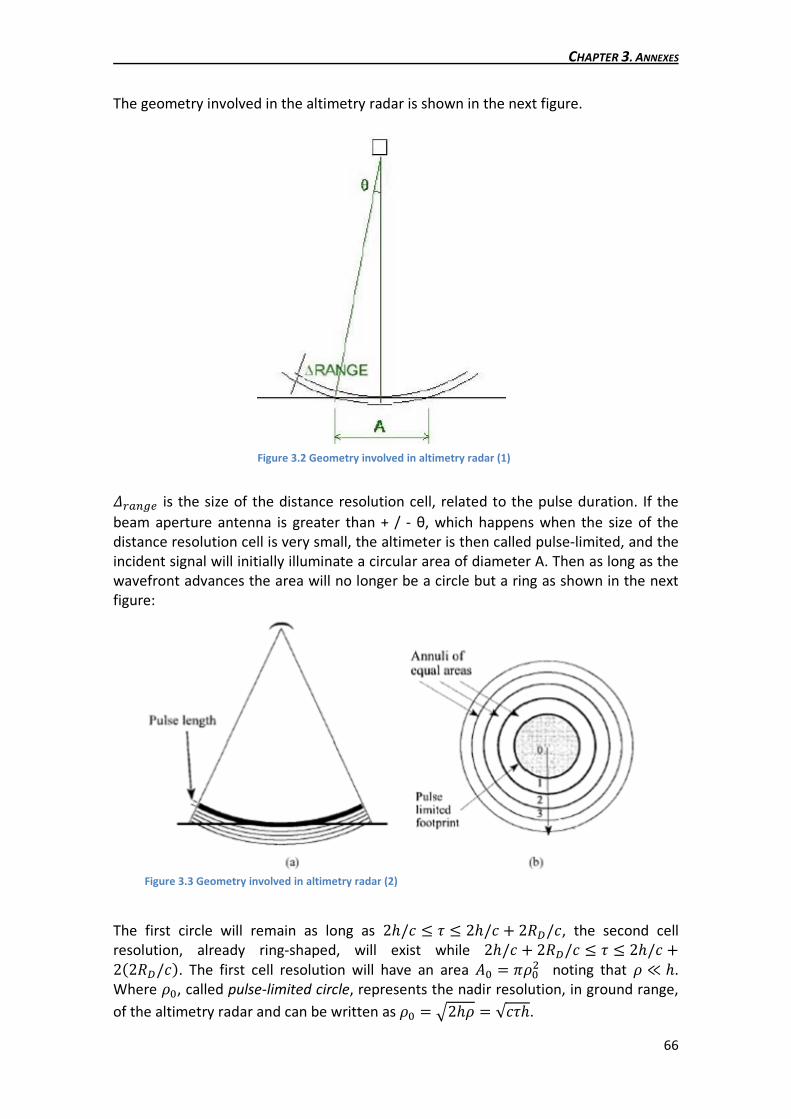
CHAPTER 3. ANNEXES
66
The geometry involved in the altimetry radar is shown in the next figure.
Ð��>Óq is the size of the distance resolution cell, related to the pulse duration. If the
beam aperture antenna is greater than + / - θ, which happens when the size of the
distance resolution cell is very small, the altimeter is then called pulse-limited, and the
incident signal will initially illuminate a circular area of diameter A. Then as long as the
wavefront advances the area will no longer be a circle but a ring as shown in the next
figure:
The first circle will remain as long as 2�/� B j B 2�/� � 2�Ñ/�, the second cell
resolution, already ring-shaped, will exist while 2�/� � 2�Ñ/� B j B 2�/� �2�2�Ñ/��. The first cell resolution will have an area I� � �Ò� noting that Ò Ô �.
Where Ò�, called pulse-limited circle, represents the nadir resolution, in ground range,
of the altimetry radar and can be written as Ò� � É2�Ò � √�j�.
Figure 3.2 Geometry involved in altimetry radar (1)
Figure 3.3 Geometry involved in altimetry radar (2)

CHAPTER 3. ANNEXES
67
As can be seen in the next figure, initially the return power increases quickly due to the
expansion of the illuminated area from a point to a circle. At that point the return
power remains constant since the area of the rings is always the same. Finally it
decreases since the ring expands up to the beam limit.
The radar echo characteristics depend mainly on the physical and geometric properties
such as shape, roughness and the dielectric constant of the observed object. In a
general way, if we consider oceanic surfaces illuminated by a pulse-limited altimetry
radar, with very small incidence angles it can be demonstrated that the return echo,
assuming a Gaussian height probability density function of the ocean, can be written as
(see Brown’s Model [8]):
t��j� Î 12324Õtptuv�0�√2��� 12 ¥1 � erf � j√2�¢ ¨ , j � 0Õtptuv�j�√2��� 12 ¥1 � erf � j√2�¢ ¨ , j d 08 �3.0.6�
where:
• Õ � �� is the compression ratio of the transmitted pulse.
• tp is the peak transmitted power.
• tuv is the average backscattered power from a mean flat surface
(illuminated by an impulse).
• ��=0.4275T and �¢ � É�� � �2��/��
In section 3.4.1 will be explained in more detail the Brown’s model and all its
assumptions and characteristics.
Brown’s Model has been widely applied to pulse-limited radar altimeters devoted to
nadir oceans observations, for Earth observation purposes, in order to map the Earth’s
geoid, to study oceanic processes, to obtain topographic details of sea surfaces. The
Figure 3.4 Brown's Model: Nadir pointed real Impulse Response of a
surface with negligible slope

CHAPTER 3. ANNEXES
68
values of the backscattering coefficient of the illuminated surface ����, the surface
roughness ���� and the time delay between surface and orbit (K�) can be obtained by
fitting the received echoes with the theoretical Brown’s Model. Once we get the value
of K� we can determine the range to the ocean and if we know the satellite’s orbit we
can obtain the average height of the observed surface by subtracting the two
distances.
In the following figures can be seen the variation of the theoretical impulse response
of Brown’s Model with respect to ��, ��, and K� respectively
3.1) Range Processing
Once we have stored the sampled echo data from the LBDR file we need to process it,
in order to be able to detect the real echoes from Titan’s surface in such a way that we
have as few as possible false detections and the distance resolution achieved is as
small as possible. In the following paragraphs will be described the physical and
mathematical concepts that lead us to choose the more appropriate filter and signal
waveform for this purpose.
The problem is then approached from two different points of view. On one hand we
are trying to find the optimal linear filter that maximizes the signal to noise ratio (SNR),
Figure 3.5 theoretical impulse response of Brown’s Model with respect to ×Ø, ×�, and Ù� respectively

CHAPTER 3. ANNEXES
69
and on the other we are trying to find the best transmitted signal waveform in order to
achieve the best distance resolution.
3.1.1) SNR Maximization
Here we would like to find the linear filter h(t) that maximizes the SNR (Matched filter).
Taking into account the following scheme:
where s(t) is the received signal and n(t) the noise of the whole system. The output
signal can be stated (considering the linearity of the system) as:
^�K� � �Æ�K� � ;�K�� ¤ ��K� � s�Æ�j� � ;�j����K � j�kj �3.1.1�y7y
when K � K� then:
^�K�� � s��j� � ;�j����K� � j�kjy7y � ^��K�� � ^>�K�� �3.1.2�
so the SNR becomes (since n(t) can be approximated by an additive white Gaussian
noise):
�� � |^��K��| DE^> �K��F � �i Æ�j���K� � j�kKy7y � Õ2i |��K� � j�| kKy7y �3.1.3� where, taking into account the Cauchy-Schwarz Inequality:
Ús ���K�� �K�kKy7y Ú B s |���K�| kKy
7y s |� �K�| y7y kK �3.1.4�
the SNR becomes
�� B i |Æ�j�| kKPQ� i |��K� � j�| PQ� kKÕ2i |��K� � j�| kKPQ� � 2Õs |Æ�j�| kK �3.1.5�PQ�
obviously the equality of the function is fulfilled when: �¤�K� � j� � Æ�j� @A ��K� � Ƥ�K� � K� �3.1.6�
g(t)
n(t)
s(t) ��K�

CHAPTER 3. ANNEXES
70
so as it can be seen the filter that maximizes the signal to noise ratio is actually the
conjugate of the signal itself inverted and shifted K� seconds.
3.1.2) Chirp Pulse Compression
If we use a sinusoidal rectangular pulse, in order to achieve a good distance resolution
we need short pulse durations, instead long pulse durations are needed if we want to
reach great radar scopes. This problem can be solved, as we will see in the following,
with the pulse compression technique.
In fact, as noted in 3.0 if we use:
Æ�K� � Û ¡K�£ cos�2�?�K� �3.1.7� where ?� is the signal frequency, we have that B = 1/T. As can be seen in 3.0.5 the
distance resolution is given by:
�Ñ � �2� � ��2
On the other hand if we consider a signal such as:
Æ�K� � IÛ ¡K�£ ¦= ÜÝQP¦=ÜÞPß �3.1.14� known as chirp pulse, where o is known as chirp rate. The phase and instantaneous
frequency of a chirp signal are given respectively by:
¿à�K� � 2�?�K � �oK ?�K� � àá2� � ?� � oK � �2 B K B �28 �3.1.15� so:
â?«�> � ?� � o �2?«�_ � ?� � o �28 �3.1.16�
and thus we have that: � � ?«�> � ?«�_ � o� �3.1.17� In this case the signal bandwidth and the pulse duration are directly proportional and
thus the distance resolution is given by:
�Ñ � �2� � �2o� �3.1.18� so in this case we can reach good distance resolutions by increasing the pulse duration,
which at the same time increases the radar scope.

CHAPTER 3. ANNEXES
71
In the following figures is presented the main structure of the chirp pulse:
?«�_
?«�>
b) Linearly frequency
modulation
Figure 3.6 Qualitative structure of a chirp signal.
K
K
K
K
c) Transmitted waveform
a)Transmitted pulse
B
Frequency
d) Received waveform
T
Amplitude
Figure 3.7 Chirp signal as a function of time

CHAPTER 3. ANNEXES
72
Let’s now make a review of the whole system. The system is, as deduced from the two
previous paragraphs, the following:
where “BB” indicates Base-Band, this is the signal after the down conversion, and:
����K� Î Û ¡K � K�� £ ¦7= ÜÝQPQ¦=ÜÞ�P7PQ�ß l;k K� � 2�� �3.1.19� it can be demonstrated that:
����?� Î Û �K[� ¦=ÜÝßÞ ågK� K[ � ?o �3.1.20� in that case, the signal output �?� will be, since in the frequency domain ¾�?� ����¤ �?�: �?� � ����?� Ì ���¤ �?� � |����?�| �3.1.21� so in the time domain, it can be showed that Ê�K� Î ��Æg;����K � K��� �3.1.22�
����K� Ê�K� ��K� � ���¤ ��K� Matched Filter:
Figure 3.8 Frequency domain chirp spectrum
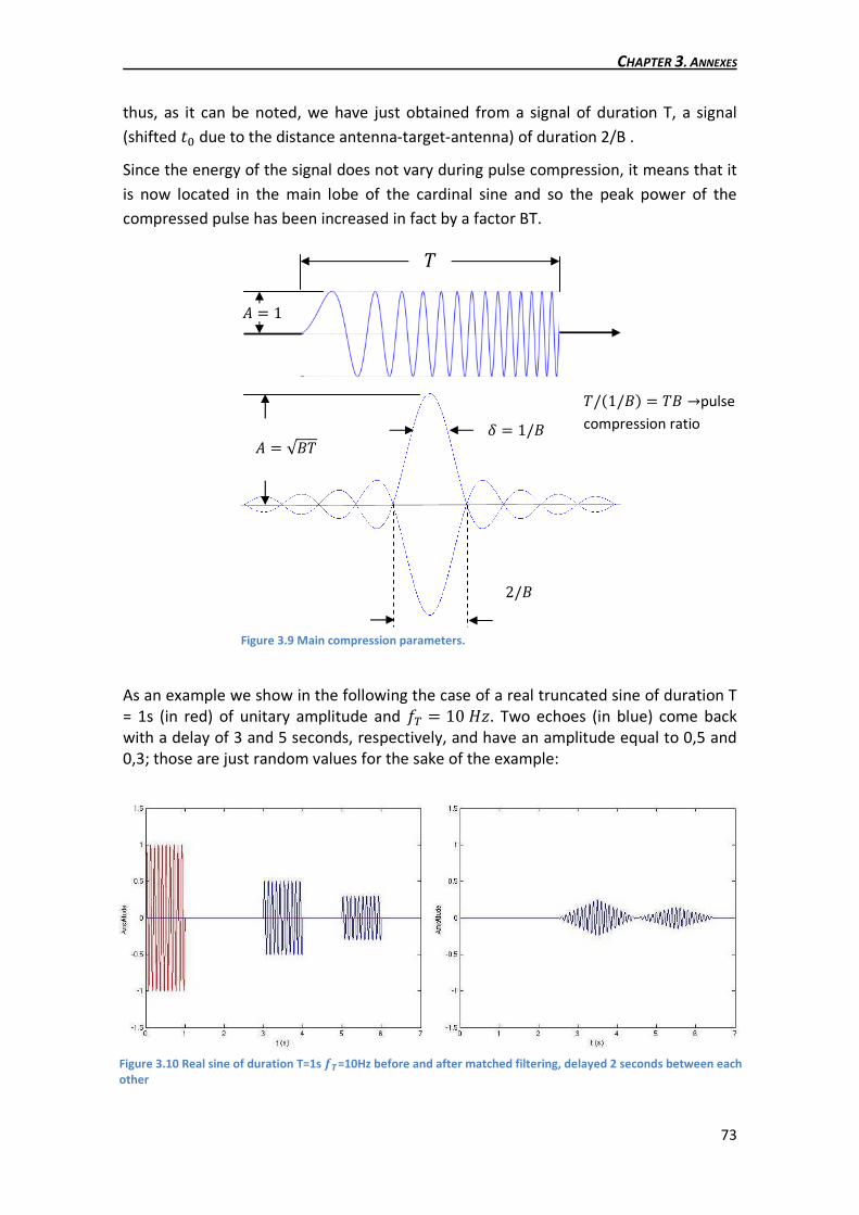
CHAPTER 3. ANNEXES
73
thus, as it can be noted, we have just obtained from a signal of duration T, a signal
(shifted K� due to the distance antenna-target-antenna) of duration 2/B .
Since the energy of the signal does not vary during pulse compression, it means that it
is now located in the main lobe of the cardinal sine and so the peak power of the
compressed pulse has been increased in fact by a factor BT.
As an example we show in the following the case of a real truncated sine of duration T
= 1s (in red) of unitary amplitude and ?p � 10 ¾Ë. Two echoes (in blue) come back
with a delay of 3 and 5 seconds, respectively, and have an amplitude equal to 0,5 and
0,3; those are just random values for the sake of the example:
�
Figure 3.9 Main compression parameters.
�/�1/�� � �� æpulse
compression ratio
I � 1
U � 1/�
2/�
I � √��
Figure 3.10 Real sine of duration T=1s ��=10Hz before and after matched filtering, delayed 2 seconds between each
other

CHAPTER 3. ANNEXES
74
If two pulses come back (nearly) at the same time, the intercorrelation is equal to the
sum of the intercorrelations of the two elementary signals. To distinguish one
"triangular" envelope from that of the other pulse, it is clearly visible that the times of
arrival of the two pulses must be separated by at least T so that the maxima of both
pulses can be separated. If this condition is false, both triangles will be mixed together
and impossible to separate:
On the other hand, if we transmit a chirped pulse (carrier 10 hertz, modulation on 16
hertz, amplitude 1, duration 1 second), we have:
3.2) MLE structure
In order to obtain the key parameters of Titan’s surface it is needed to fit the received
echoes with the theoretical models, so we are dealing now with the problem of
estimation of such parameters from real data acquired by the radar, that are affected
by thermal noise and, mainly, by speckle.
In the case of Cassini PAD system it has been chosen a Maximum Likelihood Estimation
(MLE) since this method exhibits several characteristics which can be interpreted to
Figure 3.11 Real sine of duration T=1s ��=10Hz before and after matched filtering, delayed 1 second between each
other, before and after matched filtering
Figure 3.12 Chirped pulse fo=10Hz, B=16Hz, A=1 T=1 before and after matched filtering
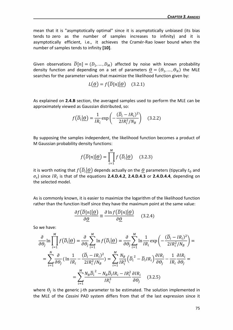
CHAPTER 3. ANNEXES
75
mean that it is "asymptotically optimal" since it is asymptotically unbiased (its bias
tends to zero as the number of samples increases to infinity) and it is
asymptotically efficient, i.e., it achieves the Cramér-Rao lower bound when the
number of samples tends to infinity [10].
Given observations )9:;< � �)�, … , )*� affected by noise with known probability
density function and depending on a set of parameters � � ���, … , ��� the MLE
searches for the parameter values that maximize the likelihood function given by: ���� � ?�)9:;<��� �3.2.1�
As explained on 2.4.B section, the averaged samples used to perform the MLE can be
approximately viewed as Gaussian distributed, so:
?�)9���� � 1G�� exp �� �)9� � G��� 2G�� /� �3.2.2�
By supposing the samples independent, the likelihood function becomes a product of
M Gaussian probability density functions:
?�)9:;<��� �ç?*��� �)9���� �3.2.3�
it is worth noting that ?�)9���� depends actually on the � parameters (tipycally K� and ��) since G�� is that of the equations 2.4.D.4.2, 2.4.D.4.3 or 2.4.D.4.4, depending on
the selected model.
As is commonly known, it is easier to maximize the logarithm of the likelihood function
rather than the function itself since they have the maximum point at the same value: M?�)9:;<���M� � M ln ?�)9:;<���M� �3.2.4� So we have: MM�= ln�)9���� � MM�=ln?�)9���� � MM�=
*���
*��� ln 1G�� exp �� �)9� � G��� 2G�� /� *
��� �
� MM�= � ln 1G�� � �)9� � G��� 2G�� /� ����� � �G��� è)9� � )9�G��é MG��M�=
*��� � 1G�� MG��M�= �
��)9� � �)9�G�� � G�� G��� MG��M�=*��� �3.2.5�
where �= is the generic j-th parameter to be estimated. The solution implemented in
the MLE of the Cassini PAD system differs from that of the last expression since it

CHAPTER 3. ANNEXES
76
would yield potential instabilities mainly caused by the presence of amplitude terms in
the derivative of the model used such as the two-way path loss ��.
To this end, the MG��/ M�= has been replaced by: MG��M�= � MG��/M�=max ¡MG��M�= £ �3.2.6� and the G�� has been neglected in the numerator of 3.2.5 since it is not multiplied by �. This sub-optimal strategy yields the actual equations of the implemented MLE:
1223224)9� � G��G�� MG��M��
*��� 6)9� � G��G�� MG��M��*���
8 �3.2.7�
It is worth noting that, as can be seen in the following section, for Cassini radar
system, the IR function mainly depends on surface backscattering, radar round-
trip time, off-nadir angle and surface height root standard deviation. This means
that MLE can allow, in principle, estimation of all these parameters and not only of the
surface height through radar round-trip time, yielding additional useful information
for characterizing the planet’s surface. This document details only the estimation of K� and ��, but the normalized backscatter cross-section �r can be also estimated with
the same procedure with the data obtained from the scatterometer measurement
So in the final step of the MLE algorithm, error is evaluated by implementing the
following system of equations with the current values of the K� and �� variables:
M?�)9:;<���M� �12324)9� � G��G�� MG��MK�
*���)9� � G��G�� MG��M��*���
8 � 0 �3.2.13�
3.3) Implemented Models
The information content held by the received echo can be extracted only by obtaining
a complete model of the altimeter’s echo waveform, since the characteristics of
the altimeter waveform are strongly related to surface characteristics (i.e.
roughness, rms slope, etc.).
In 1977, G. S. Brown proposed a theoretical model of the average impulse response of
a rough surface, the so-called Brown’s model, which has been widely applied to pulse-
limited radar altimeters devoted to nadir oceans observations but due to mission
constraints, the Cassini Radar ALT is settled to work in such a way that the pulsewidth-

CHAPTER 3. ANNEXES
77
limited and the beam-limited circles are comparable. Consequently some of the
general assumptions at the basis of the conventional models are no longer applicable.
Moreover, the geometry involved, mainly the effective attitude of the Cassini orbiter
during the hyperbolic Titan fly-bys and the not negligible off-pointing angles (which are
expected to be typically up to 0.5 degrees), will affect significantly the waveform
shape, and hence the final altimetric measurements. This implies the need for an
approximation of the surface impulse response, which incorporates all those effects
and admits a friendly closed form solution. Due to the strong dependence of the
waveform shape with the pointing angle, one model will be selected from among the
three available depending on its value.
In the following is presented a complete review of the physical concepts on which the
implemented models are based as well as a detailed review of the three models.
3.3.1) Brown’s Model
In 1967 and 1971 some authors [2] and [3], starting from the same hypotheses made
by Moore and Williams [1], demonstrated that for a rough scattering surface (a surface
appears "rough" to microwave illumination when the height variations become larger
than a fraction of the radar wavelength. The fraction is qualitative, but may be shown
to decrease with incidence angle), the average return power as a function of delay is,
when one accounts for the vertical distribution of the surface height and the radar
receiver effects, a convolution of the radar system point target response with the
average surface impulse response.
The general assumptions at the basis of the convolutional model of near normal
incidence rough surface are:
• The scattering surface may be considered to comprise a sufficiently large
number of random independent scattering elements.
• The surface height statistics are assumed to be constant over the total
area illuminated by the radar during construction of the mean return.
• The scattering is a scalar process with no polarization effects and is
frequency independent
• The variation of the scattering process with angle of incidence (relative
to the normal to the mean surface) is only dependent upon the
backscattering cross section per unit scattering area, ��, and the
antenna pattern.
• The total Doppler frequency spread �4H�/�� due to a radial velocity H�,
between the radar and any scattering element on the illuminated surface
is small relative to the frequency spread of the envelope of the
transmitted pulse (2/T, where T is the width of the transmitted pulse).
The average surface impulse response may, in turn, be represented as a convolution of
the probability density function of the height of the specular points on the surface with
the quantity defined by Moore and Williams which depends upon ��, the antenna
gain, and the range from the radar to any point on the scattering surface, referred
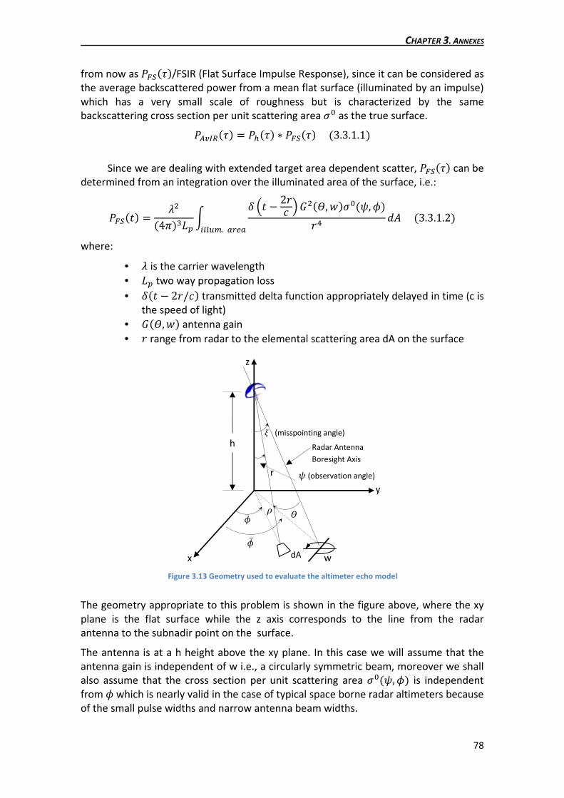
CHAPTER 3. ANNEXES
78
�
à̀
w
Ò à
z
y
x
ê (observation angle)
dA
V (misspointing angle)
r
h Radar Antenna
Boresight Axis
from now as tuv�j�/FSIR (Flat Surface Impulse Response), since it can be considered as
the average backscattered power from a mean flat surface (illuminated by an impulse)
which has a very small scale of roughness but is characterized by the same
backscattering cross section per unit scattering area �� as the true surface. t©ëxì�j� � t��j� ¤ tuv�j� �3.3.1.1�
Since we are dealing with extended target area dependent scatter, tuv�j� can be
determined from an integration over the illuminated area of the surface, i.e.:
tuv�K� � � �4�����s U èK � 2A� é � ��,å����ê, à�Aí kI �3.3.1.2��îîÈ«. ��q�
where:
• � is the carrier wavelength
• �� two way propagation loss
• U�K � 2A/�� transmitted delta function appropriately delayed in time (c is
the speed of light)
• ���,å� antenna gain
• A range from radar to the elemental scattering area dA on the surface
The geometry appropriate to this problem is shown in the figure above, where the xy
plane is the flat surface while the z axis corresponds to the line from the radar
antenna to the subnadir point on the surface.
The antenna is at a h height above the xy plane. In this case we will assume that the
antenna gain is independent of w i.e., a circularly symmetric beam, moreover we shall
also assume that the cross section per unit scattering area ���ê, à� is independent
from à which is nearly valid in the case of typical space borne radar altimeters because
of the small pulse widths and narrow antenna beam widths.
Figure 3.13 Geometry used to evaluate the altimeter echo model

CHAPTER 3. ANNEXES
79
Now if we consider that kI � Ò kÒkà, we just need to determine the � angle as a
function of Ò and à to complete the à-integration in 3.3.1.2. Using the law of cosines
and some trigonometrical identities we find:
�@Æ� � cos V � O sin V cos�à̀ � à�√1 � O �3.3.1.3� where O � Ò/�.
Using a Gaussian approximation to the antenna gain (generally valid out to the point
on the antenna pattern for which there is no appreciable contribution to the
backscattered power):
���� Î �� exp ¡�2¬ sin �£ �3.3.1.4� where ¬ � �2èsin èïðñ, é / ln 0.5é and with A � É� � Ò , 3.3.1.2 can be written as:
tuv�K� � �� � �4�����s s U èK � 2�� √1 � O é�1 � O � ���ê� Ü�
y� ¤
¤ exp L�4¬ �1 � cos V1 � O � ² � l cos�à̀ � à� � ² sin �à̀ � à�N kàÒkÒ �3.3.1.5� where:
• l � �4O/¬��sin 2V /�1 � O ��
• ² � �4O /¬��sin V /�1 � O ��
Because of the 2� range of the integration and the form of the integrand, the à̀ angle
can be ignored, thus substituting:
exp��² sin �à�� � ��1�>²> sin òà;!y>�� �3.3.1.6�
the equation 3.3.1.5 becomes
tuv�K� � 2√��� � ���ê���4������í ��1�>ô�; � 1/2�ô�; � 1�y>�� ¤
¤ s ¡2²l £> G>�l� exp ¥�4¬ �1 � cos ξ�1 � O � � ²¨y�
U èK � 2�� √1 � O é�1 � O � ÒkÒ �3.3.1.7�
since:
s exp�l cos à � ² sin à�kà � 2√� Ü� ��1�>ô�; � 1/2�ô�; � 1� ¡2²l £> G>�l� �3.3.1.8�y
>��

CHAPTER 3. ANNEXES
80
where G>�Ì� are the modified Bessel function of order n, and ô�Ì� are gamma
functions.
Then under a suitable change of variables 3.3.1.7 can be evaluated, and taking into
account that for space borne altimetry �j/� Ô 1, we obtain, in term of the two-way
incremental ranging time i.e., j � K � K� � K � 2�/� (do not confound this j with that
of the 3.0 section):
tuv�j� � �� � ����ê��4�4�� ���� exp ö� 4¬ sin V � 4�¬� j cos 2V÷ ¤
¤ L��1�>ô�; � 1/2�ô�; � 1� ¥$�j� tan V¨> G> �4¬ $�j� sin 2V N �3.3.1.9�y>��
for j d 0 and tuv�j� � 0 for j d 0.
Now if we rewrite:
EÌF � G�� � ù1 ����1�>ô�; � 1/2�ô�; � 1� G>� �G�� � ö ¬ 8 cos V÷> y>�� ú �3.3.1.10�y
>��
where:
� 4¬$�j� sin 2V �3.3.1.11� we can easily see that for �¬ �/�8 cos V� Ô 1 the series becomes highly convergent
due to rapidly decreasing (with n) of :�¬ �/�8 cos V�<>, so for:
$�j� tan V Ô 1 �3.3.1.12� the infinite series in 3.4.1.9 may be truncated at n=0 with no effective loss in accuracy,
thus finally:
¿tuv�j� � �� � ����ê��4�4�� ���� exp ¡�4¬ sin ξ � 4�j¬� �@Æ 2V£ Gr �4¬ Æg; 2V $�j� j d 0tuv�j� � 0 j � 0 �3.3.1.13� 8 where tanê� Î É�j/�. It is interesting to note that this condition under which
3.3.1.13 is valid, depends on the altitude and the pointing angle but not on the
antenna pattern.
As pointed before, in order to obtain the average return power the FSIR must be
convoluted with the probability density function of the height of the specular points on
the surface and with the radar system point target response: G��j� � tuv�j� ¤ t��j� ¤ t��j� �3.3.1.14�
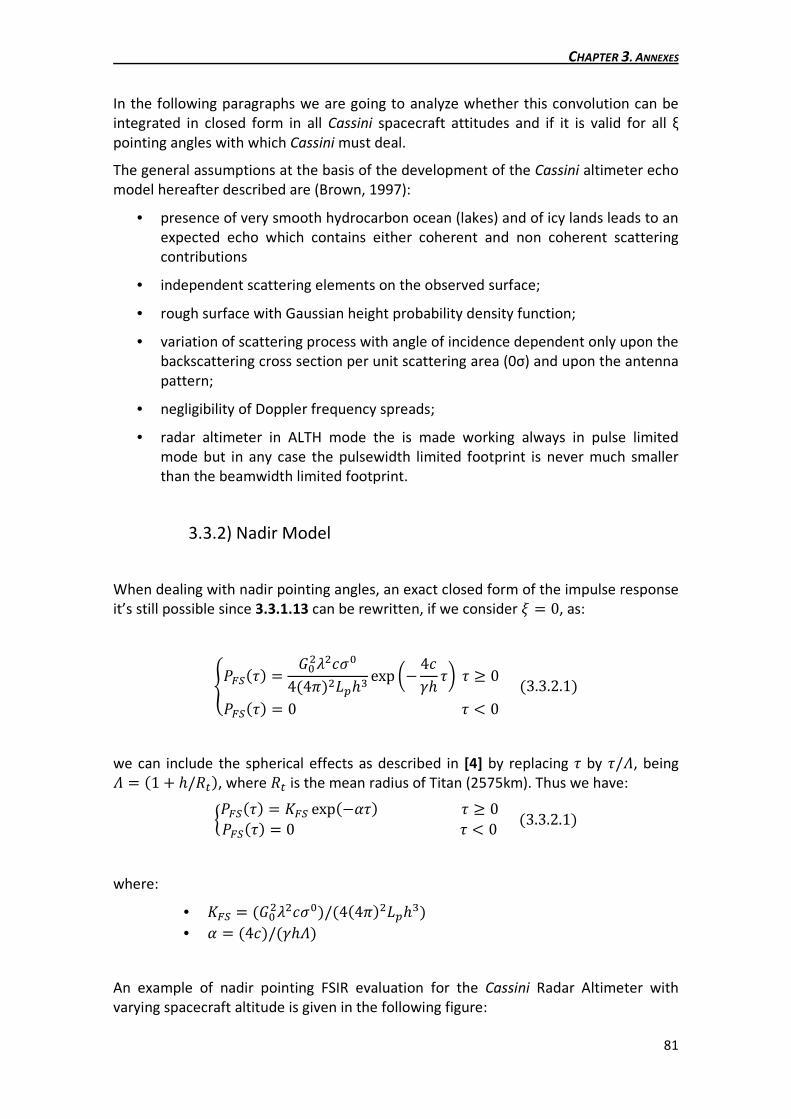
CHAPTER 3. ANNEXES
81
In the following paragraphs we are going to analyze whether this convolution can be
integrated in closed form in all Cassini spacecraft attitudes and if it is valid for all ξ
pointing angles with which Cassini must deal.
The general assumptions at the basis of the development of the Cassini altimeter echo
model hereafter described are (Brown, 1997):
• presence of very smooth hydrocarbon ocean (lakes) and of icy lands leads to an
expected echo which contains either coherent and non coherent scattering
contributions
• independent scattering elements on the observed surface;
• rough surface with Gaussian height probability density function;
• variation of scattering process with angle of incidence dependent only upon the
backscattering cross section per unit scattering area (0σ) and upon the antenna
pattern;
• negligibility of Doppler frequency spreads;
• radar altimeter in ALTH mode the is made working always in pulse limited
mode but in any case the pulsewidth limited footprint is never much smaller
than the beamwidth limited footprint.
3.3.2) Nadir Model
When dealing with nadir pointing angles, an exact closed form of the impulse response
it’s still possible since 3.3.1.13 can be rewritten, if we consider V � 0, as:
¿tuv�j� � �� � ���4�4�� ���� exp ¡� 4�¬� j£ j d 0tuv�j� � 0 j � 08 �3.3.2.1�
we can include the spherical effects as described in [4] by replacing j by j/û, being û � �1 � �/�P�, where �P is the mean radius of Titan (2575km). Thus we have:
Wtuv�j� � Tuv exp��oj� j d 0tuv�j� � 0 j � 0 8 �3.3.2.1�
where:
• Tuv � ��� � ����/�4�4�� ����� • o � �4��/�¬�û�
An example of nadir pointing FSIR evaluation for the Cassini Radar Altimeter with
varying spacecraft altitude is given in the following figure:

CHAPTER 3. ANNEXES
82
The width of each waveform sampling gate is 30m, corresponding to the vertical
resolution of the Hi-Res Altimeter (ALT) of the Cassini Radar, which is given by �/�2?¢� Î 30m, where ?¢ is the sampling frequency. In the following K� is the
reference time, i.e. the instant at which the first echo from the surface within the
radar footprint is expected to arrive. Therefore, all the functions will be centered
around this value, which at first attempt is settled to be 500 if expressed in range bins
(K� ¤ ?¢), as results from LBDR echo data.
The height probability density function and the system point target response, both
supposed to be Gaussian, are given by the following expressions:
t��j� � 1√2��� �2 exp�� j 2�� � 4 �3.3.2.2� t��j� � tp�√2��� exp �� j 2�� �3.3.2.3�
where �� is the rms height of the specular points relative to the mean surface level, tp is the peak transmitted power, and �� is related to the 37,84 dB width of the
transmitted pulse by the following relation: �� � �/√8 ln 2.
The convolution between 3.3.2.2 and 3.3.2.3 can be written as: twx�j� � Twx exp��lj � �3.3.2.4�
Figure 3.14 Nadir pointing FSIR with varying spacecraft altitude

CHAPTER 3. ANNEXES
83
where:
• Twx � tp��√2����/�¢�, • l � 1/�2�¢ � • �¢ � �� � �� • �� � ¢ ��
The total average impulse response is then given by: twx�j� ¤ tuv�j� � TuvTwx exp��oj� ¤ exp��lj � �
� TuvTwx exp��lj �s exp��2²K� exp��lK � kK �3.3.2.5�y�
where 2² � o � 2lj.
Since, as can be seen in [5]:
s exp��2²K� exp��lK �kK � 12$�l exp �² l y� ¦A?� ¡ ²√l£ �3.3.2.6�
the total average impulse response can be written as: 8G��j�|��c�� � twx�j� ¤ tuv�j� �
� T�� 12 exp �U 2 exp ¡� U�¢ j£ ¥1 � ¦A? � j√2�¢ � U√2 ¨ �3.3.2.7�
where
• U � o�¢
• T � ü�� � �/�2�4�� �����ýtp�����
This equation is not dependent of any condition about the altimeter’s operative mode,
e.g. pulse-limited or not, and it can be considered as a generalization of the Brown’s
model.
It is worth noting that if the altimeter operating conditions vary towards a typical
pulse-limited mode, then the equation 3.3.2.7 gives back the classical Brown echo,
whose validity conditions are met when the parameter δ is small (e.g. δ<<1). In that
case we have: U 2 Ô U�¢ l;k U√2 Ô j√2�¢
and so equation 3.3.2.7 becomes exactly that of the section 3.0.
For the Cassini Radar Altimeter, δ varies between 0.5 and 1.1, as shown in the
following figure:

CHAPTER 3. ANNEXES
84
Since U � o�¢, in general, the condition δ<<1 can be met if:
• o � ?�¬7��7�� is small, i.e. the spacecraft altitude h increases, given the
beamwidth and the pulse duration, and/or the antenna parameter ¬ �?���c�� increases.
• �¢ is small, i.e. the parameter �� decreases due to a greater bandwidth B.
Some case studies of echo waveforms with varying δ are shown in the following figure,
in order to perform a comparison between the IR model 3.3.2.7 and the Brown’s
model in case of nadir incidence. For the Skylab S-193 radar altimeter the following
parameters have been considered, according to Brown’s model: h=435.5km, ��c�=1.78°, ��=29.3ns:
Figure 3.15 Parameter δ versus spacecraft altitude for the Cassini Radar Altimeter
Figure 3.16 Comparison between IR models
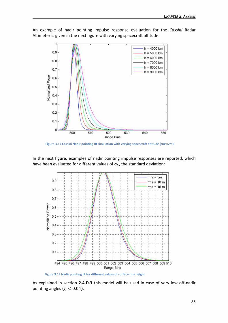
CHAPTER 3. ANNEXES
85
An example of nadir pointing impulse response evaluation for the Cassini Radar
Altimeter is given in the next figure with varying spacecraft altitude:
In the next figure, examples of nadir pointing impulse responses are reported, which
have been evaluated for different values of ��, the standard deviation:
As explained in section 2.4.D.3 this model will be used in case of very low off-nadir
pointing angles �V � 0.04�.
Figure 3.17 Cassini Nadir pointing IR simulation with varying spacecraft altitude (rms=2m)
Figure 3.18 Nadir pointing IR for different values of surface rms height

CHAPTER 3. ANNEXES
86
3.3.3) Asymptotic Brown Model
When dealing with far ξ off-nadir angles the approximation made in 3.3.1.12 is no
longer possible since the argument of the Bessel functions in 3.3.1.9 becomes very
large even for relatively small delay times (j). This large argument requires an
alternate expression for the FSIR based on asymptotic methods suggested by Brown in
1989 [7].
If we come back to equation 3.3.1.8, we see that we can also write:
s exp�l cosà � ² sin à�kà � Esin à � 1 � cos àF � Ü�
� exp��²�s exp�l cos à � ² cos à�kà �3.3.3.1�Ü7Ü
now in the right side of 3.3.3.1 it is clear that the maximum is at à � 0 so for either l
or ² or both sufficiently large, 3.3.3.1 can be asymptotically evaluated by Laplace’s
method [6] to finally give:
exp��²�s exp�l cos à � ² cos à�kà Î exp�l�� 2�l è1 � 2²l é �3.3.3.2�Ü7Ü
It is worth noting that in this last result the validity or computability of 3.3.3.2 does not
depend on which factor l or ² is larger, in contrast to what is taking place with the
series in 3.3.1.8 where is easy to compute when l þ ² but difficult when l and ² are
comparable.
At this point we can substitute 3.3.3.2 back into 3.3.1.5 and complete the Ò-
integration to yield:
tuv©�ª«��j� � �r � ���2�4������� ��O� � I����O� �3.3.3.3� where:
��O� � exp ¡� 4¬�1 � O � �sin V � O cos V� £� 2�l � 2² �3.3.3.4� in this case the parameter O has been approximated by O � É�j/�û.
As can be seen in [7] a criterion is provided which, if met, ensures that the error in
using the above approximation will be less than 2% of the true value. This criterion can
be expressed in the following form:
j«�> d �� �0.849¬ �1 � tan V�tan V

CHAPTER 3. ANNEXES
87
which shows how for a given pointing angle V, antenna beamwidth (embedded in ¬),
and radar height h, there is a minimum ranging time j«�> for which 3.3.3.3 is accurate
to less than 2% error, as indicated in the following figure:
However as noted in 2.4.D.3 section the Cassini PAD System has developed its own
method to establish the range of off-nadir angles where the asymptotic Brown Model
can be used.
For the Cassini Radar Altimeter, the value of j«�> (in range bins) with varying
spacecraft altitude and off-nadir angle is given in the following figure. As clearly
shown, the error is bounded within the first few pixels:
Figure 3.19 Error in using equation 3.3.3.3 (ξ=0.23°, h =4000 km)
Figure 3.19 Variation of ���� (in range bins) with spacecraft altitude for various off-nadir angles
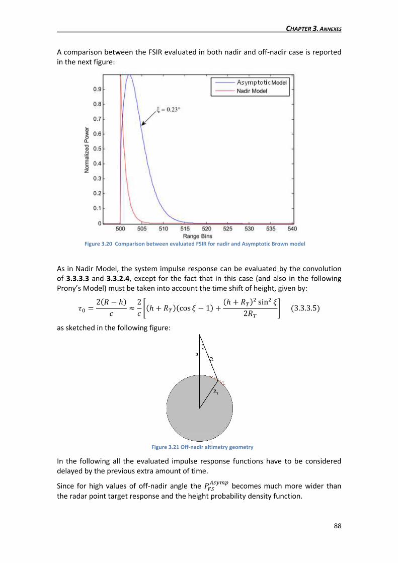
CHAPTER 3. ANNEXES
88
A comparison between the FSIR evaluated in both nadir and off-nadir case is reported
in the next figure:
As in Nadir Model, the system impulse response can be evaluated by the convolution
of 3.3.3.3 and 3.3.2.4, except for the fact that in this case (and also in the following
Prony’s Model) must be taken into account the time shift of height, given by:
j� � 2�� � ��� Î 2� ¥�� � �p��cos V � 1� � �� � �p� sin V2�p ¨ �3.3.3.5� as sketched in the following figure:
In the following all the evaluated impulse response functions have to be considered
delayed by the previous extra amount of time.
Since for high values of off-nadir angle the tuv©�ª«� becomes much more wider than
the radar point target response and the height probability density function.
Figure 3.20 Comparison between evaluated FSIR for nadir and Asymptotic Brown model
Figure 3.21 Off-nadir altimetry geometry

CHAPTER 3. ANNEXES
89
Thus the total impulse response can be simply written as the product of the following
terms: 8G��j�|©�ª«� � tuv©�ª«��j��� �1 � ¦A? è �√ R�é� �
� I����O��� ¥1 � ¦A? � j√2�¢ ¨ �3.3.3.6� This model is reported in the two following figures, for all likely scenarios in terms of
spacecraft altitude and off-pointing angle:
Figure 3.22 Asymptotic model with varying spacecraft altitude (ξ=0.23°)
Figure 3.23 Asymptotic model with varying off-nadir angle (h =4000 km)

Due to reasons mentioned above, this model will be chosen when dealing with far off
nadir values.
3.3.4) Prony’s Method Model
When dealing with small mispointing angles, we must work in such a way that the
approximation made in the previous section is no longer valid since it will produce too
big errors to deal with (see
since in this case .
In 1977 Brown made some approximations (see
exact closed form of the equation
the pulse-width limited circle is muc
unfortunately, due to mission constraints, the
such a way that the pulsewidth
so an alternative method was need
nadir angles.
The figure above shows that when operating in high resolution altimetry mode the
radar operates in the PL region but BL circle and the PL are always comparable. (where
, the pulsewidth limited circle and
limited circle)
The method, suggested by Brown in
G. Picardi and R. Seu in [9]
in 3.3.1.13 by a series of exponentials using Prony’s Method see
This method allows closing
series and yields a simple function of exponentials.
The starting point is the FSIR expression of
adimensional parameter :
Figure 3.24 Pulsewidth limited to beamwidth limited circle ratio for the
high resolution Cassini
C
Due to reasons mentioned above, this model will be chosen when dealing with far off
Prony’s Method Model
When dealing with small mispointing angles, we must work in such a way that the
approximation made in the previous section is no longer valid since it will produce too
big errors to deal with (see 2.4.D.3 section). Obviously the equation 3.3.2.1
In 1977 Brown made some approximations (see [8]) that yielded, at the end, with an
exact closed form of the equation 3.3.1.14, this approximations were possible when
width limited circle is much smaller than the beam-width limited circle. But
unfortunately, due to mission constraints, the Cassini Radar ALT is settled to work in
such a way that the pulsewidth-limited and the beam-limited circles are comparable,
so an alternative method was needed in order to manage when dealing with small off
The figure above shows that when operating in high resolution altimetry mode the
radar operates in the PL region but BL circle and the PL are always comparable. (where
ulsewidth limited circle and , the beamwidth
The method, suggested by Brown in [8] and developed by E. Montefredini, F. Morelli,
consists in approximating the Bessel function (
by a series of exponentials using Prony’s Method see [6]
closing the convolution integral for each exponential term in the
series and yields a simple function of exponentials.
point is the FSIR expression of 3.3.1.13 rewritten as a function of the
:
Pulsewidth limited to beamwidth limited circle ratio for the case of the
CHAPTER 3. ANNEXES
90
Due to reasons mentioned above, this model will be chosen when dealing with far off-
When dealing with small mispointing angles, we must work in such a way that the
approximation made in the previous section is no longer valid since it will produce too
3.3.2.1 is not valid
) that yielded, at the end, with an
, this approximations were possible when
width limited circle. But
Radar ALT is settled to work in
limited circles are comparable,
ed in order to manage when dealing with small off-
The figure above shows that when operating in high resolution altimetry mode the
radar operates in the PL region but BL circle and the PL are always comparable. (where
, the beamwidth
and developed by E. Montefredini, F. Morelli,
consists in approximating the Bessel function ( ) of the FSIR
[6] and section 3.5.
the convolution integral for each exponential term in the
rewritten as a function of the
the

CHAPTER 3. ANNEXES
91
tuv�O� � Tuv exp ¡�4¬ O cos 2V£ G� ¡4¬ O sin 2V£ �3.3.4.1�
After some trade-off (see [11]), it has been found that the most convenient way of
approximating the Bessel function is the following:
G� ¡4¬ O sin 2V£ �́ exp�l��� �3.3.4.2�����
where the constants �́ and l� are evaluated with Prony’s method of order N and � � sin�2V�O /¬ so the tuv�O� can be rewritten as:
tuv�j� � Tuv exp��T�j� �́ exp�T�j����� �3.3.4.3�
where:
134T� � 4¬ cos 2V ��û T� � 4¬ sin 2V ��û l�
8 �3.3.4.4�
The final impulse response, using Prony’s method can be written as:
8G��j�|³�r>ª � tuv�j� ¤ twx�j� �G���j� �3.3.4.5�����
where : G���j� � TuvTwx �́ exp��T�j� exp�T�j� ¤ exp��lj � � � EU� � �T� � T���¢F � TuvTwx �́ exp�U�j� ¤ exp��lj � �3.3.4.6� which is exactly like the 3.3.2.5 except for the �́ term, so we can proceed in an
analogous way and finally we have:
G���j� � �́T�� 12 exp ¡�4¬ sin V£ exp �U� 2 � U��¢ j ¤ ¤ ¥1 � ¦A? � j√2�¢ � U�√2 ¨ �3.3.4.5�
so the total impulse response for small mispointing angles calculated with Prony’s
Method can be stated as:
8G�|³�r>ª�j� � T�� 12 exp ¡�4¬ sin V£ �́exp �U� 2 � U��¢ j ¤ ����
¤ ¥1 � ¦A? � j√2�¢ � U�√2 ¨ �3.3.4.6�

CHAPTER 3. ANNEXES
92
The values of constants �́ and l�, calculated with the Prony’s method are showed in
the following table:
N=2 N=3 N=4 N=5
� 0.4931-3.0089j
0.4931+3.0089j
8.1825-0.0000j
-3.5914-0.8860j
-3.5914+0.8860j
1.6103-27.0408j
1.6103+27.0408j
-1.1103+6.7271j
-1.1103-6.7271j
1.3582-17.5134j
1.3582+17.5134j
-0.8581+4.2427j
-0.8581-4.2427j
-2.3922e-5+3.3479e-12j
�� 52.5318+25.1672j
52.5318-25.1672j
45.3668
31.7576+29.0453j
31.7576-29.0453j
31.5091+8.3585j
31.5091-8.3585j
20.4373+23.3103j
20.4373-23.3103j
34.1407+10.1205j
34.1407-10.1205j
19.7521+25.7877j
19.7521-25.7877j
-4.3681e4+9.9049e4j
Table 3.1 Exponential and amplitude factors for Prony’s approximation
3.4) Gating Functions
In the following paragraphs will be described the mathematical concepts followed to
evaluate the gating functions:
3.4.1) Nadir Model time gating function
The starting point is 3.3.2.7 equation: 8G��j�|��c�� � T�� 12 exp�U 2 exp ¡� U�¢ j£ ¥1 � ¦A? � j√2�¢ � U√2 ¨ �3.4.1.1� where j � K � 2�/� � K � K�. If we take:
� � T�� 12 exp�U 2 exp ¡� U�¢ K£ �3.4.1.2� we can rewrite 3.3.2.7 as: 8G��K��|��c�� � � exp ¡ U�¢ K�£ ¥1 � ¦A? �K � K�√2�¢ � U√2 ¨ �3.4.1.3�
By taking the derivative with respect to K� and noting that: Merf �Ë�MË � 2√� exp��Ë � �3.4.1.4� we have: M8G��K��|��c��MK� � � U�¢ exp ¡ U�¢ K�£ ¥1 � ¦A? �K � K�√2�¢ � U√2 ¨ �
�� exp ¡ U�¢ K�£ 2√� exp �� �K � K�� 2�¢ � U 2 � �K � K���¢ U �� 1√2�¢ �
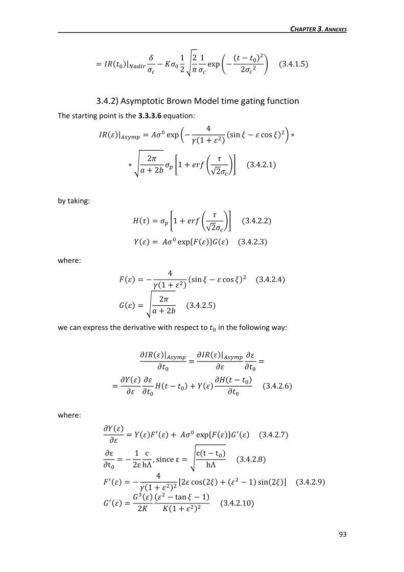
CHAPTER 3. ANNEXES
93
� 8G��K��|��c�� U�¢ � T�� 12�2� 1�¢ exp �� �K � K�� 2�¢ �3.4.1.5�
3.4.2) Asymptotic Brown Model time gating function
The starting point is the 3.3.3.6 equation: 8G��O�|©�ª«� � I�� exp ¡� 4¬�1 � O � �sin V � O cos V� £ ¤ ¤ � 2�l � 2² �� ¥1 � ¦A? � j√2�¢ ¨ �3.4.2.1�
by taking:
¾�j� � �� ¥1 � ¦A? � j√2�¢ ¨ �3.4.2.2� �O� � I�� expEÍ�O�F��O� �3.4.2.3� where:
Í�O� � � 4¬�1 � O � �sin V � O cos V� �3.4.2.4� ��O� � � 2�l � 2² �3.4.2.5�
we can express the derivative with respect to K� in the following way:
M8G��O�|©�ª«�MK� � M8G��O�|©�ª«�MO MOMK� �
� M �O�MO MOMK�¾�K � K�� � �O� M¾�K � K��MK� �3.4.2.6�
where: M �O�MO � �O�Í��O� � I�� expEÍ�O�F���O� �3.4.2.7� ∂ε∂t� � � 12ε
chΛ , since ε � �c�t � t��
hΛ �3.4.2.8� Í��O� � � 4¬�1 � O � :2O cos�2V� � �O � 1� sin�2V�< �3.4.2.9� ���O� � ���O�2T �O � tan V � 1�T�1 � O � �3.4.2.10�
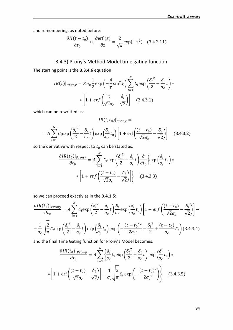
CHAPTER 3. ANNEXES
94
and remembering, as noted before: M¾�K � K��MK� � Merf �Ë�MË � 2√� exp��Ë � �3.4.2.11�
3.4.3) Prony’s Method Model time gating function
The starting point is the 3.3.4.6 equation:
8G��j�|³�r>ª � T�� 12 exp ¡�4¬ sin V£ �́exp �U� 2 � U��¢ j ¤����
¤ ¥1 � ¦A? � j√2�¢ � U�√2 ¨ �3.4.3.1� which can be rewritted as: 8G��K, K��|³�r>ª �
� A �́exp �U� 2 � U��¢ K exp ¡U��¢ K�£ ¥1 � erf ��K � K��√2�¢ � U�√2 ¨���� �3.4.3.2�
so the derivative with respect to K� can be stated as: M8G��K��|³�r>ªMK� � I �́exp �U� 2 � U��¢ K ∂∂t� Wexp ¡U��¢ K�£8
���� ¤
8¤ ¥1 � ¦A? ��K � K��√2�¢ � U�√2 ¨N �3.4.3.3�
so we can proceed exactly as in the 3.4.1.5: M8G��K��|³�r>ªMK� � I �́exp �U� 2 � U��¢ K U��¢ exp ¡U��¢ K�£ ¥1 � ¦A? ��K � K��√2�¢ � U�√2 ¨ �����
� 1�¢�2� �́exp �U� 2 � U��¢ K exp ¡U��¢ K�£ exp�� �K � K�� 2�¢ � U� 2 � �K � K���¢ U� �3.4.3.4� and the final Time Gating function for Prony’s Model becomes: M8G��K��|³�r>ªMK� � ILU��¢ �́exp �U� 2 � U��¢ K exp ¡U��¢ K�£8
���� ¤
8¤ ¥1 � erf ��K � K��√2�¢ � U�√2 ¨ � 1�¢�2� �́ exp �� �K � K�� 2�¢ ½ �3.4.3.5�

CHAPTER 3. ANNEXES
95
3.4.4) Nadir Model roughness gating function
The starting point is 3.3.2.7 equation: 8G��j�|��c�� � T�� 12 exp�U 2 exp ¡� U�¢ j£ ¥1 � ¦A? � j√2�¢ � U√2 ¨ �3.4.4.1� noting that U � o�¢ we can rewrite: 8G���¢�|��c�� � T�� 12 exp�o �¢ 2 exp��oj� ¥1 � ¦A? � j√2�¢ � o�¢√2 ¨ �
� ´ exp�o �¢ 2 ¥1 � ¦A? � j√2�¢ � o�¢√2 ¨ �3.4.4.2�
so de derivative with respect to �¢ can be written as: M8G���¢�|��c��M�¢ � ´o �¢ exp �o �¢ 2 ¥1 � ¦A? � j√2�¢ � o�¢√2 ¨ �
��2� ¡ j�¢ � o£´ exp �o �¢ 2 exp�� j 2�¢ � o �¢ 2 � oj �
� o �¢ 8G���¢�|��c�� � T�� 12�2� ¡ j�¢ � o£ exp�� j 2�¢ �3.4.4.3� finally the Roughness gating function of the Nadir Model can be written as: M8G�����|��c��M�� � M8G���¢�|��c��M�¢ M�¢M�� �3.4.4.4� where M�¢/M�� � ��/�¢ since �¢ � É�� � ��
3.4.5) Asymptotic Brown Model roughness gating function
The starting point is the 3.3.3.6 equation: 8G���¢�|©�ª«� � I�� exp ¡� 4¬�1 � O � �sin V � O cos V� £ ¤ ¤ � 2�l � 2² �� ¥1 � ¦A? � j√2�¢ ¨ �3.4.5.1�
so de derivative with respect to �¢ can be stated as: M8G���¢�|©�ª«�M�¢ � I�� exp ¡� 4¬�1 � O � �sin V � O cos V� £ ¤
¤ � 2�l � 2² �� 2√� �� j√2�¢ exp �� j 2�¢ �3.4.5.2�

CHAPTER 3. ANNEXES
96
and finally the roughness gating function of the Asymptotic Brown Model can be
expressed as: M8G�����|©�ª«�M�� � M8G���¢�|©�ª«�M�¢ M�¢M�� �3.4.5.3� where M�¢/M�� � ��/�¢.
3.4.6) Prony’s Method Model roughness gating function
The starting point is the 3.3.4.6 equation:
8G��j�|³�r>ª � T�� 12 exp ¡�4¬ sin V£ �́exp �U� 2 � U��¢ j ���� ¤
¤ ¥1 � ¦A? � j√2�¢ � U�√2 ¨ �3.4.6.1� since U� � �T� � T���¢ we can express the equation as a function of �¢:
8G���¢�|³�r>ª � I �́ exp ���T� � T��j� exp ��T� � T�� �¢ 2 ���� ¤
¤ ¥1 � erf � j√2�¢ � �T� � T���¢√2 ¨ �3.4.6.2� the derivative with respect to �¢ results to be M8G���¢�|³�r>ªM�¢ � T�� 12 exp ¡�4¬ sin V£ �́ exp ���T� � T��j��T� � T�� �¢�
��� ¤
¤ exp ��T� � T�� �¢ 2 ¥1 � erf � j√2�¢ � �T� � T���¢√2 ¨ �
��2� �́ À j�¢ � �T� � T��Á exp�� j 2 �3.4.6.3� and finally the roughness gating function of the Prony’s Model, as in the other cases,
can be expressed as: M8G�����|³�r>ªM�� � M8G���¢�|³�r>ªM�¢ M�¢M�� �3.4.6.4� where M�¢/M�� � ��/�¢.
3.5) Prony’s Method
Prony analysis is a method of fitting a linear combination of exponential terms to a
signal as shown in 3.5.1. Each term in 3.5.1 has four elements: the magnitude I>, the
damping factor �>, the frequency ?>, and the phase angle �>. Each exponential

CHAPTER 3. ANNEXES
97
component with a different frequency is viewed as a unique mode of the original
signal �K�. The four elements of each mode can be identified from the state space
representation of an equally sampled data record. The time interval between each
sample is T:
Ê�K� � I>¦R�P cos�2�?>K � �>�, ; � 1,2,3, … , �3.5.1��>��
Using Euler’s theorem and letting t=MT, the samples of Ê�K� are rewritten as:
Ê* � �>�>* �3.5.2��>��
where:
�> � I>2 ¦=ï� l;k �> � exp:��> � !2�?>��< �3.5.3� Prony analysis consists of three steps. In the first step, the coefficients of a linear
predication model are calculated. The linear predication model (LPM) of order N,
shown in 3.5.4, is built to fit the equally sampled data record �K� with length M.
Normally, the length M should be at least three tines larger than the order N: Ê* � l�Ê*7� � l Ê*7 ��� l�Ê*7� �3.5.4� Estimation of the LPM coefficients l> is crucial for the derivation of the frequency,
damping, magnitude and phase angle of a signal. To estimate these coefficients
accurately, many algorithms can be used. A matrix representation of the signal at
various sample times can be formed by sequentially writing the linear prediction of Ê*
repetitively. By inverting the matrix representation, the linear coefficients l> can be
derived from 3.5.5. Am algorithm, which uses singular value decomposition for the
matrix inversion to derive the LPM coefficients, is called SVD algorithm,
In the second step, the roots �> of the characteristic polynomial shown as 3.5.6
associated with the LPM from the first step are derived. The damping factor �> and
frequency ?> are calculated from the root �> according to 3.5.3: �� � l���7� ��� l�7�� � l� � �� � ����� � � �… �� � ��� �3.5.6� In the last step, the magnitudes and the phase angles of the signal are solved in the
least square sense. According to 3.5.2, 3.5.7, is built using the solved roots �>: � à� �3.5.7� where: � :Ê�, Ê�, … , Ê�<p
�3.5.5�

CHAPTER 3. ANNEXES
98
� � :��, � , … , ��<p
The magnitude I> and phase angle �> are thus calculated from the variables �>
acording to 3.5.3. The greatest advantage of Prony analysis is its ability to identify the
damping factor of each mode in the signal. Due to this advantage, transient harmonics
can be identified accurately.
3.6) Doppler Tracking
Due to the variation of the radial distance between the spacecraft and Titan during
each fly-by, the received radar echo will present a Doppler shifting. The Doppler effect
is based on the change in frequency observed when there is relative radial movement,
this is along the line joining the transmitter and a receiver.
If the distance between the radar and the target is R the number of wavelength within
the roundtrip is 2�/�. Since the phase of the field travels a distance of 2� for each
single wavelenght, the total distance ψ “traveled” by the electromagnetic wave of
frequency ?� is 4��/��, ��� � �/?��. Obviously if there is relative movement between
radar and target both R and ψ depend therefore on time and each change in the phase
ψ produces an instantaneous frequency ?Ñ which is added to ?�:
2�?Ñ � kêkK � �4��� kAkK �3.6.1� This Doppler shift is then directly proportional to the relative radial velocity H� (i.e. to
the component along the line joining the radar-target) and can be expressed in the
following way:
?Ñ � 12� kêkK � �2H�� �3.6.2�
Thus if an impulse is transmitted, the received signal will be frequency-shifted in a
quantity proportional to the variation of the distance in the following way:
?Ñ � �2� kkK ��K� �3.6.3�
The magnitude of this difference depends on the pointing angle, the transmission
frequency and on the geometry of the orbit. Assuming that the antenna is pointing
towards the centre of Titan, for a certain period of the fly-by, the maximum Doppler
deviation Ð? will be less than ±600 kHz for a trajectory presenting a range of 1000km
in the closest approach taking into account values of range and speed derived from the
orbital simulation of the Titan fly-by’s.

CHAPTER 3. ANNEXES
99
In the design of the Cassini Radar and the chirp signal generated by the Digital Chirp
Generator should have a central frequency shifted –Ð? in order to compensate the
Doppler deviation as done in the range processing of the Cassini PAD system, see
2.3.C.
In the following figure it is shown the expected Doppler shifting during each fly-by. The
points highlighted in red are the values of the Doppler shifting at the beginning and at
the end of the Cassini Radar operating in high-resolution altimeter mode:
Table 3.25 Doppler shifting during the fly-by

CONCLUSIONS
100
CONCLUSIONS In this work it has been provided an overview of the Cassini Radar Processing
Altimetric Data system. It is actually installed and integrated at Thales Alenia Space
Italia premises in Rome, funded by Italian Space Agency. It has been presented a
review of the main functionalities, in order to show all the potentiality of the system to
serve as a useful tool for the scientific community to support the analysis and
validation of Cassini Radar Altimeter data.
One of the main goals of this work is to present the procedure and physical aspects
followed in the derivation of a model for estimating the Radar altimeter performance
that could provide good accuracy in any Cassini operative conditions. Unlike the
previous existing models, with the proposed method, the estimated Impulse Response
is independent from the specific operative conditions and instrument characteristics
(Pulse Limited or Beam Limited).
In consequence the method developed is able to model the average return waveforms
for an altimeter system with no restriction on altitude, antenna beamwidth or
transmitted pulsewidth. Models developed up to know had some restrictions in one or
more of this parameters which made them incompatible with waveform modeling for
high altitude or beamwidth limited altimetry remote sensing.
In fact the proposed models have been implemented and tested and provided
simulations demonstrate that equations |. |. �. � and |. |. |. � are not sensitive
with the variation of the pointing angle. The only criterion to take into account is a
thresholding selection of the appropriate equation, according to considerations made
in section 2.4.D.32.4.D.32.4.D.32.4.D.3.
Nowadays the evaluation of the performance of models on which is based the Cassini
PAD system has shown its capability to fit the compressed burst receives from the
Cassini radar for very different fly-by’s and spacecraft attitudes and have allowed to
obtain very accurate topographic profiles Titan.
Another improvement of the present model is the possibility to work with analytical
models rather than numerical solutions which allows performing a Maximum
Likelihood Estimation in order to retrieve statistical information about key parameters
of the surface of Titan.
As a result of this, we are able of distinguish the difference between height anomalies
due to noise peak and a change in real topography. In fact by analyzing the MLE errors
it is possible to mark the anomalous pulses and correct the corresponding time delay
estimation in post-processing analysis (when anomalies causes are well understood).
Actual capabilities could be undoubtedly expanded by future system’s evolutions since
it is not possible yet to identify the real nature of some anomalies such as those
explained in section 2.4.D.82.4.D.82.4.D.82.4.D.8, although it is thought that the nature of double peaks can
be related to the speckle distribution
The PAD system is currently in charge of producing standard altimetric Cassini
products (Altimeter Burst Data records, ABDR) to be archived in PDS nodes. Up to now

CONCLUSIONS
101
the Cassini radar operated during several Titan’s fly-bys, in addition to the first one
done for testing purposes (Ta).
Among these, the high resolution altimetric data was available in most of them and
have been processed by the PAD system. The measurements were also made by the
spacecraft on the T7 fly-by in September 2005, but the data were lost due to an on-
board recorder anomaly.
In next table are summarized the main statistical parameters of the retrieved
topographic information:
BIBLIOGRAPHY
102
BIBLIOGRAPHY
[1] R. K. Moore and C. S. Williams, Jr., “Radar terrain at near vertical incidence”, Proc.
IRE, vol. 45, pp. 228-238, Feb 1957.
[2] J. K. Schindler, “Electromagnetic scattering phenomena associated with extended
surfaces,” IEEE Internatl. Conv. Rec., vol. 15. part 2, pp. 136-149, 1967.
[3] L. S. Miller and G. S. Hayne, “System study of the geodetic altimeter concept” final
rept. on NASA Contract No. NAS6-1829. Research Triangle Institute, March 1971.
[4] Newkirk, M.H., Brown, G.S, “Issues related to waveform computations for radar
altimeter applications”, Antennas and Propagation, IEEE Transactions on, Vol. 40, Issue
12, Dec. 1992, pp. 1478-1488.
[5] Abramowitz, M., Stegum, IA, Eds., ”Handbook of Mathematical Functions”, New
York: Dover Publications, 1972.
[6] Bender, C.M., Orzag, S.A., “Advanced Mathematical Methods for Scientists and
Engineers”, New York: Mcgraw-Hill, 1978.
[7] Brown, G.S, “A useful approximation for the flat surface impulse response”,
Antennas and Propagation, IEEE Transactions on, Vol. 37, Issue 6, Jun. 1989, pp. 764-
767.
[8] Brown, G.S, “The average impulse response of a rough surface and its applications”,
Antennas and Propagation, IEEE Transactions on [legacy, pre-1988], Vol. 25, Issue 1,
Jan. 1977, pp. 67-74.
[9] Montefredini, E., Morelli, F., Picardi, G., Seu, R., “A non-coherent surface
backscattering model for radar observation of planetary bodies and its application to
Cassini radar altimeter”, Planet. Space Sci., Vol. 43, No. 12, 1995, pp. 1567-1577.
[10] A. Van Trees, “Detection estimation and modulation theory” (part I), John Wiley,
1968.
[11] G. Alberti, L. Festa, C. Papa, G. Vingione, “A Waveform Model for Near-nadir
Radar Altimetry applied to the Cassini Mission to Titan” CO.RI.S.T.A. Consortium of
Research on Advanced Remote Sensing Systems, Naples, Italy.
Alberti G., Papa C., Catallo C., Spataro F., Flamini E., Callahan P. S., Gim Y., Walls S., Del
Marmo P. P., Picardi G., Seu R., Orosei R., “Cassini Altimetric Data Processing”.
BIBLIOGRAPHY
103
Bryan Stiles, “Cassini Radar Burst Ordered Data Products SIS”, Cassini Radar Instrument
Team, Jet Propulsion Laboratory California Institute of Technology NASA, September
27, 2005
G. Alberti, G. Vingione, “PAD Tools Detailed Processing Model”, Cassini Radar
Processing Altimetric Data (PAD), CO.RI.S.T.A. Consortium of Research on Advanced
Remote Sensing Systems, Naples, Italy.
G. Vingione, “Radar Altimeter General Waveform Model and Its Application to Cassini
Mission”, Department of Aerospace and Mechanical Engineering, Second University of
Naples, Aversa, Italy November 2007.
NASA – Home: www.nasa.gov