beyond deep learning: scalable methods and models … · beyond deep learning: scalable methods and...

Beyond Deep Learning: Scalable Methods and Models

for Learning

Oriol Vinyals

Electrical Engineering and Computer SciencesUniversity of California at Berkeley

Technical Report No. UCB/EECS-2013-202

http://www.eecs.berkeley.edu/Pubs/TechRpts/2013/EECS-2013-202.html

December 12, 2013

Copyright © 2013, by the author(s).All rights reserved.

Permission to make digital or hard copies of all or part of this work forpersonal or classroom use is granted without fee provided that copies arenot made or distributed for profit or commercial advantage and that copiesbear this notice and the full citation on the first page. To copy otherwise, torepublish, to post on servers or to redistribute to lists, requires prior specificpermission.

Beyond Deep Learning:Scalable Methods and Models for Learning

by

Oriol Vinyals

A dissertation submitted in partial satisfactionof the requirements for the degree of

Doctor of Philosophy

in

Engineering – Electrical Engineering and Computer Sciences

in the

GRADUATE DIVISION

of the

UNIVERSITY OF CALIFORNIA, BERKELEY

Committee in charge:

Professor Nelson Morgan, ChairProfessor Trevor Darrell

Professor Bruno Olshausen

Fall 2013


Copyright c© 2013

by

Oriol Vinyals

Abstract


by

Oriol Vinyals

Doctor of Philosophy in Engineering – Electrical Engineering and ComputerSciences

University of California, Berkeley

Professor Nelson Morgan, Chair

In my thesis I explored several techniques to improve how to efficiently model signalrepresentations and learn useful information from them. The building block of my disserta-tion is based on machine learning approaches to classification, where a (typically non-linear)function is learned from labeled examples to map from signals to some useful information(e.g. an object class present an image, or a word present in an acoustic signal). One of themotivating factors of my work has been advances in neural networks in deep architectures(which has led to the terminology “deep learning”), and that has shown state-of-the-artperformance in acoustic modeling and object recognition – the main focus of this thesis.In my work, I have contributed to both the learning (or training) of such architecturesthrough faster and robust optimization techniques, and also to the simplification of thedeep architecture model to an approach that is simple to optimize. Furthermore, I deriveda theoretical bound showing a fundamental limitation of shallow architectures based onsparse coding (which can be seen as a one hidden layer neural network), thus justifying theneed for deeper architectures, while also empirically verifying these architectural choices onspeech recognition. Many of my contributions have been used in a wide variety of applica-tions, products and datasets as a result of many collaborations within ICSI and Berkeley,but also at Microsoft Research and Google Research.

1

To my girlfriend, family, and friends.

i

Contents

Contents ii

Acknowledgements v

1 Introduction and Summary 1

2 Current Trends 4

2.1 Problem Statement and Definitions . . . . . . . . . . . . . . . . . . . . . . . 4

2.2 Optimization Techniques and Machine Learning . . . . . . . . . . . . . . . . 5

2.3 Neural Networks and Deep Learning . . . . . . . . . . . . . . . . . . . . . . 6

2.4 Speech Recognition, Acoustic Modeling, and Keyword Detection . . . . . . 7

2.5 Computer Vision and Object Classification . . . . . . . . . . . . . . . . . . 9

3 Optimization Challenges in Learning 12

3.1 The Hessian matrix and the Gauss-Newton matrix . . . . . . . . . . . . . . 14

3.1.1 The Gauss-Newton matrix . . . . . . . . . . . . . . . . . . . . . . . . 14

3.1.2 Efficiently multiplying by the Gauss-Newton matrix . . . . . . . . . 15

3.2 Krylov Subspace Descent: overview . . . . . . . . . . . . . . . . . . . . . . . 16

3.3 Experiments . . . . . . . . . . . . . . . . . . . . . . . . . . . . . . . . . . . . 18

3.3.1 Datasets and models . . . . . . . . . . . . . . . . . . . . . . . . . . . 19

3.4 Results and discussion . . . . . . . . . . . . . . . . . . . . . . . . . . . . . . 20

3.5 An Application: Revisiting RNNs for Acoustic Modeling . . . . . . . . . . . 21

3.5.1 Motivation . . . . . . . . . . . . . . . . . . . . . . . . . . . . . . . . 21

3.5.2 Using RNNs . . . . . . . . . . . . . . . . . . . . . . . . . . . . . . . . 22

3.5.3 Experimental Setup and Results . . . . . . . . . . . . . . . . . . . . 23

3.5.4 Final Remarks . . . . . . . . . . . . . . . . . . . . . . . . . . . . . . 26

ii

4 Convex Deep Learning 28

4.1 Shallow Models . . . . . . . . . . . . . . . . . . . . . . . . . . . . . . . . . . 28

4.1.1 Motivation on Sparse Models . . . . . . . . . . . . . . . . . . . . . . 28

4.1.2 Related Work in Sparse Coding . . . . . . . . . . . . . . . . . . . . . 29

4.1.3 Proposed Method . . . . . . . . . . . . . . . . . . . . . . . . . . . . . 30

4.1.4 Experimental Results . . . . . . . . . . . . . . . . . . . . . . . . . . 32

4.2 Deep Models . . . . . . . . . . . . . . . . . . . . . . . . . . . . . . . . . . . 34

4.2.1 Depth and Convexity in one Model . . . . . . . . . . . . . . . . . . . 34

4.2.2 The Random Recursive SVM . . . . . . . . . . . . . . . . . . . . . . 37

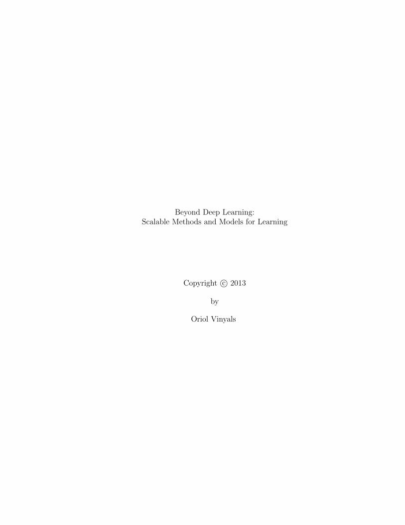
4.2.3 Experimental Results . . . . . . . . . . . . . . . . . . . . . . . . . . 40

5 Analysis – Why and how does depth matter? 46

5.1 Analysis – Regarding Layer Size . . . . . . . . . . . . . . . . . . . . . . . . 46

5.1.1 The Importance of Size . . . . . . . . . . . . . . . . . . . . . . . . . 46

5.1.2 Relationship Between Random Dictionaries and Nystrom Sampling . 48

5.1.3 Relationship between K′ and C′ . . . . . . . . . . . . . . . . . . . . 52

5.1.4 The metric in the coding space . . . . . . . . . . . . . . . . . . . . . 52

5.1.5 Dataset description . . . . . . . . . . . . . . . . . . . . . . . . . . . . 53

5.1.6 Pooling Aware Dictionary Learning . . . . . . . . . . . . . . . . . . . 54

5.1.7 Experiments . . . . . . . . . . . . . . . . . . . . . . . . . . . . . . . 58

5.2 Analysis – Regarding Depth . . . . . . . . . . . . . . . . . . . . . . . . . . . 60

5.2.1 Depth in Depth . . . . . . . . . . . . . . . . . . . . . . . . . . . . . . 60

5.2.2 Factors in Deep Learning . . . . . . . . . . . . . . . . . . . . . . . . 62

5.2.3 Experiments and Results . . . . . . . . . . . . . . . . . . . . . . . . 63

5.2.4 Depth in Vision . . . . . . . . . . . . . . . . . . . . . . . . . . . . . . 66

6 Keyword Spotting: A Speech Application 70

6.1 Keyword Spotting for Limited Resources . . . . . . . . . . . . . . . . . . . . 70

6.1.1 Limited Data and the BABEL Project . . . . . . . . . . . . . . . . . 70

6.1.2 The ICSI System and Babel . . . . . . . . . . . . . . . . . . . . . . . 71

6.1.3 The recognition system . . . . . . . . . . . . . . . . . . . . . . . . . 71

6.1.4 Discriminative Posting Refinements . . . . . . . . . . . . . . . . . . 73

6.1.5 Further Improvements of ATWV . . . . . . . . . . . . . . . . . . . . 77

6.2 Keyword Spotting for Unlimited Resources . . . . . . . . . . . . . . . . . . 78

iii

6.2.1 Computational Budget and Unlimited Data . . . . . . . . . . . . . . 78

6.2.2 Proposed Methods . . . . . . . . . . . . . . . . . . . . . . . . . . . . 78

6.2.3 Experiments . . . . . . . . . . . . . . . . . . . . . . . . . . . . . . . 81

7 Conclusions 85

7.1 Optimization . . . . . . . . . . . . . . . . . . . . . . . . . . . . . . . . . . . 85

7.2 Models . . . . . . . . . . . . . . . . . . . . . . . . . . . . . . . . . . . . . . . 86

7.3 Analysis . . . . . . . . . . . . . . . . . . . . . . . . . . . . . . . . . . . . . . 86

7.4 Applications . . . . . . . . . . . . . . . . . . . . . . . . . . . . . . . . . . . . 86

7.5 Concluding Remarks . . . . . . . . . . . . . . . . . . . . . . . . . . . . . . . 87

Bibliography 89

iv

Acknowledgements

Getting a PhD was more fun and interactive than I thought it would be when I first startedthinking about it during my undergrad at the Universitat Politecnica de Catalunya. Manypeople have helped me a lot in a day to day basis, and while pursuing my PhD I have beenlucky enough to find my life partner, Meire Fortunato. My parents, Jordi and Rosa, havealways been extremely helpful and supporting to everything I have done, and taught mefrom the principles of freedom that let me achieve such a big dream. My sister Georginahas always been there to give me a good laugh and her wonderful family sets a very highexample for me to try to follow. Many friends and special people have always been thereto share a drink and give me a laugh, and I want to specially thank Osito, Ruben, Carlos,Maria, Bea, Ivan, Marcos, Renato, Sebastian, Marcelo, Clarissa, Gabriel, Andrew, andmany others that I am forgetting right now!

I now come to realize how many amazing people I have worked and been lucky enough tolearn from during this years. A PhD is definitely not done in isolation! My advisor NelsonMorgan who, through his experience and points of view, has always given me good adviceand put me right in track to research towards this dissertation. Trevor Darrell, whomI consider a co-advisor, has been an extremely motivating source of knowledge in visionand learning, and has helped me broadening my skills beyond speech recognition. RuzenaBajcsy has also been an extremely kind and energetic person to work with, and BrunoOlshausen always had something more to say about current trends in machine learning,and his intuition and insights were extremely valuable and will help in the future.

At ICSI, I was able to collaborate with many postdocs, researchers, and students, sobig thanks to them all, specially Yangqing, Suman, Adam, Mary, Gerald, Kofi, Dan, Steve,Arlo, Korbinian, Chuck, Howard and Vijay, as well as all the staff members. Special thanksas well to Fernando from CMU for introducing me to research in the US, and to MSRfor supporting me through their Fellowship program that made my grad student life eveneasier.

Last but not least, through conferences and internships, I met a group of excellentresearchers. Thanks to Li Deng, Dan Povey, Dan Bohus, Geoff, Patrick, Jasha, Mike, Alex,Rich, Eric whom I met at MSR, and Vincent, Patrick (again!), Mike, Eric, Carolina, Andrewfrom Google. Also, kudos to George, James, Ilya, Alex, and Hinton from Toronto for themany useful discussions about deep learning.

v

Chapter 1

Introduction and Summary

In this thesis I present results from work that I hope will provide contributions to thespeech, vision, and machine learning communities. As a result of working in these differentareas, my thesis is interdisciplinary. The main emphasis is, however, common to all three:to learn something from data (or signal representations) with the objective of extractinguseful information. Learning is a very general word, so it is important to formalize exactlywhat it means in the context of machine learning and computer science. In Chapters 2,3 and 4, several parts of the learning process are carefully defined, but for the purpose ofthis introductory chapter, it is enough to think of learning as something that aims to find afunction that maps an input (e.g., a speech signal or an image) to an output (e.g., a wordspoken in a speech utterance, or an object class present in an image).

Thanks to increased computational power and data availability, machine learning iscontinuously evolving, and many algorithms and models are continuously revisited. Thistrend has been very clear in the beginning of the era of “Big Data”. As a result, somemethods that rely on large amounts of data are making a comeback. In particular, neuralnetworks, which are a powerful non-linear model to act as the function to map from inputsto outputs, have seen a renaissance. These models involve several layers of computation(typically with matrix-vector products and non-linearities). This is the main idea behind“Deep Learning”, which has been very popular amongst researchers and industry due toachieving state-of-the-art in many tasks and domains.

My main interests with regards to deep learning have been both in the learning itself(i.e., optimization), and the modeling part where, by trying to explore simpler optimizationproblems, one can achieve the same power in the function learned. My other main focushas been to apply these techniques to a wide variety of problems to show that, indeed, thesetechniques can generalize, with little to no tuning, to many learning tasks. However, thereis no magic, and every problem has singularities that require for us – the researchers – tofind the appropriate representation, model, and learning techniques that achieve the bestperformance.

My main contributions that are covered in this thesis have been:

• To optimization research by providing a robust and efficient second order method tooptimize functions (Chapter 3)

1

• To deep learning research, by proposing simple models that can be efficiently learned inparallel and have powerful representation power and regularization properties (Chap-ter 4)

• To deep learning research, by theoretically demonstrating why size matters and howdepth is important in learning (Chapter 5)

• To speech research, for advances in acoustic modeling by proposing new recurrentneural nets as a way to perform acoustic modeling, and for the analysis of variousacoustic models under different noise conditions (Chapter 6)

• Also to the speech research, for advances in keyword detection in both big data andscarcity of data (e.g., minority languages) conditions (Chapter 6), which resulted ina patent that is being used in millions of phones distributed in the latest GoogleAndroid Operating System

This thesis is organized in different chapters, which I summarize here. The reader isencouraged to read further in each chapter, which should be largely self contained (althoughsome references will be provided in lieu of a more complete explanation in some cases).

Chapter 2 explains current state of the art and puts in perspective each of the elementsof deep learning, emphasizing its success in applied fields such as speech recognition andcomputer vision. Although I leave some related work that is more specialized in its ownchapter, the object of Chapter 2 is to give a general overview of the state of the art.Furthermore, this chapter will define some of the jargon that will be used later in thethesis, which should help the reader unfamiliar with machine learning. This is intended toput in perspective the technical contributions that are presented in the following chapters.Readers that have experience with deep learning should jump ahead to chapters that reportthese contributions, as they also describe previous work on the field (though in a less generalway).

Chapter 3 proposes a new optimization algorithm specifically designed to train deeparchitectures, which are often challenging due to the non-convexity of the error surface andthe requirement to train such models with large amounts of data. Having these algorithmsnot only simplifies and speeds up the learning, but sometimes enables learning of modelsthat would be impossible with traditional methods. As such, this chapter also presentsrevisiting Recurrent Neural Networks (RNNs) for acoustic modeling as an application ofthe optimization algorithm.

In Chapter 4, even though optimizing challenging models is possible, I propose adeep learning architecture which would require the solution of several simpler (i.e., convex)problems instead of one big non-convex problem. Since there seems to be a trade offbetween model capacity and training difficulty, this chapter contrasts with Chapter 3 inthat it is trying to simplify the optimization algorithm while sacrificing as little modelcapacity as possible. Empirical evidence shows that this is, in general, possible with suchmodels, although I also point out some weaknesses and limitations of the simplified, easierto optimize model.

Given these observations, Chapter 5 changes focus from the methods and the mod-els, and tries to explain two fundamental characteristics that have made the current deeplearning “comeback” possible: first, I propose a theoretic framework to explain how size in

2

a single layer model relates to accuracy, and why there may be a need for depth. Secondly,I do an empirical study on how depth matters – although no theory is developed, the casestudy of a single layer network may help developing theory that solidifies our knowledge ondeep architectures versus shallow ones, which is currently an important open problem inthe machine learning community.

Chapter 6 presents several applications which show that, even though learning methodstry to be as general as possible, many tasks have singularities that need to be dealt with.There is no magic formula that solves every problem, thus implying that machine learningis an evolving research field, by no means solved, and that for some problems (includingsome presented in this chapter), deep learning is not well suited and other methodologiesshould be applied.

Chapter 7 concludes the thesis. This chapter aims to give a very personal and subjec-tive vision on what the future of machine learning may be, giving advice to future genera-tions working on deep learning and applied machine learning, and summarizing the contri-butions of this thesis, looking forward to the next decade doing applied machine learningresearch.

3

Chapter 2

Current Trends

2.1 Problem Statement and Definitions

The main focus of this thesis is the task of classification, which is a subfield of machinelearning (and which, itself, is as a subfield of artificial intelligence). Throughout the thesis Iwill refer to the classification task with other names such as supervised learning, or learning,but it should be clear what I am referring to given the context.

A classification function f takes inputs (usually called features) x, which typically livein the d-dimensional space Rd, and maps them to an output space. This output space mayrange from a one dimensional binary space (in which we want to classify whether an imagecontains a face or not), to the space of all English sentences (in which we are decodingan acoustic utterance into its transcription), or even real valued spaces (e.g., when we aretrying to predict the temperature given some observed variables from the weather). Thelatter is often called regression, but in this thesis I will make little distinction between thetwo.

Classification can can be thought of as a two stage process: the training (or learning)phase, and the testing (or inference). Almost all the efforts in this thesis concern the trainingphase, paying little to no attention to inference (other than computational considerationswhich will be clear in Chapters 4 and 6).

Although I go further in detail in Chapters 3 and 4, here I will briefly go over whatmachine learning entails. The goal is to “learn” a function f that maps an input x to anoutput y (both generally vectors, hence these symbols are bolded). This is a pretty vaguestatement, but the ingredients are all there already: f (the model), and pairs of x and y(the data). Fundamentally, we want to find a function that performs a classification taskwith human performance (sometimes, we can exceed human performance, but more oftenthan not, this is not the case). To achieve this, most of the approaches aim to maximize amerit function (or minimize a cost) on how well f performs given some data, and in somecases one could give a probabilistic interpretation to what is being learned (e.g. the meritfunction could be the likelihood when f is a probabilistic model).

One of the contributions of my thesis is the optimization algorithm which is used tomaximize the merit function, and is given in Chapter 3, while in Chapter 4 I focus onmethods to simplify f whilst keeping the maximization problem fairly straightforward (i.e.,

4

convex). This thesis also proposes novel applications of models to several classificationtasks, and the remainder of this chapter will focus on giving historical perspective to theproposed solutions to each of these tasks.

2.2 Optimization Techniques and Machine Learning

Many algorithms in machine learning and other scientific computing fields rely on opti-mizing a function with respect to a parameter space. In many cases, the objective functionbeing optimized takes the form of a sum over a large number of terms that can be treated asidentically distributed: for instance, labeled training samples. In deep learning, the problemoften consists of minimizing the negated log-likelihood:

f(θ) = − log(p(Y|X;θ)) = −N∑i=1

log(p(yi|xi;θ)) (2.1)

where (X,Y) are the observations and labels respectively (which are assumed independentand identically distributed), and p is the posterior probability of the labels which is modeledby a deep neural network with parameters θ. In this case it is possible to use subsets ofthe training data to obtain noisy estimates of quantities such as gradients; the canonicalexample of this is Stochastic Gradient Descent (SGD) [13].

My main interest is on batch methods (i.e., methods that process the whole sum, ora large portion of the sum in equation 2.1), as they are easy to parallelize across severalmachines [34], which is often desirable in language and speech as we typically have millionsof training examples. However, some methods have been studied where a powerful sin-gle computational device (such as a Graphical Processing Unit (GPU)) is used to quicklycompute a small subset of the sum, and updates the model very frequently (but not asaccurately as one would with batch methods), leading to stochastic or mini-batch methods[13], which can outperform batch method in terms of compute time to convergence. Thesemethods are hard to parallelize because their main characteristic is very frequent updates ofthe parameters, which requires low latency and large memory bandwidth. Besides the dis-cussion of batch versus mini-batch (or stochastic) methods in terms of accuracy of gradientsversus more frequent model updates, a chief advantage of batch methods is that we can addsecond order information. In practice, some mini-batch methods have shown improvementswhen using curvature [42], but in general best results are obtained when considering batchmethods due to having no noise in the estimation of our objective function.

The simplest reference point to start from when explaining second order methods isNewton’s method with line search, where on iteration m we do an update of the form:

θm+1 = θm − αH−1m gm, (2.2)

where Hm and gm are, respectively, the Hessian and the gradient on iteration m of theobjective function (2.1); here, α would be chosen to minimize (2.1) at θm+1. For highdimensional problems it is not practical to invert the Hessian; however, we can efficientlyapproximate (2.2) using only multiplication by Hm, by using the Conjugate Gradients (CG)method with a truncated number of iterations. In addition, it is possible to multiply byHm without explicitly forming it, using what is known as the “Pearlmutter trick” [103] for

5

multiplying an arbitrary vector by the Hessian (the algorithm is described in Chapter 3);this is described for neural networks but is applicable to quite general types of functions1.This type of optimization method is known as “truncated Newton” or “Hessian-free inexactNewton” [89]. In [20], this method is applied but using only a subset of data to approximatethe Hessian Hm. A more sophisticated version of the same idea was described in the earlierpaper [82], in which preconditioning is applied, the Hessian is damped with the unit matrixin a Levenberg-Marquardt fashion, and the method is extended to non-convex problemsby using the Gauss-Newton matrix (described in Chapter 3) as a substitute the Hessian.These changes made it possible to use HF to effectively train deep networks from randominitializations, which would not have been possible with any previously described versionsof HF.

2.3 Neural Networks and Deep Learning

A Neural Network (NN) in the context of machine learning and computer science refersto an artificial neural network, but it was back in 1943 when McCulloch and Pitts – aneurophysiologist and a mathematician – presented results on how neurons may work andmodeled a neural network using circuits. In the late 50s and early 60s, Widrow at Stanfordsuccessfully applied neural networks to solve a real problem (related to speech processing inphone lines). Neural Networks are sometimes referred as Multi Layer Perceptrons (MLP),which are related to the perceptron algorithm introduced in 1957 [113], and which can beseen as a neural network without hidden units. It is out of the scope of this their to reviewthe history of neural networks, but the enthusiast reader is encouraged to read [111]. Alot of work has been done in neural networks for acoustic modeling, and further details aregiven in the following section.

Leaping forward in time, neural networks are back in fashion with the somewhat hypedterm “Deep Learning”, which rose from the 2006 work of Hinton [58]. One of the mainproperties of deep learning (or deep architectures) is to compose (or stack) several layers ofcomputation (deep typically refers to having many “hidden” layers). In [137], the conceptof stacking was proposed where simple modules of functions or classifiers are “stacked” ontop of each other in order to learn complex functions or classifiers. Since then, variousways of implementing stacking operations have been developed, which can be categorizedas unsupervised and supervised approaches.

Unsupervised approaches perform stacking in a layer-by-layer fashion that typicallyinvolves no label information. This gives rise to multiple layers in unsupervised featurelearning, as exemplified in Deep Belief Networks [59, 57], layered Convolutional NeuralNetworks [63], Deep Auto-encoder [59, 37], etc. Applications of such stacking methodsincludes object recognition [63, 27], speech recognition [88], etc.

Supervised approaches, which are closer to the focus of this thesis, carry out stackingwith the help of labels in the learning of each layer, which is typically a simple classifier.The new features for the stacked classifier at a higher level of the hierarchy come from com-bination of the classifier output of lower modules and the raw input features. Cohen and deCarvalho [28] developed a stacking architecture where the simple module is a ConditionalRandom Field. Another successful stacking architecture reported in [38] uses supervised

1This was actually known to the optimization community prior to [103]; see [97, Chapter 8] and [53].

6

information for stacking where the basic module is a simplified form of multilayer percep-tron where the output units are linear and the hidden units are sigmoidal nonlinear. Thelinearity in the output units permits highly efficient, closed-form estimation (results of con-vex optimization) of the output network weights given the hidden units’ outputs. Stackedcontext has also been used in [14], where a set of classifier scores are stacked to produce amore reliable detection. The proposed method in Chapter 4 will build a stacked architecturewhere each layer is a linear SVM, which has proven to be a successful classifier for manyapplications.

One of the challenges with the MLP and the DNN is that the objective function isnon-convex, and as more hidden layers are added, finding a good local minima becomesmore challenging. Motivated by this problem, DNNs with pretraining based on RestrictedBoltzman Machines, denoted as Deep Belief Networks (DBNs), were introduced in [58] andhave been applied to several fields such as computer vision (see [59]), phone classification(see [86]), speech recognition [133, 88, 119, 31], and speech coding (see [37]). The new ideais to train each layer independently in a greedy fashion, by sequentially using the hiddenvariables as observed variables to train each layer of the deep structure. Recently, the useof DNNs with no pretraining has also been studied [31, 119].

2.4 Speech Recognition, Acoustic Modeling, and KeywordDetection

Speech Recognition and Acoustic Modeling

The main focus of this thesis with regards to speech processing is acoustic modelingand keyword spotting. Acoustic modeling aims to predict a phonetic unit (a monophone,triphone state, or similar) from a segment of audio. This (generally probabilistic) modelis then used in many current systems in a Hidden Markov Model (HMM) as the emissionprobability model, in which the hidden state (typically a triphone state) emits the obser-vation (speech signal). HMM is a powerful statistical sequence model that was proposedin [7] and first introduced in speech recognition independently by [5] and [4]. Adding aLanguage Model (LM) one can decode a speech signal to its most likely sentence. A non-expert reader that has interest in the whole speech recognition pipeline is encouraged toread further details in one of the many references that exist in this topic (e.g. [50]).

Acoustic modeling is one of the key components in the performance of a speech recogni-tion system. The most common trend up to the explosion of deep learning research focusedon using Mel Frequency Cepstral Coefficients (MFCC) as features to train a Gaussian Mix-ture Model (GMM). Using features other than MFCCs has long been a focus of researchin the speech recognition community, and the combination of various feature streams hasproven useful in a variety of speech recognition systems. A common technique to mergestreams is to use a Tandem method [54], in which processed phone posterior probabilitiesare appended to standard MFCCs.

As noted above, neural networks have been used for speech recognition for some time; infact, there were early experiments at Stanford by B. Widrow and his students in the 1960s[124]. In the 1980s, a number of laboratories in Europe, the U.S, and Japan revived workon using neural networks to classify speech categories, and ultimately to generate speech

7

category probabilities for use with hidden Markov models, which by then were the dominantmethod for dealing with the sequence of sounds in speech. In general these networks used asingle hidden layer and a modest number of categories, although as noted above there werenotable exceptions. For example, the HNN/ACID approach of J. Fritsch [47] used a tree ofnetworks in order to estimate a large number of context-dependent classes, using the simplefactoring trick expounded in [90]. Input to the Fritsch system was processed by a number ofnetworks in order to derive probability estimates at the leaves, and thus was an example ofan extremely deep network that was also context-dependent. It performed quite well on anumber of large vocabulary tasks at the time. This network and many others were examplesof the hybrid HMM/MLP approach [91]. However, by 2000 it had become quite difficult forsuch systems to keep up competitively with the plethora of engineering advances that weredeveloped for HMM/GMM systems, given the huge number of excellent laboratories thatfocused on improving the latter. The turning point for some of us was the Aurora task, inwhich we were required to use an HMM/GMM system with fixed characteristics and onlycould modify the front end. And so the Tandem approach [54] was adopted by many ofus, in which the same networks we had developed were now used to generate features foran HMM/GMM system. This permitted researchers to continue to develop neural networkapproaches while taking advantage of advances in HMM/GMM systems.

Using these approaches, other systems were developed in which networks trained for anintermediate goal were then incorporated in larger networks, resulting in a deep structure;for example, a hierarchical system focused on temporal modulations of the spectrum [55]and systems that trained networks to focus on temporal characteristics within each criticalband and then combined these networks with another network, e.g., [24]. Thus, manyexperiments were done in which some input variables (e.g., MFCC or mel spectra) wereprocessed by multiple layers of artificial neurons prior to use by an HMM of some form.However, all of these techniques were largely relegated to providing an assist to a largerHMM/GMM system prior to the recent revival of hybrid HMM/MLP systems that has goneunder the name of “deep neural networks” of various kinds.

One of the problems with MLPs is that the objective function is non-convex, and asmore hidden layers are added, finding a good local minimum becomes more challenging.Motivated by this problem, Deep Belief Networks were introduced in [59] and have beenapplied in several fields such as computer vision (see [59]), phone classification (see [86, 88]),and speech coding (see [37]). The new idea is to train each layer independently in a greedyfashion, by sequentially using the hidden variables as observed variables to train each layerof the deep structure.

Initial success using DBNs on fairly small datasets and using small models quicklyevolved, and the positive results of having deep models that yielded state-of-the-art acousticmodeling was adopted and generalized in many tasks and with much larger models [31, 119,62, 57]. In the following paragraphs, I discuss previous work that focuses on the analysis andunderstanding of why neural networks have seen such a renaissance for acoustic modeling.

Since in this thesis I attempt to explain, in a limited context, the main contributingfactors that make deep learning successful are, I next review some of the previous work thatdiscussed such key points in chronological order.

In [31], many interesting points were raised. First, in a large system such as the one thatwas used there (with 2000 hours), having triphone units as targets instead of monophones

8

(which were more commonly use in previous work, with exceptions, as noted above) mayhave been the main contributing factor to the results obtained (4% absolute gains). Addinglayers generally resulted in better accuracy, but the number of parameters was increasedwith every layer added, so that it was not entirely clear what was the main contributingfactor to the good results - the depth, or the larger number of parameters. However, aflat (or shallow) model having the same parameters as the deepest model was also trained,which was 2% worse than the deep model. Additionally, pretraining added 2% in accuracy.

In [119], another method for pretraining was used, and again the depth of the modelwas demonstrated to be one of the key contributions to the 30% relative improvement. Animportant contribution in that work was the effect of pretraining. For smaller tasks such asTIMIT or MNIST, pretraining was found important as, besides helping the optimization ofa deep architecture, provided a form of regularization to the network by using unsupervisedlearning. In the work by Seide et al, the architecture rather than pretraining seemed to bemore important, and other forms of pretraining such as discriminative pretraining was ableto perform as well as RBM pretraining.

Recent work in [35, 87] analyzed the input to the networks, and showed that log filterbanks may be a better input instead of other transformations (e.g., MFCC), which havebeen the mainstream feature in classical GMMs due to some assumptions such as diagonalcovariance.

Keyword Detection

Although heavily related to speech recognition, keyword spotting (or detection) is simi-lar to the object recognition task in computer vision, where given a signal (image or speechutterance), the goal is to predict if a given object is present in it (this could be a chair in aimage, or the word “capital” in an utterance). Besides detecting if a word is present, we canalso predict the location of that word (similarly for an object in an image). The researchon keyword spotting has paralleled the development of the Automatic Speech Recognition(ASR) domain in the last years. Like ASR, keyword spotting has first been addressedwith models based on Dynamic Time Warping (DTW) [19, 56]. Then, approaches basedon discrete HMMs were introduced [67]. Finally, discrete HMMs have been replaced bycontinuous HMMs [108]. There have been many attempts to do discriminative training,but the most relevant one is [51], which targets a figure of merit instead of the error rate,and which is the baseline that I used in Section 6.2.

2.5 Computer Vision and Object Classification

There has been a trend in object, acoustic and image classification to move the com-plexity from the classifier to the feature extraction step. The main focus of many stateof the art systems has been to build rich feature descriptors (e.g., SIFT [79], HOG [32] orMFCC [33]), and use sophisticated non-linear classifiers, usually based on kernel functionsand SVM or mixture models. Thus, the complexity of the overall system (feature extrac-tor followed by the non-linear classifier) is shared in the two blocks. Vector Quantization[44], and Sparse Coding [100, 139, 142] have theoretically and empirically been shown towork well with linear classifiers. In [27], the authors note that the choice of codebook doesnot seem to impact performance significantly, and encoding via an inner product plus a

9

non-linearity can effectively replace sparse coding, making testing significantly simpler andfaster.

A disturbing issue with sparse coding + linear classification is that with a limitedcodebook size, linear separability might be an overly strong statement, undermining the useof a single linear classifier. This has been empirically verified: as we increase the codebooksize, the performance keeps improving [27], indicating that such representations may notbe able to fully exploit the complexity of the data [12]. In fact, recent success on PASCALVOC could partially be attributed to a huge codebook [140]. While this is theoreticallyvalid, the practical advantage of linear models diminishes quickly, as the computation costof feature generation, as well as training a high-dimensional classifier (despite linear), canmake it as expensive as classical non-linear classifiers.

Despite this trend to rely on linear classifiers and overcomplete feature representations,sparse coding is still a flat model, and efforts have been made to add flexibility to thefeatures. In particular, Deep Coding Networks [78] proposed an extension where a higherorder Taylor approximation of the non-linear classification function is used, which showsimprovements over coding that uses one layer. My approach can be seen as an extension tosparse coding used in a stacked architecture.

I illustrate the feature extraction pipeline that is composed of encoding dense localpatches and pooling encoded features later in this thesis in Figure 5.1, and provide a briefreview here. This pipeline is architecturally very similar to Convolutional Neural Networks(see [76, 73]), but instead relies on unsupervised learning (rather than fine tuning) of thenetwork parameters. Specifically, starting with an input image I, I formally define theencoding and pooling stages as follows.

(1) Coding. In the coding step, one extracts local image patches2, and encode each patchto c activation values based on a dictionary of size c (learned via a separate dictionarylearning step). These activations are typically binary (in the case of vector quantization)or continuous (in the case of e.g., sparse coding), and it is generally believed that havingan over-complete (c > the dimension of patches) dictionary while keeping the activationssparse helps classification, especially when linear classifiers are used in the later steps.

I will mainly focus on the decoupled encoding methods, in which the activation of onecode does not rely on other codes, such as threshold encoding [27], which computes theinner product between a local patch x and each code, with a fixed threshold parameterα: c(x) = max{0,x>D − α} where D ∈ Rd×c is the dictionary. Such methods have beenincreasingly popular mainly for their efficiency over coupled encoding methods such assparse coding, for which a joint optimization needs to be carried out. Their employment inseveral deep models (e.g., [73]) also suggests that such a simple non-linearity may suffice tolearn a good classifier in the later stages.

(2) Learning the dictionary: Recently, it has been found that relatively simple dictio-nary learning and encoding approaches lead to surprisingly good performances [26, 117].For example, to learn a dictionary D = [d1,d2, · · · ,dc] of size K from a set of local patches

2Although I use the term “patches” throughout the thesis, the pipeline works with local image descriptors,such as SIFT, as well.

10

X = {x1,x2, · · · ,xN} each reshaped as a vector of pixel values, one could simply adopt theK-means algorithm, which aims to minimize the squared distance between each patch andits nearest code: minD

∑Ni=1 minj ‖xi−dj‖22. I refer to [26] for a detailed comparison about

different dictionary learning and encoding algorithms.

(3) Pooling. Since the coding result are highly over-complete and highly redundant, thepooling layer aggregates the activations over a spatial region of the image to obtain a cdimensional vector, where each dimension of the pooled feature is obtained by taking theoutput of the corresponding code in the given spatial region (also called receptive field inthe literature) and performing a predefined operator (usually average or max). Figure 5.1shows an example when average pooling is carried out over the whole image. In practice onemay define multiple spatial regions per image (such as a regular grid or a spatial pyramid),and the global representation for the image will then be a vector of size c times the numberof spatial regions.

11

Chapter 3

Optimization Challenges inLearning

Part of the work that appears on this chapter has been published in peer reviewedconferences. The optimization algorithm was presented at NIPS 2011 an AISTATS 2012[132], and the Recurrent Neural Network work was presented at ICASSP 2012 [134].

The main challenges in optimizing

f(θ) = − log(p(Y|X;θ)) = −N∑i=1

log(p(yi|xi;θ)) (3.1)

are as follows:

• θ can be very high dimensional

• Y and X could be very large (both in dimensionality and in number of trainingsamples)

• The function to optimize f (or, equivalently, the model p) can be expensive to compute

• The objective function to optimize can be non-convex and ill-conditioned

As a result, I propose a new algorithm which I call Krylov Subspace Descent (KSD)which partially copes with the above issues by:

• Never storing more than a few copies of the parameter θ, whilst achieving secondorder convergence rates

• Using large batches and accurate updates of parameters, thus being able to efficientlyuse compute clusters

• Using curvature information, which tremendously helps some problems which are ill-conditioned (near zero curvature)

• Being mostly hyperparameter free, thus being applicable to a large number of models,merit functions, and problem scales (the same parameter settings have been used formany different models, datasets, and scales)

12

My method is quite similar to the one described in [82], which I will refer to as HessianFree (HF). I also multiply by the Hessian (that is, the matrix of second derivatives w.r.t.the parameters) using the Pearlmutter trick on a subset of data. The Pearlmutter trickcomputes the product of H times a vector without explicitly storing the matrix, at thecost of a forward and backward pass through the neural network, hence the name “HessianFree” (see Algorithm 1 for more details). The chief difference between KSD and HF is that,in each iteration, instead of approximately computing (Hm + λI)−1gm using truncatedConjugate Gradient (CG), I compute a basis for the Krylov subspace of dimension K whichis defined by the span of gm,Hmgm, . . .H

K−1m gm for some K fixed in advance (e.g., K = 20),

and numerically optimize the parameter change within this subspace, using BFGS1 [96] tominimize the original nonlinear objective function measured on a subset of the trainingdata. It is easy to show that, for any λ, the approximate solution to Hm + λI found byK iterations of CG will lie in this subspace, so I am in effect automatically choosing theoptimal λ in the Levenburg-Marquardt smoothing method of HF – although the algorithmis free to choose a solution more general than this. This is clear from the CG algorithmitself, and from the fact that the order-K Krylov subspaces generated by g and H + λIare all the same irrespective of λ. Note that both my method and HF use preconditioning,which I have glossed over in the discussion above. Compared with HF, the advantages ofmy method are:

• Greater simplicity and robustness: there is no need for heuristics to initialize andupdate the smoothing value λ.

• Generality: unlike HF, my method can be applied even if H (or whatever approxima-tion or substitute used) is not positive semidefinite.

• Empirical advantages: my method generally seems to work better than HF in bothoptimization speed and classification performance.

The chief disadvantages versus HF are:

• Memory requirement: it requires storage of K times the parameter dimension tostore the subspace (HF does not require memory proportional to the number of CGiterations).

• Convergence properties: the use of a subset of data to optimize over the subspace willprevent convergence to an optimum.

Regarding the convergence properties: for deep neural networks, this is more of a the-oretical than a practical problem, since for typical setups in training deep networks theresidual parameter noise due to the use of data subsets would be far less than that dueto overtraining. One would hope that not-too-restrictive conditions could be found underwhich the algorithm (or a modified version of it, with increasing subset sizes) could beshown to converge; however, I do not have either the time or the skills needed to performthis type of analysis by myself. I also believe that application of the normal types of con-vergence proof would fail to capture the reasons why the algorithm is better than gradient

1BFGS (named after its inventors) is a second order method that uses a low rank approximation of theHessian matrix so that it can be efficiently inverted thanks to the Matrix Inversion Lemma.

13

descent, and it would be very hard to obtain convergence results that were strong enoughto be interesting. However, empirical evidence suggests that convergence to a local minimais faster using methods such as KSD or HF than with vanilla SGD.

My motivation for the work presented here is twofold: firstly, I am interested in large-scale non-convex optimization problems where the parameter dimension and the number oftraining samples is large and the Hessian has a large condition number. I have previouslyinvestigated quite different approaches based on preconditioned Stochastic Gradient Descent(SGD) to solve an instance of this type of optimization problem (my method could be viewedas an extension to [114]), but after reading [82] my interest switched to methods of the HFtype. Secondly, I have an interest in deep neural nets, particularly to solve problems inspeech recognition, and I was intrigued by the suggestion in [82] that the use of optimizationmethods of this type might remove the necessity for pretraining, which would result in awelcome simplification. Other recent work on the utility of second order methods for deepneural networks includes [9] and [75].

3.1 The Hessian matrix and the Gauss-Newton matrix

The Hessian matrix H can be used implicitly in HF optimization whenever it is guaran-teed positive semidefinite, i.e., when minimizing functions that are convex in the parameters.For non-convex problems, it is possible to substitute a positive definite approximation tothe Hessian. One option is the Fisher information matrix,

F =∑i

gigTi , (3.2)

where indices i correspond to samples and the gi quantities are the gradients for each sample.This is a suitable stand-in for the Hessian because it is in a certain sense dimensionally thesame, i.e. it changes the same way under transformations of the parameter space. Ifthe model can be interpreted as producing a probability or likelihood, it is possible undercertain assumptions (including model correctness) to show that close to convergence, theFisher and Hessian matrices have the same expected value. The use of the Fisher matrix inthis way is known as Natural Gradient Descent [3]; in [114], a low-rank approximation of theFisher matrix was used instead. Another alternative that has less theoretical justificationbut which seems to work better in practice in the case of neural networks is the Gauss-Newton matrix, or rather a slight generalization of the Gauss-Newton matrix that we willnow describe.

3.1.1 The Gauss-Newton matrix

The Gauss-Newton matrix is defined when we have a function (typically nonlinear) froma vector to a vector, f : Rn → Rm. Let the Jacobian of this function be J ∈ Rm×n, thenthe Gauss-Newton matrix is G = JTJ, with G ∈ Rn×n. If the problem is least-squareson the output of f , then G can be thought of as one term in the Hessian on the input tof . In its application to neural-network training, for each training example I consider thenetwork as a nonlinear function from the neural-network parameters θ to the output ofthe network, with the neural-network input treated as a constant. As in [118], I generalize

14

this from least squares to general convex error functions by using the expression JTHJ,where H is the (positive semidefinite) second derivative of the error function w.r.t. theneural network output. This can be thought of as the part of the Hessian that remainsafter ignoring the nonlinearity of the neural-network in the parameters. In the rest of thisdocument, following [82] I will refer to this matrix JTHJ simply as the Gauss-Newtonmatrix, or G, and depending on the context, I may actually be referring to the summationof this expression over a number of neural-network training samples.

3.1.2 Efficiently multiplying by the Gauss-Newton matrix

As described in [118], it is possible to efficiently multiply a vector by G using a version ofthe “Pearlmutter trick”; the algorithm is similar in spirit to backprop and for completenessI give it here as Algorithm 1; however, the reader should feel free to skip over this sectionif this level of detail is not required.

My notation and my derivation for this algorithm differ from [103, 118], and I willexplain this briefly with the hope that my explanation is easier to follow. The basic idea isto write down an algorithm that efficiently computes the inner product of the Gauss-Newtonmatrix with two given vectors (i.e. s = θT2 Gθ1), and then use reverse-mode automaticdifferentiation (similar to neural-net backprop) to compute the derivative of this scalarw.r.t. θ2, which will equal the desired product Gθ1.

First I will explain how I compute the inner product. Imagine that we are given aparameter vector θ, and two vectors θ1 and θ2 which we interpret as directions in parameterspace; we want to write down an algorithm that computes the scalar s = θT2 Gθ1. Assumethe neural-network input is given and fixed; let v be the network output, and write it asv(θ) to emphasize the dependence on the parameters, and then let v1 be defined as

v1 = limα→0

1

α(v(θ + αθ1)− v(θ)) , (3.3)

so that v1 = Jθ1. I define v2 similarly. These can both be computed in a modified forwardpass through the network, using forward-mode automatic differentiation. Then, if HE isthe Hessian of the error function in the output of the network (taken at parameter valueθ), s is given by

s = vT2 HEv1, (3.4)

since vT2 HEv1 = θT2 JTHEJθ1 = θT2 Gθ1. The Hessian HE of the error function wouldtypically not be constructed as a matrix, but we would compute (3.4) given some analyticexpression for H. This Hessian HE w.r.t. the output activations for a particular sampleshould not be confused with the Hessian w.r.t. the parameter vector. Suppose we havewritten down the algorithm for computing s (I have not done so here because of spaceconstraints). Then we treat θ1 as a fixed quantity, but compute the derivative of s w.r.t.θ2, taking θ2 around zero for convenience. This derivative equals the desired product Gθ1.This is how I obtained Algorithm 1. In the algorithm I denote the derivative of s w.r.t.a quantity x by x, i.e. by adding a hat. Note that in this algorithm, I have a “backwardpass” for quantities with subscript 2, which did not appear in the forward pass, becausethey were zero (since we take θ2 = 0) and I optimized them out.

Something to note here is that when the linearity of the last layer is softmax and theerror is negated cross-entropy (equivalently negated log-likelihood, if the label is known),

15

I actually view the softmax nonlinearity as part of the error function. This is a closerapproximation to the Hessian, and the error function remains positive semidefinite.

To explain the notation of Algorithm 1: h(i) is the input to the nonlinearity of thei’th layer and v(i) is the output; � means elementwise multiplication; φ(i) is the nonlinearfunction of the i’th layer, and when we apply it to vectors it acts elementwise; W(1) isthe matrix of neural-network weights for the first layer (so h(1) = W(1)v(0), and so on); Iuse the subscript 1 for quantities that represent how quantities change when we move theparameters in direction θ1 (as in Eq. (3.3)). The error function is written as E(v(L), y)(where L is the last layer), and y, which may be a discrete value, a scalar or a vector,represents the supervision information which the network is trained with. Typically Ewould represent a squared loss or negated cross-entropy. In the squared-loss case, thequantity ∂2

∂v2E(v(L), y) in Line 10 of Algorithm 1 is just the unit matrix. The other caseI deal with here is negated cross entropy. I include the soft-max nonlinearity in the errorfunction, treating the elements of the output layer v(L) as unnormalized log probabilities.If the elements of v(L) are written as vj and we let p be the vector of probabilities, withpj = exp(vj)/

∑i exp(vi), then the matrix HE of second derivatives is given by

∂2

∂v2E(v(L), y) = diag(p)− ppT . (3.5)

Algorithm 1 Compute product θ2 = Gθ1: MultiplyG(θ,θ1,x, y)

1: // Note, θ = (W(1),W(2), . . .) and θ1 = (W(1)1 ,W

(2)2 , . . .).

2: v(0) ← x3: v

(0)1 ← 0

4: for l = 1 . . . L do5: h(l) ←W(l)v(l−1)

6: h(l)1 ←W(l)v

(l−1)1 + W

(l)1 v(l−1)

7: v(l) ← φ(l)(h(l))

8: v(l)1 ← φ′(l)(h(l))� h

(l)1

9: end for10: v

(L)2 ← ∂2

∂v2E(v(L), y)v(L)1

11: for l = L . . . 1 do12: h

(l)2 ← v

(l)2 � φ′(l)(h(l))

13: v(l−1)2 ← W(l) T h

(l)2

14: W(l)2 ← h

(l)2 v(l−1) T

15: end for16: return θ2 ≡

(W

(1)2 , . . . ,W

(L)2

)

3.2 Krylov Subspace Descent: overview

Now I describe the method, and how it relates to Hessian Free (HF) optimization.The discussion in the previous section (on the Hessian versus Gauss-Newton matrix) isorthogonal to the distinction between KSD and HF, because either method can use anyHessian substitute, with the proviso that my method can use the Hessian even when it isnot positive definite.

16

In the rest of this section I will use H to refer to either the Hessian or a substitute suchas G or F. In [82] and in the work I describe here, these matrices are approximated usinga subset of data samples. In both HF and KSD, the whole computation is preconditionedusing the diagonal of the Fisher matrix F (since this is easy to compute, although otherapproaches have been recently proposed [23]); however, in this overview I will gloss overthis preconditioning. In HF, on each iteration the CG algorithm is used to approximatelycompute

d = −(H + λI)−1g, (3.6)

where d is the step direction, and g is the gradient. As described in [82], CG aims tominimize the function 1

2xT (H + λI)x − xTg which is a quadratic approximation of theobjective function. The approximate solution dCG reached after K iterations of CG willlie in the Krylov subspace of dimension K which is, by definition, the subspace spanned by{g, (H + λI)g, . . . , (H + λI)K−1g}. This is easy to see by looking at the CG algorithm.

In HF, the step size to take in the direction dCG is determined by a backtracking linesearch. The value of λ is kept updated by Levenburg-Marquardt style heuristics. Otherheuristics are used to control the stopping of the CG iterations. In addition, the CGiterations for optimizing d are not initialized from zero (which would be the natural choice)but from the previous value of d; this loses some convergence guarantees but seems toimprove performance, perhaps by adding a kind of momentum to the updates.

In my method, I compute an orthogonal basis P for the subspace spanned by{g,Hg, . . . ,HK−1g,dprev}, which is the Krylov subspace of dimension K generated byg and H, augmented with the previous search direction. Note that the Krylov subspaceof dimension K generated by g and H + λI is the same as that generated by g and H,which is easy to verify. The method optimizes the objective function f over this subspaceusing BFGS, approximating the objective function using a subset of samples. The BFGSphase may be viewed as a modification of the line search phase of HF, but done in a higherdimension and using a subset of the data. The BFGS phase uses a different subset of datafrom that used to compute the Hessian; if I used the same subset I would get a very biasedestimate of the optimal step to take within the subspace.

The complete algorithm is given as Algorithm 2. The most important parameter is K,the dimension of the Krylov subspace (e.g. 20). The flooring constant ε is an unimportantparameter; I used 10−4. The subset sizes may be important; I recommend that An shouldbe all of the training data, and Bn and Cn should each be about 1/K of the training data,and disjoint from each other but not from An. This is the subset size that keeps the com-putation approximately balanced between the gradient computation, subspace constructionand subspace optimization. Implementations of the BFGS algorithm would typically alsohave parameters: for instance, parameters of the line-search algorithm and stopping crite-ria; however, I expect that in practice these would not have too much effect on performancebecause the algorithm is likely to converge almost exactly (since the subspace dimensionand the number of iterations are about the same).

Each iteration of Algorithm 2 computes a Krylov subspace of dimension K from thegradient and the Hessian or Hessian substitute, and optimizes over this subspace usingBFGS with the objective function approximated using a data subset Cn. Lines 7 to 9 are anadditional preconditioning step to help the BFGS to converge faster, in which I try to findnew co-ordinates in which H is the unit matrix. Line 7 is needed to handle cases where H

17

Algorithm 2 Krylov Subspace Descent

1: dprev ← e1 // or any arbitrary nonzero vector

2: for n = 1, 2 . . . do3: // Sample three sets from training data, An, Bn and Cn.

4: g← 1|An|

∑i∈An

gi(θ) // Get average function gradient over this batch.

5: Set D to diagonal of Fisher matrix on An, floored to ε times its maximum.6: Find P and H on subset Bn (algorithm omitted)7: Let H be the result of flooring the eigenvalues of H to ε times the maximum.8: Do the Cholesky decomposition H = CCT

9: Let P = PC−T (do this in-place; C−T is upper triangular)10: a← 0 ∈ RK+1

11: Find the value a∗ that minimizes the objective function measured on Cn, using aboutK iterations of BFGS, with objective function measured at θ+ Pa and gradient PTg(where g is the gradient w.r.t. the parameters, measured at parameter-value θ+Pa).

12: dprev ← Pa∗

13: θ ← θ + dprev

14: end for

Dataset #Train #Test Input Output Model Task

CURVES 20K 10K 784 (bin.) 784 (bin.) 400-200-100-50-25-5 AEMNISTAE 60K 10K 784 (bin.) 784 (bin.) 1000-500-250-30 AEMNISTCL 60K 10K 784 (bin.) 10 (class) 500-500-2000 ClassMNISTCL,PT

1 60K 10K 784 (bin.) 10 (class) 500-500-2000 ClassAurora 1.2M 100K2 352 (real) 56 (class) 512-1024-1536 ClassStarcraft 900 100 5077 (mix) 8 (class) 10 Class

Table 3.1. Datasets and models used in my setup.

has zero or negative eigenvalues. The flooring described in Line 7 may be done as follows:do the Singular Value Decomposition H = UDVT , then let D be a floored version of D,with diagonal elements di = max(di, εmaxi di); then let H = UDUT (note: the use of Uon both sides is not a typo). This has the effect of flipping the sign of negative eigenvalues,and then imposing a floor of ε times the largest eigenvalue.

3.3 Experiments

To evaluate KSD, I performed several experiments to compare it with SGD and withother second order optimization methods2, namely L-BFGS and HF. I report both trainingand cross validation errors, and running time (I terminated the algorithms with an earlystopping rule using held-out validation data). My implementations of both KSD and HFare based on Matlab using Jacket3 to perform the expensive matrix operations on a GeforceGTX580 GPU with 1.5GB of memory.

2Note: I may properly speak of HF and KGD as second-order methods only when H is the actual Hessianmatrix

3www.accelereyes.com

18

2.7 2.9 3.1 3.3 3.5 3.7

0.2

0.4

0.6

log10

(time(s))

Tra

in E

rror

HF, Hessian matrixLBFGSHF, GN matrixKSD, Hessian matrixKSD, GN matrix

2.4 2.6 2.8 3 3.2 3.40

4

8

12

16

18

log10

(time(s))

L 2 Tra

in E

rror

LBFGS

HF, Hessian matrix

KSD, GN matix, K=80

KSD, Hessian matrix, K=20

HF, GN matrix

KSD, GN matrix, K=20

Figure 3.1. Aurora and CURVES convergence curves for various algorithms.

3.3.1 Datasets and models

Here I describe the datasets that I used to compare KSD to other methods.

• CURVES: Artificial dataset consisting of curves at 28×28 resolution. The dataset con-sists of 20K training samples, and 10K testing samples. I considered an autoencodernetwork, as in [59].

• MNIST: Single digit vision classification task. The digits are 28 × 28 pixels, with a60K training, and 10K testing samples. I considered both an autoencoder network,and classification [59].

• Aurora: Spoken digits dataset, with different levels of real noise (airport, train station,...). I used Perceptual Linear Prediction features and performed classification of 56English phones. These frame level phone error rates are the ones reported in Table 3.2.Also reported in the text are Word Error Rates, which were produced by using thephone posteriors in a Tandem system, concatenated with standard MFCC to train aHidden Markov Model with Gaussian Mixture Model emissions. Further details onthe setup can be found in [133].

• Starcraft: The dataset consists of a real time strategy video game sequences from1000 games. The goal is to predict the strategy the opponent chose based on a fullyobserved game sequence after five minutes, and features contain orderings betweenbuildings, presence/absence features, or times that certain buildings were built.

The models (i.e. network architectures) for each dataset are summarized in Table 3.1.I tried to explore a wide variety of models covering different sizes, input and output char-acteristics, and tasks. Note that the error reported for the autoencoder (AE) task is the L2norm squared between input and output, and for the classification (Class) task is the clas-sification error (i.e. 100 - accuracy). The non linearities considered were logistic functionsfor all the hidden layers except for the “coding” layer (i.e. middle layer) in the autencoders,which was linear, and the visible layer for classification, which was softmax.

1For MNISTCL,PT I initialize the weights using pretraining RBMs as in [59]. In the other experiments,I did not find a significant difference between pretraining and random initialization as in [82].

2I report both classification error rate on a 100K CV set, and word error rate on a 5M testing set withdifferent levels of noise

19

HF KSD

Dataset Tr. err. CV err. Time Tr. err. CV err. Time

CURVES 0.13 0.19 1 0.17 0.25 0.2MNISTAE 1.7 2.7 1 1.8 2.5 0.2MNISTCL 0% 2.01% 1 0% 1.70% 0.6MNISTCL,PT 0% 1.40% 1 0% 1.29% 0.6Aurora 5.1% 8.7% 1 4.5% 8.1% 0.3Starcraft 0% 11% 1 0% 5% 0.7

Table 3.2. Results comparing two second order methods: Hessian Free and Krylov SubspaceDescent. Time reported is relative to the running time of HF (lower than 1 means faster).

3.4 Results and discussion

Table 3.2 summarizes my results. Observe that KSD converges faster than HF, andtends to lead to lower generalization error. My implementation for the two methods isalmost identical; the steps that dominate the computation (computing objective functions,gradients and Hessian or Gauss-Newton products) are shared between both and are com-puted on a GPU.

For all the experiments I used the Gauss-Newton matrix unless otherwise specified. Thedimensionality of the Krylov subspace was set to 20, the number of BFGS iterations wasset to 30 (although in many cases the optimization on the projected gradients convergedbefore reaching 30), and an L2 regularization term was added to the objective function.However, motivated by the observation that on CURVES, HF tends to use a large numberof iterations, I experimented with a larger subspace dimension of K = 80 and these are thenumbers I report in Table 3.2.

For comparability in memory usage with KSD, I used a moving window of size 10 forthe L-BFGS methods. I do not show SGD performance in Figures 3.1 and 3.1 as it wasworse than L-BFGS.

When using HF or KSD, pre-training helped significantly in the MNIST classificationtask, but not for the other tasks (I do not show the results with pre-training in the othercases; there was no substantial difference in training or testing errors). However, when usingSGD or CG for optimization (results not shown), pre-training helped on all tasks exceptStarcraft (which is not a deep network). This is consistent with the notion put forwardin [82] that it might be possible to do away with the need for pre-training if one usespowerful second-order optimization methods. The one case in which pre-training helpedeven when using HF or KSD, is MNIST; this dataset had zero training errors, which inconsistent with the regularization interpretation of pre-training which is put forward in [43].The experiments support the notion that when using advanced second-order optimizationmethods and when overfitting is not a major issue, pre-training is not necessary.

In Figures 3.1 and 3.1, I show the convergence of KSD and HF with both the Hessianand Gauss-Newton matrices. HF eventually “gets stuck” when using the Hessian; thealgorithm was not designed to be used for non-positive definite matrices, and the CG routineterminates when it detects a non-descent direction. Even before getting stuck, it is clearthat it does not work well with the actual Hessian. My method also works better with

20

the Gauss-Newton matrix than with the Hessian, although the difference is smaller. Mymethod is always faster than HF and L-BFGS.

Lastly, I performed a new set of experiments while working at Google using much largerdatasets and models. In particular, I took at convergence (using Google’s approach to traintheir acoustic modeling [62]) the deep neural network that performs acoustic modeling andcomputed several epochs on a very large compute cluster. Unfortunately, I was not ableto use KSD but, instead, used L-BFGS as a second order method (in contrast to Adagrad[42], the first order method that Google used). With this, I obtained about 0.5% absoluteimprovement on frame accuracy (Google system had around 30% error on a system trainedon thousands of hours), making a stronger point for second order methods finding bettersolutions than first order methods (not related to local optima, but rather to low curvaturespaces in which stochastic gradient descent gets stuck).

3.5 An Application: Revisiting RNNs for Acoustic Modeling

3.5.1 Motivation

In this section, I show how the new training principles and optimization techniques forneural networks that I described in this chapter can be used for different network struc-tures. In particular, besides training regular deep neural networks (DNN), I revisit theRecurrent Neural Network (RNN), which explicitly models the Markovian dynamics of aset of observations through a non-linear function with a much larger hidden state spacethan traditional sequence models such as an HMM. I apply pretraining principles used forDNNs and second-order optimization techniques to train an RNN. Moreover, I explore itsapplication in the Aurora2 speech recognition task under mismatched noise conditions us-ing a Tandem approach. I observe top performance on clean speech, and under high noiseconditions, compared to multi-layer perceptrons (MLPs) and DNNs, with the added benefitof being a “deeper” model than an MLP but more compact than a DNN.

In this work, I propose a new point of view to the deep learning paradigm:

• Given advances in understanding deep architectures, I pose RNNs as an instantia-tion of these models, and re-explore previous work on the subject [112], comparingtraditional MLPs, DNNs4, and RNNs under noise environments.

The RNN (see Figure 3.2) is a natural extension to DNNs for temporal sequence datasuch as speech. In RNN, the depth comes from layers through time. Furthermore, dueto the large hidden space that RNNs can represent (exponential in the number of hiddenunits), plus the non-linear dynamics that they can model, they can learn to memorize eventswith longer context, and may be a better fit for speech data.

21

Figure 3.2. Structure of a Recurrent Neural Network.

3.5.2 Using RNNs

Recurrent Neural Networks

Recurrent Neural Networks were first applied to large vocabulary speech recognition in[112]. RNNs are powerful models that can model non-linear dynamics through connectionsbetween hidden layers, as can be seen in Figure 3.2. One of the key challenges for trainingRNNs is that long term dependencies are difficult to capture since vanishing gradients overtime preclude the update of weights from the far past. Back Propagation Through Timeand approximations to it have been used before. More recently, applications in LanguageModeling [84] and advances in optimization [123] have seen state of the art performance bythe usage of RNNs for sequence modeling.

Pretraining and optimization

In this work, I further explore the interaction between pretraining and the optimizationmethod to learn the model parameters for both DNN and RNN models for robust speechrecognition. Analysis on why pretraining is useful has been discussed in both the machinelearning [8] and speech recognition [31, 119] communities. Given that the training andstability of RNNs is more problematic than of DNNs due to the vanishing gradient problem[10], I developed a new second order optimization algorithm derived from Hessian Freeoptimization, which is presented in this chapter and in [132].

My RNN approach follows the same formulation as in [123]. Unlike in the DNN case,only the current frame without context is used at the observation at time t, xt. The RNNis able to “remember” context naturally due to its large hidden state representation and itsrecurrent nature. The architecture is as follows:

ht = tanh(Whxxt + Whhht−1)

4In this section, I use MLP to denote a single hidden layer Neural Network architecture, whereas DNNimplies a deeper architecture with two or more hidden layers. Deep Belief Network (DBN) is used when Iuse pretraining to train a DNN.

22

ot = softmax(Wohht)

where the bias terms are omitted for simplicity, ht represents the hidden state of the networkat time t, and Whx, Whh and Woh are parameters to be learned. Note that, due to therecursion over time on ht, the RNNs can be seen as a very deep network with T layers,where T is the number of time steps. I define the initial seed of the network h0 to beanother parameter of the model, and I optimize the cross entropy between the predictedphone posterior output ot, and the true target (given by forced alignment), similar to howDNNs and MLPs are trained.

As I report in Section 3.5.3, there are some considerations in the training of the RNNthat are important. First, I pretrain the RNN by “disconnecting” the hidden layers tem-porally, that is, I first optimize forcing Whh to be zero (in which case, the training reducesto simple MLP training), and then switch to jointly optimize all parameters. Secondly, theMLPs and DNNs have access to future context of four frames (when using a nine framecontext, i.e. t±4 frames). I enforce this in the RNNs by delaying the output by four frames.Finally, I constrain the length of the utterances T to be at most 60 (which is equivalentto reset the hidden state h to h0 every 60 frames), as this results in more efficient learn-ing in my GPU implementation. However, I have also experimented with not truncatingutterances at test time. All these factors are empirically evaluated in Section 3.5.3.

The outputs of the MLP, DNN, and RNN provide an estimate of the posterior proba-bility distribution for phones. I apply Karhunen-Loeve Transform to the log-probabilitiesof the merged posteriors to reduce the dimensionality to 32 dimensions and orthogonalizethose dimensions. I then mean and variance normalize the features by utterance. Finally,I append the resulting feature vector to the MFCC feature. The augmented feature vectorthen becomes the observation stream for the decoder, which is described in the next section.

3.5.3 Experimental Setup and Results

For this work, I use the Aurora2 data set described in [60], a connected digit corpuswhich contains 8,440 sentences of clean training data and 56,056 sentences of clean andnoisy test data. The test set comprises 8 different noises (subway, babble, car, exhibition,restaurant, street, airport, and train-station) at 7 different noise levels (clean, 20dB, 15dB,10dB, 5dB, 0dB, -5dB), totaling 56 different test scenarios, each containing 1,001 sentences.Since I am interested in the performance of MLP, DNN and RNN features in mismatchedconditions, all systems were trained only on the clean training set but tested on the entiretest set. In this study, I compare 13-dimensional perceptual linear prediction (PLP) featureswith first and second derivatives used as input features for either an MLP, DNN, or RNN.This Tandem feature is also appended to a 13-dimensional MFCC with first and secondderivatives in all the experiments.

The parameters for the HTK decoder used for this experiment are the same as that forthe standard Aurora2 setup described in [60]. The setup uses whole word HMMs with 16states with a 3-Gaussian mixture with diagonal covariances per state; skips over states arenot permitted in this model. This is the setup used in the ETSI standards competition.More details on this setup are available in [60].

The architecture considered for the DNNs and MLPs was inspired by the MNIST handwritten digit recognition task [59] and is the same that I used in recent work [133]. Further

23

details on the training procedure can be found in [133], but it is worth noting that, in orderfor the deep network to use temporal information, a context window totaling nine frames isused. This was found helpful in related work as well [119]. For fairness of comparing DNNswith RNNs, I also include a partial study of how pretraining and differing optimizationprocedures affect the results (I do so by comparing DNNs with and without pretraining).

The details of every system, with hyperparameters (such as model size) tuned usingcross validation, are as follows:

• MLP: As described in [133], I train a 720 hidden unit neural network with stochasticgradient descent (using ICSI’s Quicknet5), with 9 frames of context using 39 dimen-sional PLP as input.

• DBN: As described in [133], I train a deep belief network with generative pretraining,and conjugate gradient descent. The structure of the network is of 500-1000-1500hidden units, with 9 frames of context using 39 dimensional PLP as input.

• DNN: With the same structure of the DBN, but instead of using pretraining andconjugate gradient descent, I use a modified version of the second order optimizer HF[132].

• RNN: Using an RNN with 1000 hidden units, training segments of 60 frames, with adelayed output of 4 frames, and initialized as a regular MLP (i.e., disconnected). Attest time, the network is run on the whole sequence (i.e. the limit of 60 frames is notused).

Phone Recognition

When training the networks, I leave the first 800 utterances for cross validation (asmy training algorithms look at CV error for early stopping). Thus, I get error rates for aphone classification task (without an HMM, i.e. frame wise) from the held out data. InTable 3.3, I observe how the phone error rate in this frame-by-frame classification of theRNN is comparable to a DNN (with less than half number of parameters), and better thanthe DBN proposed in previous work. There is, however, a fundamental difference betweenthe DBN and both DNN/RNN: due to the pretraining, I am starting the optimization ina more promising region, which may help finding a more desirable local optima. For smallrecognition tasks such as Aurora2, this has been shown to generalize better. Thus, undermismatched/noisy conditions, the DBN may still outperform the DNN or RNN.

Recurrent Neural Network system In this section, I explore how the RNNs performwhen training and testing conditions are changed. As seen in Table 3.4, adding in thenon-linear dynamic term Whh yields the biggest improvement to the system, showing theusefulness of temporal context. Also, as one can expect, adding future context (which, inthe context of DNN/MLP training is done by adding 4 frames of future context to theinput), helped. One of the most surprising facts is that long term context seems to helpmore than I expected: if I restart the RNN state every 60 frames, I achieve 10.2% PER,

5http://www.icsi.berkeley.edu/Speech/qn.html

24

http://www.icsi.berkeley.edu/Speech/qn.html

System MLP DBN DNN2 RNN2

HU 720 500-1K-1.5K 500-1K-1.5K 1K

#parameters 350K 2.3M 2.3M 1MPER (%) 15.4% 10.1% 8.3% 8.5%

Table 3.3. Phone Error Rate on Cross-Validation Set. The first two columns correspondto the reported PER in [133]. The third column is the same as the second but with nopretraining, and using a better optimization technique. The last column corresponds to anRNN with 1K hidden units.

whereas if I let the RNN run on the whole utterance without restarts, the performance isalmost 2% absolute better. This indicates that the RNN is capturing long term effects thatyield significantly better PER.

It is worth noting that if I do not use the discriminatively trained disconnected networkto initialize the RNN (which is similar to layerwise backpropagation [119]), convergence israther slow and, even with the second order optimization method, the solution is far fromoptimal (worse than 40% PER).

System PER

Disconnected RNN (Whh = 0) 18.8%RNN 11.8%+ future context (4 frames) 10.2%+ non truncated testing 8.5%

Table 3.4. Phone Error Rate on Cross-Validation Set with different training/testingschemes for RNNs. Error rates are reported for 1000 hidden units.

Speech Recognition

Typical results on the Aurora2 test set using the ETSI setup report accuracies (or meanaccuracy) across the 8 noises at 7 noise conditions. I do not report accuracies here for tworeasons. The first and rather mundane reason is that reporting hundreds of numbers willresult in a table too large for the length constraints of this paper. Second, and perhaps moreimportantly, I do not think that reporting accuracies in general (even with a reduced table)is properly illustrative of the performance of the system. Consider, for instance, a tableconsisting of results for two systems in two noise conditions, one clean and one extremelynoisy. If the baseline achieved a 98% accuracy rate on the clean test and 3% accuracy onthe noisy one, and the proposed system achieved a 99% and 1.9% accuracy on the clean andnoisy conditions, respectively, one would clearly choose the latter system as that systemreduced over half the errors on the clean test while performing roughly similarly on the noisyone (that is, neither really worked in noise). If I simply look at mean accuracy, however,I see that the baseline actually outperforms the compared system. The reduction in errorscorresponds fairly well to the common costs of using a system (for instance, how often a

2Trained using a Hessian Free derived second order method [132].

25

system must retreat to a human operator). For this reason, I report WER results, whichfor many years have been the standard for most speech recognition tasks.

For this work, I average WER across noises and report scores for each noisy condition.Finally, all results are significant with a p-value of 0.002 using the differences of proportionssignificance test.

Tandem systems For this set of experiments, I concatenate the processed posteriorprobabilities with MFCC features (i.e. Tandem system). As noted in [133], it is generallybetter to append MFCC features to the discriminatively trained networks (except for verynoisy conditions, in which case MFCCs degrades performance of MLP/DNN/RNN).

In Table 3.5 the results for the MFCC baseline are shown, and several Tandem systems.As can be seen, adding a deep network in Tandem with MFCCs clearly outperforms theMFCC baseline. It is interesting that the DBN is generally more competitive under mildnoise conditions than DNN and RNN, presumably due to the generative initialization, whichis known to yield better generalization (specially in small datasets). The RNN outperformsevery model under clean speech, which is interesting and should be further explored with alarger speech database. The fact that the RNN is also better under very noisy conditionsmay indicate that, in those cases, longer term dependencies that the MLP/DBN/DNNmodels cannot capture may be necessary. Lastly, the number of hidden units for the RNNdid not seem to have a big effect: 200 units seemed to underfit the data, and 1500 units werea bit better under high noise condition, but worse on clean (presumably due to overfitting).I expect this parameter to be more relevant when the training set exhibits more varianceand is larger, but I leave this for future work.

SNR MFCC MLP DBN DNN RNN

Clean 1.60% 1.56% 0.88% 0.78% 0.70%20dB 5.33% 3.68% 2.69% 3.05% 3.59%15dB 14.77% 7.47% 6.35% 6.38% 6.89%10dB 36.59% 16.63% 15.26% 14.61% 14.77%5dB 66.65% 36.82% 34.34% 32.09% 30.94%0dB 86.98% 63.80% 61.43% 58.98% 57.19%-5dB 94.01% 87.09% 85.71% 84.42% 81.51%

Table 3.5. Average WER for several systems under different noise conditions. The firstthree columns correspond to the reported results in [133]. Bold numbers indicate best per-formance. Note that, as before, DNN and RNN use the second order optimization method.

3.5.4 Final Remarks

In this line of work with RNNs, I extend my work on deep learning, in which I alreadystudied how the deep models integrate with MFCC using the Tandem approach, and thedeep model is robust to different noise conditions present in the Aurora2 dataset.

My first extension is to study the effect of pretraining of the previously proposed model.I found that the standard approach to deep learning, that is, DBNs trained using pretrainingand standard conjugate gradient descent, and the DNNs with no pretraining but trained

26

with a second order optimization method performed similarly under clean condition. DBNswere, however, able to perform better under mild noise conditions, which can be explainedby the nature of pretraining to better generalize to unseen conditions during training.

I also revisit RNN, a model that seems natural for sequential data such as speech, butposes a difficult optimization problem. Using the proposed pretraining and the second ordermethod, I was able to successfully train the RNN and use its outputs in a Tandem approach,which yields the best clean condition score for HMM Tandem system in the Aurora2 set,and better performance on the noisier conditions (although the WER in those scenarios isstill too high for most practical applications).

Given the performance seen on clean speech, one of the lines of research is to apply thisapproach to a larger dataset. When orders of magnitude more data is available, the relativedifferences of each model may change (e.g. pretraining is not as valuable once the amountof training data is large enough).

Since both the RNN and DNN improve performance, one could combine the model tocreate a deep recurrent neural network, in which multiple hidden layers are used. Also,instead of using Tandem, I will try using a hybrid system, which will replace the GMMemission model by the RNN. Lastly, predicting subphone states of the HMM instead ofphone posteriors is beneficial [31, 123] and, with more data available, could yield furtherimprovements.

27

Chapter 4

Convex Deep Learning

Part of the work that appears on this chapter has been published in peer reviewedconferences. The shallow model based on Sparse Coding was presented in Interspeech 2012[129], and the Deep Architecture version of it, that uses only convex optimization subproblems was presented at NIPS 2012 [130].

4.1 Shallow Models

4.1.1 Motivation on Sparse Models

Sparse coding has achieved state-of-the-art performance on many applications in com-puter vision and has attracted much research in recent years. The main idea behind sparsecoding is to map the original feature space (e.g. pixels, spectrograms, etc.) to a (typicallylarger) sparse representation. Some evidence has been shown that this strategy may beutilized by the first stages of vision [100]. In particular, it seems that we have specializedneurons firing only when particular patterns are present (e.g. an edge in an image at acertain orientation).

Recently, the machine learning community has been exploring why sparse representa-tions followed by a linear classifier performs as well as carefully designed features (suchas SIFT or MFCC) followed by non-linear classifiers (e.g. kernel SVMs and Deep NeuralNetworks). In [143] a theoretical formulation shows that, if we want to learn a generalnon-linear mapping function (with some constrains such as Lipschitz smoothness) from theoriginal features to a label, one can approximate such a function with a local, sparse cod-ing step followed by a linear classifier. This is because one can approximate any smooth,non-linear function locally by a piecewise linear function to an arbitrarily accurate degree.

The paradigm of sparse coding followed by a linear classifier is appealing as learninglinear classifiers is a well understood problem, both in terms of optimization (as it usuallyinvolves solving a convex objective function), and of overfitting (linear models, due to theirsimplicity, tend to exhibit less overfitting). In addition, the learning is very simple and timeefficient, and the models can be interpreted thanks to the simple classification function.

Nonetheless, sparse coding has not been popular in speech recognition research untilrecently. The work in [121] is the closest to mine, and uses sparse coding as an input of a

28

neural network (NN) for phone recognition. The work in [120] explores inducing sparsity inhidden layers of a NN. Another approach is to do exemplar based speech recognition basedon sparse representations, which was recently proposed in [115] with promising results.Also, the well established deep learning approach to acoustic modeling can be seen as sparsecoding (as the unsupervised pre-training is akin to dictionary learning), and the sigmoidnon-linearity can be interpreted as a sparsifying factor. Another important reason whysparse coding has had little attention is the fact that, even though specialized software andoptimization techniques exist for efficient coding, to convert the original feature vector intoa sparse code, one has to solve an optimization problem for each sample during train andtest time. This makes the approach not as computationally attractive as a neural networkor a GMM, which typically can be computed with a few matrix/vector multiplications.

However, recent advances in understanding sparse coding observed that the set of basis(or dictionary) was not crucial, and that the encoding could be carried out with a simplematrix vector multiplication [27]. Empirical results suggest that data preprocessing stepis more important than learning the dictionary in achieving good performance when usingfast approximations to sparse coding. In particular, zero-phase whitening filters (ZCA) andcontrast normalization are typically applied as a preprocessing step to the data.

The main contributions of this line of work is to apply sparse representations basedon a very simple and fast approximation to sparse coding on a widely studied acousticmodeling benchmark; giving an interpretation of the unsupervised learned basis that aremost relevant for certain classes (phones); and providing an alternative to deep learningthat can be implemented in a few lines of code.

4.1.2 Related Work in Sparse Coding

In this section I give an overview of sparse coding. It is out of the scope of this section todescribe all previous work on other techniques based on sparsity, such as compressed sensing,and the authors encourage interested readers to refer to [41] for further information.

Sparse Coding

Sparse representations were initially motivated by neuroscience in [100], where it wasshown that the receptive fields in the early stages of the virtual cortex could be learned byapplying sparse coding to a set of natural images. In sparse coding, we are given a set ofd dimensional observations xi (e.g. images), and the objective is to jointly learn a code ci(of dimension k) and a dictionary D such that the reconstruction of the original signal isas close as possible in L2 norm, and the codes are sparse through the following objectivefunction:

minci,D

∑i

||xi −Dci||22 + α||ci||1 (4.1)

Note that D is a d × k matrix whose columns are the basis (or dictionary elements orcodebooks), and α a parameter to control the sparsity of the solution (note that if α = 0,then a solution with 0 error exists if we choose k ≥ d). Typical approaches to solve Eq. 4.1

29

involve coordinate descent on two convex sub-problems, alternating between minimizing D(simple least squares), and ci (well studied problem in the compressed sensing community).

Understanding sparse coding has been of interest for the machine learning community,as excellent results were obtained in computer vision by adopting a sparse coding stepfollowed by a linear classifier (typically a linear Support Vector Machine (SVM)), in contrastto learning complicated kernel functions and features to solve object recognition [94]. Inrecent work, the authors of [143] gave the explanation that an overcomplete sparse codingscheme (one where the codebook size, k, is larger than the dimensionality of the inputfeature space d) would serve as a way to locally encode a smooth non-linear function,which can then be approximated as a globally linear function, and thus learned through,for example, linear SVM. Several state-of-the-art results have been published on computervision benchmarks such as object recognition, face detection, or action recognition [94, 22].

Application to Acoustic Modeling One of the main drawbacks for applying sparsecoding in speech recognition is that, for a fix D, for each sample xi one has to find cithrough minimizing Eq. 4.1. This problem has been extensively studied in the optimizationcommunity, and efficient solutions exist that are only a few times slower than a straight-forward matrix-vector multiplication (the typical cost of other approaches such as DeepNeural Networks (DNN) or Gaussian Mixture Models (GMM)). In fact, vector quantiza-tion, a technique that has been used to model emission probabilities for Hidden MarkovModels (HMM), can be seen as a crude approximation to sparse coding, where a signal xiis coded with just the closest element in the dictionary in the following way:

ci = arg minci||xi −Dci||22

s.t.||ci||0 = 1

where ||.||0 counts the number of non-zero elements.

Another possible alternative to this is to impose a sparse penalty to either the weightslearned, or the activations of the hidden neurons in a DNN setting [120, 141]. At decodingtime, the cost does not change (and in fact one can obtain speed ups if the weights becomesparse), but the model still poses a non-convex objective function to find the parameters ofa DNN.

In [121], the authors proposed to use sparse coding on the spectrotemporal represen-tation of the acoustic signal, but their codebook size was fairly small, and the dictionarylearned did not seem to capture the basics of human speech generation. Furthermore, a morecomplicated non-linear classifier was used to map the code to phone posterior estimates.

In light of recent developments and simplifications found in [27], I developed a verysimple and efficient scheme to perform phone recognition based on an overcomplete sparserepresentation of the signal followed by a simple linear SVM classifier.

4.1.3 Proposed Method

In [27], two key observations motivated the simplified sparse coding scheme for acousticmodeling. First, the fact that the dictionary (or set of basis) learned is not as important

30

as the coding step, and that even random samples can help expressing a sample locally.This is in accordance to the result found in [121], where the difference between randomlyinitialized basis and the one found by sparse coding yielded similar results. Secondly, onecan replace solving the optimization problem in Eq. 4.1, by an inner product followed bya sparsity inducing non-linearity, which was found to give similar results in various visionbenchmarks.

Furthermore, two data normalization steps help in terms of capturing invariances andaiding the (simplified) dictionary learning step:

• The first is to normalize each xi by subtracting its mean and dividing by the standarddeviation, commonly known as contrast normalization (see the end of this section).Thus, for example, having a shift in all the value for a given sample gives the samefeature, which helps making the feature invariant to different illumination conditions.In the spectrotemporal domain, this could, in principle, remove some valuable infor-mation, and I empirically verify this in Section 4.1.4.

• The second is to perform ZCA whitening of the data (Line 3 in Algorithm 3), as meansto “spread” the data X uniformly around the sphere in order to help the simplifieddictionary learning step (which is a modification of standard k-means). Even thoughthe effect for this in images is quite important, the benefit of performing this step forspeech data seems less obvious.

After normalizing the data, I form a dictionary by performing Orthogonal MatchingPursuit 1 (OMP1) [27] (Line 4 in Algorithm 3), which can be seen as a modification to thek-means algorithm. Thus, this algorithm can be applied to large amounts of data and iseasy to parallelize (I ran it on the 1.1 million samples in TIMIT on a single machine in lessthan 20 minutes). Examples of dictionary elements learned are shown in Figure 4.1. Thebasis seem to capture relevant information about formants and energy distribution that willbe used to code a given spectrogram.

The encoding step is trivial, involving just a matrix multiplication to code the data,followed by a element-wise max operation to induce sparsity (Line 5 in Algorithm 3):

ci = max(0,DTxi − α)1

where α is a parameter that controls the amount of sparsity introduced, and was set to0.25, the same value that was found via cross validation on vision benchmarks. The laststep involves the discriminative training of a linear function on the code space, and I use alinear SVM where the data is C and the corresponding labels are phone states (Line 6 inAlgorithm 3).

Note that a single machine implementation will require to store the matrix C, whichcan be larger than the data itself as typically k > d. For large datasets as in speech, whereN is also large, both k-means and SVM are trivial to parallelize via map-reduce, which is abig advantage when comparing to training a DNN, which is typically done with stochasticgradient descent, much harder to parallelize (other than the matrix operations).

1After this work was published, the usage of this non-linearity in neural networks (which is called rectifiedlinear unit) has shown improvements in training speed. Considering this, modern neural networks and thiskind of sparse coding become even more related.

31

The complete process for performing acoustic modeling from the spectrotemporal fea-tures is described in Algorithm 3.

Algorithm 3 Acoustic Modeling with Sparse Representations1: // xi is the i-th spectrotemporal frame, X is the d×N matrix whose columns are xi, and Y is the N

dimensional vector with phone labels for each sample

2: Normalize each spectrotemporal frame xi3: Apply ZCA whitening on the whole dataset X4: Run OMP1 on X to construct a d× k dictionary matrix D5: Form C, a k ×N matrix of codes by computing C = max(0,DTX− α)6: Train a linear SVM on the pair (C,Y) (in one-vs-all fashion)

4.1.4 Experimental Results

In this experiment, I carry out a TIMIT phone classification task using the proposedparadigm. I use all 462 speakers data in the training set, which amounts to approximately 3hours and about 1.12 million samples at 100 frames/second. I extract log-mel-spectrogramfeatures with 24 filter banks and a window size of 25ms. I use a context of 5 frames on eachside, with a total of 11 frames of context with 24 real numbers each. I also add delta anddelta-delta as with many other standard pipelines, and I found that this did not significantlychange the reported results.

I report the results on the standard TIMIT Core Test Set consisting of 192 utterances,using the standard development set to tune the only parameter in my Algorithm — theregularization coefficient in the SVM.

In my setup, I use a single machine. Given the size of the training samples, and thatI did not do any splitting of the training set for simplicity, when using large values of k, Idownsampled the training set by 3. This is obviously not optimal, and better results couldprobably be obtained by using multiple machines or sequentially loading the data insteadof processing it all at once. However, since I released my code, I wanted to keep it as simpleand conceptual as possible. As a consequence, when reporting numbers with 1600 or 2000codes, all the training set was used, but when using 6000, only 1/3 was used in the SVMtraining phase. The whole training process took a little more than an hour to complete,with 95% of time spent in the SVM training. Since this step is trivial to parallelize, I expectmy method to be very attractive when scaling up the training size by orders of magnitude.

The SVM is trained to predict one of the 61 phone states (making the number of totalclasses equal to 183). Besides reporting per frame accuracies, I take the naive approachof converting each frame to its predicted value from the multi-class SVM, and then usingdynamic programming to take into account the dynamics at the utterance level. An evenbetter approach would be to convert the SVM decisions to probabilities (typically donethrough logistic regression), and then use an HMM with a phonetic language model todecode.

Note that the approach falls in the category of “shallow” learning, and the most timeconsuming step involves solving convex, parallelizable problem. At test time, two simplematrix-vector multiplications need to be carried in order to convert from the spectrogramto the likelihoods that would be used for HMM decoding.

32

Code. size Tr. Size Tr. Frame Acc. Tst. Frame Acc.

1600 Full 56.1% 50.1%2000 Full 61.3% 50.6%6000 1/3 68.2% 51.1%

SVM Full 40.4% 39.7%1-DCN[38] Full 72.8% 50.2%7-DCN[38] Full 98% 55.3%

Table 4.1. Results on the TIMIT dataset comparing different dictionary sizes of sparsecoding and a few baseline methods.

Method Tr. Frame Acc. Tst. Frame Acc.

OMP1 58.7% 50.1%+ ZCA 71.3% 49.6%+ contrast 59.5% 50.2%+ ZCA + contrast 68.2% 51.1%

Random 69.4% 49.1%

Table 4.2. Results on the TIMIT dataset with codebook size of 6000, comparing differentnormalizations and coding strategies.

Table 4.1 shows the effect of the codebook size (value of k) on the per frame phone stateaccuracy, and compares the results with applying SVM directly to the raw features (SVM),and the Deep Convex Network (DCN) proposed in [27] in its shallow (1-DCN) and deepversions (7-DCN).

Learning discussion

As described in Algorithm 3, there are certain normalizations that can be done(Lines 2and 3), and the dictionary learning step which can be switched by a more triv-ial approach (Line 4). In Table 4.2 one can see this effect. Indeed, having ZCA whiteningplus contrast normalization helps in terms of classification performance by 1% absolute,but it is surprising that ZCA alone seems to not help. Also, using a dictionary based onrandomly selected spectrograms performs a little worse than the dictionary found by OMP1(but not by a large amount).

Lastly, if I perform phone recognition with 39 categories using dynamic programming(but without phonetic language model), I obtain a phone recognition of 75.1%.

Dictionary Analysis

I have examined the learned dictionary elements associated with some typical phoneticcategories. Since the training samples can be expressed as a linear sum of the basis functionsin the dictionary, I expect the important dictionary elements contain useful acoustic patternsthat code important phonetic distinctions consistent with phonetic literature.

In Figure 4.1 I show 16 examples of dictionary elements corresponding to each of threestates of /aa/ (top), /t/ (middle), and /b/ (bottom). These are rows of the matrix D

33

in Eq. 4.1, as elements of the dictionary. Each row of D has the dimensionality of 11*24(the number of frames by the number of filterbanks). To aid visual inspection, each rowis re-arranged to form an 11 by 24 two-dimensional image as shown in Figure 4.1. The 16selected dictionary elements associated with each of state correspond to 16 largest weightsdetermined by the SVM.

From the top panel of Figure 4.1, one sees clear formant patterns in each of the threestates. Both up and down formant transitions are seen in State 2, while in States 1 and3, mainly one directional formant movements are represented. This is consistent with theintuition and acoustic-phonetic knowledge about formant movements [36].

In contrast, for the unvoiced stop consonant /t/, there are much noisier basis functions,corresponding to burst and aspiration portions of that sound. The amount of noise in voicedstop consonant /b/ appears to be smaller, reflecting the absence of large aspiration noise.Interestingly, in State 3 of /b/, I observe clear formant transitions, which is consistent withthe following property of /b/: it is relatively short; And hence in its final state and with 5frames appended to its right the /b/ segment tends to cover the transitional sounds into itsright context vowel. Such transitions in the vowel are clearly visible in the basis functionsassociated with the final state of /b/.

4.2 Deep Models

4.2.1 Depth and Convexity in one Model

In this half of the chapter, I focus on the learning of a general-purpose non-linearclassifier applied to perceptual signals such as vision and speech. The Support VectorMachine (SVM) has been a popular method for multimodal classification tasks since itsintroduction, and one of its main advantages is the simplicity of training a linear model.Linear SVMs often fail to solve complex problems however, and with non-linear kernels,SVMs usually suffer from speed and memory issues when faced with very large-scale data,although techniques such as non-convex optimization [29] or spline approximations [81] existfor speed-ups. In addition, finding the “oracle” kernel for a specific task remains an openproblem, especially in applications such as vision and speech.

My aim is to design a classifier that combines the simplicity of the linear Support VectorMachine (SVM) with the power derived from deep architectures. The new technique I pro-pose follows the philosophy of “stacked generalization” [137], i.e. the framework of buildinglayer-by-layer architectures, and is motivated by the recent success of a convex stackingarchitecture which uses a simplified form of neural network with closed-form, convex learn-ing [38]. Specifically, I propose a new stacking technique for building a deep architecture,using a linear SVM as the base building block, and a random projection as its core stackingelement.

The proposed model, which I call the Random Recursive SVM (R2SVM), involves anefficient, feed-forward convex learning procedure. The key element in the convex learningof each layer is to randomly project the predictions of the previous layer SVM back tothe original feature space. As I will show in the paper, this could be seen as recursivelytransforming the original data manifold so that data from different classes are moved apart,leading to better linear separability in the subsequent layers. In particular, I show that

34

/aa/ State 1 /aa/ State 2 /aa/ State 3

/t/ State 1 /t/ State 2 /t/ State 3

/b/ State 1 /b/ State 2 /b/ State 3

Figure 4.1. Most discriminant basis for some sub-phone states in TIMIT.

35

Layer 2

Layer 3Code 1

Cod

e 2

Input Space

Layer1 (linear SVM)Layer2Layer3

Figure 4.2. A conceptual example of Random Recursive SVM separating edges from cross-bars. Starting from data manifolds that are not linearly separable, the method transformsthe data manifolds in a stacked way to find a linear separating hyperplane in the highlayers, which corresponds to non-linear separating hyperplanes in the lower layers. Non-linear classification is achieved without kernelization, using a recursive architecture.

randomly generating projection parameters, instead of fine-tuning them using backpropa-gation, suffices to achieve a significant performance gain. As a result, my model does notrequire any complex learning techniques other than training linear SVMs, while canoni-cal deep architectures usually require carefully designed pre-training and fine-tuning steps,which often depend on specific applications.

Using linear SVMs as building blocks the model scales in the same way as the linearSVM does, enabling fast computation during both training and testing time. While linearSVM fails to solve non-linearly separable problems, the simple non-linearity in my algorithm,introduced with sigmoid functions, is shown to adapt to a wide range of real-world data withthe same learning structure. From a kernel based perspective, my method could be viewed asa special non-linear SVM, with the benefit that the non-linear kernel naturally emerges fromthe stacked structure instead of being defined as in conventional algorithms. This bringsadditional flexibility to the applications, as task-dependent kernel designs usually requiredetailed domain-specific knowledge, and may not generalize well due to suboptimal choicesof non-linearity. Additionally, kernel SVMs usually suffer from speed and memory issueswhen faced with large-scale data, although techniques such as non-convex optimization [29]exist for speed-ups.

My findings suggest that the proposed model, while keeping the simplicity and efficiencyof training a linear SVM, can exploit non-linear dependencies with the proposed deep ar-chitecture, as suggested by the results on two well known vision and speech datasets. Inaddition, the model performs better than other non-linear models under small training setsizes (i.e. it exhibits better generalization gap), which is a desirable property inherited fromthe linear model used in the architecture presented in the paper.

There have been several ways to combine output of different classifiers to improve clas-sification accuracy. Ensemble methods are commonly used to combine classifiers, and Ran-dom forests [18] an instance of such methods. The approach consists of a set of decisiontrees trained with randomness (e.g. bagging), which then are combined at the output levelby means of a voting scheme. Another family of methods focus on feeding the output of

36

a classifier into another classifier. In [2], a two level architecture using kernel based SVMsis proposed, where the kernel activations from the first layer are used as features for thesecond layer. My method differs from these in two ways: I use the output of the classifierto transform the original features, and I add a non-linearity to make the whole architecturemore flexible in learning non-linear functions.

4.2.2 The Random Recursive SVM

In this section I formally introduce the Random Recursive SVM model, and discuss themotivation and justification behind it. Specifically, I consider a training set that containsN pairs of tuples (d(i), y(i)), where d(i) ∈ RD is the feature vector, and y(i) ∈ {1, . . . , C} isthe class label corresponding to the i-th sample.

As depicted in Figure 4.3(b), the model is built by multiple layers of blocks, which Icall Random SVMs, that each learns a linear SVM classifier and transforms the data basedon a random projection of previous layers SVM outputs. The linear SVM classifiers arelearned in a one-vs-all fashion. For convenience, let θ ∈ RD×C be the classification matrixby stacking each parameter vector column-wise, so that o(i) = θTd(i) is the vector of scoresfor each class corresponding to the sample d(i), and y(i) = arg maxc θc

Td(i) is the predictionfor the i-th sample for the final predictions. From this point onward, I drop the index ·(i)for the i-th sample for notational convenience.

Recursive Transform of Input Features

Figure 4.3(b) visualizes one typical layer in the pipeline of the algorithm. Each layertakes the output of the previous layer, (starting from x1 = d for the first layer as the initialinput), and feeds it to a standard linear SVM that gives the output o1. In general, o1 wouldnot be a perfect prediction, but would be better than a random guess. I then use a randomprojection matrix W2,1 ∈ RD×C whose elements are sampled from N(0, 1) to project theoutput o1 into the original feature space, in order to use this noisy prediction to modify theoriginal features. Mathematically, the additively modified feature space after applying thelinear SVM to obtain o1 is:

x2 = σ(d + βW2,1o1),

where β is a weight parameter that controls the degree with which I move the original datasample x1, and σ(·) is the sigmoid function, which introduces non-linearity in a similar wayas in the multilayer perceptron models, and prevents the recursive structure to degenerate toa trivial linear model. In addition, such non-linearity, akin to neural networks, has desirableproperties in terms of Gaussian complexity and generalization bounds [6].

Intuitively, the random projection (modulated by class label estimates) aims to pushdata from different classes towards different directions, so that the resulting features aremore likely to be linearly separable. The sigmoid function controls the scale of the resultingfeatures, and at the same time prevents the random projection to be “too confident” onsome data points, as the prediction of the lower-layer is still imperfect. An important note isthat, when the dimension of the feature space D is relatively large, then the column vectorsof Wl are much likely to be approximately orthogonal, known as the quasi-orthogonalityproperty of high-dimensional spaces [71]. At the same time, the column vectors correspond

37

RSVM RSVM RSVM· · ·d

predictiontransformed data

(a) Layered structure of R2SVM

SVMxl�1 o

lW

o1···l�1

d

o1···l

+ xl

(b) Details of an RSVM layer.

Figure 4.3. The pipeline of the proposed Random Recursive SVM model. (a) The model isbuilt with layers of Random SVM blocks, which are based on simple linear SVMs. Speechand image signals are provided as input to the first level. (b) For each random SVM layer, Itrain a linear SVM using the transformed data manifold by combining the original featuresand random projections of previous layers’ predictions.

to the per class bias applied to the original sample d if the output was close to ideal (i.e.ol = ec, where ec is the one-hot encoding representing class c), so the fact that they areapproximately orthogonal means that (with high probability) they are pushing the per-classmanifolds apart.

The training of the R2SVM is then carried out in a purely feed-forward way. Specifically,I train a linear SVM for the l-th layer, and then compute the input of the next layer as theaddition of the original feature space and the random projection of previous layers’ outputs,which is then passed through a simple sigmoid function:

ol = θTl xl

xl+1 = σ(d + βWl+1[oT1 ,o

T2 , · · · ,oTl ]T )

where θl are the linear SVM parameters trained with xl, and Wl+1 is the concatenationof l random projection matrices [Wl+1,1,Wl+1,2, · · · ,Wl+1,l], one for each previous layer,each being a random matrix sampled from N(0, 1).

Following [38], for each layer I use the outputs from all lower modules, instead of onlythe immediately lower module. A chief difference of the proposed method from previousapproaches is that, instead of concatenating predictions with the raw input data to formthe new expanded input data, I use the predictions to modify the features in the originalspace with a non-linear transformation. As will be shown in the next section, experimentalresults demonstrate that this approach is superior than simple concatenation in terms ofclassification performance.

On the Randomness in R2SVM

The motivation behind the method is that projections of previous predictions help tomove apart the manifolds that belong to each class in a recursive fashion, in order toachieve better linear separability (Figure 4.2 shows a vision example separating differentimage patches).

Specifically, consider a two class problem which is non-linearly separable. The followingLemma illustrates the fact that, if given an oracle prediction of the labels, it is possible toadd an offset to each class to “pull” the manifolds apart with this new architecture, and toguarantee an improvement on the training set if I assume perfect labels.

38

Lemma 4.2.1 Let T be a set of N tuples (d(i), y(i)), where d(i) ∈ RD is the feature vector,and y(i) ∈ {1, . . . , C} is the class label corresponding to the i-th sample. Let θ ∈ RD×C bethe corresponding linear SVM solution with objective function value fT ,θ. Then, there existwi ∈ RD for i = {1, . . . , C} such that the translated set T ′ defined as (d(i) + wy(i) , y

(i)) hasa linear SVM solution θ′ which achieves a better optimum fT ′,θ′ < fT ,θ.

Proof Let θi be the i-th column of θ (which corresponds to the one vs all classifier forclass i). Define wi = θi

||θi||22. Then I have

max(0, 1− θTy(i)

(d(i) + wy(i))) = max(0, 1− (θTy(i)

d(i) + 1)) ≤ max(0, 1− (θTy(i)

d(i))),

which leads to fT ′,θ ≤ fT ,θ. Since θ′ is defined to be the optimum for the set T ′, fT ′,θ′ ≤fT ′,θ, which concludes the proof. �

Lemma 4.2.1 would work for any monotonically decreasing loss function (in particular,for the hinge loss of SVM), and motivates the search for a transform of the original featuresto achieve linear separability, under the guidance of SVM predictions. Note that I wouldachieve perfect classification under the assumption that I have oracle labels, while I onlyhave noisy predictions for each class y(i) during testing time. Under such noisy predictions,a deterministic choice of wi, especially linear combinations of the data as in the proof forLemma 4.2.1, suffers from over-confidence in the labels and may add little benefit to thelearned linear SVMs.

A first choice to avoid degenerated results is to take random weights. This enables usto use label-relevant information in the predictions, while at the same time de-correlate itwith the original input d. Surprisingly, as shown in Figure 4.5(a), randomness achieves asignificant performance gain in contrast to the “optimal” direction given by Lemma 4.2.1(which degenerates due to imperfect predictions), or alternative stacking strategies such asconcatenation as in [38]. I also note that beyond sampling projection matrices from a zero-mean Gaussian distribution, a biased sampling that favors directions near the “optimal”direction may also work, but the degree of bias would be empirically difficult to determineand may be data-dependent. In general, one aims to avoid supervision in the projectionparameters, as trying to optimize the weights jointly would defeat the purpose of havinga computationally efficient method, and would, perhaps, increase training accuracy at theexpense of over-fitting. The risk of over-fitting is also lower in this way, as I do not increasethe dimensionality of the input space, and I do not learn the matrices Wl, which means themodel passes a weak signal from layer to layer. Also, training Random Recursive SVM iscarried out in a feed-forward way, where each step involves a convex optimization problemthat can be efficiently solved.

While not a layered model, sparse coding [100, 139, 142] have theoretically and empiri-cally been shown to work well with linear classifiers, especially in vision tasks. Furthermore,an extended analysis justifying the use of sparse coding, together with simplifications toreduce its complexity, is shown in [27].

Synthetic examples

To visually show the effectiveness of the approach in learning non-linear SVM classifierswithout kernels, I apply the algorithm to two synthetic examples, neither of which can be

39

(a) (b) (c) (d) (e) (f)

Figure 4.4. Classification hyperplane from different stages of my algorithm: first layer,second layer, and final layer outputs. (a)-(c) show the two-moon data and (d)-(f) show thespiral data.

linearly separated. The first example contains two classes distributed in a two-moon shapedway, and the second example contains data distributed as two more complex spirals. Figure4.4 visualizes the classification hyperplane at different stages of the algorithm. The firstlayer of the approach is identical to the linear SVM, which is not able to separate the datawell. However, when classifiers are recursively stacked in my approach, the classificationhyperplane is able to adapt to the nonlinear characteristics of the two classes.

4.2.3 Experimental Results

In this section I empirically evaluate my method, and support my claims: (1) for low-dimensional features, linear SVMs suffer from their limited representation power, whileR2SVMs significantly improve performance; (2) for high-dimensional features, and especiallywhen faced with limited amount of training data, R2SVMs exhibit better generalizationpower than conventional kernelized non-linear SVMs; and (3) the random, feed-forwardlearning scheme is able to achieve state-of-the-art performance, without complex fine-tuning.

I describe the experimental results on four well known classification benchmarks:CIFAR-10, Caltech101, MNIST and TIMIT. The CIFAR-10 dataset and the MNIST datasetboth contain large amount of training/testing data, with the former focusing on object clas-sification and the latter focusing on conventional OCR task. Caltech101, on the other hand,has a much smaller amount of training data with large feature dimensions, enabling us totest the stability of the algorithms against over-fitting. TIMIT is a speech database thatcontains two orders of magnitude more training samples than the other datasets, and thelargest output label space.

Recall that the method relies on two parameters: β, which is the factor that controls howmuch to shift the original feature space, and C, the regularization parameter of the linearSVM trained at each layer. β is set to 1

10 for all the experiments, which was experimentallyfound to work well for one of the CIFAR-10 configurations. C controls the regularization ofeach layer, and is an important parameter – setting it too high will yield overfitting as thenumber of layers is increased. As a result, I learned this parameter via cross validation foreach configuration, which is the usual practice of other approaches. Lastly, for each layer,I sample a new random matrix Wl. As a result, even if the training and testing sets arefixed, randomness still exists in my algorithm. Although one may expect the performanceto fluctuate from run to run, in practice I never observe a standard deviation larger than0.25 (and typically less than 0.1) for the classification accuracy, over multiple runs of eachexperiment.

40

0 10 20 30 40 50 60Layer Index

64

65

66

67

68

69

Accu

racy

Accuracy vs. Number of Layers on CIFAR-10

random

concatenation

deterministic

(a)

0 200 400 600 800 1000 1200 1400 1600Codebook Size

64

66

68

70

72

74

76

78

80

Accura

cy

Linear SVM

R2SVM

RBF-SVM

(b)

Figure 4.5. Results on CIFAR-10. (a) Accuracy versus number of layers on CIFAR-10 forRandom Recursive SVM with all the training data and 50 codebook size, for a baseline wherethe output of a classifier is concatenated with the input feature space, and for a deterministicversion of recursive SVM where the projections are as in the proof of Lemma 4.2.1. (b)Accuracy versus codebook size on CIFAR-10 for linear SVM, RBF SVM, and my proposedmethod.

CIFAR-10

The CIFAR-10 dataset contains 10 object classes with a fair amount of training examplesper class (5000), with images of small size (32x32 pixels). For this dataset, I follow thestandard pipeline defined in [27]: dense 6x6 local patches with ZCA whitening are extractedwith stride 1, and thresholding coding with α = 0.25 is adopted for encoding. The codebookis trained with OMP-1. The features are then average-pooled on a 2 × 2 grid to form theglobal image representation. I tested three classifiers: linear SVM, RBF kernel based SVM,and the Random Recursive SVM model as introduced in Section 4.2.2.

As have been shown in Figure 4.5(b), the performance is almost monotonically increasingas I stack more layers in R2SVM. Also, stacks of SVMs by concatenation of output and inputfeature space does not yield much gain above 1 layer (which is a linear SVM), and neitherdoes a deterministic version of recursive SVM where a projection matrix as in the prooffor Lemma 4.2.1 is used. For the R2SVM, in most cases the performance asymptoticallyconverges within 30 layers. Note that training each layer involves training a linear SVM,so the computational complexity is simply linear to the depth of my model. In contrast tothis, the difficulty of training deep learning models based on many hidden layers may besignificantly harder, partially due to the lack of supervised information for its hidden layers.

Figure 4.5(b) shows the effect that the feature dimensionality (controlled by the code-book size of OMP-1) has on the performance of the linear and non-linear classifiers, andTable 4.3 provides representative numerical results. In particular, when the codebook sizeis low, the assumption that I can approximate the non-linear function f as a globally linearclassifier fails, and in those cases the R2SVM and RBF SVM clearly outperform the lin-ear SVM. Moreover, as the codebook size grows, non-linear classifiers, represented by RBFSVM in the experiments, suffer from the curse of dimensionality partially due to the largedimensionality of the over-complete feature representation. In fact, as the dimensionalityof the over-complete representation becomes too large, RBF SVM starts performing worsethan linear SVM. For linear SVM, increasing the codebook size makes it perform better with

41

Method Tr. Size Code. Size Acc.

Linear SVM All 50 64.7%RBF SVM All 50 74.4%R2SVM All 50 69.3%DCN All 50 67.2%

Linear SVM All 1600 79.5%RBF SVM All 1600 79.0%R2SVM All 1600 79.7%DCN All 1600 78.1%


Linear SVM 25/class 50 41.3%RBF SVM 25/class 50 42.2%R2SVM 25/class 50 42.8%DCN 25/class 50 40.7%

Linear SVM 25/class 1600 44.1%RBF SVM 25/class 1600 41.6%R2SVM 25/class 1600 45.1%DCN 25/class 1600 42.7%

Table 4.3. Results on CIFAR-10, with different codebook sizes (hence feature dimensions).The table on the right uses only 25 training examples per class.

respect to non-linear classifiers, but additional gains can still be consistently obtained bythe Random Recursive SVM method. Also note how my model outperforms DCN, anotherstacking architecture proposed in [38].

Similar to the change of codebook sizes, it is interesting to experiment with the numberof training examples per class. In the case where I use fewer training examples per class,little gain is obtained by classical RBF SVMs, and performance even drops when the featuredimension is too high (Table 4.3), while Random Recursive SVM remains competitive anddoes not overfit more than any baseline. This again suggests that the proposed methodmay generalize better than RBF, which is a desirable property when the number of trainingexamples is small with respect to the dimensionality of the feature space, which are casesof interest to many computer vision applications.

In general, my method is able to combine the advantages of both linear and nonlinearSVM: it has higher representation power than linear SVM, providing consistent performancegains, and at the same time has a better robustness against overfitting. It is also worthpointing out again that R2SVM is highly efficient, since each layer is a simple linear SVMthat can be carried out by simple matrix multiplication. On the other hand, non-linearSVMs like RBF SVM may take much longer to run especially for large-scale data, whenspecial care has to be taken [29].

Caltech101 The Caltech-101 dataset is known to have few training examples while thefeatures used are usually high-dimensional [139, 140]. This makes robustness a particularlyimportant issue, as non-linear methods such as kernel SVMs may easily overfit to thetraining data. I adopted the ScSPM pipeline to extract features that are then fed intoRandom Recursive SVM, as evidence shows that sparse coding on SIFT features performbetter than simple encoding methods in this case [27].

The results reported in Table 4.4 indicate a similar behavior of the algorithm to thaton CIFAR-10, with consistent improvements of Random Recursive SVM over the linearbaseline, but diminishing returns as I increase the codebook size. I also note that the Caltech101 setup exhibits the “curse of dimensionality” trait, as only few examples per class areavailable at training time on a relatively large dimensional feature space. Typical kernelbased SVMs were found harmful in the original ScSPM work in [139] (a 7% performancedrop, as discussed in Section 5.5.5 of their paper). However, Random Recursive SVM

42

Table 4.4. Results on Caltech101 with different codebook sizes. Over multiple runs, anaverage improvement of 0.6% with 0.35 standard deviation for the 128 codebook size, andan average improvement of 0.3% with 0.25 standard deviation for the 1024 codebook size.


Linear SVM 30/class 128 66.4%R2SVM 30/class 128 67.0%

Linear SVM 30/class 1024 72.9%R2SVM 30/class 1024 73.2%

Table 4.5. Performance comparison on MNIST. Note that error percentages are reportedfollowing the conventional protocol. Remarks: DCN used a codebook of 3000; NCA withDeep Auto Encoder used nearest neighbor for final classification; the last three methods alladopted pretraining and fine-tuning for the parameters.

Method Err.

Linear SVM 1.02%RBF SVM 0.86%R2SVM 0.71%

DCN [38] 0.83%NCA w/ DAE [116] 1.0%Conv NN [63] 0.53%

is more resilient to this (which is consistent with the observations in Section 5.1.5), andachieves improvements on the tested conditions.

MNIST I also applied my method to handwritten digit recognition on the MNISTdataset, where convolutional deep learning models are particularly effective. I adopted thesame pipeline as CIFAR-10: local patches of size 6 × 6 are extracted with a stride of 1,a codebook of size 800 is trained via OMP-1, and threshold coding with α = 0.25 is usedto encode the local patches (increasing the codebook size above 800 was not helpful onMNIST). The features are then average-pooled over a 2 × 2 grid to produce the globalrepresentation of the images.

Table 4.5 summarizes the results from my setup. The R2SVM is able to add flexibilityto the linear model and achieves the best performance among the three. Importantly,although MNIST has a relatively large training data (60K training images), I still find theRBF SVM to generalize worse than the R2SVM. In practice, the improvement of RBF overlinear SVM would be severely compromised by the fact that it is almost V times slowerthan linear SVM, where V is the number of support vectors (usually large). On contrary,the method shows a better generalization ability with relatively low computation overhead.

Note that, even though a pipeline that is not tailored to generate feature for digitrecognition is used, I achieved similar performance to several deep convolutional neuralnetworks where all the parameters are discriminatively trained.

TIMIT

Finally, I report my experiments using the popular speech database TIMIT. The speechdata is analyzed using a 25-ms Hamming window with a 10-ms fixed frame rate. I repre-sent the speech using first- to 12th-order Mel frequency cepstral coefficients (MFCCs) and

43

Table 4.6. Performance comparison on TIMIT.

Method Phone state accuracy

Linear SVM 50.1% (2000 codes) 53.5% (8000 codes)R2SVM 53.5% (2000 codes) 55.1% (8000 codes)

DCN, learned per-layer 48.5%DCN, jointly fine-tuned 54.3%

energy, along with their first and second temporal derivatives. The training set consists of462 speakers, with a total number of frames in the training data of size 1.1 million, makingclassical kernel SVMs virtually impossible to train. The development set contains 50 speak-ers, with a total of 120K frames, and is used for cross validation. Results are reported usingthe standard 24-speaker core test set consisting of 192 sentences with 7333 phone tokensand 57920 frames.

The data is normalized to have zero mean and unit variance. All experiments used acontext window of 11 frames. This gives a total of 39× 11 = 429 elements in each featurevector. I used 183 target class labels (i.e., three states for each of the 61 phones), which aretypically called “phone states”, with a one-hot encoding.

The pipeline adopted is otherwise unchanged from the previous dataset. However, I didnot apply pooling, and instead coded the whole 429 dimensional vector with a dictionarywith 2000 and 8000 elements found with OMP-1, with the same parameter α as in the visiontasks. The competitive results with a framework known in vision adapted to speech [129],as shown in Table 4.6, are interesting on their own right, as the optimization framework forlinear SVM is well understood, and the dictionary learning and encoding step are almosttrivial and scale well with the amounts of data available in typical speech tasks. On theother hand, R2SVM boosts performance quite significantly, similar to what I observed onother datasets.

In Table 4.6 I also report recent work on this dataset [38], which uses multi-layer per-ceptron with a hidden layer and linear output, and stacks each block on top of each other.In their experiments, the representation used from the speech signal is not sparse, and usesinstead Restricted Boltzman Machine, which is more time consuming to learn. In addi-tion, only when jointly optimizing the network weights (fine tuning), which requires solvinga non-convex problem, the accuracy achieves state-of-the-art performance of 54.3%. Themethod does not include this step, which could be added as future work; I thus think thefairest comparison of my result is to the per-layer DCN performance.

In all the experiments above I have observed two advantages of R2SVM. First, it providesa consistent improvement over linear SVM. Second, it can offer a better generalization abilityover non-linear SVMs, especially when the ratio of dimensionality to the number of trainingdata is large. These advantages, combined with the fact that R2SVM is efficient in bothtraining and testing, suggests that it could be adopted as an improvement over the existingclassification pipeline in general.

Also note that in the current work I have not employed techniques of fine tuning similarto the one employed in the architecture of [38]. Fine tuning of the latter architecture hasaccounted for between 10% to 20% error reduction, and reduces the need for having largedepth in order to achieve a fixed level of recognition accuracy. Development of fine-tuning is

44

expected to improve recognition accuracy further, and is in the interest of future research.However, even without fine tuning, the recognition accuracy is still shown to consistentlyimprove until convergence, showing the robustness of the proposed method.

In this chapter, I investigated low level vision and audio representations. By combiningthe simplicity of linear SVMs with the power derived from deep architectures, I proposeda new stacking technique for building a better classifier, using linear SVM as the basebuilding blocks and employing a random non-linear projection to add flexibility to themodel. My work is partially motivated by the recent trend of using coding techniquesas feature representation with relatively large dictionaries. The chief advantage of thismethod lies in the fact that it learns non-linear classifiers without the need of kernel design,while keeping the efficiency of linear SVMs. Experimental results on vision and speechdatasets showed that the method provides consistent improvement over linear baselines,even with no learning of the model parameters. The convexity of the model could leadto better theoretical analysis of such deep structures in terms of generalization gap, addsinteresting opportunities for learning using large computer clusters, and would potentiallyhelp understanding the nature of other deep learning approaches, which is the main interestof future research.

45

Chapter 5

Analysis – Why and how doesdepth matter?

Part of the work that appears in this chapter has been published in peer reviewed con-ferences. The analysis regarding layer size has been published in ICML 2013 [65], togetherwith an algorithm to exploit redundancy in computer vision (which was mostly developedby Yangqing Jia, but that I add as an example on how theory can help develop more effi-cient algorithms). I also propose one of the first studies regarding depth with a budget (i.e.,whilst keeping the number of parameters fixed) on a challenging noisy speech recognitiontask. This work has been recently presented at Interspeech 2013 [131]. Lastly, I presentsome visualizations of the activations at certain depths in a complex vision task, showinghow each layer extracts different kinds of information.

5.1 Analysis – Regarding Layer Size

5.1.1 The Importance of Size

In the recent decade, overcompletely encoded features have been shown to provide state-of-the-art performance on various applications. In computer vision, locally encoded andspatially pooled feature extraction pipelines work particularly well for image classification.Such pipelines usually start from densely extracted local image patches (either normalizedraw pixel values or hand-crafted descriptors such as SIFT or HOG), and perform dictionarylearning to obtain a dictionary of codes (filters). The patches are then encoded into anover-complete representation using various algorithms such as sparse coding [100, 135] orsimple inner product with a non-linear post-processing [27, 73]. After encoding, spatialpooling with average or max operations are carried out to form a global image representation[139, 15]. The encoding and pooling pipeline may be stacked in a deep structure to producea final feature vector, which is then used to predict the labels for the images usually via alinear classifier.

There is an abundance of literature on single-layered networks for unsupervised featureencoding. Various dictionary learning methods have been proposed to find a set of basis thatreconstructs local image patches or descriptors well [80, 27], and encoding methods have

46

...

Input ImageDense local patches

Encoding

(Codebook)

Pooling

Activation Maps

Output Feature⌃(·)

Figure 5.1. The feature extraction pipeline, composed of dense local patch extraction,encoding, and pooling. Illustrated is the average pooling over the whole image for simplicity,and in practice the pooling can be carried out over finer grids of the image as well as withdifferent operations (such as max).

been proposed to map the original data to a high-dimensional space that emphasizes certainproperties, such as sparsity [100, 139, 140] or locality [135]. Among these, a particularlyinteresting finding in the literature [26, 110, 27, 117] is that very simple patch-based algo-rithms like K-means or even random selection, combined with feed-forward encoding meth-ods with a naive nonlinearity, produces state-of-the-art performance on various datasets.Explanation of such phenomena often focuses on the local image patch statistics, such asthe frequency selectivity of random samples [117].

A potential problem with local patch-based dictionary learning methods for vision is thatthey may learn redundant features when we consider the pooling stage, as two codes that areuncorrelated may become highly correlated after pooling due to the introduction of spatialinvariance. While using a larger dictionary almost always alleviates this problem, in practicewe often want the dictionary to have a limited number of codes, as feature computation hasbecome the dominant factor in the state-of-the-art image classification pipelines, even withpurely feed-forward methods [27] or speedup algorithms [135]. A reasonably sized dictionaryalso helps to more easily learn further tasks that depends on the encoded features; this isespecially true when we have more than one coding-pooling stage such as stacked deepnetworks, or when one applies more complex pooling stages such as second-order pooling[21], as a large encoding output would immediately drive up the number of parameters inthe next layer. Thus, it would be beneficial to design a dictionary learning algorithm thattakes pooling into consideration and learns a compact dictionary.

In this chapter I address the above questions by providing a novel view of the single-layer feature encoding based on kernel methods and Nystrom sampling. In particular, Iview the coding of a data point with a local representation based on a dictionary with fewerelements than the number of total data points as an approximation to the actual functionthat would compute pair-wise similarity to all data points (often too many to compute inpractice), where the approximation is done by a random or K-means based selection of datapoints.

Furthermore, since bounds are known for the approximation power of Nystrom samplingas a function of how many samples we consider (i.e., the dictionary size), I derive bounds onthe approximation of the exact (but expensive to compute) kernel matrix. I then use it asa proxy to predict accuracy as a function of the dictionary size, which has been observed toincrease but also to saturate as one increases its size. The Nystrom view helps explaining thebehavior of feature learning with increasing dictionary sizes, and justifies the use of simplealgorithms such as K-means in dictionary learning [74]. It may also help justifying the need

47

to stack more layers (often referred to as deep learning), as flat models are guaranteed tosaturate as we add more complexity.

I then show that the empirical findings in Nystrom sampling view lead to a particularlysimple yet effective algorithm that is analogous to the patch-based K-means method fordictionary learning, but that takes into account the additional redundancy introduced inthe pooling stage. Specifically, I present a two-stage clustering method to learn a dictionarythat identifies post-pooling invariant features. The resulting dictionary yields a higher clas-sification accuracy while introducing no additional computational overhead during classifiertraining and testing time.

The Nystrom sampling based explanation provides a new view of the unsupervisedvisual feature extraction pipeline, and may inspire new algorithms to perform efficientunsupervised feature learning in a deeper structure, such as the one presented in this thesis,mainly developed in conjunction with Yangqing Jia.

5.1.2 Relationship Between Random Dictionaries and Nystrom Sampling

An important empirical observation was made in [27] with regards to the importanceof the dictionary learned from the data and the encoding technique. The authors impliedthat, with a rather simple coding scheme and dictionary learning, the results were in mostcases comparable to the widely used but more computationally expensive sparse codingtechnique. It was particularly noteworthy that selecting random dictionaries yielded closeto state-of-the-art results. Further work on this domain [39] suggests that the encodingtechnique used is a proxy to solving sparse coding (but in a simple and faster fashion).

Still, the fact that random dictionaries perform well especially when operating withlarge codebook sizes poses interesting questions such as how the dictionary size affectsperformance, and why sufficiently large random dictionaries match learned dictionaries. Inaddition, even though the size of the dictionary (or codebook) is important, the accuracyseems to saturate, which is a phenomenon that was empirically verified in many tasks,and for which I now give a theoretical interpretation by linking random dictionaries withNystrom sampling.

The Nystrom Sampling View

Nystrom sampling (or method) [98] in the context of low rank matrix approximationis a technique that, given an n × n positive semi-definite (PSD) matrix C, defines a goodapproximation to C, C′, as:

C′ = EW+ET

with

E =

cπ(1) cπ(2) · · · cπ(k)

where E is formed by taking random columns of the original matrix C. This technique isvery cheap (it just requires sampling of C) and provides reasonable low rank approximationsthat do not require to solve an eigenvalue problem or singular value decomposition (SVD).

48

In my case, I consider forming a dictionary by sampling our training set (although,as discussed below, better techniques exist that lead to further gains in performance). Toencode a new data point x ∈ Rd, I apply a (generally non-linear) coding function c so thatc(x) ∈ Rc. The standard classification pipeline considers c(x) as the new feature space,and typically uses a linear classifier on this space. In this section, I consider the thresholdencoding function as in [27], c(x) = max(0,x>D − α), but the derivations are valid forother different coding schemes.

In the ideal case (infinite computation and memory), one can encode each sample xusing the whole training set X ∈ Rd×N , which can be seen as the best local coding of thetraining set X, to the extent that overfitting is handled by the classification algorithm. Infact, larger dictionary sizes yield better performance assuming the linear classifier is wellregularized, as it can be seen as a way to do manifold learning [135]. I define the newfeatures in this high-dimensional coded space as C = max(0,X>X − α), where the i-throw of C corresponds to coding the i-th sample c(xi). The linear kernel function betweensamples i and j is K(xi,xj) = c(xi)

>c(xj). Thus, performing linear classification on thecoded features effectively uses the kernel matrix K = CC>.

In the context of Nystrom sampling, one randomly samples a subset of the columns ofK and then replaces the original matrix K with a low-rank approximation K. However,in this problem, naively applying Nystrom sampling to the matrix K does not save anycomputation, as every column of K requires to encode the corresponding feature with thelarge dictionary of all N samples. However, if I approximate the matrix C with Nystromsampling to obtain C′ ≈ C, I would get an efficient approximation of the kernel matrix asK′ ≈ K:

C′ = EW−1E>, and (5.1)

K′ = C′C′> = EW−1E>EW−1E> = EΛE>, (5.2)

where the first equation comes from applying Nystrom sampling to C, E is a randomsubsample of the columns of C, and W the corresponding square matrix with the samerandom subsample of both columns and rows of C.

Note that in the traditional coding scheme proposed in [27], Kcoding = EE> if thedictionary is taken randomly, so by applying Nystrom sampling to C I obtain almost thesame kernel, where the matrix Λ acts as an additional Mahalanobis metric on the codedspace. Adding the term Λ seemed to help in some cases, when the dictionary size is small(for example, in the CIFAR10 dataset, classification performance was improved by about0.5% when c < 500.). I refer the interested reader to Section 5.1.4 to discuss the effect ofΛ and how to efficiently find it without explicitly computing the original N ×N matrix.

Error Bounds on the Approximation

Many existing analysis have computed bounds on the error made in estimating C byC′ by sampling c columns, such as [125, 74], but not between K = CC> and K′ = C′C′>,which I aim to analyze in this section. The bound I start with is [74]:

||C−C′||F ≤ ||C−Ck||F + εmax(nCii), (5.3)

valid if c ≥ 64k/ε4 (c is the number of columns that we sample from C to form E, i.e. thecodebook size), where k is the sufficient rank to estimate the structure of C, and Ck is

49

the optimal rank k approximation (given by Singular Value Decomposition (SVD), whichcannot be computed in practice).

Fixing k to the value that retains enough energy from C, I get a bound that gives aminimum ε to plug in Eqn. 5.3 for every c (sample dictionary size). This gives a useful

bound of the form ε ≥M(1c

) 14 for some constant M (that depends on k). Hence:

||C−C′||F ≤ O +M

(1

c

) 14

, (5.4)

where O and M constants that are dataset specific.

However, having bounded the error C is not yet sufficient to establish how the code sizewill affect the classifier performance. In particular, it is not clear how the error on C affectthe error on the kernel matrix K. Similarly, having a kernel matrix of different qualitywill affect classification performance. Recent work [30] proves a linear relationship betweenkernel matrix degradation and classification accuracy. Furthermore, in Section 5.1.3, Iprovide a proof that shows that the degradation of K is also proportional to the degradationof C. Hence, the error bound on K′ is of the same form as the one we obtained for C:

||K−K′||F ≤ O′ +M ′(

1

c

) 14

. (5.5)

Note that the bound above also applies to the case when further steps, such as pooling,is carried out after coding, provided that such steps produce output feature dimensions thathave a one-to-one correspondence with the dictionary entries. Pooling over multiple spatialregions does not change the analysis, as it could be deemed as concatenating multiple kernelmatrices for the data.

Evaluating Bounds

I empirically evaluate the bound on the kernel matrix, used as a proxy to model clas-sification accuracy (as justified by [30]), which is the measure of interest. To estimate theconstants in the bounds, I do interpolation of the observed accuracy using the first threesamples of accuracy versus codebook size, which is of practical interest: one may want toquickly run a new dataset through the pipeline with small dictionary sizes, and then quicklyestimate what the accuracy would be when running a full experiment with a much largerdictionary (which would take much longer to run) with this formulation. I always performedNystrom sampling schemes by doing K-means instead of random selection (although theaccuracy between both methods does not change too much when c is sufficiently large).

In Figure 5.2 I plot the accuracy (on both train and test sets) on four datasets: CIFAR-10 and STL from vision, and WSJ and TIMIT from speech. The implementation detailsof each dataset can be found in Section 5.1.5. The bound is designed to predict trainingaccuracy [30], but I also do regression on testing accuracy for completeness. Note thattesting accuracy will in general also be affected by the generalization gap, which is notcaptured by the bound analysis.

The results show that in all cases, the red dashed line is a lower bound of the trainingactual accuracy, and follows the shape of the empirical accuracy, predicting its saturation.

50

0 1000 2000 3000 4000 5000 600065

70

75

80

85

90

95

100

Acc

ura

cy

CIFAR

trtr_predict

tete_predict

0 500 1000 1500 2000 2500 3000 350050

55

60

65

70

75

80

85

90

95

Acc

ura

cy

STL

0 1000 2000 3000 4000 5000 600045

50

55

60

65

70

75

Acc

ura

cy

WSJ

0 1000 2000 3000 4000 5000 600035

40

45

50

55

60

65

Acc

ura

cy

TIMIT

Figure 5.2. The actual training and testing accuracy (solid) and the predicted accuracyusing our bound (dashed), on four datasets: CIFAR, STL, WSJ and TIMIT from left toright.

51

In the testing case, this model is slightly optimistic when overfitting exists (e.g., STL andTIMIT), but correctly predicts the trend with respect to the number of dictionary entries.

The implication of linking Nystrom sampling theory to current learning pipelines hasseveral immediate consequences: first, it clarifies why random sampling or K-means producevery reasonable dictionaries that are able to perform well in terms of classification accuracy[144, 26, 74]; more importantly, due to known bounds such as the one derived in this section,I can model how the codebook size will affect performance by running a few experiments withsmaller codebook sizes, and extrapolating to larger (and more computationally expensiveto compute) codebook sizes by means of Eq. 5.5, thus predicting accuracies before runningpotentially long jobs.

5.1.3 Relationship between K′ and C′

I briefly prove the bound here. Recall that K = CC> and K′ = C′C′>, and since Cand C′ are symmetric, K = C2 and K′ = C′2. Note that the Frobenius norm satisfiessubadditivity and submultiplicativity properties [83], i.e.,

||A+B||F ≤ ||A||F + ||B||F , and (5.6)

||AB||F ≤ ||A||F ||B||F . (5.7)

Thus,

||K−K′|| = ||C2 −C′2|| (5.8)

= ||(C−C′)C + C′(C−C′)||≤ ||(C−C′)C||+ ||C′(C−C′)||≤ ||(C−C′)||||C||+ ||C′||||(C−C′)||≤ ||(C−C′)||||C||+ ||C′ −C||2+

+ ||C||||(C−C′)||= ||(C−C′)||

(||(C−C′)||+ 2||C||

)= O(||(C−C′)||)

where all the ||.|| are the Frobenius norms, and where in the last line we assumed that||(C − C′)|| is sufficiently small and ||C|| is constant w.r.t. c. Thus, one can expect thatthe approximation quality of K′ will be similar than C′, and [30] shows that the quality ofthe kernel approximation K′ will determine the accuracy of the final classifier, which I willalso empirically show in the experiments.

5.1.4 The metric in the coding space

In the derivation linking recent coding strategies [27] to Nystrom sampling, I noted thatthe approach taken when considering doing subsampling of the coding matrix C to form anew code matrix to which I want to apply linear SVM is given by:

K′ = C′C′> = EW−1E>EW−1E> = EΛE>

52

where E is a matrix with the coded feature vector stacked as rows, and covers variousencoding techniques (including threshold encoding or sparse coding), as can be seen inFigure 4.3. However, most of the work in the literature does not consider the square matrixΛ which arises when derivating the new kernel matrix from a Nystrom sampling point ofview. This is a square c×c matrix, where c is the dictionary size. Furthermore, the matrix issymmetric and PSD, which means that one can interpret it as a metric in the c dimensionalcoding space.

Further note that, if the selected columns when doing Nystrom sampling are orthogonal,Λ is going to be diagonal, and as a consequence the effect of not considering it will benegligible, as it would act as a per dimension standard deviation normalization, which istypically done before the linear SVM regardless. Even though uniformly sampling columnsof the original coding matrix C (that is, to randomly select samples from our training set asdictionary elements) yields good performance [27], methods such as Orthogonal MatchingPursuit perform better, specially for small values of c. This can now be partially explainedby the fact that, since most of these methods did not consider Λ, the gap between the correctimplementation of Nystrom sampling and what they were doing was artificially closed byselecting samples that were dissimilar, yielding a closer to diagonal Λ matrix.

However, since Λ is necessary to have a better estimate of C when, instead of doingSVD one approximates it via Nystrom , I report in Section 5.1.2 an experiment in whichI efficiently transform the features that are passed to the linear SVM so that the metricis also considered. Note that, if I took E′ = EW−1E>, then K′ = E′E′>. In this case,I would need to multiply each of the rows of E by a matrix to obtain “normalized” codesE′ in which the metric is the identity, so standard linear SVM could be applied directly toE′. Note that this is very wasteful, as E′ is N ×N , so the gains of doing Nystrom are lost(recall that E is N × k). However, one can compute Λ once, and compute its Choleskydecomposition (i.e., write Λ = LL′), with L a lower triangular k × k matrix. Thus, I candefine E′′ = EL so that K′ = E′′E′′>, but now E′′ is N × k, which means that essentiallythe cost of this is the same as without accounting for the metric matrix by just using E.

5.1.5 Dataset description

Here I describe the experimental results on four well known classification benchmarks:CIFAR-10, MNIST, TIMIT and WSJ. The CIFAR-10 dataset and the MNIST datasetboth contain large amount of training/testing data, with the former focusing on objectclassification and the latter focusing on conventional OCR task. TIMIT is a speech databaseconsisting of read digits that contains two orders of magnitude more training samples thanthe other datasets, and has the largest output label space as it has phone states as theoutput, and WSJ is a corpus with roughly five times more data than TIMIT, and consistsof read sentences of the Wall Street Journal corpus.

CIFAR-10 The CIFAR-10 dataset [72] contains 10 object classes with a fair amountof training examples per class (5000), with images of small size (32x32 pixels). For thisdataset, I followed the standard pipeline defined in [27]: dense 6x6 local patches with ZCAwhitening are extracted with stride 1, and thresholding coding with α = 0.25 is adoptedfor encoding. The codebook is trained with OMP-1. The features are then average-pooledon a 2× 2 grid to form the global image representation.

53

TIMIT I report our experiments using the popular speech database TIMIT. The speechdata is analyzed using a 25-ms Hamming window with a 10-ms fixed frame rate. The speechis represented using first- to 12th-order Mel frequency cepstral coefficients (MFCCs) andenergy, along with their first and second temporal derivatives. The training set consists of462 speakers, with a total number of frames in the training data of size 1.1 million. Thedevelopment set contains 50 speakers, with a total of 120K frames, and is used for crossvalidation. Results are reported using the standard 24-speaker core test set consisting of192 sentences with 7333 phone tokens and 57920 frames.

The data is normalized to have zero mean and unit variance. All experiments used acontext window of 11 frames. This gives a total of 39× 11 = 429 elements in each featurevector. I used 183 target class labels (i.e., three states for each of the 61 phones), which aretypically called “phone states”, with a one-hot encoding.

The pipeline adopted is otherwise unchanged from the previous dataset. However, I didnot apply pooling, and instead coded the whole 429 dimensional vector with a dictionaryfound with OMP-1, with the same parameter α as in the vision tasks. The competitiveresults with a framework known in vision adapted to speech was reported in Chapter 4 andin [129].

WSJ All experiments were conducted on the 5000-word speaker independent WSJ0 (5k-WSJ0) task [101]. The training material from the SI84 set (7077 utterances, or 15.3 hours ofspeech from 84 speakers) is separated into a 6877-utterance training set and a 200-sentencecross-validation (CV) set. Evaluation was carried out on the Nov92 evaluation data with 330utterances from 8 speakers. The features and pipeline are exactly the same as we used forTIMIT. However, the phone labels were derived from the forced alignments generated usinga 2818 8-mixture tied-state cross-word tri-phone GMM-HMM speech recognition systemtrained with maximum likelihood criterion.

5.1.6 Pooling Aware Dictionary Learning

The Nystrom sampling view suggests that one could find a better subset of a large(potentially infinite) dictionary to obtain more informative features. In addition, existingwork suggests that this could be often done in an efficient way with methods such asclustering. However, current clustering algorithms for dictionary learning [26, 27] onlyapply to the local coding step, and do not consider the pooling effect. In this section, Ishow that by explicitly learning the dictionary taking into account the whole pipeline shownin Figure 5.1 to include both local coding and pooling, one gets a much more compact featurerepresentation.

Figure 5.3 shows two examples why pooling-aware dictionary learning may be neces-sary, as local patch-based dictionary learning algorithms often yield similar filters with smalltranslations. Such filters, even when uncorrelated on the patch level, produce highly cor-related responses when pooled over a certain spatial region, leading to redundancy in thefeature representation.

Observing the effectiveness of clustering methods in patch-based dictionary learning,I propose to learn a final dictionary of size K in two stages: first, I adopt the K-meansalgorithm to learn a more over-complete starting dictionary of size M (M >> c) on patches,effectively “overshooting” the dictionary I aim to obtain. I then perform encoding and

54

0.0 0.5 1.0 1.5 2.0 2.5 3.0 3.5 4.00.0

0.5

1.0

1.5

2.0

2.5

3.0

3.5

4.0Before pooling, ⇢ = 0.394

0 1 2 3 4 5 60

1

2

3

4

5

6After pooling, ⇢ = 0.887

0.0 0.5 1.0 1.5 2.0 2.5 3.0 3.5 4.00.0

0.5

1.0

1.5

2.0

2.5

3.0

3.5

4.0Before pooling, ⇢ = 0.150

0 1 2 3 4 5 60

1

2

3

4

5

6After pooling, ⇢ = 0.576

Figure 5.3. Two codes learned from a patch-based K-means algorithm that produce low cor-relation patch-based responses (left), but highly correlated responses after pooling (right).Such phenomena may root from various causes, such as codes with translational difference(above) and color difference (below).

55

pooling using the dictionary, and learn the final smaller dictionary of size c from the statisticsof the M -dimensional pooled features.

Post-Pooling Feature Selection

The first step of the algorithm is identical to the patch-based K-means algorithm with adictionary size M . After this, one can sample a set of image super-patches of the same sizeas the pooling regions, and obtain the M dimensional pooled features from them. Randomlysampling a large number of pooled features in this way allows us to analyze the pairwisesimilarities between the codes in the starting dictionary in a post-pooling fashion. Onewould then like to find a c-dimensional, lower dimensional subspace that best representsthe M pooled features.

If I simply would like to find a low-dimensional representation from the M -dimensionalpooled features, one would naturally choose SVD to find the K most significant projectionsof the covariance matrix. With a little abuse of terminology and denote the matrix ofrandomly selected pooled feature as X where each column is a feature vector, the SVD iscarried out as

X ≈ UcΛcV>c , (5.9)

where R is the covariance matrix computed using the random sample of pooled features,the M × c matrix Uc contains the left singular vectors, and the c × c diagonal matrix Λc

contains the corresponding singular values. The low-dimensional features are then computedas xc = U>c x.

While the “oracle” low-dimensional representation by SVD guarantees the best c-dimensional approximation, it does not meet the goal since the dictionary size is not reduced,as SVD almost always yields non-zero coefficients for all the dimensions. Linearly combin-ing the dictionary entries does not work either due to the nonlinear nature of the encodingalgorithm. In this case, I would need the coefficients of only a subset of the features tobe non-zero, so that a minimum number of filters need to be applied during testing time.Various machine learning algorithms aim to solve this, most notably structured sparse PCA[64]. However, these methods often requires a structured sparsity term to be applied duringlearning, making the training time-consuming and difficult to scale up.

Based on the analysis of the last section, the problem above could again be viewed asa Nystrom sampling problem by subsampling the rows of the matrix X (corresponding toselecting codes from the large dictionary). Empirical results from the Nystrom samplingthen suggests the use of clustering algorithms to solve this. Thus, I resort to a simplerK-centroids method.

Specifically, I use affinity propagation [46], which is a version of the K-centroids al-gorithm, to select exemplars from the existing dictionary. Intuitively, codes that produceredundant pooled output (such as translated versions of the same code) would have highsimilarity between them, and only one exemplar would be chosen by the algorithm. I brieflyexplain the affinity propagation procedure here: it finds exemplars from a set of candidateswhere pairwise similarity s(i, j) (1 ≤ i, j ≤ M) can be computed. It iteratively updatestwo terms, the “responsibility” r(i, j) and the “availability” a(i, j) via a message passing

56

Figure 5.4. Visualization of the learned codes. Left: the selected subset of 256 centroidsfrom an original set of 3200 codes. Right: The similarity between each centroid and theother codes in its cluster. For each column, the first code is the selected centroid, and theremaining codes are in the same cluster represented by it. Notice that while translationalinvariance is the most dominant factor, the algorithm does find invariances beyond that(e.g., notice the different colors on the last column). Best viewed in color.

0.0 0.5 1.0 1.5 2.0 2.5 3.0 3.5 4.00.0

0.5

1.0

1.5

2.0

2.5

3.0

3.5

4.0ρ = 0.282

0 1 2 3 4 5 60

1

2

3

4

5

6ρ = 0.756

0 1 2 3 4 5 60

1

2

3

4

5

6ρ = 0.165

0 100 200 300 400 500 600

−2

0

2

4

6

Eigenvalues and Approximation

eigvaleigval pcaeigval ap

(a) (b) (c) (d)

Figure 5.5. (a)-(c): The filter responses before and after pooling: (a) before pooling, betweencodes in the same cluster (correlation ρ = 0.282), (b) after pooling, between codes in thesame cluster (ρ = 0.756), and (c) after pooling, between the selected centroids (ρ = 0.165),(d): the approximation of the eigenvalues using the Nystrom method (in log scale).

57

method following such rules [46]:

r(i, k)← s(i, k)−maxk′ 6=k{a(i, k′) + s(i, k′)} (5.10)

a(i, k)← min{0, r(k, k) +∑

i′ /∈{i,k}max{0, r(i′, k)}}

(if i 6= k) (5.11)

a(k, k)←∑

i′ 6=kmax{0, r(i′, k)} (5.12)

Upon convergence, the centroid that represents any candidate i is given by arg maxk(a(i, k)+r(i, k)), and the set of centroids S is obtained by

S = {k|∃i, k s.t. k = arg maxk′

(a(i, k′) + r(i, k′))} (5.13)

And I refer to [46] for details about the nature of such message passing algorithms. Thesimilarity between two pooled dimensions (which correspond to two codes in the startingdictionary) i and code j, as in Eqn. (5.10)-(5.12), is to be computed as

s(i, j) =2Rij√RiiRjj

− 2. (5.14)

Note that this is equivalent to the negative Euclidean distance between the coded output iand the coded output j when the outputs are normalized to have zero mean and standarddeviation 1. Note that related works such as [25] adopt a similar approach by max-poolingthe outputs of similar codes to generate next-layer features in a deep fashion. This methodshares the same merit while focusing on model compression by bounding the computationtime in a single layer.

The motivation of such an idea is that clustering algorithms have been shown to bevery effective in the context of Nystrom sampling [74], and are often highly parallelizable,easily being scaled up by simply distributing the data over multiple machines. This allowsus to maintain the efficiency of dictionary learning. Using a large, over-complete startingdictionary allows us to preserve most information from the patch-level, and the second stepprunes away the redundancy due to pooling. Note that the large dictionary is only usedduring the feature learning time - after this, for each input image, I only need to encode localpatches with the selected, relatively smaller dictionary of size c, not any more expensivethan existing feature extraction methods.

5.1.7 Experiments

In this section I empirically evaluate two sets of experiments: using the bound to ap-proximate the classification accuracy, and using the two-staged clustering algorithm, assuggested by Nystrom sampling, to find better pooling invariant dictionaries.

Analysis of Selected Filters

To visually show what codes are selected by affinity propagation, I applied this approachto the CIFAR-10 dataset by first training an over-complete dictionary of 3200 codes following

58

[27], and then performing affinity propagation on the 3200-dimensional pooled features toobtain 256 centroids, which I visualize in Figure 5.4. Translational invariance appears tobe the most dominant factor, as many clusters contain translated versions of the sameGabor-like code, especially for gray scale codes. On the other hand, clusters capture morethan translation: clusters such as column 5 focus on finding the contrasting colors morethan finding edges of exactly the same angle, and clusters such as the last column findsinvariant edges of varied color. Note that the selected codes are not necessarily centered, asthe centroids are selected solely from the pooled response covariance statistics, which doesnot explicitly favor centered patches.

One could also verify whether the second clustering stage captures the pooling invarianceby checking the statistics of three types of filter responses: (a) pairwise filter responsesbefore pooling between codes in the same cluster, (b) pairwise filter responses after poolingbetween codes in the same cluster, and (c) pairwise filter responses after pooling betweenthe selected centroids. The distribution of such responses shown in Figure 5.5 verifies thisargument: first, codes that produce uncorrelated responses before pooling may becomecorrelated after the pooling stage (Figure 5.5(a,b)); second, by explicitly considering thepooled feature statistics, I was able to select a subset of the dictionary whose responsesare lowly correlated (Figure 5.5(b,c)), preserving more information with a fixed number ofcodes. In addition, Figure 5.5(d) shows the eigenvalues of the original covariance matrixand those of the approximated matrix, showing that the approximation captures the largesteigenvalues of the original covariance matrix well.

Pooling Invariant Dictionary Learning

To evaluate the improvement introduced by learning a pooling invariant dictionary asin Section 5.1.6, I show in Figure 5.6 the relative improvement obtained on CIFAR-10 whenI use a fixed dictionary size 200, but perform feature selection from a larger over-completedictionary as indicated by the X axis. The SVD performance is also included in the figureas an “ideal case” for the feature selection performance. Learning the dictionary with thisfeature selection method consistently increases the performance as the size of the originaldictionary increases, and is able to get about two thirds of the performance gain obtainedby SVD (note again that SVD still requires the large dictionary to be used and does notsave any testing time).

The detailed performance gain of the algorithm on the two datasets, using different over-complete and final dictionary sizes, is visualized in Figure 5.7. Table 5.1 summarizes theaccuracy values of two particular cases - final dictionary sizes of 200 and 1600 respectively,on CIFAR. Note that my goal is not to get the best overall performance - as performancealways goes up when more codes are used. Rather, I focus on two evaluations: (1) howmuch gain I get given a fixed dictionary size as the budget, and (2) how much computationtime I save to achieve the same accuracy.

Overall, considering the pooled feature statistics always helps us to find better dictio-naries, especially when relatively small dictionaries are used. During testing time, it costsonly about 60% computation time with Pooling invariant Dictionary Learning (PDL) toachieve the same accuracy as K-means dictionary does. For the STL dataset, a large start-ing dictionary may lessen the performance gain (Figure 5.7(b)). I infer the reason to bethat feature selection is more prone to local optimum, and the small training data of STL

59

200 400 800 1600 3200Starting dictionary size

68.5

69.0

69.5

70.0

70.5

71.0

71.5

72.0

72.5

73.0

Test

ing

accu

racy

OraclePDLCoates et al. 2011

Figure 5.6. Performance improvement on CIFAR when using different starting dictionarysizes and a final dictionary of size 200. Shaded areas denote the standard deviation overdifferent runs. Note that the x-axis is in log scale.

100 200 400 800 1600 3200Final Dictionary Size

66

68

70

72

74

76

78

80

Acc

ura

cy

K-means2x PDL4x PDL8x PDL

100 200 400 800 1600 3200Final Dictionary Size

50

51

52

53

54

55

56

57

58

59

Acc

ura

cy

K-means2x PDL4x PDL8x PDL

66 68 70 72 74 76 78 80Accuracy

0.4

0.5

0.6

0.7

0.8

0.9

1.0

Rela

tive C

om

puta

tion T

ime

Baseline2x PDL4x PDL8x PDL

52 53 54 55 56 57 58 59Accuracy

0.4

0.5

0.6

0.7

0.8

0.9

1.0

Rela

tive c

om

puta

tion t

ime

Baseline2x PDL4x PDL8x PDL

Figure 5.7. Above: accuracy values on the CIFAR-10 and STL datasets under differentdictionary size budgets. “nx PDL” means learning the dictionary from a starting dictionarythat is n times larger. Below: Relative computation time to achieve the same accuracy usingdictionary obtained from PDL.

may cause the performance to be sensitive to suboptimal codebook choices. However, ingeneral the codebook learned by PDL is consistently better than its patch-based counter-part, suggesting the applicability of the Nystrom sampling view in feature learning with amulti-layer structure.

5.2 Analysis – Regarding Depth

5.2.1 Depth in Depth

It has been established that incorporating neural networks can be useful for speechrecognition, and that machine learning methods can make it practical to incorporate a largernumber of hidden layers in a “deep” structure. Here I incorporate the constraint of freezingthe number of parameters for a given task, which in many applications corresponds topractical limitations on storage or computation. Given this constraint, I vary the size of eachhidden layer as I change the number of layers so as to keep the total number of parametersconstant. In this way I have determined, for a common task of noisy speech recognition(Aurora2), that a large number of layers is not always optimum; for each noise level there is

60

Table 5.1. Classification Accuracy on the CIFAR-10 and STL datasets under differentbudgets.

Task Learning Method Accuracy

K-means 69.02CIFAR-10 2x PDL 70.54 (+1.52)200 codes 4x PDL 71.18 (+2.16)

8x PDL 71.49 (+2.47)

CIFAR-10 K-means 77.971600 codes 2x PDL 78.71 (+0.74)

an optimum number of layers. I also use state-of-the-art optimization algorithms presentedin this thesis to further understand the effect of initialization and convergence propertiesof such networks, and to have an efficient implementation that allows us to run moreexperiments with a standard desktop machine with a single GPU.

In the past decade, the term “deep learning” has been popularized thanks to its varioussuccesses in many applications in machine learning such as speech or vision. In the speechcommunity, deep learning has achieved enough maturity so that a number of commercialapplications use it as part of their acoustic or language models (some completely replacingmixture models).

Much of this progress has built on technology that was developed years ago. In partic-ular, the hybrid HMM/MLP system, in which the output posteriors have been used (afterdivision by class priors) as scaled likelihoods for HMMs, was developed over twenty yearsago [16, 92, 61]. Alternatively, the tandem approach, in which the MLP outputs are used(typically after a few transformations) as features for an HMM/GMM system, has been usedfor many tasks. Still, the newer systems have advanced beyond these earlier ones, primarilyin 3 ways: (1) while most (but not all [47, 45, 17]) of the earlier systems used monophoneclasses, the newer ones tend to use finer categories; (2) the most obvious difference is thatthe newer approaches use many hidden layers instead of one or two, which is partly madepossible by (3) machine learning approaches to initialize the networks so that the layerscloser to the input still perform some useful task despite being so “far” from the correctionsignals at the output.

Here I focus on the 2nd and 3rd aspects, since it has been taken as “common wisdom”that adding a significant number of layers is necessary for good performance. A number ofpapers have compared a “deep” network implementation to a standard MLP with a singlelarge hidden layer, essentially always showing significant improvements from adding depth.However, I have not observed any careful study of the error rates for ASR when the numberof parameters is kept constant over the different sized nets; in other words, determining thetradeoff between the depth and width of the network.

For the purpose of this section, I am using the Aurora2 task [102], which uses spokendigit strings with natural noises artificially added to achieve different SNRs. There aremany limitations to this data set: it is small, it does not incorporate properties of naturalconversational speech, adding noise artificially does not provide natural human signal mod-ifications in the presence of noise (e.g., Lombard effect), and additionally the test set hasbeen significantly plumbed, having been used by researchers for a decade, so the raw error

61

MFCC 1-hid 2-hid 3-hid 4-hid 5-hid 6-hid 7-hid 8-hid

clean 0.97% 0.61% 0.51% 0.53% 0.55% 0.55% 0.46% 0.52% 0.51%20dB 4.84% 2.27% 1.80% 1.89% 2.16% 1.98% 2.24% 2.00% 2.09%15dB 14.65% 4.67% 4.25% 4.34% 4.83% 4.60% 5.11% 4.64% 5.00%10dB 35.80% 12.05% 10.53% 11.08% 11.75% 10.92% 11.81% 10.87% 11.81%5dB 65.78% 29.20% 26.23% 26.57% 27.47% 25.94% 27.02% 24.61% 26.45%0dB 86.33% 58.35% 54.42% 53.02% 53.85% 52.67% 53.09% 49.67% 52.01%

neg5dB 92.75% 83.94% 80.32% 80.12% 81.26% 79.72% 79.09% 76.06% 78.61%

AVG 43.02% 27.30% 25.44% 25.37% 25.98% 25.20% 25.55% 24.06% 25.21%UsableAVG 14.06% 4.90% 4.27% 4.46% 4.83% 4.51% 4.91% 4.51% 4.85%

Table 5.2. Table of Word Error Rates (WER) for Aurora2 experiments. The MFCC columncorresponds to the use of MFCCs plus first and second derivatives as the features for theHMM. The others correspond to network features with each column corresponding to theindicated number of hidden layers. In each case the resulting features are appended to theMFCC-based features. The AVG row gives the average of the WERs for all the SNRs, whilethe UsableAVG row is the average of WERs for all the SNRs of 10 dB and higher.

rates are not particularly relevant. All this being said, it is a commonly used data set, andonce the reader sees that the performance is in a reasonable range, he or she can focus onthe comparative results – how performance varies for the corresponding depths and widths.

5.2.2 Factors in Deep Learning

Since many researchers have been studying deep learning, I want to further discuss keypoints that, although widely discussed in the community, are important to both the speechcommunity, and other applied machine learning fields.

Depth

The main point of this work is to analyze how the depth of the model affects theperformance in Aurora2 recognition. To this effect, I consider a standard neural networkwith sigmoid hidden units and an output layer consisting of a softmax function that mapsreal numbers to numbers with probabilistic properties. As discussed in Section 2, most ofthe recent success of neural networks has been attributed to having deep architectures (i.e.having many hidden layers, e.g., 5 or more). In [88, 119, 31] the effect of adding more layersis shown to improve performance by up to a few percent (absolute), but often adding morelayers adds more parameters to the network, thus allowing for a more powerful model. Inthis section, I do a fair comparison varying the number of hidden layers while preservinga reasonable measure of complexity of the model (in terms of the number of parameters).A limitation on the number of parameters can often be a proxy for realistic constraints onstorage or computation, or in some cases for cost.

62

Initialization

Although pretraining was originally proposed as a better starting point to the opti-mization to find the “optimal” parameters to the network, later work suggested that othersimpler initialization schemes were quite successful by incorporating the effect of vanishinggradients [10]. However, since pretraining in a small dataset such as Aurora2 still may haveits benefits, all the results reported here use standard RBM initialization. I do not reportresults without pretraining, but even given the size of the dataset it did not seem to have alarge effect – overall, the results for deeper models were the same except for models deeperthan 4 layers, where on average they were 2% absolute worse).

Optimization

Instead of using standard gradient descent methods, I used an improved algorithm basedon the idea behind Hessian Free optimization that I presented in Chapter 3. These methodshave already proven successful within the speech community (e.g. [69, 132]), and differ fromother common methods in two ways:

• The second order information deals (in part) with the vanishing gradients problem.One of the effects of this, besides achieving faster convergence rates, is to greatlyreduce the importance of pretraining.

• The fact that I use a step size tuned on a separate random batch of data than theone used to compute the gradient has good implications for reducing generalizationerror. As a result, I do not require early stopping as I do not observe overfitting,even with more parameters than samples. This is confirmed by observing errors onan independent cross-validation set.

Training was performed on a single GPU (NVIDIA GTX 580), and was run for 50 epochs(i.e. 50 passes through all the data), taking about 2 hours to complete. No overfitting wasobserved (i.e., cross validation likelihood kept improving every epoch), even for a networkof 2.4M parameters trained on 1.4M samples.

5.2.3 Experiments and Results

For this section, I use the Aurora 2 data set described earlier in this thesis (Chapter 3).To remind the reader, Aurora2 is a connected digit corpus which contains 8,440 sentencesof clean training data and 56,056 sentences of clean and noisy test data. The test setcomprises 8 different noises (subway, babble, car, exhibition, restaurant, street, airport,and train-station) at 7 different noise levels (clean, 20dB, 15dB, 10dB, 5dB, 0dB, -5dB),totaling 56 different test scenarios, each containing 1,001 sentences. Since I am interested inthe performance of various deep learning architectures in mismatched conditions, all systemswere trained only on the clean training set but tested on the entire test set. The inputs toeach network consist of a context window of 9 frames of PLP-12 (13 parameters includingC0) and its first and second derivatives; that is, 9 x 39 input variables. The hidden layersare all the same size, and are adjusted in length to make the number of parameters thesame for each experiment. The outputs of each network consist of 55 units corresponding

63

Figure 5.8. Cross validation frame error (y-axis) for varying number of hidden layers (x-axis), with the same number of units in each hidden layer for each choice of the number oflayers, with this size chosen to keep the number of parameters constant. The blue curvecorresponds to frame classification errors for nets that are initialized with random weightsbefore the optimization, while the green curve shows results from the same architecture asthe blue but gives frame classification error when pretraining is used. All the networks aretrained using a second order batch method on a single GPU.

to phonetic categories for training. During HMM training and recognition, these outputsare used in Tandem mode, and in particular, used as features after taking the logarithm,transforming with PCA, and appending to an additional 39 features comprising MFCC-12(including C0) and its first and second derivatives.

The parameters for the HTK decoder used for this experiment are the same as that forthe standard Aurora2 setup described in [102]. The setup uses whole word HMMs with16 states with a 3-Gaussian mixture with diagonal covariances per state; skips over statesare not permitted in this model. This is the setup that was used in the ETSI standardscompetition.

The basic architecture considered for the DNN was inspired by the MNIST hand writtendigit recognition task [59] and the baseline is the same that I used in recent work (furtherdetails on the training procedure can be found in [133].

Figure 5.8 shows the frame accuracy (without an HMM) on a held out set of 800utterances for cross validation. To my surprise, the shallow network seems to perform betterthan any of the deep variants (even when pretraining is used) when fixing the number ofparameters to 2.4M (the same as in [133]). However, it is important to note that the crossvalidation data comprises clean speech only, and that the only source of variation is speakervariability. Furthermore, pretraining has a bigger impact with networks of depth 3 andmore, as observed by the fact that without it, networks tend to perform worse as the modelgets deeper. Although not plotted, the training curves show that training error actuallyimproves with depth (reaching a minimum at 4 hidden layers). I can partially conclude

64

!"

#"

$"

%"

&"

'!"

'#"

'$"

'%"

()**" '+,-." #+,-." /+,-." $+,-." 0+,-." %+,-." 1+,-." &+,-."

Figure 5.9. The bar graphs correspond to the WERs from the bottom row of the previoustable, and illustrate the average error rates over a reasonable range of SNRs for the differentfeature extraction modules (10 dB or higher). All of the Tandem methods add significantvalue to the MFCCs, but there is essentially no benefit to use more than 2 hidden layers.

that, given the same number of parameters, the deeper models are able to fit more complexdata (as seen by the improvement on training error), but do not gain any generalizationcapabilities for the noiseless case.

As interesting as this result is, for speech word error rate is more important thanframe accuracy (especially since the curves above only show the MLP results, and are notaffected by the HMM which certainly has significant effects on the recognized sequence).The results from the experiments are given in table 5.2, with the best result for each noiselevel highlighted with bold font. There are many results here, so it is useful to furtherindicate performance over a practical range, namely for those SNRs of at least 10 dB. Thisis indicated in the figure pictorially in figure 5.9, showing essentially no improvement after2 hidden layers are used. This figure is for an average of error rates over each example.The full table is of course more complicated, in particular showing utility for more layers insome of the noisier cases; however, none of the results in the < 10 dB SNR cases are goodenough to be usable.

I only report results with pretraining, as it does indeed help when the model getsdeeper. This is compatible with previous work: pretraining generally helps, especially whenthe amount of data is small compared to the size of the model (as in this case). As aconsequence, when no pretraining is used, the results for deeper models are slightly worse– but, thanks to the way I optimize the model, not severely so [82].

There are many follow-up experiments that should be run in order to better understand

65

the results. In keeping with modern practice in “deep” network usage, I have used manymore parameters than the more standard rules of thumb would suggest – more than oneparameter per data pattern. My view was that this gave the “deep” approaches their bestchance to do well. However, the design space should be further explored, for instance byusing many more parameters, as well as by using many fewer (I did also experiment withhalf and double the amount of parameters, but the conclusions with those models wouldhave been the same). In the results reported here, I always used RBM retraining, which hasbeen shown to be effective for such tasks; however, I have also been running experimentswithout the pretraining, and discriminant methods can provide alternative initializationof the layers. For simplicity’s sake, I used the network outputs in Tandem mode, and itwould be good to try the same test using the hybrid HMM/MLP approach. The networkarchitecture that I focus on here uses the same number of units per hidden layer, althoughI have other experiments running with different shapes. Finally, the task is relatively small,and I do not know if there might be different results for speech that is more variable (e.g.,conversational), as well as with a much larger amount of training data.

Despite these intriguing possibilities for future work, what has already been done cer-tainly does suggest that, given a particular parameter budget, it is not at all obvious thatresources need to be allocated to a very large number of layers. It is reasonable to concludethat researchers and developers who are working on a new task should compare resultsfor different depths using the maximum number of parameters that they deem practicalfor their application (assuming that they are using some reasonable method to check foroverfitting) and, keeping that fixed, do comparisons such as those reported here. They maybe quite surprised to find that a “middling” depth is quite sufficient.

5.2.4 Depth in Vision

In this section, I describe work in progress that is under submission for the upcomingICML 2014. A preprint can be found in [40]. I did most of the analysis regarding featuredepth and generalization, which fits this thesis chapter perfectly, but for completeness Iinclude work mostly conducted by Jeff Donahue who reproduced the state-of-the-art objectrecognition system on one of the larger and most challenging object recognition datasets aspresented in [73].

Architecture Description

In this approach, a deep convolutional model (i.e., a deep convolutional neural network(CNN)) is first trained in a fully supervised setting using a state-of-the-art method [73].Various features are extracted from this network (i.e., the activations of the hidden layersare taken as the features). Even though the forward pass computed by the architecturein this section does achieve state-of-the-art performance on ILSVRC-2012, two questionsremain:

• Do features extracted from the CNN generalize to other datasets?

• How do these features perform versus depth?

66

(a) LLC (b) GIST

(c) DeCAF1 (d) DeCAF6

Figure 5.10. This figure shows several t-SNE feature visualizations on the ILSVRC-2012validation set. (a) LLC , (b) GIST, and features derived from the CNN: (c) DeCAF1, thefirst pooling layer, and (d) DeCAF6, the second to last hidden layer (best viewed in color).

I address these questions both qualitatively and quantitatively, via visualizations of semanticclusters below.

The publicly available implementation made by our vision group at ICSI, DeCAF, canbe found at http://decaf.berkeleyvision.org/, in addition to the network parametersto allow for out-of-the-box feature extraction without the need to re-train the large network.This also aligns with the philosophy of supervised transfer: one may view the trained modelas an analog to the prior knowledge a human obtains from previous visual experiences, whichhelps in learning new tasks more efficiently.

As the underlying architecture for the features, the deep convolutional neural networkarchitecture proposed by [73] is used, which won the ImageNet Large Scale Visual Recog-nition Challenge 2012 [11] with a top-1 validation error rate of 40.7%. 1 I chose this modeldue to its performance on a difficult 1000-way classification task, hypothesizing that theactivations of the neurons in its late hidden layers might serve as very strong features fora variety of object recognition tasks. A similar approach has recently been used to output

1The model entered into the competition actually achieved a top-1 validation error rate of 36.7% byaveraging the predictions of 7 structurally identical models that were initialized and trained independently.Jeff trained only a single instance of the model; hence I refer to the single model error rate of 40.7%.

67

http://decaf.berkeleyvision.org/

Figure 5.11. In this figure I show how our features trained on ILSVRC-2012 generalized toSUN-397 when considering semantic groupings of labels (best viewed in color).

word embeddings from the same architecture (see [48]). Its inputs are the mean-centeredraw RGB pixel intensity values of a 224× 224 image. These values are forward propagatedthrough 5 convolutional layers (with pooling and ReLU non-linearities applied along theway) and 3 fully-connected layers to determine its final neuron activities: a distributionover the task’s 1000 object categories. This instance of the model attains an error rate of42.9% on the ILSVRC-2012 validation set – 2.2% shy of the 40.7% achieved by [73].

I refer to [73] for a detailed discussion of the architecture and training protocol, whichJeff closely followed with the exception of two small differences in the input data. First, heignores the image’s original aspect ratio and warp it to 256× 256, rather than resizing andcropping to preserve the proportions. Secondly, he did not perform the data augmentationtrick of adding random multiples of the principle components of the RGB pixel valuesthroughout the dataset, proposed as a way of capturing invariance to changes in illuminationand color2.

Feature Generalization and Visualization

I visualized the model features to gain insight into the semantic capacity of DeCAFand other features that have been typically employed in computer vision. In particular, Icompare the features described in the previous subsection with GIST features [99] and LLCfeatures [135].

I visualize features in the following way: I run the t-SNE algorithm [128] to find a2-dimensional embedding of the high-dimensional feature space, and plot them as pointscolored depending on their semantic category in a particular hierarchy. For the reader

2According to personal communication with the authors, this scheme reduced their models’ test set errorby over 1%, likely explaining much of the network’s performance discrepancy.

68

that may not be interested in reading the t-SNE paper, this algorithm can be thought asa non-linear (and non-parametric) way to do dimensionality reduction. I did this on thevalidation set of ILSVRC-2012 to avoid overfitting effects (as the deep CNN used in thisexperiments was trained only on the training set), and also used an independent dataset,SUN-397 [138], to evaluate how dataset bias affects the results (see e.g. [126] for a deeperdiscussion of this topic).

One would expect features closer to the output (softmax) layer to be linearly separable,so it is not very interesting (and also visually quite hard) to represent the 1000 classes onthe t-SNE derived embedding.

I first visualize the semantic segregation of the model by plotting the embedding oflabels for higher levels of the WordNet hierarchy; for example, a strong feature for visualrecognition should cluster indoor and outdoor instances separately, even though there isno explicit modeling through the supervised training of the CNN, as each class is treatedindependently regardless of the common characteristics that two visual classes may share.Figure 5.10 shows the features extracted on the validation set using the first pooling layer(DeCAF1), and the second to last fully connected layer (DeCAF6), showing a clear semanticclustering in the latter but not in the former. This is compatible with common deep learningknowledge that the first layers learn “low-level” features, whereas the latter layers learnsemantic or “high-level” features. Furthermore, other features such as GIST or LLC failto capture the semantic difference in the image (although they show interesting clusteringstructure).3

More interestingly, in Figure 5.11 I show the top performing features (DeCAF6) on theSUN-397 dataset. Even there, the features show very good clustering of semantic classes(e.g., indoor vs. outdoor). This suggests DeCAF is a good feature for general objectrecognition tasks. Consider the case where the object class that we are trying to detect isnot in the original object pool of ILSVRC-2012. The fact that these features cluster severalintermediate nodes of WordNet implies that these features are an excellent starting pointfor generalizing to unseen classes. More experiments and evidence on how powerful thesefeatures are can be found in the preprint [40].

3Some of the features were very high dimensional (e.g., LLC had 16K dimension), in which case I prepro-cess them by randomly projecting them down to 512 dimensions – random projections are cheap to applyand tend to preserve distances well, which is all the t-SNE algorithm cares about.

69

Chapter 6

Keyword Spotting: A SpeechApplication

In this chapter I present a speech application that looks at keyword detection – animportant speech task that poses many research challenges as well as having tremendouscommercial impact. In particular, Section 6.1 shows how optimization techniques (Chap-ter 3) become key and can be applied to very limited resource languages. Furthermore,in Section 6.2, a direct application of the techniques proposed in Chapter 4 is shown toprovide computationally efficient keyword detection, crucial for deploying such technologyto mobile devices. I recently filed a patent with Google and the system presented in thischapter is now being deployed to millions of phones in the world as part of Google Voice inthe Android Operating System.

6.1 Keyword Spotting for Limited Resources

6.1.1 Limited Data and the BABEL Project

Keyword detection is the task of deciding whether a certain word appears in an audiosegment. It can be seen as a subproblem of speech recognition, and this is mostly whatmotivated the approach that ICSI took on the IARPA Babel program [1]1. The goal ofthe program “is to rapidly develop speech recognition capability for keyword search in apreviously unstudied language, working with speech recorded in a variety of conditions withlimited amounts of transcription.” This paradigm contrasts with the one presented in thenext section, where a single word (known a priori, and from a language with large amountsof data) is the main object of the keyword detection system.

Although in a detection task one typically cares about the precision and recall of thedetector, since in Babel we are given a long list of keywords with very different characteristics

1Supported by the Intelligence Advanced Research Projects Activity (IARPA) via Department of DefenseUS Army Research Laboratory contract number W911NF-12-C-0014. The U.S. Government is authorizedto reproduce and distribute reprints for Governmental purposes notwithstanding any copyright annotationthereon. Disclaimer: The views and conclusions contained herein are those of the authors and should notbe interpreted as necessarily representing the official policies or endorsements, either expressed or implied,of IARPA, DoD/ARL, or the U.S. Government.

70

(e.g., common words and extremely rare words), averaging across each keyword does notseem to be the optimal metric. Instead, they define the Actual Term Weighted Value(ATWV), which is a weighted average (with keyword specific weights based on how frequentthe keyword is in the test bed) of a metric related to probability of misses and false alarms.In particular, for a posting entry i with keyword k, TWV(k,i) is:

TWV(k, i) = I(s(i) > th(k))

(1

NkI(i = hit)− β

T −NkI(i = FA)

)where s(i) is the score for the i-th entry, β = 999.9, T is the total evaluation time inseconds, and Nk counts how many times keyword k occurs in the current dataset. Thismetric basically counts the posting entry only if the score is above a certain (keywordspecific) threshold. If the posting entry i was a hit, it gives a reward (which is larger forrare keywords), and if it was a false alarm it has a cost (that is approximately constantsince T is typically much larger than Nk). ATWV is then simply:

ATWV =1

|K|∑k

∑ik

TWV(k, ik) (6.1)

where ik goes through every index in the posting list that contains keyword k as a candidate,and |K| is the total number of keywords. Note that ATWV is upper bounded by 1.

In this chapter, I propose to smooth ATWV based on recent work [95] which suggeststhat direct optimization of a smoothed discrete figure of merit (such as ATWV) is a costeffective method to achieve close to optimal solutions.

6.1.2 The ICSI System and Babel

The ICSI system can be split into two major subsystems: standard speech recognition,and the keyword search system. I describe them in the following two sections:

6.1.3 The recognition system

The Kaldi speech recognition toolkit [105], along with the TNet2 toolkit, were used forrecognition and lattice generation.

The full system description can be found in [109], and an updated version in [136], buthere I summarize it for completeness.

The ICSI system uses 13 MFCCs as primary features after cepstral mean subtraction.It extracts pitch and probability-of-voicing (PoV) features using a sub-band autocorrelationclassification, SAcC [77]. These two features are smoothed, interpolated, and then pastedwith the cepstral features to form a 15-dimensional feature vector. While ICSI uses ∆and ∆∆s for early systems in the initialization, it uses a variant of HLDA features forthe final systems. The LDA transformation takes as input a context of 7 spliced staticMFCC vectors and is trained using the context dependent states as targets; the featuresare projected down to 30 dimensions. During training, this LDA matrix is composed withglobal MLLT matrices as well as speaker dependent fMLLR matrices [49].

2http://speech.fit.vutbr.cz/software/neural-network-trainer-tnet

71

It also uses 30-dimensional tandem bottleneck (BN) features [52] that are obtained usinga hierarchical NN [127]. See [109] for more details. For the tandem features, the systempastes combinations of cepstral, pitch and bottleneck features together to form the tandemfeature vector. Note that HLDA is applied to the cepstral part of the features only, whileMLLT and fMLLR are applied to the combined feature stream.

Following this is an HMM system with a standard continuous acoustic model where theemission probabilities of the context dependent states are derived from subspace Gaussianmixture models (SGMM) [104]. It uses a 3-gram language model on the training transcripts,and apply Kneser-Ney smoothing and interpolated counts [122, 70].

The KWS system

The KWS system consists of three steps: i) converting recognition lattices to indexes,ii) searching the indexes for a given KW and constructing a posting list, iii) and setting theKW-specific detection threshold in order to optimize ATWV. These are further describedbelow. Note that the KWS systems described here are entirely word-based, i.e., ICSI systemdoes not combine the word-based search with a separate subword-based search in order tohandle out-of-vocabulary (OOV) KWs, e.g., as in [85, 68].

i. ICSI uses “lattice-tool” from SRILM [122] to convert lattices to word-level indexes.They set the lattice-tool parameter that controls how far apart in time two occurrences ofa word have to be in the lattice before considering to be separate entries in the index to be0.1 sec.

ii. For single word KWs the posting list is simply all of the occurrences of the KWsorted by their posterior probabilities. To construct the posting list for a multi-word KWICSI follows [85]: the individual words are first retrieved from the index in the correct orderwith respect to their start and end times, but occurrences are discarded when the time gapbetween adjacent words is more than 0.5 seconds. The surviving occurrences are assigneda detection probability equal to the minimum of the individual word probabilities.

iii. To determine the detection threshold for a given KW they used an empirical thresh-old to approximately maximize TWV for each keyword. However, much of my system andimprovements produce a threshold-less system, so this step is omitted in the experimentsreported in Section 6.1.4. However, for the baselines in the Standard Metrics section, thisstep is still performed as it produces much better thresholds than setting them to a fixednumber for all keywords.

The data

The audio data in each language is conversational telephone speech recorded in a varietyof environments and handset types. There were several languages that program participantsworked with, and in this chapter I used Pashto (release babel104b-v0.4bY), Vietnamese(release babel107b-v0.7), and Bengali (release babel103b-v0.3). Each language comes withabout 80 hours of transcribed training data (Full Language Pack), a pronunciation lexiconthat covers the words in the training data, and a 10 hour development test set. All ofthe results in this chapter report KWS results using the keywords (KW) provided for theevaluation. Also, when I report results on the evaluation data I will be restricting the results

72

to the subsets, called “eval-part1”, where the ground truth was released to participants: a15 hour subset in the case of Vietnamese and 5 hour subsets for the rest of the languages. Ihave also tested the system on a new language released after the first year of Babel, Bengali,to show that the approach generalizes.

6.1.4 Discriminative Posting Refinements

My contributions to the ICSI Babel system have been mostly about modifying the post-ing lists by changing the score from each keyword candidate, trying to achieve better overallperformance. I have considered several features (besides the posting entry) to enhance theposterior estimate of the detected posting entry (i.e., keyword and time segment pair). Hereis an example of a very short posting list:

CONV#14 house 1.3s-1.9s 0.56

CONV#15 house 6.3s-6.8s 0.12

CONV#15 castle 0.3s-1.2s 0.94

Note that each keyword candidate has a time, score (from lattice-tool) and conversationid associated with it.

The features that I considered are:

• Acoustic Features: features inspired by the sparse coding features presented in Chap-ter 4, by taking a window (centered around the keyword candidate)

• Acoustic Quality Features: features such as signal to noise ratio (SNR) extracted withSNREval3 and speaking rate [93]

• Keyword Specific Features: features such as the frequency or length of a keyword

• Lattice Specific Features: since posting lists are derived from lattices, I used archingmeasurements around the keyword as an additional hint for confidence (the scoreoutput in step ii. is already a good estimate)

• Neural Network Posterior Features: neural networks are used to predict phone statesper frame. I took the entropy around the keyword of these posterior estimates asanother proxy to confidence

All the features above were computed, whenever possible, at the posting list level (i.e.,only on the span of the keyword candidate), at the utterance level (i.e., on the span of thespeech utterance given by the speech/non-speech detector on the whole conversation side),and at the global level (i.e., considering the whole conversation).

Initially, I attempted to learn standard classifiers using these features. In particular,I considered both linear classifiers (logistic regression and SVM), as well as non-linearclassifiers (NN). I built a simple dataset where, for each entry in the posting list, I assigna corresponding label whether the entry was a hit (i.e., the keyword was indeed in theground truth), or not. This binary classification task was very unbalanced since the postinglists were typically very biased to produce a large number of false alarms. In the followingsubsection I define some baselines and how vanilla classifiers performed in this task.

3http://labrosa.ee.columbia.edu/projects/snreval/

73

http://labrosa.ee.columbia.edu/projects/snreval/

System Accuracy Negated Log Likelihood ATWV

Majority Voting 97.25% N/A N/AICSI N/A N/A 0.4010

Baseline 97.79% 0.08 0.3989SVM 98.21% 0.11 0.3976

Logistic Regression 98.09% 0.07 0.4005Neural Network 97.98% 0.06 0.4012Upper Bound 100.0% 0.0 0.71

Table 6.1. Several models and metrics measured on the training set.

Optimizing Standard Metrics

In Table 6.1 I show accuracy, likelihood, and ATWV for the training data, which consistsof about 400K posting entries for Pashto. The baseline system uses as features the scoresthat are already present in the posting lists (and that are used by the ICSI system) withoutany additional features, and trains a simple logistic regression (with one parameter anda bias). The rest used all the features available, but SVM used hinge loss (optimizingaccuracy), and Logistic Regression and Neural Network used cross entropy (optimizinglikelihood).

Note that, in general, accuracy and likelihood are not great measures of ATWV (whichI further discuss in the following section), and ICSI and Baseline systems, even though theyuse the same features, do not exhibit the same performance. This can be explained becausethe features get scaled by the logistic regression model (Baseline) which has a negative effecton the following module that sets the threshold for each keyword.

As another example of how unrelated is ATWV to standard binary decision tasks,Figure 6.1 shows the Receiver Operating Characteristic (ROC) curve for the ICSI system(blue), the Logistic Regression (red) and the Neural Network (green). It is clear that thegreen curve is better at any point of the precision / recall curve, but in terms of ATWVboth systems perform similarly. The reason, which is also described in detail in a recentthesis from one of the members of the ICSI team [106], is due to the fact that rare keywordsshould be regarded higher than common keywords (as they have higher TWV). Instead oftrying an ad-hoc method (such as biasing the dataset) to achieve this, I chose to directlyoptimize ATWV, which is described in the following section.

Optimizing ATWV

As previously discussed, instead of optimizing accuracy or likelihood, I will optimizeATWV, which is the object of interest for Babel. Even though I could use discrete opti-mization techniques such as the Powell method [107] as used recently in [66], I prefer smoothobjective functions as these are faster to optimize, and can use more sophisticated regres-sion models such as neural networks. Recall from equation 6.1 that ATWV is a discreteobjective as it is a function of thresholding the decision function for sample i, s(i). Thus, Itake the simple approach of smoothing the unit step with the sigmoid function, so that:

74

Figure 6.1. Receiver operating characteristic.

I(x > 0) ≈ σ(Sx) =1

1 + exp(−Sx)

which converges to the left hand side as S → ∞. Recent work [95] suggests that optimizinga non-convex approximation of the discrete function is almost always better than to finda convex relaxation (such as replacing I(x > 0) with the hinge loss). In fact, the SVMapproach in the previous section (with some modifications) would be close to doing suchconvex relaxation. But, since the dataset is quite small (less than a million samples), Ifound the direct optimization of a smooth version of ATWV more compelling. As a result,I define from equation 6.1:

smoothATWV =1

|K|∑k

∑ik

σ(S(s(ik)− th(k)))

(1

NkI(ik = hit)− β

T −NkI(ik = FA)

)

which now can be differentiated with respect to s(ik), and further to the parameters withchain rule (assuming I parameterize s(ik;θ), which will be referred to as the model). As aresult, I define a new objective function in which I can find the optimal parameters θ thatoptimize ATWV (or, rather, an approximation to it). Lastly, since the model typically hasa bias which can partially absorb th(k), and having a model that has a common thresholdthat is keyword independent has certain advantages (e.g., for system combination), I setth(k) = 0.5 ∀k. This also has the advantage of eliminating step iii in Section 6.1.3.

With this approach, and setting S = 10, I ran L-BFGS on two kinds of model: thefirst, a log linear model, and the second, a neural network. In both cases, the input forthe posting entry i are the features xi, and the parameters of the model are θ, resulting ins(i;θ) = f(xi,θ) with f(.) being either σ(.) (for the log linear model) or a neural networkwith one binary output. Figure 6.2 shows how good of an approximation the smooth ATWV

75

System Features ATWV (train) ATWV (validation)

ICSI Score 0.4010 0.3685Log Linear Model Score 0.4065 0.3752Log Linear Model +KW features 0.4118 0.3799Log Linear Model +KW features +Acoustic features 0.4138 0.3835Neural Network +KW features +Acoustic features 0.4297 0.3764

Table 6.2. Several models and features when optimizing directly for ATWV in the PashtoBABEL dataset.

Figure 6.2. Smooth ATWV as the training progresses, as well as ATWV on both trainingand testing for Pashto for the system with only the score feature.

is (blue vs. red curve), as well as showing that the whole framework can indeed learn abetter ATWV than the baseline of 0.4010.

In Table 6.2 I show the results of my experiments. First, note that the neural network,even though it fits the training data better than the simpler log linear model, it overfitsand the testing ATWV is not competitive (even though it is better than the original ICSIsystem). Secondly, even when considering only the features used in the ICSI system (i.e.step ii of Section 6.1.3), the resulting system is superior (0.3752 vs. 0.3685). This meansthat, even though a lot of effort has been put trying to find the optimal threshold for thescore coming from the lattices, the automated system can do a better job figuring out howto optimize ATWV directly.

As a last note, even when applying the Log Linear Model with Score features trainedon Pashto on a different language (Bengali), the ATWV of the resulting system is alsobetter. The Bengali ICSI system has an ATWV of 0.3123, whereas transferring the modelfrom Pashto to Bengali yielded a slight improvement with an ATWV of 0.3133. Also,when optimizing the model using Bengali, I was expecting similar gains than with Pashto.Indeed, the ATWV with all the features was of 0.3287, a significant improvement with very

76

System ATWV (validation)

ICSI A 0.3870ICSI B 0.3697

A+B Heuristic 0.4446A+B My System 0.4534

Table 6.3. System combination on the Vietnamese development data comparing humanheuristics and my method to optimize directly for ATWV.

little computational overhead. Lastly, I also performed an experiment using the limitedlanguage pack (i.e., less training data), and on Bengali I obtained an improvement from0.1287 ATWV to 0.1476.

6.1.5 Further Improvements of ATWV

In this last section, I describe current and future efforts that would further improveATWV. Since I found an efficient method to directly optimize this metric, I wanted to seehow one could incorporate this in other parts of the system. In fact, part of what the ICSIsystem already was doing was to optimize ATWV on single scalar values such as languageor acoustic modeling scales using a simplex method which did not require to smooth theATWV, and were already improving it by as much as 10% relative.

System Combination using Optimized ATWV

Another idea I tried that seems to help in terms of ATWV is system combination.Although it is out of the scope of this thesis to review system combination in the Babelproject, the main idea is to replace the human designed heuristic to combine systems byone that would be learned with the procedure described in this chapter. The way I generatesystems is by randomly selecting subsets of front-end features, and by merging posting listsof such systems. If an entry of system A overlaps with an entry of system B, the heuristicI found to work best added the two scores. My method found the optimal way of linearlycombining scores of two (or more) systems with little computational overhead (certainlynone when comparing to training the full system).

Results using Vietnamese can be found in Table 6.3. I use a different language thanin previous sections to show generalization of the technique across languages. Indeed, eventhough I tested several heuristics and converged to keeping the sum of two scores whensegments from different systems overlap, learning how to linearly combine the systems(or, potentially, adding other features such as the max of the scores, etc.) yielded animprovement of almost 1% (the weights found by my system favored ICSI A, as that systemhad initially a better ATWV).

77

6.2 Keyword Spotting for Unlimited Resources

6.2.1 Computational Budget and Unlimited Data

In this section I describe two systems that I developed towards robust and efficientkeyword detection. The work that I present here has been patented by me and other peopleat Google and is being deployed as part of the standard Android Operating System to detectwhen a user intends to give a voiced command to a portable device, even when such deviceis on standby. The first system, which I call SparseHotword, does not use any additionalinformation besides the training data for a specific word. The second system is based onan acoustic model trained on a large corpus, and I call it DeepHotword. The motivationof this work is to build a decoder free system, where I only use acoustic models to achievedetection – this contrasts with the limited data scenario discussed previously in this chapter,and can be done here thanks to the abundant amount of examples of the keyword to bedetected. I considered two different scenarios, one in which I do offline detection (that is, fora given utterance, has the target word occurred?), and one in which I do online detection,where a decision is made at each time step. Initial experiments show that the performanceachieved by both systems is either equal or better than a system based on fully decodingthe utterance (similar to the one presented earlier, but inspired by [51]), while being morecomputationally efficient, necessary if we want to run such systems on a device all the timeas it listens for its user to issue a command.

In particular in this case, I am interested in detecting a single word (e.g. “Google”)that will activate an Android based smart phone on standby to perform a task. Thisdevice, thus, should be listening all the time for such word. A common problem in portabledevices is battery life, and limited computation capabilities. Because of this, I aim for ahotword detection system that is both accurate and computationally efficient. None of theapproaches require decoding, which is often regarded as the most computationally expensivepart in typical hotword systems.

The first approach does not use any additional data, and consists of an unsupervisedphase – one in which I learn models with no need of labels – followed by a supervised modelfor classification based on features extracted with the unsupervised model. The secondapproach uses an acoustic model trained with a separate set of data to explore transferlearning from a domain that is related. However, instead of decoding using the acousticmodel, I just extract features from it and, as in the first model, run a simple classifier.

6.2.2 Proposed Methods

In the following subsections I fully describe the two approaches that I took towardsrobust and efficient hotword recognition.

SparseHotword

Background Sparse coding is a popular method based on unsupervised learning of featurerepresentation that has become very popular in the computer vision and machine learning

78

community. It can be formulated as an optimization method, where, given an input signalx, I want to find a code c that depends on a (learned) dictionary D as follows:

{c,D} = arg min{c,D}

||x−Dc||22 + ||c||1 (6.2)

Intuitively, sparse coding tries to find a dictionary and code so that the reconstruction(in L2 sense) will be as close to the original as possible (first term), while keeping the codeas sparse as possible (second term).

The machine learning community has studied how to solve this minimization problemthat is convex in both c and D, but not jointly. Recently, an approach that was muchsimpler was empirically shown to perform well on a computer vision object detection task[27], as well as on phone classification [129]. This approach consisted on constructing D byeither running k-means, or by randomly sampling x and use samples as dictionary atoms.

After finding D, I form c by a simple matrix-vector product followed by a non-linearitythat induces sparsity:

c = max(0,Dx− α) (6.3)

where α is a hyperparamter that I find via cross-validation.

A recent paper [39] theoretically shows why such an approach performs as well as theoriginal sparse coding approach, suggesting that coding as in eq. 6.3 is equivalent to takingone step into the gradient direction of eq. 6.2.

One of the main advantages of sparse coding is that it does not require lots of data toperform well, and that it can form the dictionary from data in a completely unsupervisedway (i.e. it does not require more labeled training data). After finding the code c for eachtraining example x, I proceed in the usual way, which is to pool codes together for eachinstance (e.g. image or utterance), and to learn a linear classifier in the pooled code spacefrom training data, typically using a linear SVM.

Hotword Detection In this problem, x is a spectro-temporal signal that comes from 40mel filter banks, looking at 25 ms. of analysis, and shifting the analysis window by 10 ms.at a time. In particular, I obtain a 2D signal of 40N where N is the number of frames thatI stack together. I stack this 2D signal in the vector x of 40N dimensions and code it usingeq. 6.3 to obtain a C dimensional vector (I tried C from 500 to 2000 in these experiments).

Following the coding of xt at each time step t in an utterance, I operate in either offlineor online mode. In offline mode, I take each code ct and pool all the codes together at theend of the detected utterance. Thus, for each utterance u I obtain a single pooled vector:

cpooled = pool offline(c1, . . . , cT )

where pool can be average, max (component-wise), or root mean square (L2 pooling), andT is the total utterance duration. Note that the resulting vector cpooled is of the samedimension as the original code space, i.e. C, and that, regardless of utterance durationT , the pooling vector does not change. These vectors are then fed to a linear SVM forclassification.

79

Figure 6.3. An utterance in offline mode detection (top) and online detection (bottom).The arrow represents pooling. In offline mode, a feature is extracted per utterance, whilein online mode, a feature is extracted per time step.

In online mode, which I consider more interesting in a real time scenario such as hotworddetection using a mobile device, I take a pooling window of size Np, and perform the poolingoperation just on that window. Thus,

cpooled,t = pool online(ct−Np , . . . , ct)

In this case, I obtain a pooled code for each time step t, and at test time I feed that to theclassifier so I can decide if a keyword is present or not in an online fashion. During training,only a single pooled window is considered in the following way: for negative utterances, awindow is randomly chosen, and for positive utterances, I take the temporal position at theend of the target word, and the previous Np codes and pool them together.

Figure 6.3 shows the offline (top) and online (bottom) operations of pooling on the sameutterance.

DeepHotword

One of the chief advantages of SparseHotword is that it requires no additional trainingdata as it learns how to code an utterance with no supervision. However, it would begood to use more resources in an efficient way, as they may be available for languageswith substantial amounts of transcribed data. Most keyword detection systems start withdecoding the utterance, which implicitly is using these extra resources: both acoustic and

80

language models are typically trained with lots of data. Once decoded, the lattice generatedcan be used to extract useful features in a discriminative way.

One disadvantage of such a method is that decoding generally involves many componentswhich are usually tuned for word error rate, not necessarily to detect a particular word.Furthermore, there is some computational overhead to decode, which in some applicationssuch as activation through voice may be critical. Thus, I propose to use the acoustic modelstrained with a large corpus (which does not necessarily need to overlap with the corpus usedto train the hotword detector), while not performing a full decoding pass.

To this effect, I have a large deep neural network trained on billions of frames of Englishdata. The input consists of 26 frames (i.e. N = 26), and the network has 3 hidden layersof 2000 units each. The output layer has 8000 HMM clustered states. Let h{i} be theactivations (after the non-linearity) at the i-th layer. I will use this as the code, and I willpool them in the same way that I did with sparse codes:

cpooled = pool offline(h{i}1, . . . ,h{i}T )

cpooled,t = pool online(h{i}t−Np , . . . ,h{i}t)

I do not use the output as features as they lie in a high dimensional space (more prone tooverfitting), and because HMM clustered states are not what I care about. However, bothtasks are related, and using the representations learned to achieve phone classification is anobvious way to do transfer learning to hotword detection. To this effect, I observed thatdeeper layers yield better performance, which will be more extensively discussed in the nextsection. A possible explanation would be the fact that the hidden units closer to the outputmake phone states more linearly separable, and my approach uses a linear SVM (which isvery fast to train and test) on the code space. Note that the idea of using activations of ahuge network trained on large amounts of data for an independent (but related) task hasbeen explored in this thesis in the vision domain (Chapter 5, section 5.2.4).

6.2.3 Experiments

In this section I describe the experiments that I ran using both SparseHotword andDeepHotword systems. Although there are several differences between the two in termsof how each of them trains the representation that is input to a linear classifier, both ofthem used exactly the same data to train such classifier. The training set consists of 10000utterances that contain the target word – “Google” – in isolation, and 20000 utterancesthat do not contain it. Each utterance is obtained from the voice search feature availablefrom Android phones, so there is a large variety of channel, noise and speaker conditions.The typical length of “Google” was roughly 600 ms., and the typical negative examples werelonger (a few seconds, although they typically contained several words and some silence).

I preprocess each utterance by removing silence surrounding the speech. I extract 40dimensional acoustic features by taking the logarithm of 40 mel frequency filter banksresponse on the amplitude of the short term Fourier transform of the acoustic signal, witha step size of 10 ms and a window analysis of 30 ms. These features are commonly usedas the input of acoustic models for ASR (frequently with a truncated DCT transform toextract MFCC coefficients).

81

Both systems use the same acoustic features, but SparseHotword uses sparse codingto find a suitable dictionary and coding function to represent the features in a (soft andsparse) vector quantized space, while DeepHotword uses the activations of a pretrained deepneural network on a much larger corpus of billions of frames, trained to perform HMM staterecognition [62].

Hyperparameter tuning

There are a number of parameters to be tuned, such as the context window (i.e. thestacking of several 40 dimensional acoustic features over time), the coding technique anddictionary type and size (in SparseHotword), the layer used to extract the features that willbe input to the pooling step (in DeepHotword), the pooling window size and method, andthe regularization parameter of the linear SVM. All these parameters were optimized usinga grid search and a large computer cluster.

For the DeepHotword system, the context size is predetermined by the architecture ofthe pretrained neural network. In this case, I tried a small network with 11 frames asinput, and a bigger network with 26 frames. Both these networks had weights pretrainedon a large corpus, but these weights were not further tuned to avoid overfitting. I extractfeatures from the hidden activations of the network. The best hidden layer to extract theseactivations turned out to be the one right before the output layer, presumably due to thefact that it is the layer which clusters phonetic units in a linearly separable way (as it isthe input to the softmax layer).

The SparseHotword system had more parameters to tune. I found that a context of30 or 40 frames as the input to the encoder was better than smaller contexts of 10 or20 frames, and, in accordance with [27], the learning of the dictionary did not seem verycritical, as randomly sampling from the training data yielded similar results than OrthogonalMatching Pursuit (OMP), a variant of k-means. The dictionary size is another importantcharacteristic: if set too big, it may overfit, but if set too low, the local representationmay not capture all the non-linearities needed to perform hotword detection. In general,as observed in computer vision, increasing the size does seem to always help due to thevery well regularized classifier that I trained after extracting the codes – a linear SVM.However, gains diminish when increasing the codebook size at the expense of computation,and I found 2000 to be a good tradeoff between the two. I also experimented with datanormalization before coding, and observed that zero component analysis (ZCA – a form ofwhitening) did not help, but contrast normalization (removing mean and dividing by thestandard deviation for each frame) consistently helped.

Lastly, the pooling, common to both systems, had two important parameters: thepooling window size, and the pooling method. For offline mode, I found out that poolingtogether the whole utterance was best. However, when using a fixed window to operate inonline mode, the best results were obtained with window sizes from 60 to 90 frames (slightlylonger than the word that I are detecting). Consistent with findings in the literature, thebest pooling method for sparse coding was max pooling (i.e., taking the max componentwise), while RMS or L2 pooling was found to be the best to pool together neural networkactivations.

82

System Offline Miss Online Miss Ops./frame

Random 99% 99% 0Baseline N/A 10% ¿0.2MSparseHotword 2.3% 9.8% 1.7MDeepHotword (small) 3.3% 6.1% 0.2MDeepHotword (big) 0.5% 0.9% 22.3M

Table 6.4. Table with the main results. I report miss rate at a fixed false alarm level (1%)for various systems and operating modes (offline and online).

Results

The main results are shown in Table 6.4. The miss rates are reported on a held outset of 200 positive utterances and 1000 negative utterances, and the miss rate is computedat 1% false alarm level per utterance (not per frame), so the offline and online figuresmean the same, even though in online mode a (potentially wrong) decision can be made ateach time step, which makes the whole utterance wrong. The baseline system that I usedwas based on decoding of the utterance, followed by feature extraction (mostly from thedecoded lattices, but also including other information such as posteriograms), and a logisticregression classifier.

On the fourth column of the results in Table 6.4 I also show the amount of operationsrequired per frame. Since we care about computational efficient models, it is important tonote that a trade-off exists between less computation at the cost of higher miss rates. Inparticular, the small neural network used in DeepHotword (small) was 100 times smallerthan the DeepHotword (big), with about an order of magnitude more misses. However,in comparison with the SparseHotword system, which did not use any additional trainingdata, the smaller network performs substantially better at a fraction of computation – again,there is a trade off between training data and miss rate in this case. One may also arguethat a deeper model is more robust than the sparse, shallow model. However, I did notinvestigate this issue further, although the fact that taking layers closer to the input in theneural networks exhibited worse miss rates probably implies that depth matters for thistask.

Further discussion

An example of a positive utterance is shown in Figure 6.4, where I show an utterancewhere “Google” is present, with the corresponding score. I manually inspected some ofthe missclassified utterances and found that some of them may be human transcriptionerrors (e.g. “eagle” instead of “Google” as a false negative, or “Google maps ...” as a falsepositive).

Furthermore, I started exploring learning pooling by feeding the input codes to a recur-rent neural network (very similar to the system presented in Chapter 3), and targeting thepresence or not of the hotword as the output. Preliminary results show that this approachis not as competitive as pooling with a fixed function, but more needs to be explored.

In summary, having lots of data and a small set of hotwords (or keywords) to detectimplies that a direct approach in which we do not decode is very competitive. I used this

83

Figure 6.4. A positive utterance in the test set, and the online score produced by one ofthe proposed systems in this section.

in the context of a commercial application that wakes up a device when a spoken term isdetected, and is currently being used in millions of phones worldwide as the Google AndroidOperating System.

84

Chapter 7

Conclusions

I now summarize and conclude the main points that I presented in my thesis. Most ofthe work here has also been published in conference papers, and a reader only interested ina particular topic may want to read those publications instead.

7.1 Optimization

In this chapter I discussed some of the many optimization challenges involving deeplearning and machine learning. In particular, one has to deal with high dimensional complex,large-scale data, and non-linear models yielding non-convex objective functions. As a result,my efforts focused on building a method able to run on platforms able to process large-scaledatasets whilst dealing with non-convex objective functions.

I proposed Krylov Subspace Descent, which is an improvement over other existing Hesianfree methods. As such, it uses curvature to deal with ill-conditioned problems by effectivelypre-multiplying gradients by the inverse Hessian to speed up learning. These approachesare also appealing since they use large batches that, thanks to instruction level parallelism,exploit very well specialized hardware such as current GPUs.

The method never stores the Hessian matrix (which would be prohibitive), and gen-eralizes to non-convex optimization problems thanks to using the idea of building a lowdimensional, easy to optimize Krylov subspace (which arise naturally in conjugate gradientdescent).

I show how my method compares favorably with traditional techniques such as stochas-tic gradient descent, LBFGS or other Hessian Free methods in a large variety of datasetsand models. Current state-of-the-art, however, still mostly uses stochastic gradient descentas it is a very powerful method, specially when paired with momentum and carefully cho-sen initializations. I definitely recommend using those techniques unless your models areextremely deep or recurrent – even then, stochastic gradient descent can provide reliableestimates at a reasonable cost.

85

7.2 Models

Diverging from deep learning mainstream, I attempted to approach deep architecturesthat had easier to optimize objectives. In this chapter, I introduce sparse coding and linearmodels for speech recognition (these models had been extensively used in computer visionand other fields). Furthermore, I present an extension of these in a deep architecture thatinvolves several convex problems, random projections, and non-linearities, retaining mostof classic neural networks and derived models representational power, whilst exploitingconvexity in several ways (e.g. parallel batch learning with convergence guarantees).

Experimental results show excellent performance and ease of training for many modelarchitectures and scales. In particular, we show clear advantages when using our techniquesfor small (thousands of parameters) sparse models on small image classifications tasks suchas CIFAR-10, moderate gains on larger speech models (with millions of parameters andsamples), and moderate gains on large scale object classification for Imagenet.

7.3 Analysis

In this chapter, I studied two important properties in deep learning that are yet to befully understood by the research community: depth and size in deep models.

Regarding size, I proposed a new interpretation of sparse coding viewed as Nystromsampling, and how it can help explaining performance vs. size. Furthermore, together withYangqing Jia we developed a new idea based on this analysis that allowed us to find analgorithm to “simplify” an overcomplete representation, achieving better performance for agiven layer size (or, equivalently, achieving smaller sizes for a desired performance).

In terms of understanding why depth matters in deep architectures, I did two empir-ical tests in this Chapter. I studied how, in the context of acoustic modeling for speechrecognition, layer depth affected recognition performance and generalization whilst main-taining model parameters under a budget. The observation, which has also been observedin other studies formulated in the same way, concludes that more depth does not alwaysimply better, although it seems to provide better generalization under mismatched (noisy)conditions.

The other study that I performed involved a well known architecture consisting of adeep convolutional neural network trained to classify objects in an image. In my study, Ishow how features derived from each layer extract higher (semantic) level of informationthat other classic features used in object recognition cannot extract, specially when lookingat “deeper” layers (i.e., closer to the output).

7.4 Applications

In the last part of my thesis, I presented work that I did in keyword recognition. Themain results are split by two different domains: one with limited resources (e.g., for a newlanguage), and for which we want to detect keywords that are given to us (e.g., by anagency). The other approach involved a commercial system to detect a specific keyword to

86

trigger a more complex recognition system used in current smart phones, and for which Ihad large amounts of data.

The solutions involved deep learning, although the most successful application was withthe larger datasets in the commercial systems, in which a hidden representation from anacoustic model trained with billions of samples was used, and for which we did not need toperform automatic speech recognition. The more constrained scenario were some keywordswere out of vocabulary and the data was limited involved speech recognition and latticescores to decide whether a word was present or not. In this second scenario, my effortsinvolved optimizing non-smooth functions related to a particular metric that scored thesystem, aiming to refine the predictions coming out of the lattices.

7.5 Concluding Remarks

During my years as a graduate student at UC Berkeley, I have learned a lot as aresearcher, and also about the topics that I covered in this thesis. I became very interestedin the “magic” of machine learning; initially I was a believer that all you need is machinelearning to solve hard problems (such as the ones presented in this thesis). However, overyears of experience, based not only on my own experiences but also by interacting with anexcellent group of people and community, I have realized that the data and the learningalgorithm are small pieces of the solution of problems.

Nonetheless, the first few chapters of this thesis aim to develop algorithms that aresmarter (i.e., one does not need to tune too many parameters or know a lot about theunderlaying data), and models that are powerful and also sufficient for the kinds of data thatone may want to process. Chief examples of such models are the recurrent neural network tomodel speech signals, or convolutional neural networks to model image formation are. I alsodevoted a lot of effort to develop algorithms that could run on many machines and/or cores,as this has been a common trend in modern computation, with lots of resources availablein a distributed fashion, and I have no doubt this tend will continue as more resources (i.e.,computational and data) are made available to researchers.

I also wanted to shed some light on what I consider one of the outstanding questions indeep learning: why do depth and size matter? Having more complex models (in terms of thefunctions that they can represent) is a major factor on why the deeper and larger modelswork better. However, the generalization properties of such models are a vastly unexploredarea of theoretic research that may have important implications for both machine learningand neuroscience if it turns out that our brain does, in fact, do deep learning as a robustmodel that generalizes well.

Lastly, working on hard problems such as the ones described in the last chapter is fun,and more often than not requires a scientist to go out of the mainstream and innovateto achieve a desirable outcome. In this regard, I would recommend anyone facing a hardmachine learning problem to look at the data and analyze the errors produced by “vanilla”models.

I am eager to see what is next, while looking back after these amazing years at Berkeley.I am looking forward to see what machine learning is heading to (is there going to beanother comeback like the one with neural networks?). In the future, I will try to bring

87

further understanding of human intelligence by making our models closer to how we believeour brain works (e.g., by adding top-down connections known to be in the brain that arenot present in current neural networks). While doing so, I hope to push the envelopeof fascinating fields such as language, speech, or vision, by contributing to the researchcommunity as well as producing technology that will be made available to the generalpopulation for the greater good.

88

Bibliography

[1] IARPA Babel Program - Broad Agency Announcement (BAA). http://www.iarpa.gov/Programs/ia/Babel/solicitation_babel.html, 2011.

[2] A Abdullah, R C Veltkamp, and M A Wiering. An ensemble of deep support vectormachines for image categorization. In SOCPAR, 2009.

[3] S Amari. Natural gradient works efficiently in learning. Neural Computation, 10:251–276, 1998.

[4] L Bahl and F Jelinek. Decoding for channels with insertions, deletions, and substi-tutions with applications to speech recognition. IEEE Transactions on InformationTheory, 21(4):404–411, 1975.

[5] J Baker. The DRAGON system – An overview. IEEE Transactions on Acoustics,Speech, and Signal Processing, ASSP-23(1):24–29, 1975.

[6] P L Bartlett and S Mendelson. Rademacher and gaussian complexities: Risk boundsand structural results. The Journal of Machine Learning Research, 3:463–482, 2003.

[7] L Baum and T Petrie. Statistical Inference for Probabilistic Functions of Finite StateMarkov Chains. The Annals of Mathematical Statistics, 37(6):1554–1563, 1966.

[8] Y Bengio. Learning deep architectures for AI. Foundations and Trends in MachineLearning, 2(1):1–127, 2009.

[9] Y Bengio and X Glorot. Understanding the difficulty of training deep feedforwardneural networks. In AISTATS 2010, volume 9, pages 249–256, May 2010.

[10] Y Bengio, P Simard, and P Frasconi. Learning long-term dependencies with gradientdescent is difficult. IEEE Transactions on Neural Networks, 5(2):157–166, 1994.

[11] A Berg, J Deng, and L Fei-Fei. ImageNet large scale visual recognition challenge 2012.2012.

[12] O Boiman, E Shechtman, and M Irani. In defense of nearest-neighbor based imageclassification. In CVPR, 2008.

[13] L Bottou. Online Learning and Stochastic Approximations, 1998.

[14] L Bourdev, S Maji, T Brox, and J Malik. Detecting people using mutually consistentposelet activations. In ECCV, 2010.

89

http://www.iarpa.gov/Programs/ia/Babel/solicitation_babel.html

http://www.iarpa.gov/Programs/ia/Babel/solicitation_babel.html

[15] Y Boureau, F Bach, Y LeCun, and J Ponce. Learning mid-level features for recogni-tion. In CVPR, 2010.

[16] H Bourlard and N Morgan. Connectionist Speech Recognition. A Hybrid Approach.Kluwer Press, 1994.

[17] H Bourlard, N Morgan, C Wooters, and S Renals. CDNN: A Context DependentNeural Network for Continuous Speech Recognition. In Proc. ICASSP, 1992.

[18] L Breiman. Random forests. Machine learning, 45(1):5–32, 2001.

[19] J Bridle. An efficient elastic-template method for detecting given words in runningspeech. In Brit. Acoust. Soc. Meeting, pages 1–4, 1973.

[20] R Byrd, G Chiny, W Neveitt, and J Nocedal. On the use of stochastic hessianinformation in optimization methods for machine learning. (submitted for publication),2010.

[21] J Carreira, R Caseiro, J Batista, and C Sminchisescu. Semantic segmentation withsecond-order pooling. In ECCV, 2012.

[22] A Castrodad and G Sapiro. Sparse modeling of human actions from motion imagery.Preprint, 2011.

[23] O Chapelle and D Erhan. Improved Preconditioner for Hessian Free Optimization.In NIPS Workshop on Deep Learning and Unsupervised Feature Learning, 2011.

[24] B Chen. Learning Discriminant Narrow-band Temporal Patterns for AutomaticRecognition of Conversational Telephone Speech. Ph.D. Thesis, University of Cali-fornia at Berkeley, 2005.

[25] A Coates, A Karpathy, and A Ng. Emergence of object-selective features in unsuper-vised feature learning. In NIPS, 2012.

[26] A Coates, H Lee, and A Ng. An analysis of single-layer networks in unsupervisedfeature learning. In AISTATS, 2011.

[27] A Coates and A Ng. The importance of encoding versus training with sparse codingand vector quantization. In ICML, 2011.

[28] W Cohen and V R de Carvalho. Stacked sequential learning. In IJCAI, 2005.

[29] R Collobert, F Sinz, J Weston, and L Bottou. Trading convexity for scalability. InICML, 2006.

[30] C Cortes, M Mohri, and A Talwalkar. On the impact of kernel approximation onlearning accuracy. In AISTATS, 2010.

[31] G Dahl, D Yu, L Deng, and A Acero. Context-Dependent Pre-trained Deep NeuralNetworks for Large Vocabulary Speech Recognition. IEEE Transactions on Audio,Speech, and Language Processing, 2012.

[32] N Dalal. Histograms of oriented gradients for human detection. In CVPR, 2005.

90

[33] S Davis and P Mermelstein. Comparison of parametric representations for monosyl-labic word recognition in continuously spoken sentences. Acoustics, Speech and SignalProcessing, IEEE Transactions on, 28(4):357–366, 1980.

[34] J Dean, G Corrado, R Monga, K Chen, M Devin, Q Le, M Mao, M Ranzato, A Senior,P Tucker, K Yang, and A Ng. Large Scale Distributed Deep Networks. In NIPS, 2012.

[35] L Deng, J Li, J Huang, K Yao, D Yu, F Seide, M Seltzer, G Zweig, X He, J Williams,Y Gong, and A Acero. Recent Advances Of Deep Learning For Speech Research AtMicrosoft. In Proc. ICASSP, 2013.

[36] L Deng and D O’Shaughnessy. Speech processing: a dynamic and optimization-oriented approach, volume 17. CRC, 2003.

[37] L Deng, M Seltzer, D Yu, A Acero, A Mohamed, and G Hinton. Binary Coding ofSpeech Spectrograms Using a Deep Auto-encoder. In Interspeech, 2010.

[38] L Deng and D Yu. Deep convex network: A scalable architecture for deep learning.In Interspeech, 2011.

[39] M Denil and N de Freitas. Recklessly approximate sparse coding. arXiv preprintarXiv:1208.0959, 2012.

[40] J Donahue, Y Jia, O Vinyals, J Hoffman, N Zhang, E Tzeng, and T Darrell. DeCAF: ADeep Convolutional Activation Feature for Generic Visual Recognition. arXiv preprintarXiv:1310.1531, 2013.

[41] D Donoho. Compressed sensing. Information Theory, IEEE Transactions on,52(4):1289–1306, 2006.

[42] J Duchi, E Hazan, and Y Singer. Adaptive Subgradient Methods for Online Learningand Stochastic Optimization. J. Mach. Learn. Res., pages 2121–2159, 2011.

[43] D Erhan, Y Bengio, A Courville, P Manzagol, P Vincent, and S Bengio. Why doesunsupervised pre-training help deep learning? The Journal of Machine LearningResearch, 11:625–660, 2010.

[44] L Fei-Fei and P Perona. A bayesian hierarchical model for learning natural scenecategories. In CVPR, 2005.

[45] H Franco, M Cohen, N Morgan, D Rumelhart, and V Abrash. Context-dependentconnectionist probability estimation in a hybrid hidden Markov model-neural netspeech recognition system. In Proc. IJCNN, 1992.

[46] B Frey and D Dueck. Clustering by passing messages between data points. Science,315(5814):972–976, 2007.

[47] J Fritsch. ACID/HNN: A Framework for Hierarchical Connectionist Acoustic Mod-eling. In Proc. ASRU, 1997.

[48] A Frome, G Corrado, J Shlens, S Bengio, J Dean, M Ranzato, and T Mikolov. Devise:A deep visual-semantic embedding model. In NIPS, 2013.

91

[49] M Gales. Maximum likelihood linear transformations for hmm-based speech recogni-tion. 12:75–98, 1998.

[50] B Gold, N Morgan, and D Ellis. Speech and Audio Signal Processing. Wiley, 2ndedition, 2011.

[51] D Grangier, J Keshet, and S Bengio. Discriminative Keyword Spotting. In AutomaticSpeech and Speaker Recognition: Large Margin and Kernel Methods. John Wiley andSons, 2009.

[52] F. Grezl, M. Karafiat, S. Kontar, and J. Cernocky. Probabilistic and bottleneckfeatures for lvcsr of meetings. In Proc. ICASSP, pages 757–760, 2007.

[53] A Griewank and G Corliss, editors. Automatic Differentiation of Algorithms: Theory,Implementation, and Application. SIAM, 1991.

[54] H Hermansky, D Ellis, and S Sharma. Tandem connectionist feature extraction forconventional HMM systems. In Proc. ICASSP, 2000.

[55] H Hermansky and F Valente. Hierarchical and parallel processing of modulationspectrum for ASR applications. In Proc. ICASSP, 2008.

[56] A Higgins and R Wohlford. Keyword recognition using template concatenation.In Acoustics, Speech, and Signal Processing, IEEE International Conference onICASSP’85., volume 10, pages 1233–1236. IEEE, 1985.

[57] G Hinton, L Deng, D Yu, G Dahl, A Mohamed, N Jaitly, A Senior, V Vanhoucke,P Nguyen, T Sainath, and B Kingsbury. Deep Neural Networks for Acoustic Modelingin Speech Recognition. IEEE Signal Processing Magazine, 28:82–97, 2012.

[58] G Hinton, S Osindero, and Y Teh. A fast learning algorithm for deep belief nets.Neural Comput., 18:1527–1554, 2006.

[59] G Hinton and R Salakhutdinov. Reducing the dimensionality of data with neuralnetworks. Science, 313(5786):504, 2006.

[60] HG Hirsch and D Pearce. The Aurora experimental framework for the performanceevaluation of speech recognition systems under noisy conditions. In ISCA ITRW ASR:Challenges for the Next Millennium, 2000.

[61] M Hochberg, S Renals, A Robinson, and D Kershaw. Large vocabulary continuousspeech recognition using a hybrid connectionist-HMM system. In Third InternationalConference on Spoken Language Processing, 1995.

[62] N Jaitly, P Nguyen, A Senior, and V Vanhoucke. Application Of Pretrained DeepNeural Networks To Large Vocabulary Speech Recognition. In Proceedings of Inter-speech, 2012.

[63] K Jarrett, K Kavukcuoglu, M A Ranzato, and Y LeCun. What is the best multi-stagearchitecture for object recognition? In ICCV, 2009.

[64] R Jenatton, G Obozinski, and F Bach. Structured sparse principal component anal-ysis. In AISTATS, 2010.

92

[65] Y Jia, O Vinyals, and T Darrell. On Compact Codes for Spatially Pooled Features.In ICML, 2013.

[66] D Karakos, R Schwartz, S Tsakalidis, L Zhang, S Ranjan, T Ng, R Hsiao, G Saiku-mar, I Bulyko, L Nguyen, J Makhoul, F Grezl, M Hannemann, M Karafiat, I Szoke,K Vesely, L Lamel, and V Le. Score normalization and system combination for im-proved keyword spotting. In ASRU, 2013.

[67] T Kawabata, T Hanazawa, and K Shikano. Word spotting method based on hmmphoneme recognition. The Journal of the Acoustical Society of America, 84:S62, 1988.

[68] B Kingsbury, J Cui, X Cui, M Gales, K Knill, J Mamou, L Mangu, D Nolan,M Picheny, B Ramabhadran, R Schluter, A Sethy, and P Woodland. A high-performance Cantonese keyword search system. In Proc. ICASSP, pages 8277–8281,2013.

[69] B Kingsbury, T Sainath, and H Soltau. Scalable minimum Bayes risk training of deepneural network acoustic models using distributed hessian-free optimization. In Proc.Interspeech, 2012.

[70] R Kneser and H Ney. Improved Backing-Off for n-gram Language Modeling. In Proc.ICASSP, pages 181–184, 1995.

[71] T Kohonen. Self-Organizing Maps. Springer-Verlag, 2001.

[72] A Krizhevsky. Learning multiple layers of features from tiny images. Technical report,2009.

[73] A Krizhevsky, I Sutskever, and G Hinton. ImageNet classification with deep convo-lutional neural networks. In NIPS, 2012.

[74] S Kumar, M Mohri, and A Talwalkar. Sampling methods for the nystrom method.JMLR, 13(Apr):981–1006, 2012.

[75] Q Le, J Ngiam, A Coates, A Lahiri, B Prochnow, and A Ng. On optimization methodsfor deep learning. In ICML, 2011.

[76] Y LeCun, L Bottou, Y Bengio, and P Haffner. Gradient-based learning applied todocument recognition. Proc. of the IEEE, 86(11):2278–2324, 1998.

[77] B Lee and D Ellis. Noise Robust Pitch Tracking using Subband AutocorrelationClassification (SAcC). In Proc. Interspeech, 2012.

[78] Y Lin, T Zhang, S Zhu, and K Yu. Deep coding network. In NIPS, 2010.

[79] D Lowe. Distinctive image features from scale-invariant keypoints. IJCV, 2004.

[80] J Mairal, F Bach, J Ponce, and G Sapiro. Online learning for matrix factorizationand sparse coding. JMLR, 11:19–60, 2010.

[81] S Maji, A Berg, and J Malik. Classification using intersection kernel support vectormachines is efficient. In Computer Vision and Pattern Recognition, 2008. CVPR 2008.IEEE Conference on, pages 1–8. Ieee, 2008.

93

[82] J Martens. Deep learning via Hessian-free optimization. In ICML, 2010.

[83] C Meyer. Matrix Analysis and Applied Linear Algebra. SIAM, 2001.

[84] T Mikolov, M Karafiat, L Burget, J Cernocky, and S Khudanpur. Recurrent NeuralNetwork based Language Model. In Interspeech, 2010.

[85] D Miller, M Kleber, C Kao, O Kimball, T Colthurst, S Lowe, R Schwartz, and H Gish.Rapid and accurate spoken term detection. In Proc. Interspeech, pages 314–317, 2007.

[86] A Mohamed, G Dahl, and G Hinton. Deep belief networks for phone recognition. InNIPS Workshop, 2009.

[87] A Mohamed, G Hinton, and G Penn. Understanding how Deep Belief Networksperform acoustic modelling. In Proc. ICASSP, 2012.

[88] A Mohamed, D Yu, and L Deng. Investigation of Full-Sequence Training of DeepBelief Networks for Speech Recognition. In Interspeech, 2010.

[89] J Morales and J Nocedal. Enriched Methods for Large-Scale Unconstrained Opti-mization. Computational Optimization and Applications, 21:143–154, 2000.

[90] N Morgan and H Bourlard. Factoring networks by a statistical method. NeuralComputation, 4(6):835–838, 1992.

[91] N Morgan and H Bourlard. An Introduction to Hybrid HMM/Connectionist Contin-uous Speech Recognition. IEEE Signal Processing Magazine, pages 25–42, 1995.

[92] N Morgan and H Bourlard. Continuous Speech Recognition. Signal Processing Mag-azine, 3(12):24–42, 2006.

[93] N Morgan and E Fosler-Lussier. Combining multiple estimators of speaking rate. InProc. ICASSP, 1998.

[94] J Mutch and D Lowe. Multiclass object recognition with sparse, localized features.In CVPR, volume 1, pages 11–18. IEEE, 2006.

[95] T Nguyen and S Sanner. Algorithms for direct 0–1 loss optimization in binary classi-fication. In International Conference on Machine Learning (ICML), pages 1–9, 2013.

[96] J Nocedal and S Wright. Numerical Optimization. Springer, 2000.

[97] J Nocedal and S Wright. Numerical Optimization. Springer, New York, 2nd edition,2006.

[98] E Nystrom. Uber Die Praktische Auflosung von Integralgleichungen mit Anwendungenauf Randwertaufgaben. Acta Mathematica, 54(1):185–204, 1930.

[99] A Oliva and A Torralba. Modeling the shape of the scene: A holistic representationof the spatial envelope. IJCV, 2001.

[100] B Olshausen and D Field. Sparse coding with an overcomplete basis set: A strategyemployed by v1? Vision research, 37(23):3311–3325, 1997.

94

[101] D Paul and J Baker. The design for the Wall Street Journal-based CSR corpus. InICSLP, 1992.

[102] D Pearce and H Hirsch. The Aurora Experimental Framework for the PerformanceEvaluation of Speech Recognition Systems under Noisy Conditions. In ISCA ITRWASR2000, 2000.

[103] B Pearlmutter. Fast exact multiplication by the Hessian. Neural Computation, 6:147–160, 1994.

[104] D Povey, L Burget, M Agarwal, P Akyazi, F Kai, A Ghoshal, O Glembek, N Goel,M Karafiat, A Rastrow, R Rose, P Schwarz, and S Thomas. The subspace Gaussianmixture model - A structured model for speech recognition. 25:404–439, 2011.

[105] D Povey, A Ghoshal, et al. The Kaldi Speech Recognition Toolkit. In Proc. ASRU,2011.

[106] R Prabhavalkar. Discriminative Articulatory Feature-based Pronunciation Modelswith Application to Spoken Term Detection. PhD thesis, 2013.

[107] W Press, S Teukolsky, W Vetterling, and B Flannery. Numerical Recipes: The Art ofScientific Computing. Cambridge University Press, New York, NY, USA, 2007.

[108] L Rabiner and B Juang. Fundamentals of speech recognition. 1993.

[109] K Riedhammer, V Hai Do, and J Hieronymus. A Study on LVCSR and KeywordSearch for Tagalog. In Proc. Interspeech, 2013.

[110] R Rigamonti, M Brown, and V Lepetit. Are sparse representations really relevant forimage classification? In CVPR, 2011.

[111] E Roberts. Neural Networks – History. http://www-cs-faculty.stanford.

edu/~eroberts/courses/soco/projects/neural-networks/History/. Accessed:01/09/2013.

[112] T Robinson, M Hochberg, and S Renals. IPA: Improved phone modelling with recur-rent neural networks. In ICASSP. IEEE, 1994.

[113] F Rosenblatt. The Perceptron–a perceiving and recognizing automaton. TechnicalReport 85-460-1, Cornell Aeronautical Laboratory, 1957.

[114] N Roux, Y Bengio, and P Manzagol. Topmoumoute online natural gradient algorithm.In NIPS, 2007.

[115] T Sainath, B Ramabhadran, M Picheny, D Nahamoo, and D Kanevsky. Exemplar-based sparse representation features: from timit to lvcsr. Audio, Speech, and LanguageProcessing, IEEE Transactions on, (99):1–1, 2011.

[116] R Salakhutdinov and G Hinton. Learning a nonlinear embedding by preserving classneighbourhood structure. In AISTATS, 2007.

[117] A Saxe, P Koh, Z Chen, M Bhand, B Suresh, and A Ng. On random weights andunsupervised feature learning. In ICML, 2011.

95

http://www-cs-faculty.stanford.edu/~eroberts/courses/soco/projects/neural-networks/History/

http://www-cs-faculty.stanford.edu/~eroberts/courses/soco/projects/neural-networks/History/

[118] N Schraudolph. Fast curvature matrix-vector products for second-order gradient de-scent. In Neural Computation, 2002.

[119] F Seide, G Li, and D Yu. Conversational Speech Transcription Using Context-Dependent Deep Neural Networks. In Interspeech, 2011.

[120] G Sivaram and H Hermansky. Multilayer perceptron with sparse hidden outputs forphoneme recognition. In ICASSP, pages 5336–5339. IEEE, 2011.

[121] G Sivaram, S Nemala, M Elhilali, T Tran, and H Hermansky. Sparse coding for speechrecognition. In ICASSP, pages 4346–4349. IEEE, 2010.

[122] A Stolcke. SRILM – an extensible language modeling toolkit. In Intl. Conf. SpokenLanguage Processing, 2002.

[123] I Sutskever, J Martens, and G Hinton. Generating text with recurrent neural networks.In ICML, 2011.

[124] L Talbert, G Groner, J Koford, R Brown, P Low, and C Mays. A Real-Time AdaptiveSpeech-Recognition System. In Technical Documentary Report ASD-TDR-63-660,Stanford Electronic Laboratories, 1963.

[125] A Talwalkar and A Rostamizadeh. Matrix coherence and the nystrom method. arXivpreprint arXiv:1004.2008, 2010.

[126] A Torralba and A Efros. Unbiased look at dataset bias. In CVPR, 2011.

[127] F Valente, J Vepa, C Plahl, C Gollan, H Hermansky, and R Schluter. Hierarchicalneural networks feature extraction for LVCSR system. In Proc. Interspeech, pages42–45, 2007.

[128] L van der Maaten and G Hinton. Visualizing data using t-sne. JMLR, 9, 2008.

[129] O Vinyals and L Deng. Are Sparse Representations Rich Enough for Acoustic Mod-eling? In Interspeech, 2012.

[130] O Vinyals, Y Jia, L Deng, and T Darrell. Learning with Recursive Perceptual Rep-resentations. In NIPS, 2012.

[131] O Vinyals and N Morgan. Deep vs. Wide: Depth on a Budget for Robust SpeechRecognition. In Proceedings of INTERSPEECH, 2013.

[132] O Vinyals and D Povey. Krylov Subspace Descent for Deep Learning. In AISTATS,2012.

[133] O Vinyals and S Ravuri. Comparing Multilayer Perceptron to Deep Belief NetworkTandem Features for Robust ASR. In ICASSP, 2011.

[134] O Vinyals, S Ravuri, and D Povey. Revisiting Recurrent Neural Networks for RobustASR. In ICASSP, 2012.

[135] J Wang, J Yang, K Yu, F Lv, T Huang, and Y Gong. Locality-constrained linearcoding for image classification. In CVPR, 2010.

96

[136] S Wegmann, A Faria, A Janin, K Riedhammer, and N Morgan. The tao of atwv:Probing the mysteries of keyword search performance. In ASRU, 2013.

[137] D H Wolpert. Stacked generalization. Neural networks, 5(2):241–259, 1992.

[138] J Xiao, J Hays, K Ehinger, A Oliva, and A Torralba. Sun database: Large-scale scenerecognition from abbey to zoo. In CVPR, 2010.

[139] J Yang, K Yu, and Y Gong. Linear spatial pyramid matching using sparse coding forimage classification. In CVPR, 2009.

[140] J Yang, K Yu, and T Huang. Efficient highly over-complete sparse coding using amixture model. In ECCV, 2010.

[141] D Yu, F Seide, G Li, and L Deng. Exploiting sparseness in deep neural networks forlarge vocabulary speech recognition. In ICASSP, pages 5336–5339. IEEE, 2012.

[142] K Yu and T Zhang. Improved Local Coordinate Coding using Local Tangents. InICML, 2010.

[143] K Yu, T Zhang, and Y Gong. Nonlinear learning using local coordinate coding. NIPS,22:2223–2231, 2009.

[144] K Zhang, I Tsang, and J Kwok. Improved nystrom low-rank approximation and erroranalysis. In ICML, 2008.

97

beyond deep learning: scalable methods and models … · beyond deep learning: scalable methods and...

Documents