Evaluating Scalable Bayesian Deep LearningMethods for Robust Computer Vision

Fredrik K. Gustafsson1 Martin Danelljan2 Thomas B. Schon1

1Department of Information Technology, Uppsala University, Sweden2Computer Vision Lab, ETH Zurich, Switzerland

Abstract

While deep neural networks have become the go-to ap-proach in computer vision, the vast majority of these modelsfail to properly capture the uncertainty inherent in their pre-dictions. Estimating this predictive uncertainty can be cru-cial, for example in automotive applications. In Bayesiandeep learning, predictive uncertainty is commonly decom-posed into the distinct types of aleatoric and epistemicuncertainty. The former can be estimated by letting aneural network output the parameters of a certain prob-ability distribution. Epistemic uncertainty estimation isa more challenging problem, and while different scalablemethods recently have emerged, no extensive comparisonhas been performed in a real-world setting. We there-fore accept this task and propose a comprehensive eval-uation framework for scalable epistemic uncertainty esti-mation methods in deep learning. Our proposed frame-work is specifically designed to test the robustness requiredin real-world computer vision applications. We also ap-ply this framework to provide the first properly extensiveand conclusive comparison of the two current state-of-the-art scalable methods: ensembling and MC-dropout. Ourcomparison demonstrates that ensembling consistently pro-vides more reliable and practically useful uncertainty es-timates. Code is available at https://github.com/fregu856/evaluating_bdl.

1. IntroductionDeep Neural Networks (DNNs) have become the stan-

dard paradigm within most computer vision problems dueto their astonishing predictive power compared to previ-ous alternatives. Current applications include many safety-critical tasks, such as street-scene semantic segmenta-tion [10, 6, 51], 3D object detection [42, 28] and depth com-pletion [45, 32]. Since erroneous predictions can have dis-astrous consequences, such applications require an accuratemeasure of the predictive uncertainty. The vast majority

of these DNN models do however fail to properly capturethe uncertainty inherent in their predictions. They are thusnot fully capable of the type of uncertainty-aware reasoningthat is highly desired e.g. in automotive applications.

The approach of Bayesian deep learning aims to addressthis issue in a principled manner. Here, predictive uncer-tainty is commonly decomposed into two distinct types,which both should be captured by the learned DNN [12, 25].Epistemic uncertainty accounts for uncertainty in the DNNmodel parameters, while aleatoric uncertainty captures in-herent and irreducible data noise. Input-dependent aleatoricuncertainty about the target y arises due to e.g. noise andambiguities inherent in the input x. This is present for in-stance in street-scene semantic segmentation, where imagepixels at object boundaries are inherently ambiguous, andin 3D object detection where the location of a distant objectis less certain due to noise and limited sensor resolution.In many computer vision applications, this aleatoric uncer-tainty can be effectively estimated by letting a DNN directlyoutput the parameters of a certain probability distribution,modeling the conditional distribution p(y|x) of the targetgiven the input. For classification tasks, a predictive cate-gorical distribution is commonly realized by a softmax out-put layer, although recent work has also explored Dirichletmodels [14, 41, 34]. For regression, Laplace and Gaussianmodels have been employed [23, 9, 25, 27].

Directly predicting the conditional distribution p(y|x)with a DNN does however not capture epistemic uncer-tainty, as information about the uncertainty in the modelparameters is disregarded. This often leads to highly con-fident predictions that are incorrect, especially for inputsx that are not well-represented by the training distribu-tion [17, 27]. For instance, a DNN can fail to general-ize to unfamiliar weather conditions or environments inautomotive applications, but still generate confident pre-dictions. Reliable estimation of epistemic uncertainty isthus of great importance. However, this task has provento be highly challenging, largely due to the vast dimen-sionality of the parameter space, which renders standard

1

arX

iv:1

906.

0162

0v3

[cs

.LG

] 7

Apr

202

0

Sem

antic

Segm

enta

tion

Dep

thC

ompl

etio

nR

eal

Synt

hetic

Rea

lSy

nthe

tic

Input Prediction Predictive Uncertainty

Figure 1: We propose a comprehensive evaluation framework for scalable epistemic uncertainty estimation methods in deeplearning. The proposed framework employs state-of-the-art DNN models on the tasks of depth completion and street-scenesemantic segmentation. All models are trained exclusively on synthetic data (the Virtual KITTI [11] and Synscapes [49]datasets). We here show the input (left), prediction (center) and estimated predictive uncertainty (right) for ensembling withM = 8 ensemble members, on both synthetic and real (the KITTI [15, 45] and Cityscapes [10] datasets) example validationimages. Black pixels correspond to minimum predictive uncertainty, white pixels to maximum uncertainty.

Bayesian inference approaches intractable. To tackle thisproblem, a wide variety of approximations have been ex-plored [38, 22, 4, 48, 7, 21, 47], but only a small numberhave been demonstrated to be applicable even to the large-scale DNN models commonly employed in real-world com-puter vision tasks. Among such scalable methods, MC-dropout [12, 25, 24, 36] and ensembling [27, 9, 23] areclearly the most widely employed, due to their demon-strated effectiveness and simplicity. While scalable tech-niques for epistemic uncertainty estimation recently haveemerged, the research community however lacks a commonand comprehensive evaluation framework for such meth-ods. Consequently, both researchers and practitioners arecurrently unable to properly assess and compare newly pro-posed methods. In this work, we therefore accept this taskand set out to design exactly such an evaluation framework,aiming to benefit and inspire future research in the field.

Previous studies have provided only partial insight intothe performance of different scalable methods for epistemicuncertainty estimation. Kendall and Gal [25] evaluated MC-dropout alone on the tasks of semantic segmentation andmonocular depth regression, providing mainly qualitativeresults. Lakshminarayanan et al. [27] introduced ensem-bling as a non-Bayesian alternative and found it to generallyoutperform MC-dropout. Their experiments were howeverbased on relatively small-scale models and datasets, limit-ing the real-world applicability. Ilg et al. [23] compared en-

sembling and MC-dropout on the task of optical-flow esti-mation, but only in terms of the AUSE metric which is a rel-ative measure of the uncertainty estimation quality. Whilefinding ensembling to be advantageous, their experimentswere also limited to a fixed number (M = 8) of ensemblemembers and MC-dropout forward passes, not allowing acompletely fair comparison. Ovadia et al. [43] also fixedthe number of ensemble members, and moreover only con-sidered classification tasks. We improve upon this previouswork and propose an evaluation framework that actually en-ables a conclusive ranking of the compared methods.

Contributions We propose a comprehensive evaluationframework for scalable epistemic uncertainty estimationmethods in deep learning. The proposed framework isspecifically designed to test the robustness required in real-world computer vision applications, and employs state-of-the-art DNN models on the tasks of depth completion (re-gression) and street-scene semantic segmentation (classifi-cation). It also employs a novel combination of quantitativeevaluation metrics which explicitly measures the reliabil-ity and practical usefulness of estimated predictive uncer-tainties. We apply our proposed framework to provide thefirst properly extensive and conclusive comparison of thetwo current state-of-the-art scalable methods: ensemblingand MC-dropout. This comparison demonstrates that en-sembling consistently outperforms the highly popular MC-dropout method. Our work thus suggests that ensembling

2

should be considered the new go-to approach, and encour-ages future research to understand and further improve itsefficacy. Figure 1 shows example predictive uncertainty es-timates generated by ensembling. Our framework can alsodirectly be applied to compare other scalable methods, andwe encourage external usage with publicly available code.

In our proposed framework, we predict the conditionaldistribution p(y|x) in order to estimate input-dependentaleatoric uncertainty. The methods for epistemic uncer-tainty estimation are then compared by quantitatively eval-uating the estimated predictive uncertainty in terms of therelative AUSE metric and the absolute measure of uncer-tainty calibration. Our evaluation is the first to include boththese metrics, and furthermore we apply them to both re-gression and classification tasks. To provide a deeper andmore fair analysis, we also study all metrics as functionsof the number of samples M , enabling a highly informa-tive comparison of the rate of improvement. Moreover, wesimulate challenging real-world conditions found e.g. in au-tomotive applications, where robustness to out-of-domaininputs is required to ensure safety, by training our modelsexclusively on synthetic data and evaluating the predictiveuncertainty on real-world data. By analyzing this importantdomain shift problem, we significantly increase the prac-tical applicability of our evaluation. We also complementour real-world analysis with experiments on illustrative toyregression and classification problems. Lastly, to demon-strate the evaluation rigor necessary to achieve a conclusivecomparison, we repeat each experiment multiple times andreport results together with the observed variation.

2. Predictive Uncertainty Estimation usingBayesian Deep Learning

DNNs have been shown to excel at a wide variety of su-pervised machine learning problems, where the task is topredict a target value y ∈ Y given an input x ∈ X . Incomputer vision, the input space X often corresponds tothe space of images. For classification problems, the targetspace Y consists of a finite set of C classes, while a regres-sion problem is characterized by a continuous target space,e.g. Y = RK . For our purpose, a DNN is defined as afunction fθ : X → U , parameterized by θ ∈ RP , that mapsan input x ∈ X to an output fθ(x) ∈ U . Next, we coveralternatives for estimating both the aleatoric and epistemicuncertainty in the predictions of DNN models.

Aleatoric Uncertainty In classification problems,aleatoric uncertainty is commonly captured by predictinga categorical distribution p(y|x, θ). This is implemented byletting the DNN predict logit scores fθ(x) ∈ RC , which arethen normalized by a Softmax function,

p(y|x, θ) = Cat(y; sθ(x)),

sθ(x) = Softmax(fθ(x)).(1)

Given a training set of i.i.d. sample pairs D = {X,Y } ={(xi, yi)}Ni=1, (xi, yi) ∼ p(x, y), the data likelihood is ob-tained as p(Y |X, θ) =

∏Ni=1 p(yi|xi, θ). The maximum-

likelihood estimate of the model parameters, θMLE,is obtained by minimizing the negative log-likelihood−∑i log p(yi|xi, θ). For the Categorical model (1), this

is equivalent to minimizing the well-known cross-entropyloss. At test time, the trained model predicts the distributionp(y?|x?, θMLE) over the target class variable y?, given a testinput x?. These DNN models are thus able to capture input-dependent aleatoric uncertainty, by outputting less confi-dent predictions for inherently ambiguous cases.

In regression, the most common approach is to let theDNN directly predict targets, y? = fθ(x

?). The parame-ters θ are learned by minimizing e.g. the L2 or L1 loss overthe training dataset [42, 28]. However, such direct regres-sion does not model aleatoric uncertainty. Instead, recentwork [23, 25, 27] has explored predicting the distributionp(y|x, θ), similar to the classification case above. For in-stance, p(y|x, θ) can be parameterized by a Gaussian distri-bution [9, 27], giving the following model in the 1D case,

p(y|x, θ) = N(y;µθ(x), σ2

θ(x)),

fθ(x) = [µθ(x) log σ2θ(x) ]

T ∈ R2.(2)

Here, the DNN predicts the mean µθ(x) and variance σ2θ(x)

of the target y. The variance is naturally interpreted asa measure of input-dependent aleatoric uncertainty. As inclassification, the model parameters θ are learned by mini-mizing the negative log-likelihood −

∑i log p(yi|xi, θ).

Epistemic Uncertainty While the above models can cap-ture aleatoric uncertainty, stemming from the data, they areagnostic to the uncertainty in the model parameters θ. Aprincipled means to estimate this epistemic uncertainty is toperform Bayesian inference. The aim is to utilize the pos-terior distribution p(θ|D), which is obtained from the datalikelihood and a chosen prior p(θ) by applying Bayes’ the-orem. The uncertainty in the parameters θ is then marginal-ized out to obtain the predictive posterior distribution,

p(y?|x?,D) =

∫p(y?|x?, θ)p(θ|D)dθ

≈ 1

M

M∑i=1

p(y?|x?, θ(i)), θ(i) ∼ p(θ|D) .

(3)

Here, the generally intractable integral in (3) is approxi-mated using M Monte Carlo samples θ(i), ideally drawnfrom the posterior. In practice however, obtaining samplesfrom the true posterior p(θ|D) is virtually impossible, re-quiring an approximate posterior q(θ) ≈ p(θ|D) to be used.We thus obtain the approximate predictive posterior as,

p(y?|x?,D) ,1

M

M∑i=1

p(y?|x?, θ(i)), θ(i) ∼ q(θ) , (4)

3

6 4 2 0 2 4 64

3

2

1

0

1

2

3

4

(a)6 4 2 0 2 4 6

4

3

2

1

0

1

2

3

4

(b)6 4 2 0 2 4 6

4

3

2

1

0

1

2

3

4

(c)6 4 2 0 2 4 6

4

3

2

1

0

1

2

3

4

(d)Figure 2: Toy regression problem illustrating the task of predictive uncertainty estimation with DNNs. The true data generatorp(y|x) is a Gaussian, where the mean is given by the solid black line and the variance is represented in shaded gray. Thepredictive mean and variance are given by the solid red line and the shaded red area, respectively. (a) Training dataset withN=1 000 examples. (b) A DNN trained to directly predict the target y captures no notion of uncertainty. (c) A correspondingGaussian DNN model (2) trained via maximum-likelihood captures aleatoric but not epistemic uncertainty. (d) The Gaussianmodel instead trained via approximate Bayesian inference (4) captures both aleatoric and epistemic uncertainty.

which enables us to estimate both aleatoric and epistemicuncertainty of the prediction. The quality of the approxi-mation (4) depends on the number of samples M and themethod employed for generating q(θ). Prior work on suchapproximate Bayesian inference methods is discussed inSection 3. For the Categorical model (1), p(y?|x?,D) =

Cat(y?; s(x?)), s(x?) = 1M

∑Mi=1 sθ(i)(x

?). For the Gaus-sian model (2), p(y?|x?,D) is a uniformly weighted mix-ture of Gaussian distributions. We approximate this mixturewith a single Gaussian, see Appendix A for details.

Illustrative Example To visualize and provide intuitionfor the problem of predictive uncertainty estimation withDNNs, we consider the problem of regressing a sinusoidcorrupted by input-dependent Gaussian noise,

y ∼ N(µ(x), σ2(x)

),

µ(x) = sin(x), σ(x) = 0.15(1 + e−x)−1.(5)

Training data {(xi, yi)}1000i=1 is only given in the interval[−3, 3], see Figure 2a. A DNN trained to directly pre-dict the target y is able to accurately regress the mean forx? ∈ [−3, 3], see Figure 2b. However, this model doesnot capture any notion of uncertainty. A correspondingGaussian DNN model (2) trained via maximum-likelihoodobtains a predictive distribution that closely matches theground truth for x? ∈ [−3, 3], see Figure 2c. While cor-rectly accounting for aleatoric uncertainty, this model gen-erates overly confident predictions for inputs |x?| > 3 notseen during training. Finally, the Gaussian DNN modeltrained via approximate Bayesian inference (4), with a priordistribution p(θ) = N (0, IP ) and M = 1 000 samplesobtained via Hamiltonian Monte Carlo [39], is additionallyable to predict more reasonable uncertainties in the regionwith no available training data, see Figure 2d.

3. Related WorkHere, we discuss prior work on approximate Bayesian

inference. We also note that ensembling, which is often

considered a non-Bayesian alternative, in fact can naturallybe viewed as an approximate Bayesian inference method.

Approximate Bayesian Inference The method em-ployed for approximating the posterior q(θ) ≈ p(θ|D) =p(Y |X, θ)p(θ)/p(Y |X) is a crucial choice, determining thequality of the approximate predictive posterior p(y?|x?,D)in (4). There exists two main paradigms for construct-ing q(θ), the first one being Markov chain Monte Carlo(MCMC) methods. Here, samples θ(i) approximately dis-tributed according to the posterior are obtained by simu-lating a Markov chain with p(θ|D) as its stationary dis-tribution. For DNNs, this approach was pioneered byNeal [38], who employed Hamiltonian Monte Carlo (HMC)on small feed-forward neural networks. HMC entails per-forming Metropolis-Hastings [35, 19] updates using Hamil-tonian dynamics based on the potential energy U(θ) ,− log p(Y |X, θ)p(θ). To date, it is considered a “goldstandard” method for approximate Bayesian inference, butdoes not scale to large DNNs or large-scale datasets. There-fore, Stochastic Gradient MCMC (SG-MCMC) [33] meth-ods have been explored, in which stochastic gradients areutilized in place of their full-data counterparts. SG-MCMCvariants include Stochastic Gradient Langevin Dynamics(SGLD) [48], where samples θ(i) are collected from theparameter trajectory given by the update equation θt+1 =

θt−αt∇θU(θt)+√

2αtεt, where εt ∼ N (0, 1) and∇θU(θ)is the stochastic gradient of U(θ). Save for the noise term√

2αtεt, this update is identical to the conventional SGDupdate when minimizing the maximum-a-posteriori (MAP)objective− log p(Y |X, θ)p(θ). Similarly, Stochastic Gradi-ent HMC (SGHMC) [7] corresponds to SGD with momen-tum injected with properly scaled noise. Given a limitedcomputational budget, SG-MCMC methods can howeverstruggle to explore the high-dimensional and highly multi-modal posteriors of large DNNs. To mitigate this problem,Zhang et al. [53] proposed to use a cyclical stepsize sched-ule to help escaping local modes in p(θ|D).

The second paradigm is that of Variational Inference

4

6 4 2 0 2 4 66

4

2

0

2

4

6

0.0

0.2

0.4

0.6

0.8

1.0

(a)6 4 2 0 2 4 6

6

4

2

0

2

4

6

(b)6 4 2 0 2 4 6

6

4

2

0

2

4

6

0.0

0.2

0.4

0.6

0.8

1.0

(c)

Figure 3: Toy binary classification problem. (a) True data generator, red and blue represents the two classes. (b) Trainingdataset with N=1 040 examples. (c) “Ground truth” predictive distribution, obtained using HMC [39].

(VI) [22, 2, 16, 4]. Here, a distribution qφ(θ) parame-terized by variational parameters φ is explicitly chosen,and the best possible approximation is found by minimiz-ing the Kullback-Leibler (KL) divergence with respect tothe true posterior p(θ|D). While principled, VI methodsgenerally require sophisticated implementations, especiallyfor more expressive variational distributions qφ(θ) [30, 31,52]. A particularly simple and scalable method is MC-dropout [13]. It entails using dropout [44] also at test time,which can be interpreted as performing VI with a Bernoullivariational distribution [13, 24, 36]. The approximate pre-dictive posterior p(y?|x?,D) in (4) is obtained by perform-ing M stochastic forward passes on the same input.

Ensembling Lakshminarayanan et al. [27] created aparametric model p(y|x, θ) of the conditional distributionusing a DNN fθ, and learned multiple point estimates{θ(m)}Mm=1 by repeatedly minimizing the MLE objective− log p(Y |X, θ) with random initialization. They then av-eraged over the corresponding parametric models to obtainthe following predictive distribution,

p(y?|x?) , 1

M

M∑m=1

p(y?|x?, θ(m)). (6)

The authors considered this a non-Bayesian alternative topredictive uncertainty estimation. However, since the pointestimates {θ(m)}Mm=1 always can be seen as samples fromsome distribution q(θ), we note that (6) is virtually identicalto the approximate predictive posterior in (4). Ensemblingcan thus naturally be viewed as approximate Bayesian in-ference, where the level of approximation is determined byhow well the implicit sampling distribution q(θ) approxi-mates the posterior p(θ|D). Ideally, {θ(m)}Mm=1 should bedistributed exactly according to p(θ|D) ∝ p(Y |X, θ)p(θ).Since p(Y |X, θ) is highly multi-modal in the parameterspace for DNNs [1, 8], so is p(θ|D). By minimizing− log p(Y |X, θ) multiple times, starting from randomlychosen initial points, we are likely to find different local op-tima. Ensembling can thus generate a compact set of sam-ples {θ(m)}Mm=1 that, even for small values of M , capturesthis important aspect of multi-modality in p(θ|D).

4. Experiments

We conduct experiments both on illustrative toy re-gression and classification problems (Section 4.1), and onthe real-world computer vision tasks of depth completion(Section 4.2) and street-scene semantic segmentation (Sec-tion 4.3). Our evaluation is motivated by real-world con-ditions found e.g. in automotive applications, where ro-bustness to varying environments and weather conditionsis required to ensure safety. Since images captured in thesedifferent circumstances could all represent distinctly differ-ent regions of the vast input image space, it is infeasible toensure that all encountered inputs will be well-representedby the training data. Thus, we argue that robustness to out-of-domain inputs is crucial in such applications. To sim-ulate these challenging conditions and test the robustnessrequired for such real-world scenarios, we train all modelson synthetic data and evaluate them on real-world data. Toimprove rigour of our evaluation, we repeat each experi-ment multiple times and report results together with the ob-served variation. A more detailed description of all resultsare found in the Appendix (Appendix B.3, C.2, D.2). Allexperiments are implemented in PyTorch [40].

4.1. Illustrative Toy Problems

We first present results on illustrative toy problems togain insights into how ensembling and MC-dropout fareagainst other approximate Bayesian inference methods. Forregression, we conduct experiments on the 1D problemdefined in (5) and visualized in Figure 2. We use theGaussian model (2) with two separate feed-forward neu-ral networks outputting µθ(x) and log σ2

θ(x). We evaluatethe methods by quantitatively measuring how well the ob-tained predictive distributions approximate that of the “goldstandard” HMC [39] with M = 1 000 samples and priorp(θ) = N (0, IP ). We thus consider the predictive distri-bution visualized in Figure 2d ground truth, and take asour metric the KL divergence DKL(p ‖ pHMC) with re-spect to this target distribution pHMC. For classification, weconduct experiments on the binary classification problemin Figure 3. The true data generator is visualized in Fig-ure 3a, where red and blue represents the two classes. The

5

6 4 2 0 2 4 64

3

2

1

0

1

2

3

4

(a) Ensembling. (b) MC-dropout.

6 4 2 0 2 4 66

4

2

0

2

4

6

0.0

0.2

0.4

0.6

0.8

1.0

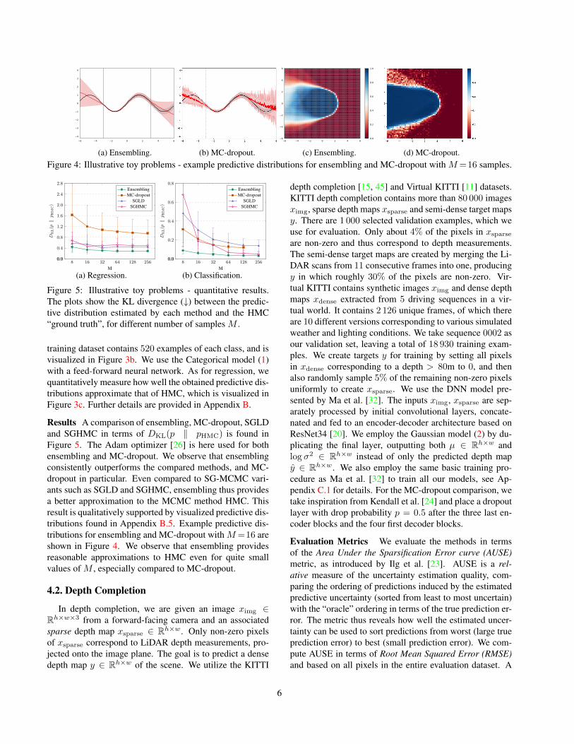
(c) Ensembling. (d) MC-dropout.Figure 4: Illustrative toy problems - example predictive distributions for ensembling and MC-dropout with M=16 samples.

8 16 32 64 128 2560.00.0

0.4

0.8

1.2

1.6

2.0

2.4

2.8

M

DKL(p‖pHM

C)

EnsemblingMC-dropout

SGLDSGHMC

(a) Regression.

8 16 32 64 128 2560.00.0

0.2

0.4

0.6

0.8

M

DKL(p‖pHM

C)

EnsemblingMC-dropout

SGLDSGHMC

(b) Classification.

Figure 5: Illustrative toy problems - quantitative results.The plots show the KL divergence (↓) between the predic-tive distribution estimated by each method and the HMC“ground truth”, for different number of samples M .

training dataset contains 520 examples of each class, and isvisualized in Figure 3b. We use the Categorical model (1)with a feed-forward neural network. As for regression, wequantitatively measure how well the obtained predictive dis-tributions approximate that of HMC, which is visualized inFigure 3c. Further details are provided in Appendix B.

Results A comparison of ensembling, MC-dropout, SGLDand SGHMC in terms of DKL(p ‖ pHMC) is found inFigure 5. The Adam optimizer [26] is here used for bothensembling and MC-dropout. We observe that ensemblingconsistently outperforms the compared methods, and MC-dropout in particular. Even compared to SG-MCMC vari-ants such as SGLD and SGHMC, ensembling thus providesa better approximation to the MCMC method HMC. Thisresult is qualitatively supported by visualized predictive dis-tributions found in Appendix B.5. Example predictive dis-tributions for ensembling and MC-dropout with M=16 areshown in Figure 4. We observe that ensembling providesreasonable approximations to HMC even for quite smallvalues of M , especially compared to MC-dropout.

4.2. Depth Completion

In depth completion, we are given an image ximg ∈Rh×w×3 from a forward-facing camera and an associatedsparse depth map xsparse ∈ Rh×w. Only non-zero pixelsof xsparse correspond to LiDAR depth measurements, pro-jected onto the image plane. The goal is to predict a densedepth map y ∈ Rh×w of the scene. We utilize the KITTI

depth completion [15, 45] and Virtual KITTI [11] datasets.KITTI depth completion contains more than 80 000 imagesximg, sparse depth maps xsparse and semi-dense target mapsy. There are 1 000 selected validation examples, which weuse for evaluation. Only about 4% of the pixels in xsparseare non-zero and thus correspond to depth measurements.The semi-dense target maps are created by merging the Li-DAR scans from 11 consecutive frames into one, producingy in which roughly 30% of the pixels are non-zero. Vir-tual KITTI contains synthetic images ximg and dense depthmaps xdense extracted from 5 driving sequences in a vir-tual world. It contains 2 126 unique frames, of which thereare 10 different versions corresponding to various simulatedweather and lighting conditions. We take sequence 0002 asour validation set, leaving a total of 18 930 training exam-ples. We create targets y for training by setting all pixelsin xdense corresponding to a depth > 80m to 0, and thenalso randomly sample 5% of the remaining non-zero pixelsuniformly to create xsparse. We use the DNN model pre-sented by Ma et al. [32]. The inputs ximg, xsparse are sep-arately processed by initial convolutional layers, concate-nated and fed to an encoder-decoder architecture based onResNet34 [20]. We employ the Gaussian model (2) by du-plicating the final layer, outputting both µ ∈ Rh×w andlog σ2 ∈ Rh×w instead of only the predicted depth mapy ∈ Rh×w. We also employ the same basic training pro-cedure as Ma et al. [32] to train all our models, see Ap-pendix C.1 for details. For the MC-dropout comparison, wetake inspiration from Kendall et al. [24] and place a dropoutlayer with drop probability p = 0.5 after the three last en-coder blocks and the four first decoder blocks.

Evaluation Metrics We evaluate the methods in termsof the Area Under the Sparsification Error curve (AUSE)metric, as introduced by Ilg et al. [23]. AUSE is a rel-ative measure of the uncertainty estimation quality, com-paring the ordering of predictions induced by the estimatedpredictive uncertainty (sorted from least to most uncertain)with the “oracle” ordering in terms of the true prediction er-ror. The metric thus reveals how well the estimated uncer-tainty can be used to sort predictions from worst (large trueprediction error) to best (small prediction error). We com-pute AUSE in terms of Root Mean Squared Error (RMSE)and based on all pixels in the entire evaluation dataset. A

6

1 2 4 8 16 320.04

0.06

0.08

0.10

M

AU

SEEnsemblingMC-dropout

(a) AUSE (↓).

1 2 4 8 16 320.000.00

0.04

0.08

0.12

0.16

0.20

0.24

M

AU

CE

EnsemblingMC-dropout

(b) AUCE (↓).

1 2 4 8 16 322,000

2,100

2,200

2,300

2,400

2,500

M

RM

SE[m

m]

EnsemblingMC-dropout

(c) RMSE (↓).

Figure 6: Depth completion - quantitative results. The plots show a comparison of ensembling and MC-dropout in terms ofAUSE, AUCE and RMSE on the KITTI depth completion validation dataset, for different number of samples M .

(a) Ensembling. (b) MC-dropout.

Figure 7: Depth completion - condensed calibration plotsfor ensembling and MC-dropout with M = 16.

perfect AUSE score can however be achieved even if thetrue predictive uncertainty is consistently underestimated.As an absolute measure of uncertainty estimation quality,we therefore also evaluate the methods in terms of cali-bration [5, 46]. In classification, the Expected CalibrationError (ECE) [17, 37] is a standard metric used to evalu-ate calibration. A well-calibrated model should then pro-duce classification confidences which match the observedprediction accuracy, meaning that the model is not over-confident (outputting highly confident predictions which areincorrect), nor over-conservative. We here employ a metricthat can be considered a natural generalization of ECE tothe regression setting. Since our models output the meanµ ∈ R and variance σ2 ∈ R of a Gaussian distribution foreach pixel, we can construct pixel-wise prediction intervalsµ ± Φ−1(p+1

2 )σ of confidence level p ∈]0, 1[, where Φ isthe CDF of the standard normal distribution. When comput-ing the proportion of pixels for which the prediction intervalcovers the true target y ∈ R, we expect this value, denotedp, to equal p ∈]0, 1[ for a perfectly calibrated model. Wecompute the absolute error with respect to perfect calibra-tion, |p − p|, for 100 values of p ∈]0, 1[ and use the areaunder this curve as our metric, which we call Area Underthe Calibration Error curve (AUCE). Lastly, we also evalu-ate in terms of the standard RMSE metric.

Results A comparison of ensembling and MC-dropout interms of AUSE, AUCE and RMSE on the KITTI depth com-pletion validation dataset is found in Figure 6. We observein Figure 6a that ensembling consistently outperforms MC-

dropout in terms of AUSE. However, the curves decrease asa function of M in a similar manner. Sparsification plotsand sparsification error curves are found in Appendix C.3.A ranking of the methods can be more readily conductedbased on Figure 6b, where we observe a clearly improvingtrend as M increases for ensembling, whereas MC-dropoutgets progressively worse. This result is qualitatively sup-ported by the calibration plots found in Appendix C.3 andFigure 7. Note that M = 1 corresponds to the baseline ofonly estimating aleatoric uncertainty.

4.3. Street-Scene Semantic Segmentation

In this task, we are given an image x ∈ Rh×w×3 froma forward-facing camera. The goal is to predict y of sizeh × w, in which each pixel is assigned to one of C dif-ferent class labels (road, sidewalk, car, etc.). We utilize thepopular Cityscapes [10] and recent Synscapes [49] datasets.Cityscapes contains 5 000 finely annotated images, mainlycollected in various German cities. The annotations in-cludes 30 class labels, but only C = 19 are used in thetraining of models. Its validation set contains 500 exam-ples, which we use for evaluation. Synscapes contains25 000 synthetic images, all captured in virtual urban envi-ronments. To match the size of Cityscapes, we randomlyselect 2 975 of these for training and 500 for validation.The images are annotated with the same class labels asCityscapes. We use the DeepLabv3 DNN model presentedby Chen et al. [6]. The input image x is processed by aResNet101 [20], outputting a feature map of stride 8. Thefeature map is further processed by an ASPP module anda 1 × 1 convolutional layer, outputting logits at 1/8 of theoriginal resolution. These are then upsampled to image res-olution using bilinear interpolation. The conventional Cat-egorical model (1) is thus used for each pixel. We base ourimplementation on the one by Yuan and Wang [51], and alsofollow the same basic training procedure, see Appendix D.1for details. For reference, the model obtains an mIoU [29]of 76.04% when trained on Cityscapes and evaluated on itsvalidation set. For the MC-dropout comparison, we take in-spiration from Mukhoti and Gal [36] and place a dropoutlayer with p = 0.5 after the four last ResNet blocks.

7

1 2 4 8 16

0.20

0.22

0.24

0.26

M

AU

SEEnsemblingMC-dropout

(a) AUSE (↓).

1 2 4 8 160.00

2.00

4.00

6.00

·10−2

M

EC

E

EnsemblingMC-dropout

(b) ECE (↓).

1 2 4 8 16

40

41

42

43

44

M

mIo

U[%

]

EnsemblingMC-dropout

(c) mIoU (↑).

Figure 8: Street-scene semantic segmentation - quantitative results. The plots show a comparison of ensembling and MC-dropout in terms of AUSE, ECE and mIoU on the Cityscapes validation dataset, for different number of samples M .

(a) Ensembling. (b) MC-dropout.

Figure 9: Street-scene semantic segmentation - example re-liability diagrams for the two methods with M = 16.

Evaluation Metrics As for depth completion, we evaluatethe methods in terms of the AUSE metric. In this classifi-cation setting, we compare the “oracle” ordering of predic-tions with the one induced by the predictive entropy. Wecompute AUSE in terms of Brier score and based on allpixels in the evaluation dataset. We also evaluate in termsof calibration by the ECE metric [17, 37]. All predictionsare here partitioned into L bins based on the maximum as-signed confidence. For each bin, the difference between theaverage predicted confidence and the actual accuracy is thencomputed, and ECE is obtained as the weighted average ofthese differences. We use L = 10 bins of equal size.

Results A comparison of ensembling and MC-dropoutin terms of AUSE, ECE and mIoU on the Cityscapes val-idation dataset is found in Figure 8. We observe that themetrics clearly improve as functions of M for both ensem-bling and MC-dropout, demonstrating the importance ofepistemic uncertainty estimation. The rate of improvementis generally greater for ensembling. For ECE, we observein Figure 8b a drastic improvement for ensembling as M isincreased, followed by a distinct plateau. According to thecondensed reliability diagrams in Appendix D.3, this cor-responds to a transition from clear model over-confidenceto slight over-conservatism. For MC-dropout, the corre-sponding diagrams suggest a stagnation while the modelstill is somewhat over-confident. Example reliability dia-grams for M = 16 are shown in Figure 9, in which thisover-confidence for MC-dropout can be observed. Note

that the relatively low mIoU scores reported in Figure 8c,obtained by models trained exclusively on Synscapes, areexpected [49] and caused by the intentionally challengingdomain gap between synthetic and real-world data.

5. Discussion & ConclusionWe proposed a comprehensive evaluation framework for

scalable epistemic uncertainty estimation methods in deeplearning. The proposed framework is specifically designedto test the robustness required in real-world computer visionapplications. We applied our proposed framework and pro-vided the first properly extensive and conclusive compar-ison of ensembling and MC-dropout, the results of whichdemonstrates that ensembling consistently provides morereliable and practically useful uncertainty estimates. Weattribute the success of ensembling to its ability, due tothe random initialization, to capture the important aspect ofmulti-modality present in the posterior distribution p(θ|D)of DNNs. MC-dropout has a large design-space comparedto ensembling, and while careful tuning of MC-dropoutpotentially could close the performance gap on individualtasks, the simplicity and general applicability of ensem-bling must be considered key strengths. The main draw-back of both methods is the computational cost at test timethat grows linearly with M , limiting real-time applicability.Here, future work includes exploring the effect of modelpruning techniques [50, 18] on predictive uncertainty qual-ity. For ensembling, sharing early stages of the DNN amongensemble members is also an interesting future direction. Aweakness of ensembling is the additional training required,which also scales linearly with M . The training of differentensemble members can however be performed in parallel,making it less of an issue in practice given appropriate com-puting infrastructure. In conclusion, our work suggests thatensembling should be considered the new go-to method forscalable epistemic uncertainty estimation.

Acknowledgments This research was supported by theSwedish Foundation for Strategic Research via the projectASSEMBLE and by the Swedish Research Council via theproject Learning flexible models for nonlinear dynamics.

8

References[1] Peter Auer, Mark Herbster, and Manfred K Warmuth. Expo-

nentially many local minima for single neurons. In Advancesin Neural Information Processing Systems (NeurIPS), pages316–322, 1996. 5

[2] David Barber and Christopher M Bishop. Ensemble learningin Bayesian neural networks. Nato ASI Series F Computerand Systems Sciences, 168:215–238, 1998. 5

[3] Eli Bingham, Jonathan P. Chen, Martin Jankowiak, FritzObermeyer, Neeraj Pradhan, Theofanis Karaletsos, RohitSingh, Paul Szerlip, Paul Horsfall, and Noah D. Goodman.Pyro: Deep Universal Probabilistic Programming. Journalof Machine Learning Research, 2018. 11

[4] Charles Blundell, Julien Cornebise, Koray Kavukcuoglu,and Daan Wierstra. Weight uncertainty in neural network.In International Conference on Machine Learning (ICML),pages 1613–1622, 2015. 2, 5

[5] Jochen Brocker. Reliability, sufficiency, and the decomposi-tion of proper scores. Quarterly Journal of the Royal Mete-orological Society, 135(643):1512–1519, 2009. 7

[6] Liang-Chieh Chen, George Papandreou, Florian Schroff, andHartwig Adam. Rethinking atrous convolution for seman-tic image segmentation. arXiv preprint arXiv:1706.05587,2017. 1, 7

[7] Tianqi Chen, Emily Fox, and Carlos Guestrin. Stochasticgradient Hamiltonian Monte Carlo. In International Confer-ence on Machine Learning (ICML), pages 1683–1691, 2014.2, 4

[8] Anna Choromanska, Mikael Henaff, Michael Mathieu,Gerard Ben Arous, and Yann LeCun. The loss surfaces ofmultilayer networks. In Artificial Intelligence and Statistics,pages 192–204, 2015. 5

[9] Kurtland Chua, Roberto Calandra, Rowan McAllister, andSergey Levine. Deep reinforcement learning in a handfulof trials using probabilistic dynamics models. In Advancesin Neural Information Processing Systems (NeurIPS), pages4759–4770, 2018. 1, 2, 3

[10] Marius Cordts, Mohamed Omran, Sebastian Ramos, TimoRehfeld, Markus Enzweiler, Rodrigo Benenson, UweFranke, Stefan Roth, and Bernt Schiele. The cityscapesdataset for semantic urban scene understanding. In Proceed-ings of the IEEE Conference on Computer Vision and PatternRecognition (CVPR), pages 3213–3223, 2016. 1, 2, 7

[11] A Gaidon, Q Wang, Y Cabon, and E Vig. Virtual worldsas proxy for multi-object tracking analysis. In Proceedingsof the IEEE Conference on Computer Vision and PatternRecognition (CVPR), 2016. 2, 6

[12] Yarin Gal. Uncertainty in Deep Learning. PhD thesis, Uni-versity of Cambridge, 2016. 1, 2

[13] Yarin Gal and Zoubin Ghahramani. Dropout as a Bayesianapproximation: Representing model uncertainty in deeplearning. In International Conference on Machine Learning(ICML), pages 1050–1059, 2016. 5

[14] Jochen Gast and Stefan Roth. Lightweight probabilistic deepnetworks. In Proceedings of the IEEE Conference on Com-puter Vision and Pattern Recognition (CVPR), pages 3369–3378, 2018. 1

[15] Andreas Geiger, Philip Lenz, Christoph Stiller, and RaquelUrtasun. Vision meets robotics: The KITTI dataset. Interna-tional Journal of Robotics Research (IJRR), 2013. 2, 6

[16] Alex Graves. Practical variational inference for neural net-works. In Advances in Neural Information Processing Sys-tems (NeurIPS), pages 2348–2356, 2011. 5

[17] Chuan Guo, Geoff Pleiss, Yu Sun, and Kilian Q Weinberger.On calibration of modern neural networks. In Proceedingsof the 34th International Conference on Machine Learning(ICML), pages 1321–1330, 2017. 1, 7, 8

[18] Song Han, Huizi Mao, and William J Dally. Deep com-pression: Compressing deep neural networks with pruning,trained quantization and Huffman coding. In InternationalConference on Learning Representations (ICLR), 2016. 8

[19] W Keith Hastings. Monte Carlo sampling methods usingMarkov chains and their applications. Biometrika, 57(1):97–109, 1970. 4

[20] Kaiming He, Xiangyu Zhang, Shaoqing Ren, and Jian Sun.Deep residual learning for image recognition. In Proceed-ings of the IEEE Conference on Computer Vision and PatternRecognition (CVPR), pages 770–778, 2016. 6, 7

[21] Jose Miguel Hernandez-Lobato and Ryan Adams. Prob-abilistic backpropagation for scalable learning of bayesianneural networks. In International Conference on MachineLearning (ICML), pages 1861–1869, 2015. 2

[22] Geoffrey Hinton and Drew Van Camp. Keeping neural net-works simple by minimizing the description length of theweights. In Proceedings of the 6th Annual ACM Conferenceon Computational Learning Theory (COLT), 1993. 2, 5

[23] Eddy Ilg, Ozgun Cicek, Silvio Galesso, Aaron Klein, OsamaMakansi, Frank Hutter, and Thomas Bro. Uncertainty es-timates and multi-hypotheses networks for optical flow. InProceedings of the European Conference on Computer Vi-sion (ECCV), pages 652–667, 2018. 1, 2, 3, 6

[24] Alex Kendall, Vijay Badrinarayanan, and Roberto Cipolla.Bayesian SegNet: Model uncertainty in deep convolu-tional encoder-decoder architectures for scene understand-ing. In Proceedings of the British Machine Vision Confer-ence (BMVC), 2017. 2, 5, 6

[25] Alex Kendall and Yarin Gal. What uncertainties do we needin Bayesian deep learning for computer vision? In Advancesin Neural Information Processing Systems (NeurIPS), pages5574–5584, 2017. 1, 2, 3

[26] Diederik P Kingma and Jimmy Ba. Adam: A method forstochastic optimization. arXiv preprint arXiv:1412.6980,2014. 6

[27] Balaji Lakshminarayanan, Alexander Pritzel, and CharlesBlundell. Simple and scalable predictive uncertainty estima-tion using deep ensembles. In Advances in Neural Informa-tion Processing Systems (NeurIPS), pages 6402–6413, 2017.1, 2, 3, 5

[28] Alex H Lang, Sourabh Vora, Holger Caesar, Lubing Zhou,Jiong Yang, and Oscar Beijbom. PointPillars: Fast encodersfor object detection from point clouds. In Proceedings of theIEEE Conference on Computer Vision and Pattern Recogni-tion (CVPR), 2019. 1, 3

9

[29] Jonathan Long, Evan Shelhamer, and Trevor Darrell. Fullyconvolutional networks for semantic segmentation. In Pro-ceedings of the IEEE Conference on Computer Vision andPattern Recognition (CVPR), pages 3431–3440, 2015. 8

[30] Christos Louizos and Max Welling. Structured and efficientvariational deep learning with matrix Gaussian posteriors. InProceedings of the 33rd International Conference on Ma-chine Learning (ICML), pages 1708–1716, 2016. 5

[31] Christos Louizos and Max Welling. Multiplicative normal-izing flows for variational Bayesian neural networks. In Pro-ceedings of the 34th International Conference on MachineLearning (ICML), pages 2218–2227, 2017. 5

[32] Fangchang Ma, Guilherme Venturelli Cavalheiro, and SertacKaraman. Self-supervised sparse-to-dense: Self-superviseddepth completion from LiDAR and monocular camera.In Proceedings of the IEEE International Conference onRobotics and Automation (ICRA), 2019. 1, 6, 16

[33] Yi-An Ma, Tianqi Chen, and Emily Fox. A complete recipefor stochastic gradient MCMC. In Advances in Neural In-formation Processing Systems (NeurIPS), pages 2917–2925,2015. 4

[34] Andrey Malinin and Mark Gales. Predictive uncertainty es-timation via prior networks. In Advances in Neural Informa-tion Processing Systems (NeurIPS), pages 7047–7058, 2018.1

[35] Nicholas Metropolis, Arianna W Rosenbluth, Marshall NRosenbluth, Augusta H Teller, and Edward Teller. Equa-tion of state calculations by fast computing machines. Thejournal of chemical physics, 21(6):1087–1092, 1953. 4

[36] Jishnu Mukhoti and Yarin Gal. Evaluating Bayesian deeplearning methods for semantic segmentation. arXiv preprintarXiv:1811.12709, 2018. 2, 5, 8

[37] Mahdi Pakdaman Naeini, Gregory Cooper, and MilosHauskrecht. Obtaining well calibrated probabilities usingBayesian binning. In Twenty-Ninth AAAI Conference on Ar-tificial Intelligence, 2015. 7, 8

[38] Radford M Neal. Bayesian learning for neural networks.PhD thesis, University of Toronto, 1995. 2, 4

[39] Radford M Neal. MCMC using Hamiltonian dynamics.Handbook of Markov chain Monte Carlo, 2:113–162, 2011.4, 5

[40] Adam Paszke, Sam Gross, Soumith Chintala, GregoryChanan, Edward Yang, Zachary DeVito, Zeming Lin, Al-ban Desmaison, Luca Antiga, and Adam Lerer. Automaticdifferentiation in PyTorch. In NeurIPS - Autodiff Workshop,2017. 5

[41] Murat Sensoy, Lance Kaplan, and Melih Kandemir. Evi-dential deep learning to quantify classification uncertainty.In Advances in Neural Information Processing Systems(NeurIPS), pages 3179–3189, 2018. 1

[42] Shaoshuai Shi, Xiaogang Wang, and Hongsheng Li. PointR-CNN: 3D object proposal generation and detection frompoint cloud. In Proceedings of the IEEE Conference on Com-puter Vision and Pattern Recognition (CVPR), 2019. 1, 3

[43] Jasper Snoek, Yaniv Ovadia, Emily Fertig, Balaji Lakshmi-narayanan, Sebastian Nowozin, D Sculley, Joshua Dillon, JieRen, and Zachary Nado. Can you trust your model’s un-certainty? Evaluating predictive uncertainty under dataset

shift. In Advances in Neural Information Processing Systems(NeurIPS), pages 13969–13980, 2019. 2

[44] Nitish Srivastava, Geoffrey Hinton, Alex Krizhevsky, IlyaSutskever, and Ruslan Salakhutdinov. Dropout: a simple wayto prevent neural networks from overfitting. The Journal ofMachine Learning Research, 15(1):1929–1958, 2014. 5

[45] Jonas Uhrig, Nick Schneider, Lukas Schneider, Uwe Franke,Thomas Brox, and Andreas Geiger. Sparsity invariant CNNs.In International Conference on 3D Vision (3DV), 2017. 1, 2,6

[46] Juozas Vaicenavicius, David Widmann, Carl Andersson,Fredrik Lindsten, Jacob Roll, and Thomas B Schon. Eval-uating model calibration in classification. In Proceedings ofthe International Conference on Artificial Intelligence andStatistics (AISTATS), 2019. 7

[47] Hao Wang, SHI Xingjian, and Dit-Yan Yeung. Natural-parameter networks: A class of probabilistic neural net-works. In Advances in Neural Information Processing Sys-tems (NeurIPS), pages 118–126, 2016. 2

[48] Max Welling and Yee W Teh. Bayesian learning via stochas-tic gradient Langevin dynamics. In International Conferenceon Machine Learning (ICML), pages 681–688, 2011. 2, 4

[49] Magnus Wrenninge and Jonas Unger. Synscapes: A pho-torealistic synthetic dataset for street scene parsing. arXivpreprint arXiv:1810.08705, 2018. 2, 7, 8

[50] Tien-Ju Yang, Yu-Hsin Chen, and Vivienne Sze. Designingenergy-efficient convolutional neural networks using energy-aware pruning. In Proceedings of the IEEE Conference onComputer Vision and Pattern Recognition (CVPR), pages5687–5695, 2017. 8

[51] Yuhui Yuan and Jingdong Wang. Ocnet: Object context net-work for scene parsing. arXiv preprint arXiv:1809.00916,2018. 1, 8, 23

[52] Guodong Zhang, Shengyang Sun, David Duvenaud, andRoger Grosse. Noisy natural gradient as variational infer-ence. In Proceedings of the 35th International Conferenceon Machine Learning (ICML), pages 5847–5856, 2018. 5

[53] Ruqi Zhang, Chunyuan Li, Jianyi Zhang, Changyou Chen,and Andrew Gordon Wilson. Cyclical stochastic gradi-ent MCMC for Bayesian deep learning. arXiv preprintarXiv:1902.03932, 2019. 5

10

Supplementary MaterialThis is the supplementary material for Evaluating Scalable Bayesian Deep Learning Methods for Robust Computer

Vision. It consists of Appendix A-D.

Appendix A. Approximating a Mixture of Gaussian DistributionsFor the Gaussian model (2), p(y?|x?,D) in (4) is a uniformly weighted mixture of Gaussian distributions. We approximate

this mixture with a single Gaussian parameterized by the mixture mean and variance:

p(y?|x?,D) =1

M

M∑i=1

p(y?|x?, θ(i)), θ(i) ∼ q(θ),

p(y?|x?,D) =1

M

M∑i=1

N (y?;µθ(i)(x?), σ2

θ(i)(x?)), θ(i) ∼ q(θ),

p(y?|x?,D) ≈ N (y?; µ(x?), σ2(x?)),

µ(x) =1

M

M∑i=1

µθ(i)(x), σ2(x) =1

M

M∑i=1

((µθ(i)(x)− µ(x)

)2+ σ2

θ(i)(x)

), θ(i) ∼ q(θ).

Appendix B. Illustrative Toy ProblemsIn this appendix, further details on the illustrative toy problems experiments (Section 4.1) are provided.

B.1. Experimental Setup

Figure 5a (regression) shows DKL(p ‖ pHMC) computed on [−7, 7]. All training data was given in [−3, 3].Figure 5b (classification) shows DKL(p ‖ pHMC) computed on the region−6 ≤ x1 ≤ 6, −6 ≤ x2 ≤ 6. All training data

was given in the region 0 ≤ x1 ≤ 3, −3 ≤ x2 ≤ 3.For regression, DKL(p ‖ pHMC) is computed using the formula for KL divergence between two Gaussian distributions

p1(x) = N (x;µ1, σ21), p2(x) = N (x;µ2, σ

22):

DKL(p1 ‖ p2) = logσ2σ1

+σ21 + (µ1 − µ2)2

2σ22

− 1

2.

For classification, DKL(p ‖ pHMC) is computed using the formula for KL divergence between two discrete distributionsq1(x), q2(x):

DKL(q1 ‖ q2) =∑x∈X

q1(x) logq1(x)

q2(x).

For both regression and classification, HMC with prior p(θ) = N (0, IP ) and M = 1 000 samples is implemented usingPyro [3]. Specifically, we use pyro.infer.mcmc.MCMC with pyro.infer.mcmc.NUTS as kernel, num samples = 1 000 andwarmup steps = 1 000.

B.2. Implementation Details

For regression, we use the Gaussian model (2) with two separate feed-forward neural networks outputting µθ(x) andlog σ2

θ(x). Both neural networks have 2 hidden layers of size 10.For classification, we use the Categorical model (1) with a feed-forward neural network with 2 hidden layers of size 10.For the MC-dropout comparison, we place a dropout layer after the first hidden layer of each neural network. For regres-

sion, we use a drop probability p = 0.2. For classification, we use p = 0.1.For ensembling, we train all ensemble models for 150 epochs with the Adam optimizer, a batch size of 32 and a fixed

learning rate of 0.001.For MC-dropout, we train models for 300 epochs with the Adam optimizer, a batch size of 32 and a fixed learning rate of

0.001.

11

For ensembling and MC-dropout, we minimize the MAP objective − log p(Y |X, θ)p(θ). In our case where the modelparameters θ ∈ RP and p(θ) = N (0, IP ), this corresponds to the following loss for regression:

L(θ) =1

N

N∑i=1

(yi − µ(xi))2

σ2(xi)+ log σ2(xi) +

1

NθTθ.

For classification, where yi = [ yi,1 . . . yi,C ]T (one-hot encoded) and s(xi) = [ s(xi)1 . . . s(xi)C ]

T is the Softmax output, itcorresponds to the following loss:

L(θ) = − 1

N

N∑i=1

C∑k=1

yi,k log s(xi)k +1

2NθTθ.

For SGLD, we extract samples from the parameter trajectory given by the update equation:

θt+1 = θt − αt∇θU(θt) +√

2αtεt,

where εt ∼ N (0, 1), ∇θU(θ) is the stochastic gradient of U(θ) = − log p(Y |X, θ)p(θ) and αt is the stepsize. We run it fora total number of steps corresponding to 256 · 150 epochs with a batch size of 32. The stepsize αt is decayed according to:

αt = α0(1− t

T)0.9, t = 1, 2, . . . , T,

where T is the total number of steps, α0 = 0.01 (the initial stepsize) for regression and α0 = 0.05 for classification.M ∈ {8, 16, 32, 64, 128, 256} samples are extracted starting at step t = int(0.75T ), ending at step t = T and spread outevenly between.

For SGHMC, we extract samples from the parameter trajectory given by the update equation:

θt+1 = θt + rt,

rt+1 = (1− η)rt − αt∇θU(θt) +√

2ηαtεt,

where εt ∼ N (0, 1), ∇θU(θ) is the stochastic gradient of U(θ) = − log p(Y |X, θ)p(θ), αt is the stepsize and η = 0.1.We run it for a total number of steps corresponding to 256 · 150 epochs with a batch size of 32. The stepsize αt is decayedaccording to:

αt = α0(1− t

T)0.9, t = 1, 2, . . . , T,

where T is the total number of steps, α0 = 0.001 (the initial stepsize) for regression and α0 = 0.01 for classification.M ∈ {8, 16, 32, 64, 128, 256} samples are extracted starting at step t = int(0.75T ), ending at step t = T and spread outevenly between.

For all models, we randomly initialize the parameters θ using the default initializer in PyTorch.

B.3. Description of Results

The results in Figure 5a, 5b were obtained in the following way:

• Ensembling: 1024 models were trained using the same training procedure, the mean and standard deviation was com-puted based on 1024/M unique sets of models for M ∈ {8, 16, 32, 64, 128, 256}.

• MC-dropout: 10 models were trained using the same training procedure, based on which the mean and standarddeviation was computed.

• SGLD: 6 models were trained using the same training procedure, based on which the mean and standard deviation wascomputed.

• SGHMC: 6 models were trained using the same training procedure, based on which the mean and standard deviationwas computed.

12

101 1020.0

1.0

2.0

3.0

4.0

M

DKL(p‖pHM

C)

Ensembling - SGDMC-dropout - SGD

SGLDSGHMC

(a) Regression

101 1020.0

0.2

0.4

0.6

0.8

1.0

M

DKL(p‖pHM

C)

Ensembling - SGDMC-dropout - SGD

SGLDSGHMC

(b) Classification

Figure 10: Illustrative toy problems, quantitative results. SGD is used for ensembling and MC-dropout instead of Adam.

101 1020.0

1.0

2.0

3.0

4.0

M

DKL(p‖pHM

C)

Ensembling - SGDMOMMC-dropout - SGDMOM

SGLDSGHMC

(a) Regression

101 1020.0

0.2

0.4

0.6

0.8

1.0

M

DKL(p‖pHM

C)

Ensembling - SGDMOMMC-dropout - SGDMOM

SGLDSGHMC

(b) Classification

Figure 11: Illustrative toy problems, quantitative results. SGD with momentum is used for ensembling and MC-dropoutinstead of Adam.

101 1020.0

2.0

4.0

6.0

8.0

10.0

M

DKL(p‖pHM

C)

Ensembling - SGDMOMMC-dropout - SGDMOM

SGLD-64SGHMC-64

Figure 12: Illustrative toy regression problem, quantitative results. SGD with momentum is used for ensembling and MC-dropout instead of Adam. Less training for SGLD and SGHMC.

B.4. Additional Results

Figure 10 and Figure 11 show the same comparison as Figure 5a, 5b, but using SGD and SGD with momentum forensembling and MC-dropout, respectively. We observe that ensembling consistently outperforms the compared methodsfor classification, but that SGLD and SGHMC has better performance for regression in these cases. SGLD and SGHMCare however trained for 256 times longer than each ensemble model, complicating the comparison somewhat. If SGLDand SGHMC instead are trained for just 64 times longer than each ensemble model, we observe in Figure 12 that they areconsistently outperformed by ensembling.

For MC-dropout using Adam, we also varied the drop probability p and chose the best performing variant. These resultsare found in Figure 13, in which * marks the chosen variant.

B.5. Qualitative Results

Here, we show visualizations of predictive distributions obtained by the different methods. Figure 14, 18 for ensembling,Figure 15, 19 for MC-dropout, Figure 16, 20 for SGLD, and Figure 17, 21 for SGHMC.

13

101 1020.0

2.0

4.0

6.0

8.0

M

DKL(p‖pHM

C)

p = 0.05p = 0.1

*p = 0.2

(a) Regression

101 1020.0

0.2

0.4

0.6

0.8

1.0

1.2

M

DKL(p‖pHM

C)

p = 0.05*p = 0.1p = 0.2p = 0.5

(b) Classification

Figure 13: Illustrative toy problems, quantitative results. MC-dropout using Adam.

Figure 14: Toy regression problem, ensembling, M = 64. Examples of predictive distributions.

Figure 15: Toy regression problem, MC-dropout, M = 64. Examples of predictive distributions.

Figure 16: Toy regression problem, SGLD, M = 64. Examples of predictive distributions.

Figure 17: Toy regression problem, SGHMC, M = 64. Examples of predictive distributions.

14

Figure 18: Toy classification problem, ensembling, M = 64. Examples of predictive distributions.

Figure 19: Toy classification problem, MC-dropout, M = 64. Examples of predictive distributions.

Figure 20: Toy classification problem, SGLD, M = 64. Examples of predictive distributions.

Figure 21: Toy classification problem, SGHMC, M = 64. Examples of predictive distributions.

15

Appendix C. Depth CompletionIn this appendix, further details on the depth completion experiments (Section 4.2) are provided.

C.1. Training Details

For both ensembling and MC-dropout, we train all models for 40 000 steps with the Adam optimizer, a batch size of 4,a fixed learning rate of 10−5 and weight decay of 0.0005. We use a smaller batch size and train for fewer steps than Ma etal. [32] to enable an extensive evaluation with repeated experiments. For the same reason, we also train on randomly selectedimage crops of size 352× 352. The only other data augmentation used is random flipping along the vertical axis. We followMa et al. [32] and randomly initialize all network weights from N (0, 10−3) and all network biases with 0s. Models aretrained on a single NVIDIA TITAN Xp GPU with 12GB of RAM.

C.2. Description of Results

The results in Figure 6 (Section 4.2) were obtained in the following way:

• Ensembling: 33 models were trained using the same training procedure, the mean and standard deviation was computedbased on 32 (M = 1), 16 (M = 2, 4, 8, 16) or 4 (M = 32) sets of randomly drawn models. The same set could not bedrawn more than once.

• MC-dropout: 16 models were trained using the same training procedure, based on which the mean and standarddeviation was computed.

C.3. Additional Results

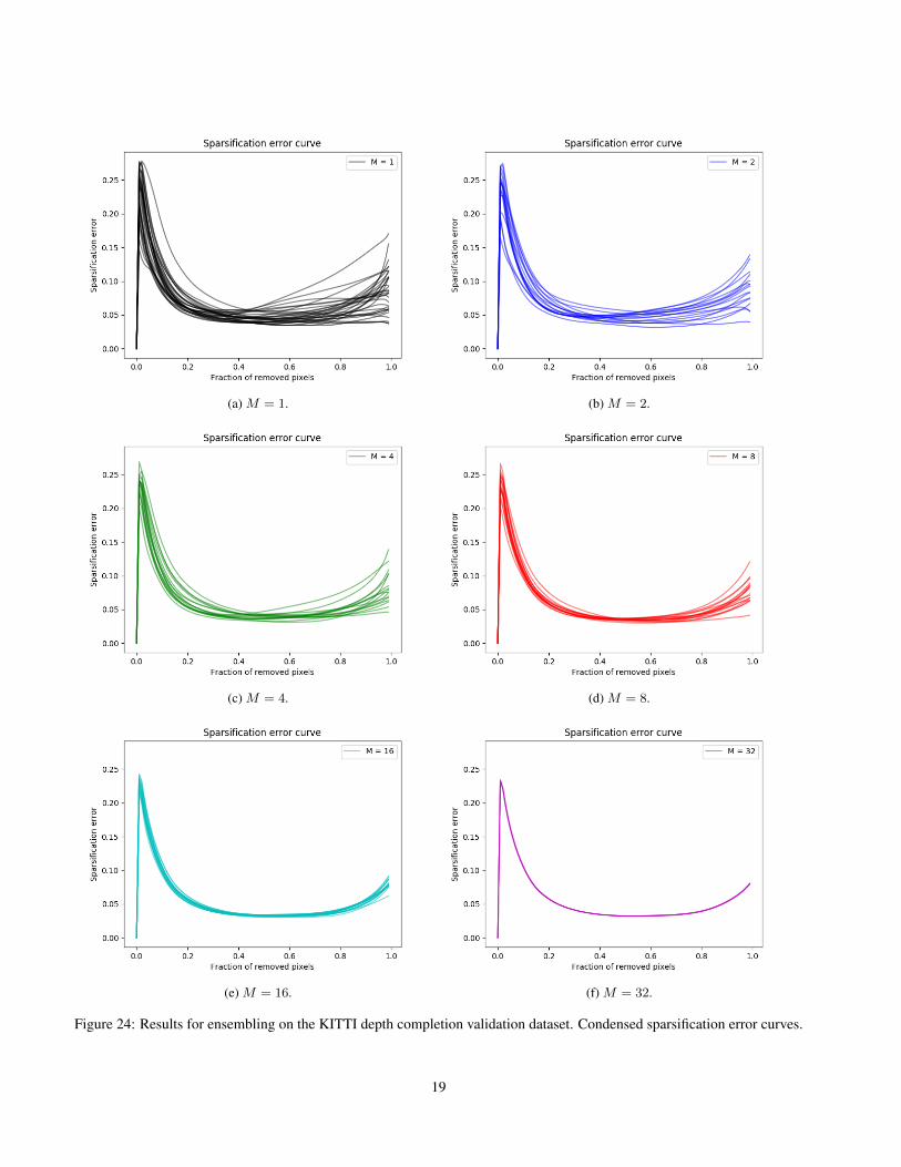
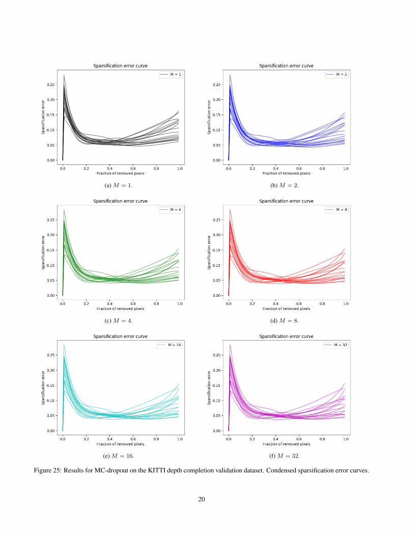
Here, we show sparsification plots, sparsification error curves and calibration plots. Examples of sparsification plotsare found in Figure 22 for ensembling and Figure 23 for MC-dropout. Condensed sparsification error curves are found inFigure 24 for ensembling and Figure 25 for MC-dropout. Condensed calibration plots are found in Figure 26 for ensemblingand Figure 27 for MC-dropout.

16

(a) M = 1. (b) M = 2.

(c) M = 4. (d) M = 8.

(e) M = 16. (f) M = 32.

Figure 22: Results for ensembling on the KITTI depth completion validation dataset. Examples of sparsification plots.

17

(a) M = 1. (b) M = 2.

(c) M = 4. (d) M = 8.

(e) M = 16. (f) M = 32.

Figure 23: Results for MC-dropout on the KITTI depth completion validation dataset. Examples of sparsification plots.

18

(a) M = 1. (b) M = 2.

(c) M = 4. (d) M = 8.

(e) M = 16. (f) M = 32.

Figure 24: Results for ensembling on the KITTI depth completion validation dataset. Condensed sparsification error curves.

19

(a) M = 1. (b) M = 2.

(c) M = 4. (d) M = 8.

(e) M = 16. (f) M = 32.

Figure 25: Results for MC-dropout on the KITTI depth completion validation dataset. Condensed sparsification error curves.

20

(a) M = 1. (b) M = 2.

(c) M = 4. (d) M = 8.

(e) M = 16. (f) M = 32.

Figure 26: Results for ensembling on the KITTI depth completion validation dataset. Condensed calibration plots.

21

(a) M = 1. (b) M = 2.

(c) M = 4. (d) M = 8.

(e) M = 16.

Figure 27: Results for MC-dropout on the KITTI depth completion validation dataset. Condensed calibration plots.

22

Appendix D. Street-Scene Semantic SegmentationIn this appendix, further details on the street-scene semantic segmentation experiments (Section 4.3) are provided.

D.1. Training Details

For ensembling, we train all ensemble models for 40 000 steps with SGD + momentum (0.9), a batch size of 8 and weightdecay of 0.0005. The learning rate αt is decayed according to:

αt = α0(1− t

T)0.9, t = 1, 2, . . . , T,

where T = 40 000 and α0 = 0.01 (the initial learning rate). We train on randomly selected image crops of size 512 × 512.We choose a smaller crop size than Yuan and Wang [51] to enable an extensive evaluation with repeated experiments. Theonly other data augmentation used is random flipping along the vertical axis and random scaling in the range [0.5, 1.5]. TheResNet101 backbone is initialized with weights1 from a model pretrained on the ImageNet dataset, all other model parametersare randomly initialized using the default initializer in PyTorch. Models are trained on two NVIDIA TITAN Xp GPUs with12GB of RAM each. For MC-dropout, models are instead trained for 60 000 steps.

D.2. Description of Results

The results in Figure 8 (Section 4.3) were obtained in the following way:

• Ensembling: 26 models were trained using the same training procedure, the mean and standard deviation was computedbased on 8 sets of randomly drawn models for M ∈ {1, 2, 4, 8, 16}. The same set could not be drawn more than once.

• MC-dropout: 8 models were trained using the same training procedure, based on which the mean and standard deviationwas computed.

D.3. Additional Results

Here, we show sparsification plots, sparsification error curves and reliability diagrams. Examples of sparsification plotsare found in Figure 28 for ensembling and Figure 29 for MC-dropout. Condensed sparsification error curves are foundin Figure 30 for ensembling and Figure 31 for MC-dropout. Examples of reliability diagrams with histograms are foundin Figure 32 for ensembling and Figure 33 for MC-dropout. Condensed reliability diagrams are found in Figure 34 forensembling and Figure 35 for MC-dropout.

1http://sceneparsing.csail.mit.edu/model/pretrained_resnet/resnet101-imagenet.pth.

23

(a) M = 1. (b) M = 2.

(c) M = 4. (d) M = 8.

(e) M = 16.

Figure 28: Results for ensembling on the Cityscapes validation dataset. Examples of sparsification plots.

24

(a) M = 1. (b) M = 2.

(c) M = 4. (d) M = 8.

(e) M = 16.

Figure 29: Results for MC-dropout on the Cityscapes validation dataset. Examples of sparsification plots.

25

(a) M = 1. (b) M = 2.

(c) M = 4. (d) M = 8.

(e) M = 16.

Figure 30: Results for ensembling on the Cityscapes validation dataset. Condensed sparsification error curves.

26

(a) M = 1. (b) M = 2.

(c) M = 4. (d) M = 8.

(e) M = 16.

Figure 31: Results for MC-dropout on the Cityscapes validation dataset. Condensed sparsification error curves.

27

(a) M = 1. (b) M = 2.

(c) M = 4. (d) M = 8.

(e) M = 16.

Figure 32: Results for ensembling on the Cityscapes validation dataset. Examples of reliability diagrams with histograms.

28

(a) M = 1. (b) M = 2.

(c) M = 4. (d) M = 8.

(e) M = 16.

Figure 33: Results for MC-dropout on the Cityscapes validation dataset. Examples of reliability diagrams with histograms.

29

(a) M = 1. (b) M = 2.

(c) M = 4. (d) M = 8.

(e) M = 16.

Figure 34: Results for ensembling on the Cityscapes validation dataset. Condensed reliability diagrams.

30

(a) M = 1. (b) M = 2.

(c) M = 4. (d) M = 8.

(e) M = 16.

Figure 35: Results for MC-dropout on the Cityscapes validation dataset. Condensed reliability diagrams.

31