beyond gdp? welfare across countries and timeklenow.com/jones_klenow_slides.pdfbeyond gdp? welfare...

Beyond GDP?Welfare across Countries and Time

Chad Jones and Pete Klenow

Stanford University and NBER

November 10, 2010

Comparing welfare across countries and over time

How successful is an economy at delivering the highest possiblewelfare for its citizens?

• Fundamental question at the heart of economic growth anddevelopment

• Per capita GDP is our standard (shortcut) answer

• Can we do better?

GDP per capita 6= Welfare

Utility depends on:

• Consumption

• Life Expectancy

• Leisure

• Inequality

• ...

But GDP per capita “only” measures income...

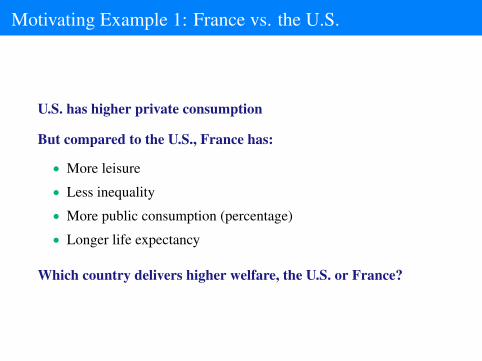
Motivating Example 1: France vs. the U.S.

U.S. has higher private consumption

But compared to the U.S., France has:

• More leisure

• Less inequality

• More public consumption (percentage)

• Longer life expectancy

Which country delivers higher welfare, the U.S. or France?

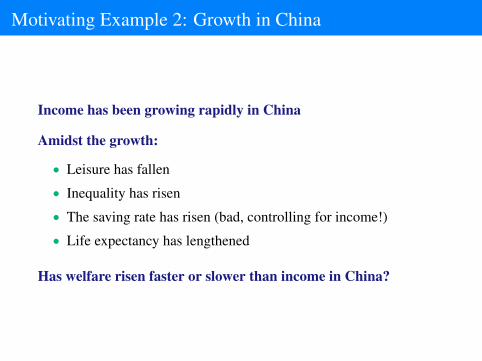
Motivating Example 2: Growth in China

Income has been growing rapidly in China

Amidst the growth:

• Leisure has fallen

• Inequality has risen

• The saving rate has risen (bad, controlling for income!)

• Life expectancy has lengthened

Has welfare risen faster or slower than income in China?

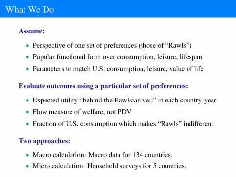
What We Do

Assume:

• Perspective of one set of preferences (those of “Rawls”)

• Popular functional form over consumption, leisure, lifespan

• Parameters to match U.S. consumption, leisure, value of life

Evaluate outcomes using a particular set of preferences:

• Expected utility “behind the Rawlsian veil” in each country-year

• Flow measure of welfare, not PDV

• Fraction of U.S. consumption which makes “Rawls” indifferent

Two approaches:

• Macro calculation: Macro data for 134 countries.• Micro calculation: Household surveys for 5 countries.

Important Shortcomings of our Approach

Factors we do not capture

• Morbidity (other than through health spending)

• Quality of the natural environment

• Political freedoms

• Crime

• ....

But neither does income!

Summary of Results

• Income and welfare are highly correlated in both levels andgrowth rates.

• Nevertheless, differences between income and welfare areeconomically important:

– Median deviation in levels is over 40 percent.

– Median deviation in growth rates is about 1 percentage point.

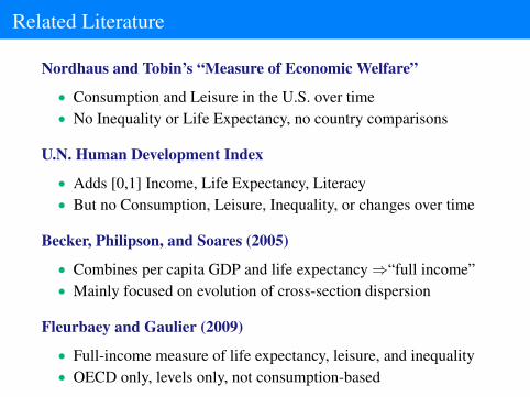
Related Literature

Nordhaus and Tobin’s “Measure of Economic Welfare”

• Consumption and Leisure in the U.S. over time• No Inequality or Life Expectancy, no country comparisons

U.N. Human Development Index

• Adds [0,1] Income, Life Expectancy, Literacy• But no Consumption, Leisure, Inequality, or changes over time

Becker, Philipson, and Soares (2005)

• Combines per capita GDP and life expectancy⇒“full income”• Mainly focused on evolution of cross-section dispersion

Fleurbaey and Gaulier (2009)

• Full-income measure of life expectancy, leisure, and inequality• OECD only, levels only, not consumption-based

Theory Underlyingthe Macro Calculations

Let Rawls “live” for a year as a random person in some country,facing their mortality rates and consumption/leisure distribution.

Overview of Welfare

Expected utility behind the Rawlsian veil of ignorance:

V(e, c, `, σ) = e(

u + log c + v(`)− 12σ2)

Preferences

• Let C denote an individual’s consumption.— Independent of age.

• Let ` denote leisure or time spent in home production.

• Flow utility in benchmark case

u(C, `) = u + log C + v(`)

• u influences the value of life given C, `.

Life Expectancy

• Rawls draws ageUniform[0,100]

• Faces thecross-sectionalmortality rates for2000 in a country

• p = probabilitylives instead of dies

p = e/100 0 1000

1

Age, a

Probability of Survival to Age a

LifeExpectancy, e

• Expected utility — normalizing death to be 0:

p · u(C, `) + (1− p) · 0 = e · u(C, `)/100.

Inequality in Consumption

Suppose consumption C is log-normally distributed.

• Arithmetic mean c (consumption per capita).

• Standard deviation σ.

Conditional on being alive, expected utility from consumption is:

E[log C] = log c− 12· σ2

Rawlsian Utility for a Country

Assumptions for Macro Calculation:

• Assume survival rates S(a) are independent of consumption.

• Assume log-normal consumption independent of age.

• Assume no inequality in leisure.

Expected utility behind the Rawlsian veil of ignorance:

V(e, c, `, σ) = e(

u + log c + v(`)− 12σ2)

Comparing Welfare Across Countries

What makes Rawls indifferent between the U.S. and country i?

One answer:Scaling U.S. consumption by some proportion λi.

V(eus, λicus, `us, σus) = V(ei, ci, `i, σi)

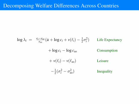
Decomposing Welfare Differences Across Countries

logλi = ei−euseus

(u + log ci + v(ì)− 12σ

2i ) Life Expectancy

+ log ci − log cus Consumption

+ v(ì)− v(ùs) Leisure

−12(σ2

i − σ2us) Inequality

As a ratio to per capita GDP

log λiyi

= ei−euseus

(u + log ci + v(`i)− 12σ

2i ) Life Expectancy

+ log ci/yi − log cus/yus Consumption Share


−12(σ2


Equivalent vs. Compensating Variation

What makes Rawls indifferent between the U.S. and country i?

Alternative answer:Scaling foreign consumption by some proportion λi.

V(eus, cus, `us, σus) = V(ei, ci/λi, `i, σi)

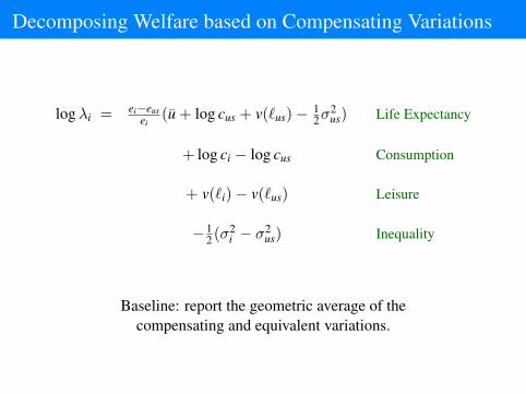
Decomposing Welfare based on Compensating Variations

logλi = ei−eusei

(u + log cus + v(`us)− 12σ

2us) Life Expectancy



−12(σ2


Baseline: report the geometric average of thecompensating and equivalent variations.

Decomposing Welfare Differences Across Time

logλt,t+1 =et+1−et

et+1(u + log ct + v(`t)− 1

2σ2t ) Life Expectancy

+ log ct+1 − log ct Consumption

+ v(`t+1)− v(`t) Leisure

−12(σ2

t+1 − σ2t ) Inequality

Baseline: report the geometric average of thecompensating and equivalent variations.

Data / Calibration for theMacro Calculations

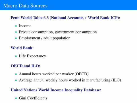
Macro Data Sources

Penn World Table 6.3 (National Accounts + World Bank ICP):

• Income• Private consumption, government consumption• Employment / adult population

World Bank:

• Life Expectancy

OECD and ILO:

• Annual hours worked per worker (OECD)• Average annual weekly hours worked in manufacturing (ILO)

United Nations World Income Inequality Database:

• Gini Coefficients

Leisure / Home Production

` = 1− annual hours worked per worker16× 365

· employmentadult population

.

• Annual hours worked per worker– SourceOECD has data for OECD countries (30 countries)– ILO has weekly hours worked in manufacturing for an additional

56 countries. Use regression to impute annual hours overall.– For remaining countries, just use average value based on income

above/below 0.5 × U.S. income

• Employment per adult population– From Penn World Tables and World Bank– Implicitly assumes kids and adults have same leisure/hp.

• Micro calculation uses hours per year from household surveys,varying across people.

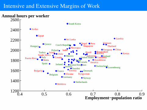
Intensive and Extensive Margins of Work

0.4 0.5 0.6 0.7 0.8 0.91200

1400

1600

1800

2000

2200

2400

2600

Austria

Belgium

Canada

Czech Republic

Denmark France

Germany

Greece Hungary

Iceland

Ireland

Italy Japan

South Korea

Luxembourg

Mexico

Netherlands

Norway

Poland

Spain

Sweden Switzerland

Turkey

United Kingdom

United States

Bangladesh Bolivia Brazil

Bulgaria

Chile

China

Colombia Croatia

Egypt

Estonia

Gambia

India

Indonesia

Israel

Jamaica

Jordan

Kazakhstan

Kenya

Kyrgyzstan

Malta

Moldova

Nepal

Nicaragua Paraguay

Peru

Puerto Rico

Singapore

South Africa

Sri Lanka

Thailand

Ukraine

Vietnam

Employment−population ratio

Annual hours per worker

Gini Coefficients and σ2

• When consumption is log normal, there’s a one-to-one mappingbetween the gini coefficient and the standard deviation:

G = 2Φ

(σ√2

)− 1

• G is the value of the Gini coefficient.

• Φ(·) is the cdf of the standard normal distribution.

• Invert to get σ

Within-Country Inequality

1/64 1/32 1/16 1/8 1/4 1/2 1 0.2

0.4

0.6

0.8

1

1.2

1.4

1.6

Albania

Bahamas

Bangladesh Belarus

Benin

Bolivia

Botswana

Brazil

Bulgaria

Burundi

Cambodia

Cameroon

Central African Republic

Chile China Colombia

Costa Rica Cote d‘Ivoire

Djibouti

Estonia

Ethiopia Georgia Ghana

Greece

Guinea−Bissau Haiti

Hong Kong

Iceland

India Israel

Jordan

Kenya

Latvia

Lesotho

Luxembourg

Malaysia Mauritania

Mauritius

Mexico

Moldova

Namibia

Niger Nigeria

Norway

Pakistan

Panama Puerto Rico

Singapore

Slovak Republic

Somalia

South Africa

Spain

Sweden

Tanzania Thailand Uganda

United Kingdom

United States Vietnam Yemen

Zambia

Zimbabwe

GDP per person

Standard deviation of log consumption

Hungary Japan

Calibrating the Utility from Leisure

• Assume v(`) = − θε1+ε(1− `)

1+εε

• Frisch elasticity of labor supply is ε– Hall (2009a,b) surveys/reports a Frisch elasticity of 0.7 for

intensive margin and 1.9 for both margins together.– We choose ε = 1 for our baseline — results not sensitive

• Using the standard F.O.C.:

u`/uc = w =⇒ θ = w(1− τ)(1− `)−1/ε/c

• For the U.S.:

c ≈ w(1− `), τ ≈ .387, ` ≈ .797 =⇒ θ ≈ 14.9

Calibrating the Intercept in Utility

Estimates of the value of remaining life for a U.S. 40-year old:

• Range from less than $2 million to more than $6 million.• See Murphy and Topel (2006), Ashenfelter and Greenstone

(2004), Viscusi and Aldy (2003), etc.

We calibrate to $4 million in our baseline case

• This requires u ≈ 5.54 if we normalize Cus,2000 = 1• Note: u raises the value of longevity relative to c, `.

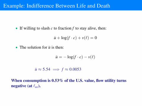
Example: Indifference Between Life and Death

• If willing to slash c to fraction f to stay alive, then:

u + log(f · c) + v(`) = 0

• The solution for u is then:

u = − log(f · c)− v(`)

u ≈ 5.54 =⇒ f ≈ 0.0053

When consumption is 0.53% of the U.S. value, flow utility turnsnegative (at `us).

Main Results

Key Point 1:

(a) GDP per person highly correlated with welfare across thebroad range of countries: 0.95.

(b) Nevertheless, differences are often important: typicaldeviation is 46%.

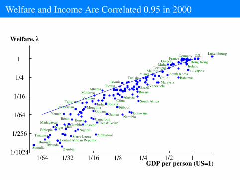
Welfare and Income Are Correlated 0.95 in 2000

1/64 1/32 1/16 1/8 1/4 1/2 1 1/1024

1/256

1/64

1/16

1/4

1

Albania

Algeria

Bahamas

Benin

Bolivia

Bosnia

Botswana

Brazil

Burundi

Cameroon


Chile

China

Cote d‘Ivoire

Djibouti

Ethiopia

France

Gambia

Germany

Greece

Guinea Guyana

Hong Kong

India

Ireland

Jordan

Kenya

South Korea

Lesotho

Luxembourg

Madagascar

Malaysia

Mali

Malta

Mauritius

Moldova

Mongolia

Namibia

Niger Nigeria

Poland

Portugal

Russia

Rwanda

Sierra Leone

Singapore

Somalia

South Africa Tajikistan

Tanzania

Tunisia

U.S.

Uzbekistan

Venezuela

Vietnam

Yemen

Zambia

Zimbabwe

GDP per person (US=1)

Welfare, λ

But Welfare typically differs from Income by about 46%

1/64 1/32 1/16 1/8 1/4 1/2 1 0

0.5

1

1.5

Albania

Armenia

Austria

Bahamas

Bangladesh

Belarus

Benin Bolivia

Bosnia

Botswana

Brazil

Bulgaria

Cambodia

Canada

Chile

China

Cote dIvoire

Croatia

Cyprus

Djibouti

Ecuador

Egypt

Ethiopia

France

Gambia

Georgia

Germany

Ghana

Greece

Guyana Haiti

Hong Kong

Hungary

Iceland

India Indonesia

Iran

Ireland

Japan

Jordan

Kenya

South Korea

Kyrgyzstan Luxembourg

Malaysia

Mali

Malta

Mauritius

Mexico

Moldova

Mongolia

Nepal

Nicaragua

Niger

Norway

Peru

Philippines

Portugal

Puerto Rico Romania

Russia

Rwanda

Senegal

Singapore

Slovenia

Somalia South Africa

Spain

Sweden

Tajikistan

Tanzania

Thailand Turkmenistan

U.K.

United States

Uzbekistan

Venezuela

Vietnam

Yemen

Zambia Zimbabwe


The ratio of Welfare to Income

Key Point 2: Western Europe is much closer to the U.S. when wetake into account Europe’s longer life expectancy, additionalleisure, and lower inequality.

U.S. vs. Western Europe in 2000

—— Decomposition ——Welfare Log Lifeλ Income Ratio Exp. C/Y Leis. Ineq.

U.S. 100 100 .000 .000 .000 .000 .000

France 97.4 70.1 .329 .119 -.055 .140 .125

• Western Europe’s high taxes and generous social safety net mayreduce work effort and GDP.

• But these programs have benefits that are not measured by GDP...

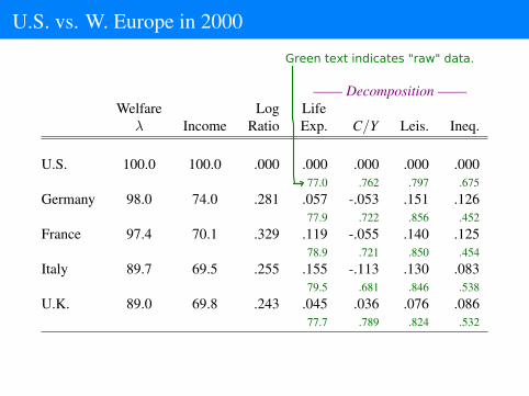
U.S. vs. W. Europe in 2000


U.S. 100.0 100.0 .000 .000 .000 .000 .00077.0 .762 .797 .675

Germany 98.0 74.0 .281 .057 -.053 .151 .12677.9 .722 .856 .452

France 97.4 70.1 .329 .119 -.055 .140 .12578.9 .721 .850 .454

Italy 89.7 69.5 .255 .155 -.113 .130 .08379.5 .681 .846 .538

U.K. 89.0 69.8 .243 .045 .036 .076 .08677.7 .789 .824 .532

+VIIR�XI\X�MRHMGEXIW��VE[��HEXE�

Key Point 3: Many developing countries are much poorer thanincomes suggest because of a combination of shorter lives andextreme inequality.

Welfare and Income, U.S. vs. Developed Asia in 2000


U.S. 100.0 100.0 .000 .000 .000 .000 .00077.0 .762 .797 .675

Japan 91.5 72.4 .235 .247 -.146 .025 .10881.1 .658 .806 .489

Hong Kong 90.0 82.1 .093 .236 -.064 -.008 -.07180.9 .714 .794 .772

Singapore 43.6 82.9 -.643 .060 -.581 -.106 -.01678.1 .426 .765 .698

South Korea 29.7 47.1 -.463 -.068 -.273 -.184 .06375.9 .580 .743 .574

C/Y: 71% in Hong Kong vs. 43% in Singapore

Welfare and Income, U.S. vs. Emerging Asia in 2000


U.S. 100.0 100.0 .000 .000 .000 .000 .00077.0 .762 .797 .675

Thailand 7.1 18.4 -.959 -.483 -.111 -.245 -.12068.3 .682 .728 .834

Indonesia 6.6 10.8 -.489 -.527 .057 -.050 .03167.5 .806 .781 .627

China 5.3 11.3 -.755 -.283 -.088 -.239 -.14571.4 .698 .729 .863

India 3.5 6.6 -.636 -.818 .148 -.009 .04362.5 .883 .794 .607

Welfare and Income, Other Emerging Markets in 2000


U.S. 100.0 100.0 .000 .000 .000 .000 .00077.0 .762 .797 .675

Mexico 17.4 25.9 -.397 -.173 -.018 .041 -.24774.0 .748 .811 .974

Brazil 12.2 21.8 -.584 -.380 .123 -.060 -.26670.4 .861 .778 .994

Russia 8.6 20.9 -.886 -.695 -.126 .005 -.06965.3 .672 .799 .771

Welfare and Income, Sub-Saharan Africa in 2000


U.S. 100.0 100.0 0.000 0.000 0.000 0.000 0.00077.0 .762 .797 .675

South Africa 4.4 21.6 -1.594 -1.376 0.122 0.083 -0.42356.1 .861 .826 1.140

Botswana 1.8 17.9 -2.292 -0.577 -0.171 0.028 -0.16748.9 .642 .807 .889

Malawi 0.4 2.9 -2.113 -1.952 0.254 -0.186 -0.22946.0 .982 .743 .956

South Africa: Life expectancy = 56 years⇒ factor of 4!

Key Point 4: Growth rates, 1980–2000

– Welfare: 2.5%– Income: 1.8%

Life expectancy adds more than 1.0%, except in Africa

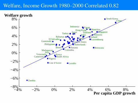
Welfare, Income Growth 1980–2000 Correlated 0.82

−4% −2% 0% 2% 4% 6% 8% −8%

−6%

−4%

−2%

0%

2%

4%

6%

8%

Bahamas

Botswana Brazil

Cameroon

China

Colombia

Cote d‘Ivoire

Egypt

El Salvador Guatemala

Hong Kong

India

Indonesia

Ireland

Japan

Kenya

South Korea

Lesotho

Luxembourg

Madagascar

Malaysia

Mauritius

Netherlands

Nigeria

Panama

Peru

Philippines

Singapore

South Africa

Spain

Thailand Turkey

United States

Venezuela

Zambia

Per capita GDP growth

Welfare growth

Welfare vs. Income Growth, 1980–2000

−4% −2% 0% 2% 4% 6% 8% −4%

−3%

−2%

−1%

0%

1%

2%

3%

Botswana

Brazil

Bulgaria

Cameroon China

Colombia

Cote d‘Ivoire

Denmark

Egypt

El Salvador France

Guatemala

Hong Kong

India

Indonesia

Ireland

Italy

Jamaica

Japan

Kenya

South Korea

Lesotho

Luxembourg

Madagascar

Malaysia

Mauritius Mexico

Nepal

Netherlands

Nigeria

Norway

Panama

Peru

Philippines

Singapore

South Africa

Spain Thailand

Tunisia

Turkey

U.S.

Venezuela

Zambia

Per capita GDP growth

Difference between Welfare and Income growth

Key Point 5: The mean absolute deviation between welfaregrowth and income growth is 0.99 percentage points.

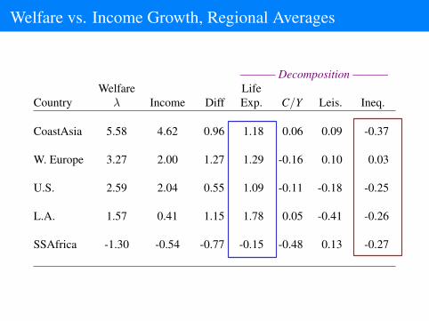
Welfare vs. Income Growth, Regional Averages

——— Decomposition ———Welfare Life

Country λ Income Diff Exp. C/Y Leis. Ineq.

CoastAsia 5.58 4.62 0.96 1.18 0.06 0.09 -0.37

W. Europe 3.27 2.00 1.27 1.29 -0.16 0.10 0.03

U.S. 2.59 2.04 0.55 1.09 -0.11 -0.18 -0.25

L.A. 1.57 0.41 1.15 1.78 0.05 -0.41 -0.26

SSAfrica -1.30 -0.54 -0.77 -0.15 -0.48 0.13 -0.27

Welfare vs. Income Growth, Growth Stars



S Korea 7.95 5.61 2.34 2.41 -0.74 0.51 0.1665.8, 75.9 .671, .580 .718, .743 .580, .522

China 7.13 6.81 0.32 0.83 -0.07 0.08 -0.5265.5, 71.4 .708, .698 .727, .731 .443, .637

H.K. 5.54 3.61 1.94 1.70 0.42 0.37 -0.5674.7, 80.9 .656, .714 .771, .794 .681, .829

Sing. 4.94 4.74 0.20 1.67 -0.91 -0.20 -0.3571.5, 78.1 .511, .426 .777, .766 .622, .726

India 4.03 2.89 1.14 1.25 0.12 0.10 -0.3255.7, 62.5 .862, .883 .788, .794 .565, .669

Welfare vs. Income Growth, U.S. and OECD



Japan 4.45 2.07 2.38 1.39 0.31 0.55 0.1376.1, 81.1 .618, .658 .771, .806 .543, .494

Italy 3.70 1.95 1.75 1.66 -0.09 0.13 0.0673.9, 79.5 .693, .681 .835, .846 .557, .536

France 3.60 1.61 1.98 1.44 -0.09 0.34 0.2974.2, 78.9 .734, .721 .822, .850 .560, .446

U.K. 3.32 2.19 1.13 1.25 -0.03 0.08 -0.1773.7, 77.7 .794, .789 .818, .824 .448, .520

U.S. 2.59 2.04 0.55 1.09 -0.11 -0.18 -0.2573.7, 77.0 .778, .762 .809, .797 .601, .680

Welfare vs. Income Growth, Developing Countries



Mexico 1.83 0.53 1.30 1.81 -0.01 -0.32 -0.1966.8, 74.0 .749, .748 .835, .811 .827, .871

Brazil 1.76 0.18 1.59 1.88 0.23 -0.44 -0.0862.8, 70.4 .822, .861 .796, .769 .957, .973

Botswa. 1.20 4.35 -3.16 -2.72 -0.88 0.29 0.1660.5, 48.9 .766, .642 .783, .801 .906, .871

SAfrica -0.89 0.10 -0.99 -0.32 0.14 0.15 -0.9657.2, 56.1 .837, .861 .807, .818 .762, .981

Robustness Checks

Robustness

Key Points are all qualitatively robust.

Sensitivity of magnitudes in order of importance:

• CV versus EV• u — U.S. value of life• K/Y: current level versus steady state• Coefficient of relative risk aversion• Parameterization of utility from leisure

Robustness — Summary Results

# of countries— Median absolute deviation — with negative

Robustness check Levels Growth rate flow utility

Benchmark case 0.379 0.99 0

Equivalent variation 0.269 0.93 0Compensating variation 0.442 1.03 0γ = 1.5, c = 0 0.329 0.61 52γ = 1.5, c = .088 0.386 0.86 6γ = 2.0, c = .271 0.414 0.96 6θ from FOC for France 0.413 1.05 0Frisch elasticity = 1.9 0.383 0.98 0Value of Life = $3m 0.286 0.73 14Value of Life = $5m 0.464 1.39 0

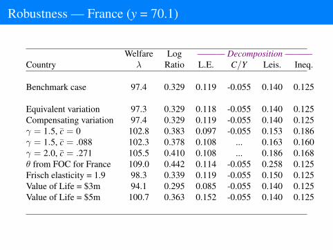
Robustness — France (y = 70.1)

Welfare Log ——— Decomposition ———Country λ Ratio L.E. C/Y Leis. Ineq.

Benchmark case 97.4 0.329 0.119 -0.055 0.140 0.125

Equivalent variation 97.3 0.329 0.118 -0.055 0.140 0.125Compensating variation 97.4 0.329 0.119 -0.055 0.140 0.125γ = 1.5, c = 0 102.8 0.383 0.097 -0.055 0.153 0.186γ = 1.5, c = .088 102.3 0.378 0.108 ... 0.163 0.160γ = 2.0, c = .271 105.5 0.410 0.108 ... 0.186 0.168θ from FOC for France 109.0 0.442 0.114 -0.055 0.258 0.125Frisch elasticity = 1.9 98.3 0.339 0.119 -0.055 0.150 0.125Value of Life = $3m 94.1 0.295 0.085 -0.055 0.140 0.125Value of Life = $5m 100.7 0.363 0.152 -0.055 0.140 0.125

Baseline Welfare Measure, 2000

1/64 1/32 1/16 1/8 1/4 1/2 1 1/1024

1/256

1/64

1/16

1/4

1

Albania

Algeria

Bahamas

Benin

Bolivia

Bosnia

Botswana

Brazil

Burundi

Cameroon


Chile

China

Cote d‘Ivoire

Djibouti

Ethiopia

France

Gambia

Germany

Greece

Guinea Guyana

Hong Kong

India

Ireland

Jordan

Kenya

South Korea

Lesotho

Luxembourg

Madagascar

Malaysia

Mali

Malta

Mauritius

Moldova

Mongolia

Namibia

Niger Nigeria

Poland

Portugal

Russia

Rwanda

Sierra Leone

Singapore

Somalia

South Africa Tajikistan

Tanzania

Tunisia

U.S.

Uzbekistan

Venezuela

Vietnam

Yemen

Zambia

Zimbabwe


Welfare, λ

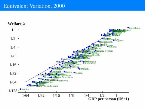
Equivalent Variation, 2000

1/64 1/32 1/16 1/8 1/4 1/2 1 1/128

1/64

1/32

1/16

1/8

1/4

1/2

1

Albania

Algeria

Armenia

Australia Austria

Azerbaijan

Bahamas

Bangladesh

Belarus

Belgium

Benin

Bolivia

Bosnia and Herzegovina

Botswana

Brazil

Bulgaria

Burkina Faso

Burundi

Cambodia Cameroon

Canada


Chile

China

Colombia

Costa Rica

Cote d‘Ivoire

Croatia

Cyprus

Czech Republic

Denmark

Djibouti

Dominican Republic

Ecuador Egypt El Salvador

Estonia

Ethiopia

Fiji

Finland

France

Gambia

Georgia

Germany

Ghana

Greece

Guatemala

Guinea

Guinea−Bissau

Guyana Haiti

Honduras

Hong Kong

Hungary

Iceland

India

Indonesia

Iran

Ireland Israel

Italy

Jamaica

Japan

Jordan Kazakhstan

Kenya

South Korea

Kyrgyzstan

Laos

Latvia

Lesotho

Lithuania

Luxembourg

Macedonia

Madagascar Malawi

Malaysia

Mali

Malta

Mauritania

Mauritius

Mexico

Moldova

Mongolia

Mozambique

Namibia Nepal

Netherlands

New Zealand

Nicaragua

Niger Nigeria

Norway

Pakistan

Panama

Papua New Guinea

Paraguay Peru Philippines

Poland

Portugal Puerto Rico

Romania

Russia

Rwanda

Senegal

Sierra Leone

Singapore

Slovak Republic

Slovenia

Somalia

South Africa

Spain

Sri Lanka

Swaziland

Sweden Switzerland

Tajikistan

Tanzania

Thailand

Trinidad &Tobago Tunisia

Turkey

Turkmenistan

Uganda

Ukraine

United Kingdom United States

Uzbekistan

Venezuela

Vietnam

Yemen

Zambia

Zimbabwe


Welfare, λ

Compensating Variation, 2000

1/64 1/32 1/16 1/8 1/4 1/2 1

1/4096

1/1024

1/256

1/64

1/16

1/4

1

Albania

Algeria

Armenia

Australia Austria

Azerbaijan

Bahamas

Bangladesh

Belarus

Belgium

Benin

Bolivia

Bosnia and Herzegovina

Botswana

Brazil Bulgaria

Burkina Faso

Burundi

Cambodia Cameroon

Canada


Chile

China

Colombia

Costa Rica

Cote d‘Ivoire

Croatia

Cyprus

Czech Republic

Denmark

Djibouti

Dominican Republic Ecuador Egypt El Salvador

Estonia

Ethiopia

Fiji

Finland France

Gambia

Georgia

Germany

Ghana

Greece

Guatemala

Guinea

Guinea−Bissau

Guyana

Haiti

Honduras

Hong Kong

Hungary

Iceland

India

Indonesia

Iran

Ireland Israel Italy

Jamaica

Japan

Jordan Kazakhstan

Kenya

South Korea

Kyrgyzstan

Laos

Latvia

Lesotho

Lithuania

Luxembourg

Macedonia

Madagascar

Malawi

Malaysia

Mali

Malta

Mauritania

Mauritius

Mexico

Moldova

Mongolia

Mozambique

Namibia Nepal

Netherlands New Zealand

Nicaragua

Niger

Nigeria

Norway

Pakistan

Panama

Papua New Guinea

Paraguay Peru Philippines

Poland

Portugal Puerto Rico

Romania

Russia

Rwanda

Senegal

Sierra Leone

Singapore Slovak Republic

Slovenia

Somalia

South Africa

Spain

Sri Lanka

Swaziland

Sweden Switzerland

Tajikistan

Tanzania

Thailand

Trinidad &Tobago Tunisia

Turkey

Turkmenistan

Uganda

Ukraine

United Kingdom United States

Uzbekistan

Venezuela

Vietnam

Yemen

Zambia

Zimbabwe


Welfare, λ

Adjusting the Consumption Share for Transition Dynamics

0.2 0.4 0.6 0.8 10.1

0.2

0.3

0.4

0.5

0.6

0.7

0.8

0.9

1

Algeria

Bahamas

Bangladesh

Bolivia

Botswana

Brazil

Bulgaria

Burundi Cameroon

China Colombia

Costa Rica

Djibouti

Ethiopia Gambia

Germany

Ghana

Greece

Guatemala

Guinea

Guyana

Haiti

India

Iraq

Ireland

Japan

South Korea Luxembourg

Madagascar

Malawi

Malaysia

Mauritania

Mauritius

Mongolia

Nepal

Norway

Paraguay Philippines

Portugal

Romania

Rwanda

Senegal Sierra Leone

Singapore

Somalia

South Africa

Sweden

Thailand

United States

Venezuela

Vietnam

Zimbabwe

C / Y

(C / Y)ss

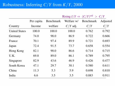
Robustness: Inferring C/Y from K/Y , 2000

Rising I/Y ⇒ (C/Y)adj > C/YPer capita Benchmark Welfare w/ Benchmark Adjusted

Country Income welfare C/Y adj. C/Y C/Y

United States 100.0 100.0 100.0 0.762 0.792

Germany 74.0 98.0 86.9 0.722 0.666

France 70.1 97.4 89.9 0.721 0.693

Japan 72.4 91.5 73.7 0.658 0.554

Hong Kong 82.1 90.0 86.6 0.714 0.715

U.K. 69.8 89.0 86.1 0.789 0.795

Singapore 82.9 43.6 46.9 0.426 0.477

South Korea 47.1 29.7 30.1 0.580 0.611

China 11.3 5.3 5.9 0.698 0.810

India 6.6 3.5 3.5 0.883 0.911

Micro Calculations

Micro Calculations

Household Surveys for various country-years

• Household expenditures

• Age, Hours Worked of each household member

Have analyzed micro data for:

• U.S. (1984–2006)

• France(1984–2005)

• India (1984-2005)

• Mexico(1984-2002)

• South Africa(1993)

10 Advantages to Micro Calculations

• Make sure consumption (not income) inequality

• Allow arbitrary (non-normal) distribution of consumption

• Drop durables (lumpy)

• Individual (rather than household) consumption

• Better measure of hours worked if non-OECD

• Incorporate inequality in leisure

• Adjust for age composition of population

• Incorporate survival rates by age

• Uniform use of sampling weights

• Allow government consumption to lower inequality (if desired)

Theory for the Micro Calculation

• Basic notation:a ≡ agej ≡ people within age groupSi

a ≡ Probability of surviving to age a in country i

• Mortality notation

susa ≡

Susa∑

a Susa

∆sia ≡

Sia − Sus

a∑a Sus

a

• Demographically-adjusted averages:

ci ≡∑

a

susa

∑j

ωijaci

ja

¯i ≡∑

a

susa

∑j

ωija`

ija

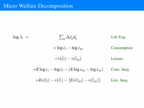
Micro Welfare Decomposition

logλi =∑

a ∆siaui

a Life Exp.


+v(¯i)− v(¯us) Leisure

+E log ci − log ci − (E log cus − log cus) Cons. Ineq.

+Ev(`i)− v(¯i)−(Ev(`us)− v(¯us)

)Leis. Ineq.

Micro Calculations: Levels

—— Decomposition ——Welfare Log Life Cons Leisλ Income Ratio Exp. C/Y Leis. Ineq Ineq

France 103.8 68.7 .413 .132 -.088 .117 .116 .135(macro) 97.4 70.1 .329 .119 -.055 .140 .125 ...

India 4.9 8.0 -.487 -.614 .102 .002 .050 -.027(macro) 3.5 6.6 -.636 -.818 .148 .009 .043 ...

Mexico 18.7 25.7 -.319 -.146 -.013 .019 -.170 -.010(macro) 17.4 25.9 -.397 -.173 -.018 .041 -.247 ...

S Africa 8.5 22.6 -.744 -.609 .217 .084 -.427 -.008(macro) 4.4 21.6 -1.594 -1.376 .122 .083 -.423 ...

Micro Calculations: Growth Rates

—— Decomposition ——Welfare Income Life Cons. Leis.Growth Growth Diff Exp. C/Y Leis. Ineq. Ineq

France 2.46 1.64 0.82 .91 -.10 -.02 .00 .03(macro) 3.60 1.61 1.98 1.44 -.09 .34 .29 ...

India 3.69 3.68 .01 .52 -.38 .02 -.17 .01(macro) 3.11 2.89 .22 .48 .12 -.06 -.32 ...

Mexico 1.24 0.83 .41 .78 -.13 -.08 -.24 -.07(macro) 0.61 0.53 .08 1.14 -.01 -.87 -.19 ...

U.S. 2.39 1.94 .45 .70 .00 -.33 -.01 .09(macro) 2.08 2.04 .05 .76 -.11 -.36 -.25 ...

Conclusions

• Income and welfare are highly correlated in both levels andgrowth rates.

• Nevertheless, differences between income and welfare are ofteneconomically important:

– Western Europe looks much closer to U.S. living standards.

– Most other countries are further behind, primarily due to lowerlife expectancy.

– Longer lives add over one percentage point, on average, towelfare growth per year 1980–2000.

beyond gdp? welfare across countries and timeklenow.com/jones_klenow_slides.pdfbeyond gdp? welfare...

Documents