biodiversity increases and decreases ecosystem stability
TRANSCRIPT
HAL Id: hal-01944370https://hal.umontpellier.fr/hal-01944370
Submitted on 12 Dec 2018
HAL is a multi-disciplinary open accessarchive for the deposit and dissemination of sci-entific research documents, whether they are pub-lished or not. The documents may come fromteaching and research institutions in France orabroad, or from public or private research centers.
L’archive ouverte pluridisciplinaire HAL, estdestinée au dépôt et à la diffusion de documentsscientifiques de niveau recherche, publiés ou non,émanant des établissements d’enseignement et derecherche français ou étrangers, des laboratoirespublics ou privés.
Biodiversity increases and decreases ecosystem stabilityFrank Pennekamp, Mikael Pontarp, Andrea Tabi, Florian Altermatt, RomanAlther, Yves Choffat, Emanuel A Fronhofer, Pravin Ganesanandamoorthy,
Aurélie Garnier, Jason Griffiths, et al.
To cite this version:Frank Pennekamp, Mikael Pontarp, Andrea Tabi, Florian Altermatt, Roman Alther, et al.. Biodiver-sity increases and decreases ecosystem stability. Nature, Nature Publishing Group, 2018, 563 (7729),pp.109-112. �10.1038/s41586-018-0627-8�. �hal-01944370�
1
Biodiversity increases and decreases 1
ecosystem stability 2 3 Frank Pennekampa - email: [email protected] 4 Mikael Pontarpa, b - [email protected] 5 Andrea Tabia - [email protected] 6 Florian Altermatta,c - [email protected] 7 Roman Althera,c – [email protected] 8 Yves Choffata - [email protected] 9 Emanuel A. Fronhofera,c,g – [email protected] 10 Pravin Ganesanandamoorthya, c – [email protected] 11 Aurélie Garniera - [email protected] 12 Jason I. Griffithsf - [email protected] 13 Suzanne Greenea,e - [email protected] 14 Katherine Horgana – [email protected] 15 Thomas M. Massiea - [email protected] 16 Elvira Mächlera,c - [email protected] 17 Gian-Marco Palamaraa,h - [email protected] 18 Mathew Seymourc, d - [email protected] 19 Owen L. Petcheya - email: [email protected] 20 21 Affiliations: 22 aDepartment of Evolutionary Biology and Environmental Studies, University of Zurich, 23 Winterthurerstrasse 190, 8057 Zurich, Switzerland 24 bDepartment of Ecology and Environmental Science, Umeå University, 90187 Umeå, 25 Sweden 26 cDepartment of Aquatic Ecology, Eawag: Swiss Federal Institute of Aquatic Science and 27 Technology, Überlandstrasse 133, 8600 Dübendorf, Switzerland 28 fDepartment of Mathematics, University of Utah, Salt Lake City, UT, 84112,USA 29 30 Present addresses: 31 dMolecular Ecology and Fisheries Genetics Laboratory, School of Biological Sciences, 32 Environment Centre Wales Building, Bangor University, Bangor, Gwynedd, UK 33 eMassachusetts Institute of Technology, 77 Massachusetts Avenue, Cambridge, MA USA 34 gISEM, Université de Montpellier, CNRS, IRD, EPHE, Montpellier, France 35 hDepartment Systems Analysis, Integrated Assessment and Modelling, Eawag: Swiss Federal 36 Institute of Aquatic Science and Technology, Überlandstrasse 133, 8600 Dübendorf, 37 Switzerland 38 39 This is a post-peer-review, pre-copyedit version of an article published in Nature. 40 The final authenticated version is available online at: 41 https://doi.org/10.1038/s41586-018-0627-8 42 43 44
2
Losses and gains in species diversity affect ecological stability1–7 and the sustainability 45 of ecosystem functions and services8–13. Experiments and models reveal positive, 46 negative, and no effects of diversity on individual components of stability such as 47 temporal variability, resistance, and resilience2,3,6,11,12,14. How these stability components 48 covary is poorly appreciated15, as are diversity effects on overall ecosystem stability16, 49 conceptually akin to ecosystem multifunctionality17,18. We observed how temporal 50 variability, resistance, and overall ecosystem stability responded to diversity (i.e. species 51 richness) in a large experiment involving 690 micro-ecosystems sampled 19 times over 52 40 days, resulting in 12939 samplings. Species richness increased temporal stability but 53 decreased resistance to warming. Thus, two stability components negatively covaried 54 along the diversity gradient. Previous biodiversity manipulation studies rarely reported 55 such negative covariation despite general predictions of negative effects of diversity on 56 individual stability components3. Integrating our findings with the ecosystem 57 multifunctionality concept revealed hump- and U-shaped effects of diversity on overall 58 ecosystem stability. That is, biodiversity can increase overall ecosystem stability when 59 biodiversity is low, and decrease it when biodiversity is high, or the opposite with a U-60 shaped relationship. Effects of diversity on ecosystem multifunctionality would also be 61 hump- or U-shaped if diversity has positive effects on some functions and negative 62 effects on others. Linking the ecosystem multifunctionality concept and ecosystem 63 stability can transform perceived effects of diversity on ecological stability and may 64 assist translation of this science into policy-relevant information. 65 66 Ecological stability consists of numerous components including temporal variability, 67 resistance to environmental change, and rate of recovery from disturbance1,2,16. Effects of 68 species losses and gains on these components are of considerable interest, not least due to 69 potential effects on ecosystem functioning and hence the sustainable delivery of ecosystem 70 services1–13. A growing number of experimental studies reveal stabilising effects of diversity 71 on individual stability components. In particular, higher diversity often, but not always, 72 reduces temporal variability of biomass production13. Positive effects of diversity on 73 resistance are common, though neutral and negative effects on resistance and resilience also 74 occur9,13,19,20. While assessment of individual stability components is essential, a more 75 integrative approach to ecological stability could lead to clearer conceptual understanding15 76 and might improve policy guidance concerning ecological stability16. 77
Analogous to ecosystem multifunctionality17,18, a more integrative approach considers 78 variation in multiple stability components, and the often-ignored covariation among stability 79 components. The nature of this covariation is of paramount importance, as it defines whether 80 diversity has consistent effects on multiple stability components, or whether some stability 81 components increase with diversity while others decrease. Surprisingly, the nature, 82 prevalence, and implications of negative covariation between stability components along 83 diversity gradients are almost completely overlooked, including the ensuing possibility for 84 non-monotonic effects of diversity on overall ecosystem stability. 85
We first describe new experimental findings of how biodiversity affects the intrinsic 86 stability of ecosystems and their resistance to warming. Temperature is a highly relevant 87 disturbance due to its importance for biological processes and its great variability through 88 space and time. However, our findings equally apply to and have implications for other 89 environmental changes that could result in opposing effects on stability components such as 90 flooding12 or chemical stress21. We then review other evidence for negative covariation in 91 effects of diversity on stability and potential mechanisms. Finally, we analyse overall 92 ecosystem stability, a concept that embraces the covariation between stability components 93 and their weighting, and show the plausibility of previously overlooked non-monotonic 94 (hump- and U-shaped) effects of diversity on overall ecosystem stability. 95
3
We performed a factorial manipulation of the diversity and composition of competing 96 species (1 to 6 species, 53 unique community compositions) and temperature (six constant 97 levels, modelled as a linear predictor) in microbial communities of bacterial consumers, and 98 recorded community biomass dynamics over time. For each replicate we then calculated two 99 stability components: resistance (= [total biomass at T˚C – total biomass at 15˚C] / [T˚C – 100 15˚C] where T is the temperature of the replicate) and the temporal stability of biomass 101 (inverse of coefficient of variation of community biomass). While these stability indices are 102 widely used by empiricists, they should not be mistaken for mathematical definitions such as 103 asymptotic resilience, which are more precise but also more restrictive22. 104
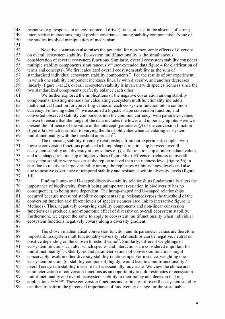
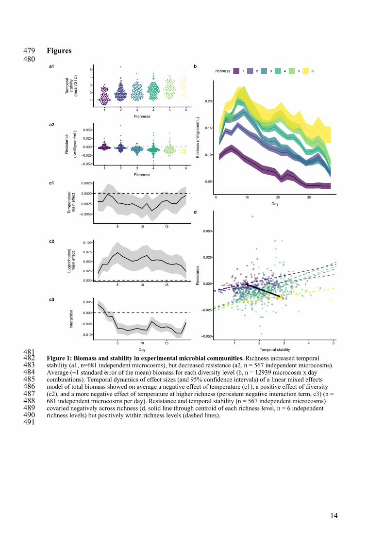
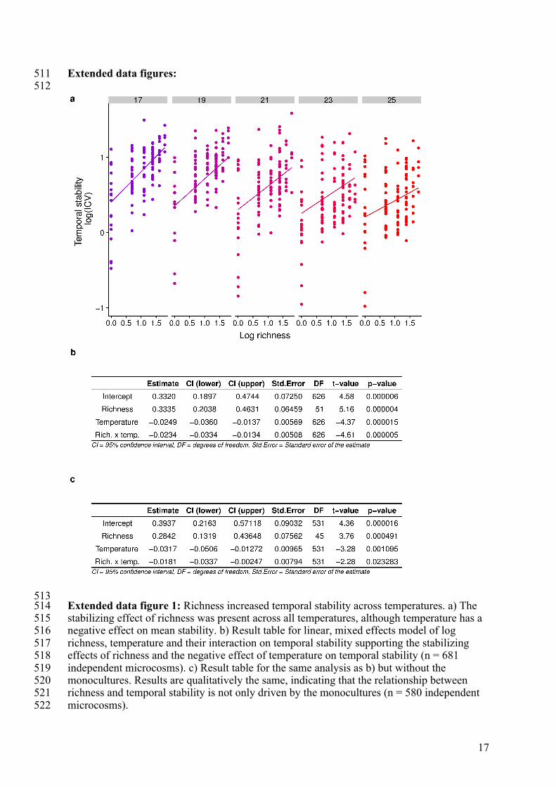
Increased species richness caused greater temporal stability of total biomass (figure 1-105 a1) (linear mixed model of log inverse CV: richness effect size 0.33 with a standard error of 106 0.065) at all temperatures (extended data figure 1). Total biomass increased during the first 107 week of the experiment and then declined over the next five weeks and total biomass was 108 higher in more species-rich communities (figure 1-b, 1-c2, extended data table 1) (effect size 109 for log richness 0.05 [units of mg/mL/log(species richness) unit] with 0.0096 standard error). 110
In contrast, increased species richness decreased resistance of total biomass to 111 warming (figure 1-a2) (negative effect of log richness in a linear model, effect size of -0.006 112 [mg/°C/ log(species richness) unit] with a standard error of 0.0018). Richness negatively 113 affected resistance measured on both absolute and relative scales (extended data figure 2). 114 This effect was corroborated in analyses of total biomass by a negative interaction term 115 between temperature and richness, which persisted through the experiment except during the 116 first days (figure 1-c3) (log(richness) x temperature interaction of -0.0053 [units of 117 mg/mL/°C/log(species richness) unit] with standard error of 0.00051) despite large variation 118 in dynamics of total biomass (figure 1-b). This negative interaction reflects a stronger 119 negative effect of temperature on total biomass (i.e. lower resistance) in richer communities 120 (i.e. a richness-dependent response of total biomass to temperature). 121 Hence, temporal stability and resistance were negatively correlated across the species 122 richness gradient (figure 1-d, RMA analysis with slope = -0.009, 95% CI = -0.0178 to -123 0.0051). Niche complementarity, statistical averaging, low overall response diversity, and 124 possibly lower response diversity in more diverse communities were likely causes of the 125 opposite effects of richness on temporal stability (extended data figure 3). The two stability 126 components were, however, positively correlated within any single level of species richness 127 (figure 1-d, extended data table 2). That is, composition variation without changes in species 128 richness resulted in positively covarying temporal stability and resistance. 129
130 Next, we examined studies (including our own) measuring multiple stability 131
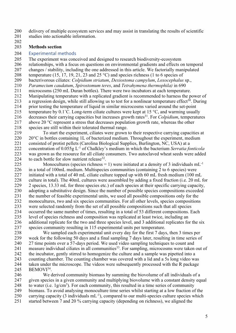
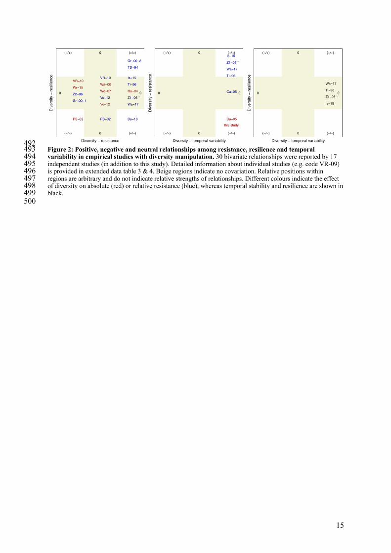
components across diversity gradients based on a review by Donohue et al. (2016)16 (figure 132 2, extended data table 3 & 4). Seven of 30 comparisons show positive covariance, twenty 133 show no covariance, and three showed negative covariance. Our study for the first time 134 identifies negative covariation between resistance and temporal variability caused by intrinsic 135 dynamics only. Although infrequently reported, negative covariation is disproportionately 136 important because it complicates conclusions about and practical implications of effects of 137 diversity on stability. Furthermore, these studies may be unrepresentative of the true 138 prevalence of negative covariation, due to it being overlooked, publication bias towards 139 positive diversity-stability relationships3 or if the scale of analysis masks such covariation, 140 e.g. within richness versus across richness. 141
A general mechanistic understanding of why different studies find different 142 correlations would be a major step forward. Of the 30 pairs of stability components, only 143 seven were accompanied by quantitative analyses of mechanism for both diversity-stability 144 relationships (extended data table 4). Response diversity was implicated in five of these 145 seven. Indeed, response diversity has been identified as an important driver of the resilience 146 of ecological systems23,24, and correlation among effect (i.e. high biomass production) and 147
4
response (e.g. response to an environmental driver) traits, at least in the absence of strong 148 interspecific interactions, might predict covariance among stability components23. None of 149 the studies involved manipulation of mechanism. 150 151
Negative covariation also raises the potential for non-monotonic effects of diversity 152 on overall ecosystem stability. Ecosystem multifunctionality is the simultaneous 153 consideration of several ecosystem functions. Similarly, overall ecosystem stability considers 154 multiple stability components simultaneously16 (see extended data figure 4 for clarification of 155 terms and concepts). We first calculated overall ecosystem stability as the sum of 156 standardised individual ecosystem stability components25. For the results of our experiment, 157 in which one stability component increases linearly with diversity, and another decreases 158 linearly (figure 1-a1,2), overall ecosystem stability is invariant with species richness since the 159 two standardized components perfectly balance each other. 160
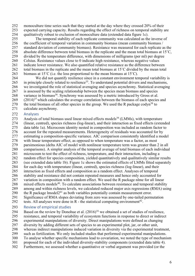
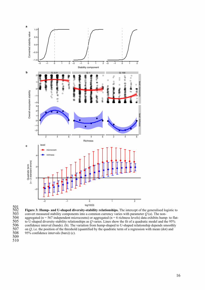
We further explored the implications of the negative covariation among stability 161 components. Existing methods for calculating ecosystem multifunctionality include a 162 mathematical function for converting values of each ecosystem function into a common 163 currency. Following others26, we assumed a logistic shape conversion function, and 164 converted observed stability components into the common currency, with parameter values 165 chosen to ensure that the range of the data includes the lower and upper asymptote. Here we 166 present the influence of the value of the intercept (parameter Q) of the conversion function 167 (figure 3a), which is similar to varying the threshold value when calculating ecosystem 168 multifunctionality with the threshold approach27. 169
The opposing stability-diversity relationships from our experiment, coupled with 170 logistic conversion functions produced a hump-shaped relationship between overall 171 ecosystem stability and diversity at low values of Q, a flat relationship at intermediate values, 172 and a U-shaped relationship at higher values (figure 3b,c). Effects of richness on overall 173 ecosystem stability were weaker at the replicate level than the richness level (figure 3b) in 174 part due to relatively large variability among the replicates within richness levels and also 175 due to positive covariance of temporal stability and resistance within diversity levels (figure 176 1d). 177
Finding hump- and U-shaped diversity-stability relationships fundamentally alters the 178 importance of biodiversity, from it being unimportant (variation in biodiversity has no 179 consequence), to being state dependent. The hump-shaped and U-shaped relationships 180 occurred because measured stability components (e.g. resistance) cross the threshold of the 181 conversion function at different levels of species richness (see link to interactive figure in 182 Methods). Thus, negatively covarying stability components and non-linear conversion 183 functions can produce a non-monotonic effect of diversity on overall ecosystem stability. 184 Furthermore, we expect the same to apply to ecosystem multifunctionality when individual 185 ecosystem functions negatively covary along a diversity gradient. 186
187 The chosen mathematical conversion function and its parameter values are therefore 188 important. Ecosystem multifunctionality-diversity relationships can be negative, neutral or 189 positive depending on the chosen threshold value27. Similarly, different weightings of 190 ecosystem functions can alter which species and interactions are considered important for 191 multifunctionality26. Other types and parameterisations of conversion functions might 192 conceivably result in other diversity-stability relationships. For instance, weighting one 193 ecosystem function (or stability component) highly, would lead to a multifunctionality / 194 overall ecosystem stability measure that is essentially univariate. We view the choice and 195 parameterization of conversion functions as an opportunity to tailor estimates of ecosystem 196 multifunctionality and overall ecosystem stability to their policy and decision making 197 applications16,26,28,29. These conversion functions and estimates of overall ecosystem stability 198 can then transform the perceived importance of biodiversity change for the sustainable 199
5
delivery of multiple ecosystem services and may assist in translating the results of scientific 200 studies into actionable information. 201 202 Methods section 203 Experimental methods 204 The experiment was conceived and designed to research biodiversity-ecosystem 205 relationships, with a focus on questions on environmental gradients and effects on temporal 206 changes / stability, including the one addressed in this article. We factorially manipulated 207 temperature (15, 17, 19, 21, 23 and 25 °C) and species richness (1 to 6 species of 208 bacterivorous ciliates: Colpidium striatum, Dexiostoma campylum, Loxocephalus sp., 209 Paramecium caudatum, Spirostomum teres, and Tetrahymena thermophila) in 690 210 microcosms (250 mL Duran bottles). There were two incubators at each temperature. 211 Manipulating temperature with a replicated gradient is recommended to harness the power of 212 a regression design, while still allowing us to test for a nonlinear temperature effect30. During 213 prior testing the temperature of liquid in similar microcosms varied around the set-point 214 temperature by 0.1˚C. Long-term ciliate cultures were kept at 15 °C, and warming usually 215 decreases their carrying capacities but increases growth rates31. For Colpidium, temperatures 216 above 20 °C represent a stress that decreases population growth rate, whereas the other 217 species are still within their tolerated thermal range. 218
To start the experiment, ciliates were grown to their respective carrying capacities at 219 20°C in bottles containing 1L of bacterized medium. Throughout the experiment, medium 220 consisted of protist pellets (Carolina Biological Supplies, Burlington, NC, USA) at a 221 concentration of 0.055g L-1 of Chalkley’s medium in which the bacterium Serratia fonticola 222 was grown as the resource for all ciliate consumers. Two autoclaved wheat seeds were added 223 to each bottle for slow nutrient release32. 224
Monocultures (species richness = 1) were initiated at a density of 3 individuals mL-1 225 in a total of 100mL medium. Multispecies communities (containing 2 to 6 species) were 226 initiated with a total of 40 mL ciliate culture topped up with 60 mL fresh medium (100 mL 227 culture in total). The 40mL cultures were assembled by adding a fixed fraction (i.e. 20 mL for 228 2 species, 13.33 mL for three species etc.) of each species at their specific carrying capacity, 229 adopting a substitutive design. Since the number of possible species compositions exceeded 230 the number of feasible experimental units, we used all possible compositions only for the 231 monocultures, two and six species communities. For all other levels, species compositions 232 were selected randomly from the set of all possible compositions such that all species 233 occurred the same number of times, resulting in a total of 53 different compositions. Each 234 level of species richness and composition was replicated at least twice, including an 235 additional replicate for the two and three species level, and 3 additional replicates for the six 236 species community resulting in 115 experimental units per temperature. 237
We sampled each experimental unit every day for the first 7 days, then 3 times per 238 week for the following 50 days and a final sampling 7 days later, resulting in time series of 239 27 time points over a 57-days period. We used video sampling techniques to count and 240 measure individual ciliates in all communities33. For sampling, microcosms were taken out of 241 the incubator, gently stirred to homogenize the culture and a sample was pipetted into a 242 counting chamber. The counting chamber was covered with a lid and a 5s long video was 243 taken under the microscope. The videos were subsequently processed with the R package 244 BEMOVI34. 245
We derived community biomass by summing the biovolume of all individuals of a 246 given species in a given community and multiplying biovolume with a constant density equal 247 to water (i.e. 1g/cm3). For each community, this resulted in a time series of community 248 biomass. To avoid analysing monoculture time series whilst starting at a low fraction of the 249 carrying capacity (3 individuals mL-1), compared to our multi-species culture species which 250 started between 7 and 20 % carrying capacity (depending on richness), we aligned the 251
6
monoculture time series such that they started at the day where they crossed 20% of their 252 expected carrying capacity. Results regarding the effect of richness on temporal stability are 253 qualitatively robust to exclusion of monoculture data (extended data figure 1c). 254 The temporal stability of each replicate community was calculated as the inverse of 255 the coefficient of temporal variation in community biomass (mean community biomass / 256 standard deviation of community biomass). Resistance was measured for each replicate as the 257 absolute difference between total biomass in the replicate and the mean total biomass at 15˚C, 258 divided by the temperature difference, with dimensions of milligrams (per ml) per degree 259 Celsius. Resistance values close to 0 indicate high resistance, whereas negative values 260 indicate lower resistance. We also quantified relative resistance as the difference between 261 total biomass in the replicate and the mean total biomass at 15˚C divided by the mean total 262 biomass at 15˚C (i.e. the loss proportional to the mean biomass at 15˚C). 263
We did not quantify resilience since in a constant environment temporal variability is 264 in principle closely related to resilience35. To understand potential drivers and mechanisms, 265 we investigated the role of statistical averaging and species asynchrony. Statistical averaging 266 is assessed by the scaling relationship between the species mean biomass and species 267 variance in biomass36. Synchrony was assessed by a metric introduced by Gross et al. 268 (2014)37 which calculates the average correlation between the biomass of each species and 269 the total biomass of all other species in the group. We used the R package codyn38 to 270 calculate asynchrony. 271 Analyses 272 Analysis of total biomass used linear mixed effects models39 (LMMs), with temperature 273 (linear, centred), species richness (log-linear), and their interaction as fixed effects (extended 274 data table 1a). Microcosm identity nested in composition was included as random factor to 275 account for the repeated measurements. Heterogeneity of residuals was accounted for by 276 estimating a composition-specific variance. AIC comparison consistently identified a model 277 with linear temperature effect, as opposed to when temperature was a factor, as most 278 parsimonious (delta AIC of model with nonlinear temperature term was greater than 2 in all 279 comparisons). A simpler analysis of the temporal average of total biomass of each individual 280 microcosm to test the effect of richness, temperature, and their interaction, including a 281 random effect for species composition, yielded quantitatively and qualitatively similar results 282 (see extended data table 1b). Figure 1c shows the estimated effects of LMMs fitted separately 283 for each day with temperature (linear, centred), species richness (log-linear), and their 284 interaction as fixed effects and composition as a random effect. Analyses of temporal 285 stability and resistance did not contain repeated measures and hence only accounted for 286 variation in composition with a random effect. We used the R package nlme for all linear 287 mixed effects models40. To calculate associations between resistance and temporal stability 288 among and within richness levels, we calculated reduced major axis regressions (RMA) using 289 the R package lmodel241 as both variables potentially contain measurement error. 290 Significance of RMA slopes deviating from zero was assessed by one-tailed permutation 291 tests. All analyses were done in R - the statistical computing environment42. 292 Review of empirical studies 293 Based on the review by Donohue et al. (2016)16 we obtained a set of studies of resilience, 294 resistance, and temporal variability of ecosystem functions in response to direct or indirect 295 experimental manipulations of diversity. Direct manipulations were defined as changing 296 diversity by adding different sets of species to an experimental plot, jar, or other unit, 297 whereas indirect manipulations induced variation in diversity via the experimental treatment, 298 such as fertilization. We only included studies that performed experimental manipulations. 299 To analyse whether specific mechanisms lead to covariation, we noted the type of mechanism 300 proposed for each of the individual diversity-stability components (extended data table 4). 301 Furthermore, we assessed whether a quantitative or verbal argument was provided (or the 302
7
mechanisms were not addressed at all) and synthesized the available evidence by vote 303 counting. 304 Calculating overall ecosystem stability 305 An interactive web page 306 (https://frankpennekamp.shinyapps.io/Overall_ecosystem_stability_demo/) describes the 307 calculation of ecosystem multifunctionality (also known as overall ecosystem functioning) or 308 overall ecosystem stability and illustrates the following. The calculation requires that values 309 of an ecosystem function (e.g. biomass production) or of a stability component 310 (e.g. resistance to temperature) be converted into a common currency. The threshold 311 approach uses a step mathematical function43; the averaging approach uses a linear 312 mathematical function (and both equalise relative contributions of different ecosystem 313 functions / stability components)25; a principal component approach uses a specific linear 314 mathematical function for each ecosystem function or stability component44; and Slade et al. 315 (2017)26 propose step-like mathematical functions with more or less gradual changes from the 316 lower to higher value. The generalised logistic function (also known as the Richard’s 317 function) is flexible enough to give a wide range of shapes of conversion function. If x is the 318 measured variable, and Y is the converted variable, the generalised logistic function is: 319 320
Y = A +K − A
(C + Qe,-.)0/2 321
322 A is the lower asymptote. 323 K is the upper asymptote. 324 B is the gradient. 325 v affects the symmetry, and also the value of y(0). 326 Q affects the value of y(0), i.e. it shifts the function horizontally. 327 C is typically set to 1. 328 x is a variable, here the value of the measured ecosystem function or stability component. 329 330 Overall ecosystem stability is then the sum of the standardised and converted stability 331 components OES = f(z(res)) + f(z(ts)), where res is the measured resistance, ts is the 332 measured temporal stability, the function z() subtracts the mean and divides by the standard 333 deviation, and f() is the generalised logistic function. The parameters of f() were A = -1, K = 334 1, B = 5, v = 1, C = 1 and Q was varied from 10,@ to 10@. These values were chosen to 335 produce converted stability measures that span the range A to K and to have a relatively 336 threshold-like change from A to K. 337 Standardisation prior to summation results in overall ecosystem stability with mean of 338 zero, emphasising that the units of valuation here are arbitrary (though generally need not 339 be). Standardisation also implies equal weights for different stability components; weighting 340 of functions needs to be further considered and may be specified according to the specific use 341 cases45. Differential weightings, if desired and justified, can be incorporated into the 342 conversions functions. Suggestions regarding the choice of conversion functions for managed 343 systems can be found in Slade et al. 201726 and Manning et al. 201828. 344
Unimodal relationships can result from negative covariation among two stability 345 components. How does consideration of more than two components affect the unimodal 346 pattern? While the unimodal relationship is the most pronounced when equal numbers of 347 positive and negative relationships are considered, a unimodal relationship will persist as 348 long as there is at least one opposing stability component (see extended data figure 5). 349

8
Code availability 350 Code to reproduce the analyses and figures is accessible on Github 351 https://github.com/pennekampster/Code_and_data_OverallEcosystemStability 352 (DOI: 10.5281/zenodo.1345557). 353 354 Data availability 355 The experimental data that support the findings of this study are available in Github 356 (https://github.com/pennekampster/Code_and_data_OverallEcosystemStability) with the 357 identifier (DOI: 10.5281/zenodo.1345557).). Source data for figures 1-3 are provided with 358 the paper. 359
9
References 360 361 1. Pimm, S. L. The complexity and stability of ecosystems. Nature 307, 321–326 (1984). 362
2. McCann, K. S. The diversity–stability debate. Nature 405, 228–233 (2000). 363
3. Ives, A. R. & Carpenter, S. R. Stability and Diversity of Ecosystems. Science 317, 58–62 364
(2007). 365
4. Allesina, S. & Tang, S. Stability criteria for complex ecosystems. Nature 483, 205–208 366
(2012). 367
5. Mougi, A. & Kondoh, M. Diversity of Interaction Types and Ecological Community 368
Stability. Science 337, 349–351 (2012). 369
6. Loreau, M. & de Mazancourt, C. Biodiversity and ecosystem stability: a synthesis of 370
underlying mechanisms. Ecol. Lett. 16, 106–115 (2013). 371
7. Grilli, J., Barabás, G., Michalska-Smith, M. J. & Allesina, S. Higher-order interactions 372
stabilize dynamics in competitive network models. Nature 548, 210–213 (2017). 373
8. Tilman, D. & Downing, J. A. Biodiversity and stability in grasslands. Nature 367, 363–374
365 (1994). 375
9. Pfisterer, A. B. & Schmid, B. Diversity-dependent production can decrease the stability 376
of ecosystem functioning. Nature 416, 84 (2002). 377
10. Worm, B. et al. Impacts of Biodiversity Loss on Ocean Ecosystem Services. Science 314, 378
787–790 (2006). 379
11. Cardinale, B. J. et al. Biodiversity loss and its impact on humanity. Nature 486, 59–67 380
(2012). 381
12. Wright, A. J. et al. Flooding disturbances increase resource availability and productivity 382
but reduce stability in diverse plant communities. Nat. Commun. 6, 6092 (2015). 383
13. Isbell, F. et al. Biodiversity increases the resistance of ecosystem productivity to climate 384
extremes. Nature 526, 574–577 (2015). 385
10
14. Isbell, F. I., Polley, H. W. & Wilsey, B. J. Biodiversity, productivity and the temporal 386
stability of productivity: patterns and processes. Ecol. Lett. 12, 443–451 (2009). 387
15. Donohue, I. et al. On the dimensionality of ecological stability. Ecol. Lett. 16, 421–429 388
(2013). 389
16. Donohue, I. et al. Navigating the complexity of ecological stability. Ecol. Lett. 19, 1172–390
1185 (2016). 391
17. Emmett Duffy, J., Paul Richardson, J. & Canuel, E. A. Grazer diversity effects on 392
ecosystem functioning in seagrass beds. Ecol. Lett. 6, 637–645 (2003). 393
18. Hector, A. & Bagchi, R. Biodiversity and ecosystem multifunctionality. Nature 448, 394
188–190 (2007). 395
19. Balvanera, P. et al. Quantifying the evidence for biodiversity effects on ecosystem 396
functioning and services. Ecol. Lett. 9, 1146–1156 (2006). 397
20. Zhang, Q.-G. & Zhang, D.-Y. Resource availability and biodiversity effects on the 398
productivity, temporal variability and resistance of experimental algal communities. 399
Oikos 114, 385–396 (2006). 400
21. Baert, J. M., De Laender, F., Sabbe, K. & Janssen, C. R. Biodiversity increases functional 401
and compositional resistance, but decreases resilience in phytoplankton communities. 402
Ecology 97, 3433–3440 (2016). 403
22. Arnoldi, J.-F., Loreau, M. & Haegeman, B. Resilience, reactivity and variability: A 404
mathematical comparison of ecological stability measures. J. Theor. Biol. 389, 47–59 405
(2016). 406
23. Suding, K. N. et al. Scaling environmental change through the community-level: a trait-407
based response-and-effect framework for plants. Glob. Change Biol. 14, 1125–1140 408
(2008). 409
24. Mori, A. S., Furukawa, T. & Sasaki, T. Response diversity determines the resilience of 410
ecosystems to environmental change. Biol. Rev. Camb. Philos. Soc. 88, 349–364 (2013). 411
11
25. Maestre, F. T. et al. Plant species richness and ecosystem multifunctionality in global 412
drylands. Science 335, 214–218 (2012). 413
26. Slade, E. M. et al. The importance of species identity and interactions for 414
multifunctionality depends on how ecosystem functions are valued. Ecology 98, 2626–415
2639 (2017). 416
27. Gamfeldt, L. & Roger, F. Revisiting the biodiversity–ecosystem multifunctionality 417
relationship. Nat. Ecol. Evol. 1, s41559–017 (2017). 418
28. Manning, P. et al. Redefining Ecosystem Multifunctionality. Nat. Ecol. Evol. (2018). 419
29. Armsworth, P. R. & Roughgarden, J. E. The economic value of ecological stability. Proc. 420
Natl. Acad. Sci. 100, 7147–7151 (2003). 421
30. Cottingham, K. L., Lennon, J. T. & Brown, B. L. Knowing when to draw the line: 422
designing more informative ecological experiments. Front. Ecol. Environ. 3, 145–152 423
(2005). 424
31. Leary, D. J. & Petchey, O. L. Testing a biological mechanism of the insurance hypothesis 425
in experimental aquatic communities. J. Anim. Ecol. 78, 1143–1151 (2009). 426
32. Altermatt, F. et al. Big answers from small worlds: a user’s guide for protist microcosms 427
as a model system in ecology and evolution. Methods Ecol. Evol. 6, 218–231 (2015). 428
33. Pennekamp, F. et al. Dynamic species classification of microorganisms across time, 429
abiotic and biotic environments—A sliding window approach. PLOS ONE 12, e0176682 430
(2017). 431
34. Pennekamp, F., Schtickzelle, N. & Petchey, O. L. BEMOVI, software for extracting 432
behavior and morphology from videos, illustrated with analyses of microbes. Ecol. Evol. 433
5, 2584–2595 (2015). 434
35. May, R. M. Stability and complexity in model ecosystems. Monogr. Popul. Biol. 6, 1–435
235 (1973). 436
12
36. Tilman, D., Lehman, C. L. & Bristow, C. E. Diversity-stability relationships: statistical 437
inevitability or ecological consequence? Am. Nat. 151, 277–282 (1998). 438
37. Gross, K. et al. Species richness and the temporal stability of biomass production: a new 439
analysis of recent biodiversity experiments. Am. Nat. 183, 1–12 (2014). 440
38. Hallett, L. M. et al. codyn: An r package of community dynamics metrics. Methods Ecol. 441
Evol. 7, 1146–1151 (2016). 442
39. Schmid, B., Baruffol, M., Wang, Z. & Niklaus, P. A. A guide to analyzing biodiversity 443
experiments. J. Plant Ecol. 10, 91–110 (2017). 444
40. Pinheiro, J., Bates, D., DebRoy, S., Sarkar, D. & R Core Team. nlme: Linear and 445
Nonlinear Mixed Effects Models. (2018). 446
41. Legendre, P. lmodel2: Model II Regression. (2018). 447
42. R Core Team. R: A language and environment for statistical computing. (R Foundation 448
for Statistical Computing, 2018). 449
43. Byrnes, J. E. K. et al. Investigating the relationship between biodiversity and ecosystem 450
multifunctionality: challenges and solutions. Methods Ecol. Evol. 5, 111–124 (2014). 451
44. Antiqueira, P. A. P., Petchey, O. L. & Romero, G. Q. Warming and top predator loss 452
drive ecosystem multifunctionality. Ecol. Lett. 21, 72–82 (2018). 453
45. Gamfeldt, L., Hillebrand, H. & Jonsson, P. R. Multiple functions increase the importance 454
of biodiversity for overall ecosystem functioning. Ecology 89, 1223–1231 (2008). 455
456 Acknowledgements 457 Frederik De Laender and Bernhard Schmid provided valuable feedback on previous drafts of 458 the article. Ian Donohue kindly donated the list of publications from his 2016 review paper. 459 The University of Zurich Research Priority Programme on Global Change and Biodiversity 460 supported this research. Furthermore, funding came from the Swiss National Science 461 Foundation (grant PP00P3_150698 to FA, and 31003A_159498 to OLP). 462 463 Author Contributions: 464 Conceived study: OP, FP, FA 465 Designed experiment: OP, FP, MS, EAF, FA, GMP, TMM, MP 466 Led experiment: FP 467 Performed experiment: all, except JG, AT 468 Prepared data: FP, OP, JG 469

13
Analysed data: FP, OP, MP, AT, MS 470 Wrote the first draft: FP, OP 471 Contributed to revisions of the manuscript: all 472 473 Competing interests: The authors declare no competing interests. 474 475 Correspondence and requests for materials should be addressed to F.P. or O.P. 476 477 478
14
Figures 479 480
481 Figure 1: Biomass and stability in experimental microbial communities. Richness increased temporal 482 stability (a1, n=681 independent microcosms), but decreased resistance (a2, n = 567 independent microcosms). 483 Average (±1 standard error of the mean) biomass for each diversity level (b, n = 12939 microcosm x day 484 combinations). Temporal dynamics of effect sizes (and 95% confidence intervals) of a linear mixed effects 485 model of total biomass showed on average a negative effect of temperature (c1), a positive effect of diversity 486 (c2), and a more negative effect of temperature at higher richness (persistent negative interaction term, c3) (n = 487 681 independent microcosms per day). Resistance and temporal stability (n = 567 independent microcosms) 488 covaried negatively across richness (d, solid line through centroid of each richness level, n = 6 independent 489 richness levels) but positively within richness levels (dashed lines). 490 491
●
●
●
●
●
●
●
●●
●
●
●
●●
●
●
●●
●
●
●
●●
●●
●
●
●
●
● ●
●
●
●
●
●
●●
●
●
●
●
●
●
●
●●
● ●
●
●
●
●
●
●
●
●
●
●
●
●
●●
● ●
●●
●
●
●
● ●
●
● ●
●
●
●
●●
●
●
●
●
●●
●
●●
●●
●●
●●
●
●
●
●
●●
●
●
●●
●●
●●
●
●
●
●
●
●
●
●
●
●
●
●
●
●
●
●
●
●
●
●
●
●
●
●●● ●
●
●
●
●
●
●
●●
●
●
●
●
●
●
●
●
●
●
●
●
●
●
●
●
●
●
●
●
●
●
●
●●
●
●●
●
●
●
●
●
●●
●
●
●
●
●
●
●
●
●●
●
●
●
●
●●
●●
●
●
●
●
●
●
●
●●
●
●
●
●●
● ●●
●
●
● ●● ●
●
●
●
●
●
●
●
●
●
●
●
●●
●
●
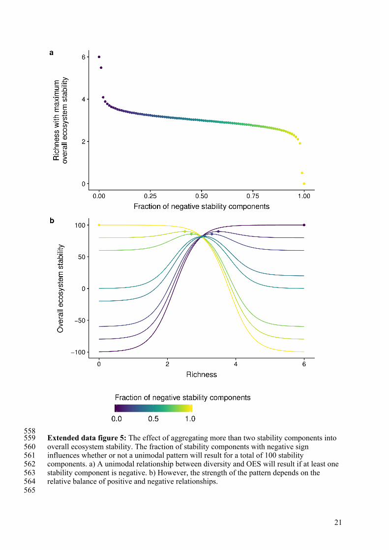
●
●
●
●
●
●
●
●
● ●●
●
●
●
●
●
●
●
●
●
●
●
●
●
●
●
● ●
●
●
●
●
●
●●
●
●
●●
●
●
●● ●
●
●
●
●
●
●
●
●
●
●
●
●
●
●●
●
●
●
●
●
●
●
●
●
●
●
●
●
●
●
● ●
●
●
●
●
●
●
●
●
●
●
●
●
●
●
●
●
●
●
●
●
●
●
●
●
●
●
●
●
●
●
●
●
●
●
●
●
●
●
●
● ●●
●
● ●
●
●
●
● ●
●
●
●
●
●
●
●
●
●
●
●
●
● ●
●
●
●●
●
●
●
●
●
● ●●
●
●
● ●
●
●
●
●
●● ●
●
●
●
●
●
●
●
●
●
●●●
●
●
●
●
● ●
●
●
●
●
●
●
●
●
●
●
●
●
●
●
●
●
●
●
●
●
●
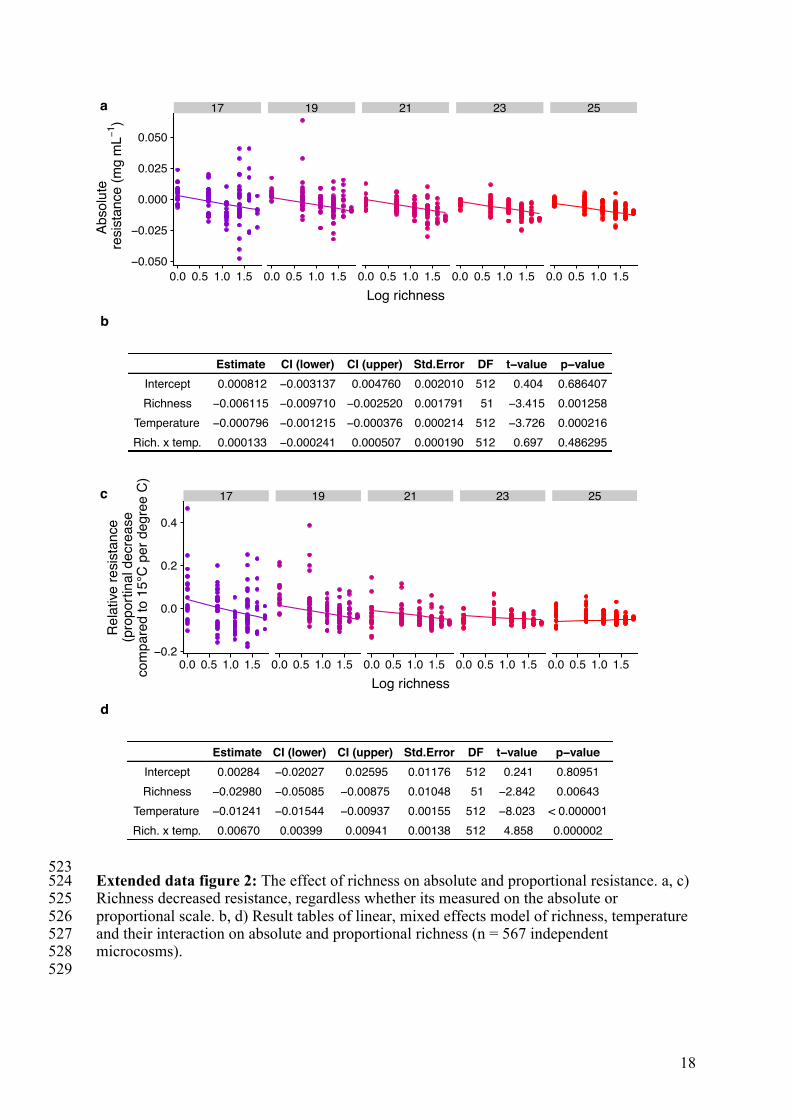
●
●●
●
●
●
●
●
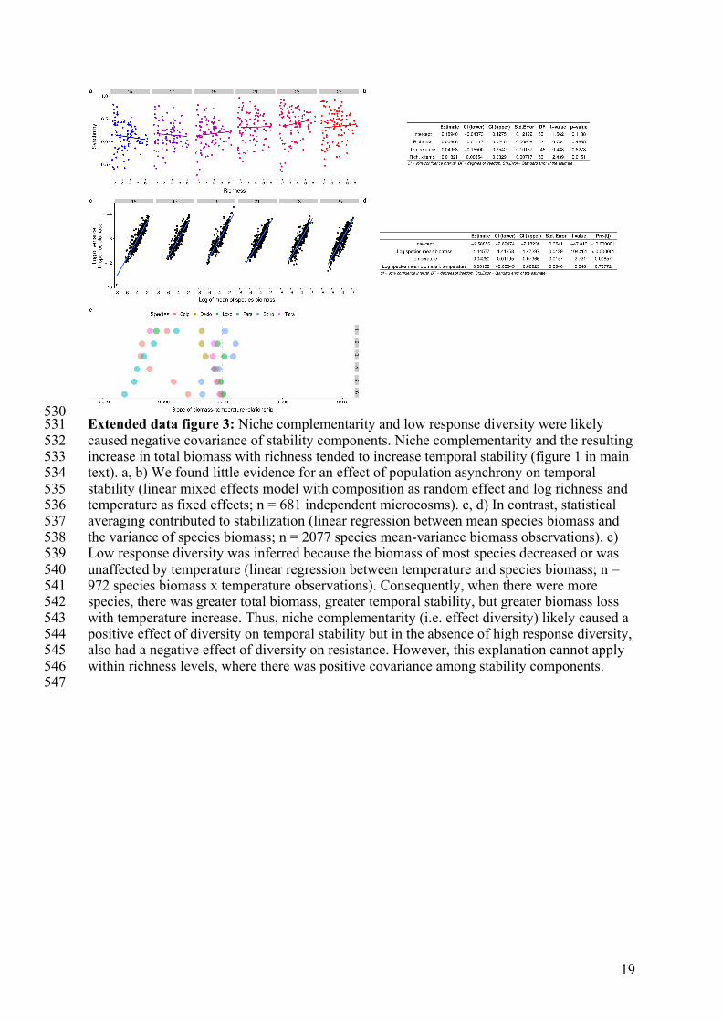
●
●
●
●
●
●●
●
●
●
●
●
●
●
●
●
●●
●
●
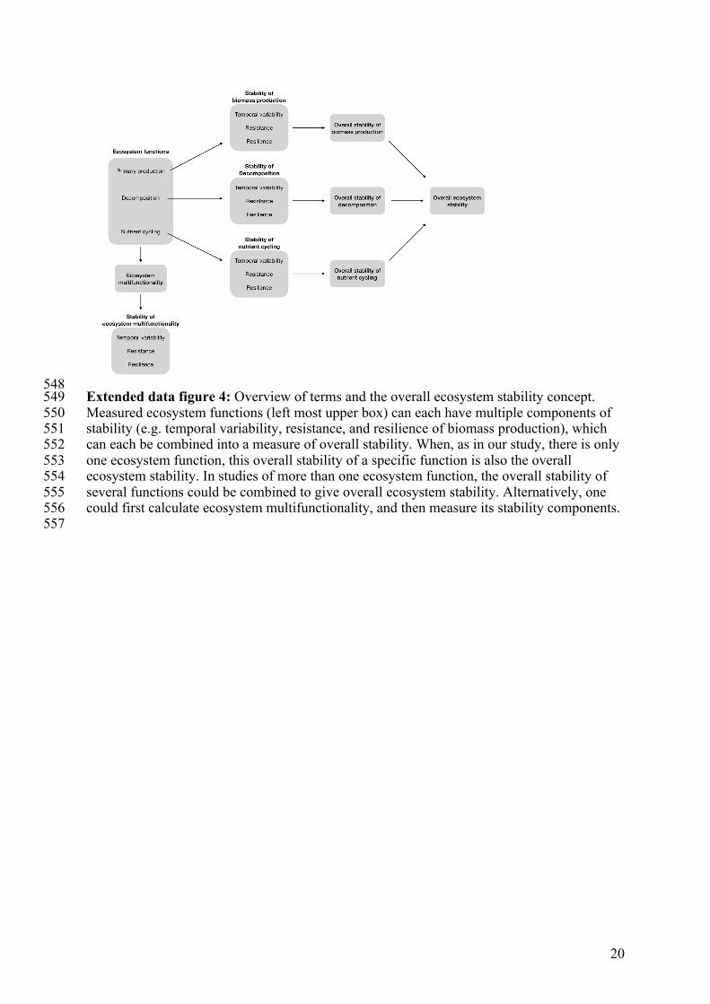
●
●
●
●
●
●
●
●
●
●
●
● ●
●
●●
●●
●
●
●
●
●
●
●
●
●
●
●
●
●●
● ●●
●
●
●
●
●
●
●
●
●
●●
●
●
●
●
●
●
●
●●
●
●
●
●
●
●
●
● ●
●
●
●
●●
●
●
●
● ●
●
●●●
●
●
●
●
●
●
●
●
●
●●●
●
●
●
●
●
●●
●
●
●
●
●
●
●
●
●
●
●
●
●
●
●●
●
●
●
●
●
●
●
●
●
●
●
●
●
●● ●
●●
●
●●
●● ●
●
●
●
●
●
●
●
● ●
●
●● ●
●
●
●
●
●
●
●
●
●
●
●
●
●
●
●
●
●
●
●
●
●
●
●
●
●
●
●
●
●
●
●
●
●
●
●
● ●
●
●
●
●
●
●
●
●
●
●●
●
●
●
●
1
2
3
4
5
1 2 3 4 5 6
Richness
Tem
pora
lst
abilit
y(m
ean/
STD
)
a1
●
●
●
●●
●
●
●● ●● ●●
●
●
●
●
●
●●
●●
●
●● ●●●●
●
●
●
●
●
●
●
● ●
●
●
●●
●
●
●
●
●●
●●
● ● ● ●●● ●
●
●
●●
●
● ●
●●●●
●●
●●
●● ●
● ●
●●●
●● ●●
●●
● ●●
●●
●
●●
●
●
●
●
●●
●
●●
●
●
●
●
●
●● ●● ●
●
●
●●
●
●●●●●
●
●●
●●
●
●●
● ●
●
●
●●
●
●
● ●●●
●
●
●
● ●●
●
●
●
●●
●
●
●●
●●● ●
●
●●
●
●
●
●
●
●
●
●
●
●
●● ●● ●
●●
●
●●●
●●
●●● ●
●
●
●●●
●● ●
●
●
●
●
●
●
●
●
●
●
●
● ●
●
●●
●●
●
●●●
●
●
●
●
●●
●●
●●
●
●
●
●
●
●
●● ●
●
●
●
●
●
● ●●
●●● ●
●●
●
●
●●
●● ●
●●
●
●
●●
●●
●●
●●
●
●
●
●●●
●●
●
●
●
●
●●
●
●●
●
● ●
●
●
●●
●●
●
●●
●
●●●
●
● ●●●
●
●● ●
●●● ●●
●
●●
●
●
●
●●● ●
●
●●
●
●
●●
●●
● ●
●
●
●
●
●
●●
●
● ●
●
●●
●
●●
●●●
●
●●
●
●
●
● ●●
●●
●●
●
●
●
●●
●●
●
●
●
●
●
●
●●●
● ●
●
●
●
●●
●
● ●
●●●
●
●●
●●●
●●●
●
●●
●
●
●
●●●
●
●
●
●
●
●
●
●●
●
●
●
●
●●
●●
● ● ●
●
●
●
●
●●●●
●
● ●
●●
●
●
●
●
●●
●●
●●
●
●●
●● ●●
●
●●
●
●
● ●●
●● ●
●●
●
●
●
●
●
●●
●
●●
●
●
●
● ●●●
●
●
●
●
●●
●
●
●
●
●
●
● ●
●
● ●
●
●● ●
●
●
●
●
●
● ●
●●
●
●
●
●
●
●
●● ●●
●
●
●
●
● ●
●●●
● ●
●
●●
−0.050
−0.025
0.000
0.025
0.050
1 2 3 4 5 6
Richness
Res
ista
nce
(Dm
illigr
am/m
L)
a2
−0.0050
−0.0025
0.0000
0.0025
5 10 15
Tem
pera
ture
mai
n ef
fect
c1
0.000
0.025
0.050
0.075
0.100
5 10 15
Log(
richn
ess)
mai
n ef
fect
c2
−0.010
−0.005
0.000
0.005
5 10 15
Day
Inte
ract
ion
c3
0.05
0.10
0.15
0.20
0 10 20 30
DayBi
omas
s (m
illigr
am/m
L)
richness 1 2 3 4 5 6b
x xxxx x
−0.050
−0.025
0.000
0.025
0.050
1 2 3 4 5
Temporal stability
Res
ista
nce
d
15
492 Figure 2: Positive, negative and neutral relationships among resistance, resilience and temporal 493 variability in empirical studies with diversity manipulation. 30 bivariate relationships were reported by 17 494 independent studies (in addition to this study). Detailed information about individual studies (e.g. code VR-09) 495 is provided in extended data table 3 & 4. Beige regions indicate no covariation. Relative positions within 496 regions are arbitrary and do not indicate relative strengths of relationships. Different colours indicate the effect 497 of diversity on absolute (red) or relative resistance (blue), whereas temporal stability and resilience are shown in 498 black. 499 500
Ba−16
Gr−00−1
Gr−00−2
Hu−04
Is−15
PS−02 PS−02
TD−94
Ti−96
Vo−12
Vo−12
VR−10VR−10
Wa−00
Wa−17
We−07Wr−15
Z1−06 *Z2−06
(+/+)0(−/+)
(+/−)0(−/−)
0 0
Diversity − resistance
Dive
rsity
− re
silie
nce
Ca−05
Ca−05
Is−15
Ti−96
Wa−17
Z1−06 *
(+/+)0(−/+)
(+/−)0(−/−)
0 0
this study
Diversity − temporal variability
Dive
rsity
− re
sist
ance
Is−15
Ti−96
Wa−17
Z1−06 *
(+/+)0(−/+)
(+/−)0(−/−)
0 0
Diversity − temporal variability
Dive
rsity
− re
silie
nce
16
501 Figure 3: Hump- and U-shaped diversity-stability relationships. The intercept of the generalised logistic to 502 convert measured stability components into a common currency varies with parameter Q (a). The non-503 aggregated (n = 567 independent microcosms) or aggregated (n = 6 richness levels) data exhibits hump- to flat- 504 to U-shaped diversity-stability relationships as Q varies. Lines show the fit of a quadratic model and the 95% 505 confidence interval (bands). (b). The variation from hump-shaped to U-shaped relationship depends smoothly 506 on Q, i.e. the position of the threshold (quantified by the quadratic term of a regression with mean (dot) and 507 95% confidence intervals (bars)) (c). 508 509 510
0.01 1 100
function−2 −1 0 1 2 −2 −1 0 1 2 −2 −1 0 1 2
−1.0
−0.5
0.0
0.5
1.0
Stability component
Con
verte
d st
abilit
y va
lue
a
Q: 0.01 Q: 1 Q: 100
level: microcosm
level: richness
2 4 6 2 4 6 2 4 6
−2
−1
0
1
2
−2
−1
0
1
2
3
Richness
Ove
rall
ecos
yste
m s
tabi
lity
b
−2
0
2
4
−2 −1 0 1 2
log10(Q)
Qua
drat
ic te
rm(+−
2 st
anda
rd e
rrors
)
level
microcosm
richness
c
17
Extended data figures: 511 512
513 Extended data figure 1: Richness increased temporal stability across temperatures. a) The 514 stabilizing effect of richness was present across all temperatures, although temperature has a 515 negative effect on mean stability. b) Result table for linear, mixed effects model of log 516 richness, temperature and their interaction on temporal stability supporting the stabilizing 517 effects of richness and the negative effect of temperature on temporal stability (n = 681 518 independent microcosms). c) Result table for the same analysis as b) but without the 519 monocultures. Results are qualitatively the same, indicating that the relationship between 520 richness and temporal stability is not only driven by the monocultures (n = 580 independent 521 microcosms). 522
18
523 Extended data figure 2: The effect of richness on absolute and proportional resistance. a, c) 524 Richness decreased resistance, regardless whether its measured on the absolute or 525 proportional scale. b, d) Result tables of linear, mixed effects model of richness, temperature 526 and their interaction on absolute and proportional richness (n = 567 independent 527 microcosms). 528 529
17 19 21 23 25
0.0 0.5 1.0 1.5 0.0 0.5 1.0 1.5 0.0 0.5 1.0 1.5 0.0 0.5 1.0 1.5 0.0 0.5 1.0 1.5−0.050
−0.025
0.000
0.025
0.050
Log richness
Abso
lute
res
ista
nce
(mg
mL−
1 )a
Intercept
Estimate
Richness
CI (lower)
Temperature
CI (upper)
Rich. x temp.
Std.Error 0.000812
DF
−0.006115
t−value
−0.000796
p−value
0.000133
−0.003137−0.009710−0.001215−0.000241
0.004760−0.002520−0.000376 0.000507
0.0020100.0017910.0002140.000190
512 51512512
0.404−3.415−3.726 0.697
0.6864070.0012580.0002160.486295
b
17 19 21 23 25
0.0 0.5 1.0 1.5 0.0 0.5 1.0 1.5 0.0 0.5 1.0 1.5 0.0 0.5 1.0 1.5 0.0 0.5 1.0 1.5−0.2
0.0
0.2
0.4
Log richness
Rel
ative
resi
stan
ce(p
ropo
rtina
l dec
reas
eco
mpa
red
to 1
5°C
per
deg
ree
C)
c
Intercept
Estimate
Richness
CI (lower)
Temperature
CI (upper)
Rich. x temp.
Std.Error 0.00284
DF
−0.02980
t−value
−0.01241
p−value
0.00670
−0.02027−0.05085−0.01544 0.00399
0.02595−0.00875−0.00937 0.00941
0.011760.010480.001550.00138
512 51512512
0.241−2.842−8.023 4.858
0.809510.00643
< 0.0000010.000002
d
19
530 Extended data figure 3: Niche complementarity and low response diversity were likely 531 caused negative covariance of stability components. Niche complementarity and the resulting 532 increase in total biomass with richness tended to increase temporal stability (figure 1 in main 533 text). a, b) We found little evidence for an effect of population asynchrony on temporal 534 stability (linear mixed effects model with composition as random effect and log richness and 535 temperature as fixed effects; n = 681 independent microcosms). c, d) In contrast, statistical 536 averaging contributed to stabilization (linear regression between mean species biomass and 537 the variance of species biomass; n = 2077 species mean-variance biomass observations). e) 538 Low response diversity was inferred because the biomass of most species decreased or was 539 unaffected by temperature (linear regression between temperature and species biomass; n = 540 972 species biomass x temperature observations). Consequently, when there were more 541 species, there was greater total biomass, greater temporal stability, but greater biomass loss 542 with temperature increase. Thus, niche complementarity (i.e. effect diversity) likely caused a 543 positive effect of diversity on temporal stability but in the absence of high response diversity, 544 also had a negative effect of diversity on resistance. However, this explanation cannot apply 545 within richness levels, where there was positive covariance among stability components. 546 547
20
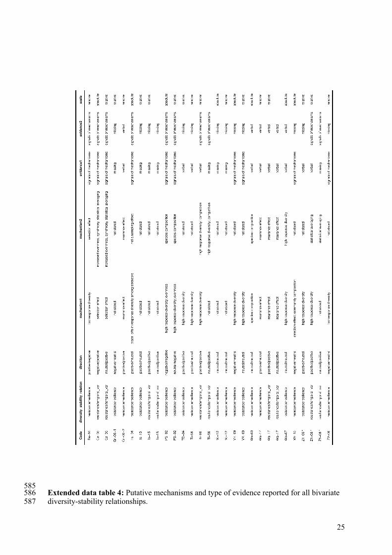
548 Extended data figure 4: Overview of terms and the overall ecosystem stability concept. 549 Measured ecosystem functions (left most upper box) can each have multiple components of 550 stability (e.g. temporal variability, resistance, and resilience of biomass production), which 551 can each be combined into a measure of overall stability. When, as in our study, there is only 552 one ecosystem function, this overall stability of a specific function is also the overall 553 ecosystem stability. In studies of more than one ecosystem function, the overall stability of 554 several functions could be combined to give overall ecosystem stability. Alternatively, one 555 could first calculate ecosystem multifunctionality, and then measure its stability components. 556 557
21
558 Extended data figure 5: The effect of aggregating more than two stability components into 559 overall ecosystem stability. The fraction of stability components with negative sign 560 influences whether or not a unimodal pattern will result for a total of 100 stability 561 components. a) A unimodal relationship between diversity and OES will result if at least one 562 stability component is negative. b) However, the strength of the pattern depends on the 563 relative balance of positive and negative relationships. 564 565
22
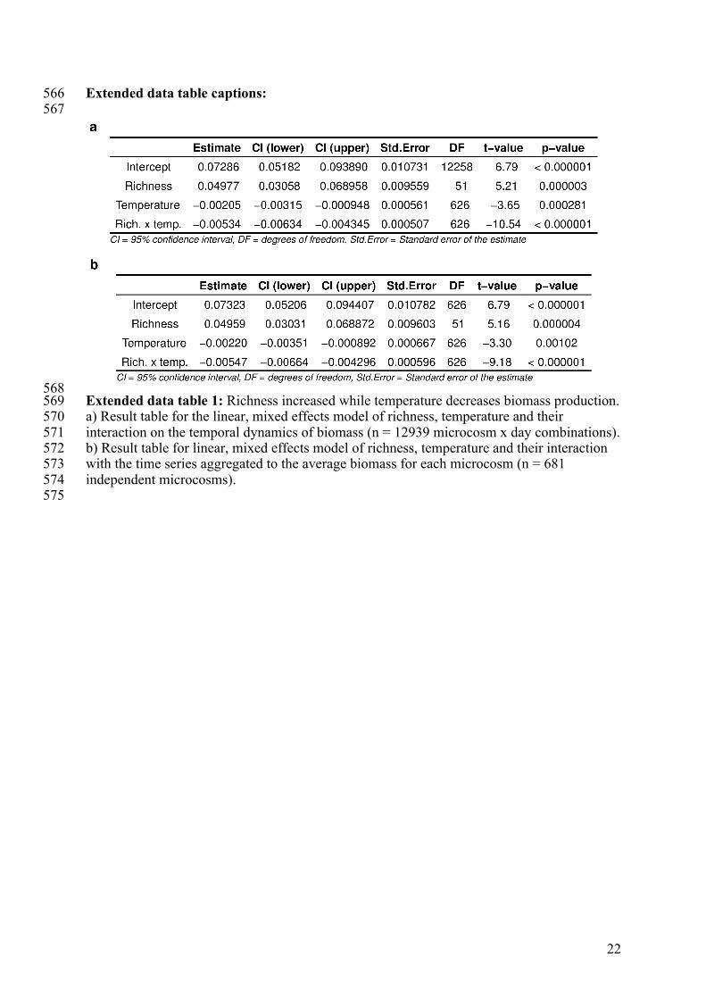
Extended data table captions: 566 567
568 Extended data table 1: Richness increased while temperature decreases biomass production. 569 a) Result table for the linear, mixed effects model of richness, temperature and their 570 interaction on the temporal dynamics of biomass (n = 12939 microcosm x day combinations). 571 b) Result table for linear, mixed effects model of richness, temperature and their interaction 572 with the time series aggregated to the average biomass for each microcosm (n = 681 573 independent microcosms). 574 575
23
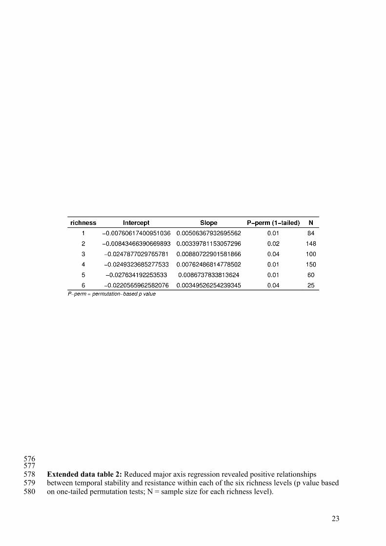
576 577 Extended data table 2: Reduced major axis regression revealed positive relationships 578 between temporal stability and resistance within each of the six richness levels (p value based 579 on one-tailed permutation tests; N = sample size for each richness level). 580
24
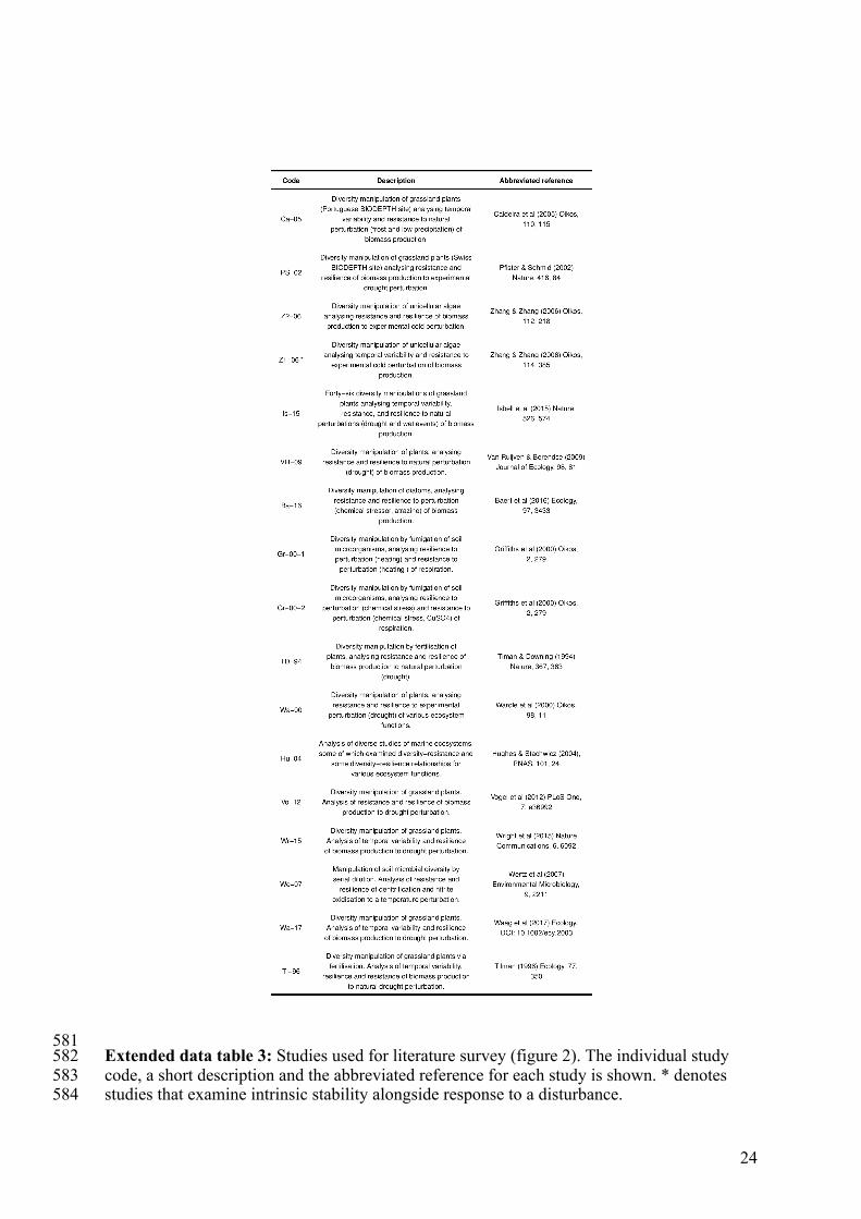
581 Extended data table 3: Studies used for literature survey (figure 2). The individual study 582 code, a short description and the abbreviated reference for each study is shown. * denotes 583 studies that examine intrinsic stability alongside response to a disturbance. 584
25
585 Extended data table 4: Putative mechanisms and type of evidence reported for all bivariate 586 diversity-stability relationships. 587