BIQUOTIENTS WITH ALMOST POSITIVE CURVATURE

Martin Kerin

A Dissertation

in

Mathematics

Presented to the Faculties of the University of Pennsylvania in PartialFulfillment of the Requirements for the Degree of Doctor of Philosophy

2008

Wolfgang ZillerSupervisor of Dissertation

Tony PantevGraduate Group Chairperson

Acknowledgments

I’ve never been one to do things by halves. This is going to be long.

Words will never be able to express the full extent of my gratitude to my advisor,

Wolfgang Ziller. Without his guidance, inspiration, boundless enthusiasm, good

nature, tolerance for ridiculous questions, encouragement, wisdom and seemingly

limitless knowledge, none of this could have been accomplished. It will forever bring

a smile to my face to imagine him beside me at the board excitedly discussing some

new proof or the consequences of some result, not to mention his complete lack of

understanding of how soccer could possibly be more important than mathematics.

Perhaps the highest compliment I can pay him is that I cannot even begin to imagine

having studied under the direction of anyone else. I’d like to think that he enjoyed

having me as his student half as much as I enjoyed being in that position. I’m only

contrary with the people I like, and he got double doses. I know he’s going to miss

my stubbornness, even though he may never acknowledge that fact.

A special word of thanks is reserved for my friend and former M.Sc. advisor,

David Wraith. Many times I returned to his office in Maynooth in a dejected state,

ii

wondering what I was doing with my life. His understanding, encouragement, belief

and friendship gave me renewed hope and the determination to continue. He was

the catalyst for all of this and the person who taught me to aim high.

My parents have always trusted me to make good decisions and have never tried

to prevent me from pursuing this ridiculous hobby, even if they are completely

bewildered as to why anyone would wish to do such a thing. Their strength and

wisdom is an inspiration to me, and frequent sullen phone calls are poor reward for

their support. They are my heroes and my greatest teachers, even if I don’t say it

aloud.

I must not forget Chris Croke, who stood in as my surrogate daddy while Wolf-

gang was off sunning himself in Rio. He did a fine job and is indirectly responsible

for the subject of this work.

The worst kept secret in the department, the so-called “Secret Seminar”, was

both enjoyable and beneficial. The participants made it what it was and so, Kris,

Corey, John, Chenxu, Ricardo, and Jason, you have my thanks.

The completion of this dissertation reminds me of how it began, and the price I

had to pay. Maria’s strength in letting me go is humbling. I am truly sorry for the

pain I caused her. We will never know what could have been, but our friendship

will last eternal.

Thanks must go to the Dancers, who tolerate my sleeping on their couch for

weeks at a time and never shy away from taking me down a peg or two, to Ciaran

iii

and Adrian for being more than friends, to Tadhg, Melody, Al, and all my other

Irish friends. Trips home wouldn’t have been the same without you guys, and played

their own vital role in this whole nonsense.

Pilar, David, Lee, Armin, Shea, Wil, Chris, Jen, Mike, Andrew, Jimmy, Joe,

Enka, to name but a few. Nerds, but good nerds.

Dan Jane and I have shared many adventures between Berkeley and Brazil.

Without his influence I would not have enjoyed my second trip to Brazil quite as

much as I did, nor found the balance between mathematics and surfing. I hope we

have many adventures ahead of us.

Mike Suarez, Leslie and Amy were friends in Philly as rare and exceptional as

any of those I have in Ireland. The days are lonelier without having them around,

even if we never got to see as much of each other as we may have wanted when we

had the opportunity.

West Philly F.C. kept me sane, perhaps the most difficult job of all, and I’ll be

sorry to leave them.

Finally I would like to express my thanks to the four wonderful ladies who make

the department function, Janet, Monica, Paula and Robin. These four ladies are

always there whenever anyone needs anything and I’m not sure that they are aware

of how much they are appreciated. My days would not have been the same without

their smiles, advice, help, tolerance and consideration. I will miss our chats, slacking

off in their offices, and all the birthday cakes.

iv

ABSTRACT

BIQUOTIENTS WITH ALMOST POSITIVE CURVATURE

Martin Kerin

Wolfgang Ziller, Advisor

When does a manifold admit a metric with positive sectional curvature? This

is one of the most fundamental and difficult problems in differential geometry. One

attempt at understanding this problem is to begin with a non-negatively curved

manifold and examine how large is the set of points with positive curvature. More

precisely, given a manifold, does it admit a non-negatively curved metric for which

there is an open set of points with positive curvature (quasi-positive curvature), or

an open dense set of such points (almost positive curvature)? We construct new

examples of biquotients which admit such metrics.

v

Contents

1 Introduction 1

2 Biquotient actions and metrics 13

2.1 Biquotients . . . . . . . . . . . . . . . . . . . . . . . . . . . . . . . 13

2.2 Submersions and metric deformations . . . . . . . . . . . . . . . . . 15

3 Eschenburg Spaces 22

3.1 Eschenburg’s results . . . . . . . . . . . . . . . . . . . . . . . . . . 22

3.2 New results . . . . . . . . . . . . . . . . . . . . . . . . . . . . . . . 25

3.3 Lens spaces and closed geodesics . . . . . . . . . . . . . . . . . . . . 32

4 Bazaikin Spaces 38

4.1 Positive curvature . . . . . . . . . . . . . . . . . . . . . . . . . . . . 38

4.2 Almost and quasi-positive curvature . . . . . . . . . . . . . . . . . . 47

5 Quotients of S7 × S7 51

5.1 The Cayley numbers, G2 and its Lie algebra . . . . . . . . . . . . . 51

vi

5.2 Free isometric actions on SO(8) . . . . . . . . . . . . . . . . . . . . 54

5.3 Quasi-positive curvature . . . . . . . . . . . . . . . . . . . . . . . . 61

5.4 Topology . . . . . . . . . . . . . . . . . . . . . . . . . . . . . . . . . 66

6 Torus quotients of S3 × S3 97

6.1 Free and almost free T 2 actions on S3 × S3 . . . . . . . . . . . . . . 97

6.2 Curvature on (S3 × S3)//T 2 . . . . . . . . . . . . . . . . . . . . . . 106

vii

List of Tables

3.1 Conditions for positive curvature on Lij . . . . . . . . . . . . . . . . 36

3.2 Conditions for positive curvature on Cσ . . . . . . . . . . . . . . . . 37

5.1 Multiplication table for Ca . . . . . . . . . . . . . . . . . . . . . . . 52

6.1 Isotropy groups of the T 2 actions Uc, Uc, Ua,b and Ua,b . . . . . . . . 104

6.2 Some special cases of the action of Uc, c even . . . . . . . . . . . . . 104

6.3 Some special cases of the action of Uc, c odd . . . . . . . . . . . . . 104

6.4 Some special cases of the action of Ua,b, a + b even . . . . . . . . . . 105

6.5 Some special cases of the action of Ua,b, a + b odd . . . . . . . . . . 105

viii

Chapter 1

Introduction

When does a manifold admit a metric with positive sectional curvature? This is a

fundamental and difficult problem in differential geometry. There are many exam-

ples of manifolds with non-negative curvature. For example, all homogeneous spaces

G/H and all biquotients G//U inherit non-negative curvature from the bi-invariant

metric on G. It was also shown in [GZ1] that all cohomogeneity-one manifolds,

namely manifolds admitting an isometric group action with one-dimensional orbit

space, with singular orbits of codimension ≤ 2 admit metrics with non-negative

curvature.

On the other hand, the known examples with positive curvature are very sparse.

Other than the rank-one symmetric spaces there are isolated examples in dimensions

6, 7, 12, 13 and 24 due to Wallach [Wa] and Berger [Ber2], and two infinite families,

one in dimension 7 (Eschenburg spaces; see [AW], [E1], [E2]) and the other in

1

dimension 13 (Bazaikin spaces; see [Ba1]).

In the simply connected case there are no known obstructions to admitting

positive curvature that are not already obstructions to admitting a metric of non-

negative curvature. Some of the standard theorems relating topology and positive

curvature are:

Bonnet-Myers Let Mn be a complete Riemannian manifold and suppose that the

Ricci curvature satisfies Ric ≥ δ > 0. Then M is compact and π1(M) is finite.

Synge Let Mn be a compact manifold with positive sectional curvature, sec > 0.

(i) If M is orientable and n is even, then M is simply connected;

(ii) If n is odd, then M is orientable.

Sphere Theorem Let Mn be a compact, simply connected, Riemannian manifold.

(i) If 1 < sec ≤ 4 then Mn is diffeomorphic to Sn;

(ii) If 1 ≤ sec ≤ 4 then Mn is either diffeomorphic to Sn or isometric to a

CROSS.

The Sphere Theorem was established up to homeomorphism by Berger [Ber1] and

Klingenberg [K], and up to diffeomorphism by Brendle and Schoen [BS1], [BS2].

In fact, Brendle and Schoen proved more general rigidity results which imply the

Sphere Theorem as a special case. Soon after the announcement of the proof by

Brendle and Schoen, Ni and Wolfson [NW] announced an alternate proof in the

special case of the differential Sphere Theorem.

2

We are interested in the study of manifolds which lie “between” those with

non-negative and those with positive curvature.

Definition. A Riemannian manifold (M, 〈 , 〉) has quasi-positive curvature (resp.

almost positive curvature) if (M, 〈 , 〉) has non-negative sectional curvature and

there is a point (resp. an open dense set of points) at which all 2-planes have

positive sectional curvature.

It should be noted that in the definition of quasi-positive curvature we could

replace “point” with “an open set of points”.

One of the major motivations for studying manifolds with quasi-positive curva-

ture is the well-known Deformation Conjecture which we rewrite in our language.

Conjecture. Suppose (M, 〈 , 〉) is a complete Riemannian manifold with quasi-

positive curvature. Then M admits a metric with positive curvature.

There is some evidence in support of this conjecture. Aubin [Au] and Ehrlich

[Eh] proved the analogous statements for scalar and Ricci curvature. Perelman’s

proof of the soul conjecture [Pe] shows that a non-compact manifold with quasi-

positive curvature is diffeomorphic to Rn and hence admits a metric with positive

curvature. Moreover, Hamilton [Ha] has shown that the Deformation Conjecture is

true in dimension three.

Petersen and Wilhelm [PW] provided the first examples of manifolds with almost

positive curvature when they showed that the unit tangent bundle of S4 and a real

cohomology CP 3 admit such metrics.

3

Most of the known examples of manifolds with almost positive curvature appear

in the work of Wilking [Wi]. In particular he proves that

Theorem (Wilking). Each of the following compact manifolds admits almost pos-

itive curvature.

(i) The projective tangent bundles PRTRP n, PCTCP n, and PHTHP n of RP n,

CP n and HP n respectively.

(ii) The homogeneous space M4n−1k,` = U(n + 1)/Hk,`, with k, ` ∈ Z, k` < 0, and

n ≥ 2, where

Hk,` = diag(zk, z`, A) | z ∈ S1, A ∈ U(n− 1).

Since the universal cover of PRTRP n is T 1Sn, the unit tangent bundle of Sn,

it is clear that T 1Sn also admits a metric with almost positive curvature. We also

note that Wallach [Wa] has shown that the flag manifolds PCTCP 2 and PHTHP 2

admit homogeneous metrics with positive curvature.

The homogeneous spaces described by M4n−1k,` should be thought of as generali-

sations of the 7-dimensional positively curved Aloff-Wallach spaces, W 7k,`. However

it is clear that the metric on M4n−1k,` cannot be homogeneous, since otherwise we

could left-translate a zero-curvature plane to every point of M4n−1k,` . Furthermore,

an examination of the Gysin sequence for the fibration S1 −→ M4n−1k,` −→ PCTCP n

shows that there are infinitely many homotopy types of simply connected manifolds

of a fixed dimension 4n − 1 which admit almost positive curvature. Recall that

4

the Aloff-Wallach spaces are homogeneous spaces SU(3)/S1k,`, where S1

k,` ⊂ SU(3)

via z 7−→ diag(zk, z`, zk+`). Of course W 7k,` may be rewritten in the form M4n−1

k,`

with n = 2 as in Wilking’s theorem. In [AW] the authors show that W 7k,` admits

positive curvature if and only if k`(k + `) 6= 0. There is thus a unique Aloff-Wallach

space, namely W 7−1,1, which is not known to admit positive curvature. Since left-

translation is an isometry, it is clear that W 7−1,1 must have a zero-curvature plane at

every point with respect to the homogeneous metric. Therefore we see that Wilk-

ing’s result deforms the homogeneous metric on W 7−1,1 to a non-homogeneous metric

with almost positive curvature. The integral cohomology ring of W 7−1,1 is the same

as that of S2× S7 and it is an open problem to decide whether these manifolds are

homotopy equivalent.

Notice that Wilking shows there are odd-dimensional, non-orientable manifolds,

for example RP 3 × RP 2 and RP 7 × RP 6, which admit almost positive curvature.

By Synge’s Theorem such manifolds cannot admit positive curvature. Thus these

manifolds are counter-examples to the Deformation Conjecture. However, all of

these counter-examples have non-trivial fundamental group. Therefore it is still

possible that the Deformation Conjecture holds for simply connected manifolds with

quasi-positive curvature. Moreover, in [PW] the authors suggest that consideration

should be given to the following modification of the Deformation Conjecture:

Question. Does a Riemannian manifold with quasi-positive curvature admit a met-

ric with almost positive curvature?

5

From Wilking’s counter-examples to the Deformation Conjecture we see that the

class of manifolds admitting almost positive curvature is strictly larger than the class

of manifolds admitting positive curvature. Moreover, the class of manifolds having

quasi-positive curvature is strictly contained in the class of non-negatively curved

manifolds, as a necessary condition for admitting quasi-positive curvature is the

possession of a finite fundamental group. This follows in the non-compact case from

Perelman’s proof of the soul conjecture [Pe], and in the compact case from Bonnet-

Myers together with the results of Aubin [Au] and Ehrlich [Eh] on deformations of

metrics with non-negative Ricci curvature and positive Ricci curvature at a point.

From the question above we see that it is unknown whether the class of almost

positively curved manifolds is strictly contained in the class of those with quasi-

positive curvature.

There is an even more profound reason for investigating the validity of the

Deformation Conjecture for simply connected manifolds. The fact that RP 3×RP 2

and RP 7×RP 6 admit metrics with almost positive curvature implies that S3× S2

and S7 × S6 admit such metrics. If it were possible to deform these metrics to

have positive curvature then we would have counter-examples to the celebrated

Hopf Conjecture, which asserts that a product of spheres cannot admit positive

curvature.

The first example of a manifold with quasi-positive curvature was given in [GM,

’74]. Here it was shown that the Gromoll-Meyer exotic 7-sphere Σ7 = Sp(2)//Sp(1)

6

inherits quasi-positive curvature from the bi-invariant metric on Sp(2). In [W, ’01]

Wilhelm showed that the bi-invariant metric on Sp(2) may be deformed in such a

way as to induce almost positive curvature on Σ7. The deformed metric on Sp(2)

is no longer left-invariant. In [EK, ’07] it is shown that there exits a left-invariant

metric on Sp(2) which induces almost positive curvature on Σ7. The set of points

with zero-curvature planes is given by a finite union of subvarieties of codimension

≥ 1 and can be explicitly determined. If one could further deform the metric on Σ7

to have positive curvature, then it would be the first example of an exotic sphere

admitting a metric of this kind.

The only other previously known examples of manifolds with almost positive

or quasi-positive curvature are given in [PW, ’99], [Wi, ’01] and [Ta1, ’03]. In

particular Tapp shows:

Theorem (Tapp). The following manifolds admit metrics with quasi-positive cur-

vature:

(i) The unit tangent bundles T 1CP n, T 1HP n and T 1CaP2;

(ii) The homogeneous space M4n−1k,` = U(n+1)/Hk,`, with k, ` ∈ Z, (k, `) 6= (0, 0),

and n ≥ 2, where

Hk,` = diag(zk, z`, A) | z ∈ S1, A ∈ U(n− 1).

Notice that Tapp proves that those generalised Aloff-Wallach spaces M4n−1k,` for

which k` ≥ 0 admit quasi-positive curvature. These are exactly the M4n−1k,` not

7

included in Wilking’s examples of almost positively curved manifolds.

We recall briefly that the Eschenburg spaces are defined by E7p,q = SU(3)//S1

p,q

where p = (p1, p2, p3), q = (q1, q2, q3) ∈ Z3,∑

pi =∑

qi, and S1p,q acts on SU(3) via

z ? A = diag(zp1 , zp2 , zp3)A diag(zq1 , zq2 , zq3), z ∈ S1, A ∈ SU(3).

Similarly the Bazaikin spaces are defined by B13q1,...,q5

= SU(5)//(Sp(2) · S1q1,...,q5

),

where Sp(2) · S1q1,...,q5

= (Sp(2)× S1q1,...,q5

)/Z2 acts on SU(5) via

[A, z] ? B = diag(zq1 , . . . , zq5)B diag(A, zq),

z ∈ S1, A ∈ Sp(2) ⊂ SU(4), B ∈ SU(5), and q =∑

qi. We will discuss the

Eschenburg and Bazaikin spaces in much more detail in subsequent chapters.

We are now in a position to state our main result in which we describe some

new examples of manifolds admitting almost or quasi-positive curvature.

Theorem A.

(i) All Eschenburg spaces E7p,q = SU(3)//S1

p,q admit metrics with quasi-positive

curvature.

(ii) The Eschenburg space E7p,q, p = (1, 1, 0), q = (0, 0, 2), admits almost positive

curvature.

(iii) All Bazaikin spaces B13q1,...,q5

= SU(5)//(Sp(2) · S1q1,...,q5

) such that four of the

qj share the same sign admit quasi-positive curvature.

(iv) The Bazaikin space B13−1,1,1,1,1 admits almost positive curvature.

8

(v) There is a free circle action on S7×S7 such that M13 = S1\(S7×S7) admits a

metric with quasi-positive curvature. Furthermore, M13 is not homeomorphic

to CP 3 × S7.

(vi) There is a free S3-action on S7 × S7 such that N11 = S3\(S7 × S7) admits a

metric with quasi-positive curvature. Furthermore, N11 is not homeomorphic

to S4 × S7.

The topology of Eschenburg spaces has been studied extensively (see, for ex-

ample, [E2], [CEZ], [K1], [K2], [Sh2]). In particular the cohomology groups of

the Eschenburg spaces are H0 = H2 = H5 = H7 = Z and H4 = Z|s|, where

s := p1p2 + p1p3 + p2p3− q1q2− q1q3− q2q3. Moreover s is always odd (see [K1], Re-

mark 1.4). There is a special subfamily of Eschenburg spaces with p = (1, 1, n), q =

(0, 0, n + 2) ([Sh2], [GSZ]) which we denote by E7n. We note that E7

n and E7−(n+1)

describe the same manifold, and E7n has positive curvature if n ≥ 1 ([E1]). Since

H4(E7n) = Z2n+1, n ≥ 0, it is clear that every cyclic group of odd order is achieved,

and moreover that there are infinitely many positively curved Eschenburg spaces

which are distinct even up to homotopy equivalence. We note that, as for the Aloff-

Wallach space W 7−1,1, the integral cohomology ring of E7

0 agrees with that of S2×S5

and it is unknown whether these manifolds are homotopy equivalent. On the other

hand, in [CEZ] it is shown that there are only finitely many positively curved Es-

chenburg spaces for a given cohomology ring. This should be viewed in the context

of the Klingenberg-Sakai conjecture. It states that there are only finitely many pos-

9

itively curved manifolds in a given homotopy type, and the result in [CEZ] raises

the question of whether the conjecture is true even for cohomology. In the present

context, it is natural to ask the following question.

Question. Are there infinitely many pairwise non-homotopy equivalent Eschenburg

spaces which share the same cohomology ring?

In the event of a positive answer to this question, only finitely many of these

Eschenburg spaces can admit positive curvature by our previous remark. Theorem

A(i) would provide the first examples of infinite families of simply connected, non-

homotopy equivalent manifolds with quasi-positive curvature which share the same

cohomology.

Notice that the resolution of this question again highlights the importance of the

Deformation Conjecture for simply connected manifolds with quasi-positive curva-

ture. If the Deformation Conjecture is true in this case, then the cohomology

Klingenberg-Sakai Conjecture is false. Equivalently, if the cohomology Klingenberg-

Sakai conjecture is true, then the Deformation Conjecture must clearly be false for

simply connected manifolds.

It follows from the results in [FZ1] that, although the almost positively curved

Bazaikin space B13−1,1,1,1,1 has the same integral cohomology ring as CP 2 × S9, con-

sideration of the respective Pontrjagin classes shows that these manifolds are not

even homotopy equivalent. Using results of Taimanov [T], one easily notices that

B13−1,1,1,1,1 contains both the exceptional Aloff-Wallach space W 7

−1,1 and the Eschen-

10

burg space E70 as totally geodesic submanifolds (Proposition 4.2.3). Theorem A(ii)

shows that E70 also admits almost positive curvature, whereas W 7

−1,1 has a zero-

curvature plane at every point ([AW]). As we discussed earlier, Wilking [Wi] has

shown that one can deform the metric on W 7−1,1 such that it admits almost positive

curvature.

If we now relax the constraint that U acts freely on G by allowing U to act

almost freely (i.e. all isotropy groups are finite), then we can find the following

orbifold examples:

Theorem B.

(i) All of the Eschenburg orbifolds E7p,q = SU(3)//S1

p,q with p = (p1, p2, p3), q =

(q1, q2, q3) ∈ Z3 satisfying

q1 < q2 = p1 < p2 ≤ p3 < q3 (†)

admit almost positive curvature.

(ii) There are infinitely many orbifolds of the form (S3×S3)//T 2 admitting almost

positive curvature.

Remark (a). There are no free S1p,q-actions on SU(3) satisfying condition (†). More-

over, (†) is essential to the proof of almost positive curvature, i.e. we cannot use a

similar proof to get almost positive curvature for free actions.

Remark (b). It is interesting to note that for the T 2-actions on S3 × S3 which we

consider the proof of almost positive curvature on (S3×S3)//T 2 breaks down exactly

11

when the action is required to be free, namely for the quotient manifolds S2 × S2

and CP 2# CP2.

Remark (c). Among the orbifolds (S3 × S3)//T 2, there are examples with one sin-

gular point with Z3-isotropy, and examples with two singular points, each with

Z2-isotropy. These examples are described in Tables 6.2, 6.3, 6.4 and 6.5.

12

Chapter 2

Biquotient actions and metrics

In his Habilitation, [E1, ’84], Eschenburg studied biquotients in great detail. In

particular he provided a classification of maximal rank torus actions on simple

Lie groups. The following sections borrow heavily from the material in [E1] and

establish the basic language, notation and results which will be used throughout

the subsequent chapters.

2.1 Biquotients

Let G be a compact Lie group, U ⊂ G×G a closed subgroup, and let U act on G

via

(u1, u2) ? g = u1gu−12 , g ∈ G, (u1, u2) ∈ U.

The action is free if and only if, for all non-trivial (u1, u2) ∈ U , u1 is never conjugate

in G to u2. The resulting manifold is called a biquotient.

13

Recall that every element of a compact Lie group is conjugate to an element of

‘the’ maximal torus. Thus in order to check that the action of U ⊂ G×G on G is

free it is enough to show that t1 and t2 are never conjugate in G, where (t1, t2) is a

non-trivial element of U ∩ (T ×T ), T a maximal torus of G. Therefore checking for

freeness is enormously simplified and often reduces to comparing the eigenvalues of

matrices acting on the left and right of G.

Let K ⊂ G be a closed subgroup, 〈 , 〉 be a left-invariant, right K-invariant

metric on G, and U ⊂ G×K ⊂ G×G act freely on G as above. Let g ∈ G. Define

U gL := (gu1g

−1, u2) | (u1, u2) ∈ U,

U gR := (u1, gu2g

−1) | (u1, u2) ∈ U, and

U := (u2, u1) | (u1, u2) ∈ U.

Then U gL, U g

R and U act freely on G, and G//U is isometric to G//U gL, diffeomorphic

to G//U gR (isometric if g ∈ K), and diffeomorphic to G//U (isometric if U ⊂ K×K).

In the case of U gL this follows from the fact that left-translation Lg : G −→ G is

an isometry which satisfies gu1g−1(Lgg

′)u−12 = Lg(u1g

′u−12 ). Therefore Lg induces

an isometry of the orbit spaces G//U and G//U gL. Similarly we find that Rg−1 induces

a diffeomorphism between G//U and G//U gR, which is an isometry if g ∈ K.

Consider now U . The actions of U and U are equivariant under the diffeomor-

phism τ : G −→ G, τ(g) := g−1. That is, u1τ(g)u−12 = τ(u2gu−1

1 ). Notice that

this is an isometry only if U ⊂ K × K. In general G//U and G//U are therefore

diffeomorphic but not isometric.

14

Homogeneous spaces, G/H, provide the most trivial examples of biquotients.

We include some more interesting examples below.

Example 2.1.1. The Gromoll-Meyer sphere, Σ7 = Sp(2)//Sp(1), where Sp(1) is

embedded in Sp(2)× Sp(2) via

q 7−→((

q

1

),

(q

q

)), q ∈ Sp(1).

Example 2.1.2. The Eschenburg spaces, E7p,q := SU(3)//S1

p,q, where p = (p1, p2, p3),

q = (q1, q2, q3) ∈ Z3,∑

pi =∑

qi, and S1p,q acts on SU(3) via

z ? A =

zp1

zp2

zp3

A

zq1

zq2

zq3

, A ∈ SU(3), z ∈ S1.

The action is free if and only if (p1−qσ(1), p2−qσ(2)) = 1 for all permutations σ ∈ S3.

Example 2.1.3. The Bazaikin spaces, B13q1,...,q5

= SU(5)//(Sp(2) · S1q1,...,q5

), where all

q1, . . . , q5 ∈ Z are odd and the action of Sp(2) · S1q1,...,q5

= (Sp(2) × S1q1,...,q5

)/Z2 is

given by

[z, A] ? B =

zq1

. . .

zq5

B

(A

zq

),

with z ∈ S1, A ∈ Sp(2) ⊂ SU(4), B ∈ SU(5), and q =∑

qi. It is easy to check that

such an action is free if and only if all qi are odd and (qσ(1) + qσ(2), qσ(3) + qσ(4)) = 2

for all σ ∈ S5.

2.2 Submersions and metric deformations

Recall that a differentiable map π : Mn −→ Nn−k is called a submersion if f is

surjective, and for all p ∈ M , dπp : TpM −→ Tπ(p)N has rank n−k. The submersion

15

π is said to be Riemannian if, for all p ∈ M , dπp preserves the lengths of horizontal

vectors at p. The O’Neill formula for a Riemannian submersion π : Mn −→ Nn−k

is

secN(X,Y ) = secM(X, Y ) +3

4

∣∣∣∣∣∣∣∣[X ′, Y ′

]V∣∣∣∣∣∣∣∣2

,

where X denotes the horizontal lift to TpM of X ∈ Tπ(p)N , X ′ denotes a local

horizontal extension of X, and ZV ∈ TpM is the component of Z ∈ TpM tangent

to the fibre π−1(π(p)).

Notice that π is curvature non-decreasing. Therefore if secM ≥ 0 then secN ≥ 0,

and zero-curvature planes on N lift to horizontal zero-curvature planes on M . In

general, because of the Lie bracket term in the O’Neill formula, the converse is not

true, namely horizontal zero-curvature planes in M cannot be expected to project

to zero-curvature planes on N . However, we will see at the end of this section that

in many situations we have secN(X,Y ) = 0 if and only if secM(X, Y ) = 0.

Let K ⊂ G be Lie groups, k ⊂ g the corresponding Lie algebras, and 〈 , 〉0 a

bi-invariant metric on G. Note that (G, 〈 , 〉0) has sec ≥ 0, and σ = Span X, Y

has sec(σ) = 0 if and only if [X,Y ] = 0. We can write g = k ⊕ p with respect to

〈 , 〉0. Given X ∈ g we will always use Xk and Xp to denote the k and p components

of X respectively.

Recall that

G ∼= (G×K)/∆K

via (g, k) 7−→ gk−1, where ∆K acts diagonally on the right of G×K. Thus we may

16

define a new left-invariant, right K-invariant metric 〈 , 〉1 (with sec ≥ 0) on G via

the Riemannian submersion

(G×K, 〈 , 〉0 ⊕ t〈 , 〉0|k) −→ (G, 〈 , 〉1)

(g, k) 7−→ gk−1,

where t > 0 and

〈 , 〉1 = 〈 , 〉0|p + λ〈 , 〉0|k, λ =t

t + 1∈ (0, 1). (2.2.1)

Lemma 2.2.1. The metric 〈 , 〉0 ⊕ t〈 , 〉0|k on G×K induces the metric 〈 , 〉1 on

G.

Proof. Let π be the submersion G ×K −→ G arising from the diagonal action of

K. Since 〈 , 〉0 ⊕ t〈 , 〉0|k is bi-invariant we will restrict our attention to the inner

product on g⊕ k. Recall that g = k⊕ p with respect to 〈 , 〉0.

The vertical subspace at (e, e) of the K-action is

V = (W,W ) | W ∈ k.

The horizontal subspace at (e, e) with respect to 〈 , 〉0 ⊕ t〈 , 〉0|k is therefore given

by

H =

(Z, −1

tZk

) ∣∣∣∣∣ Z ∈ g

.

Now, since

dπ(e,e) : g⊕ k −→ g

(X, Y ) 7−→ X − Y,

17

it is clear that the horizontal lift of X ∈ g is given by

X =

(Xp +

t

1 + tXk, − 1

1 + tXk

)∈ g⊕ k.

Then

〈X, Y 〉 =

⟨Xp +

t

1 + tXk, Yp +

t

1 + tYk

⟩

0

+ t

⟨1

1 + tXk,

1

1 + tYk

⟩

0

= 〈Xp, Yp〉0 +

(t2

(1 + t)2+

t

(1 + t)2

)〈Xk, Yk〉0

= 〈Xp, Yp〉0 +t

1 + t〈Xk, Yk〉0

= 〈X,Y 〉1

as desired.

In particular notice that

〈X, Y 〉1 = 〈X, Φ(Y )〉0, where Φ(Y ) = Yp + λYk, λ ∈ (0, 1).

It is clear that the metric tensor Φ is invertible with inverse given by Φ−1(Y ) =

Yp + 1λYk.

Lemma 2.2.2 (Eschenburg). Let (G, K) be a symmetric pair. Then a plane σ =

Span Φ−1(X), Φ−1(Y ) has sec(σ) = 0 with respect to 〈 , 〉1 if and only if

0 = [X,Y ] = [Xk, Yk] = [Xp, Yp].

Recall that for a bi-invariant metric we get sec(X, Y ) = 0 if and only if [X, Y ] =

0. For our left-invariant metric 〈 , 〉1 we have two extra conditions which must be

18

satisfied for a plane to have zero-curvature, and hence we may have reduced the

number of such planes.

Suppose we have a biquotient G//U , where U ⊂ G×K ⊂ G×G and G is equipped

with a left-invariant, right K-invariant metric constructed as above. Then U acts

by isometries on G and therefore the submersion G −→ G//U induces a metric on

G//U from the metric on G. By our discussion of the O’Neill formula above we

know that a zero-curvature plane on G//U with respect to the induced metric must

lift to a horizontal zero-curvature plane in G.

In order to determine what it means for a plane to be horizontal we must first

determine the vertical distribution on G. Note that this is independent of the choice

of left-invariant metric on G. The fibre through a particular point g ∈ G is

Fg := u1gu−12 | (u1, u2) ∈ U.

If u(t) := exp(tX), where X = (X1, X2) ∈ u and u is the Lie algebra of U , then

u1(t) g u2(t)−1 is a curve in Fg and

d

dtu1(t) g u2(t)

−1∣∣∣t=0

= (Rg)∗X1 − (Lg)∗X2 =: vg(X)

is a typical vertical vector. The vector field v(X) on G defined in such a way is the

Killing vector field associated to X. Since G is equipped with a left-invariant metric

we may shift the vertical space Vg = vg(u) to the identity e ∈ G by left-translation

and get

Vg := (Lg−1)∗Vg = vg(u)

19

where

vg(X) := (Lg−1)∗vg(X) = Adg−1 X1 −X2.

We may therefore define the horizontal subspace at g ∈ G by

Hg := (Lg−1)∗Hg = V⊥g .

It is important to remark that the horizontal subspace at g depends on the choice

of left-invariant metric as it is defined by V⊥g , where we are taking the orthogonal

complement with respect to our metric.

The collection Vg | g ∈ G is a family of subspaces of g, none of which are nat-

urally Lie algebras in general. Since left-translations are isometries, the transition

from Vg and Hg to Vg and Hg will have no effect on our computations.

Suppose G is equipped with a bi-invariant metric. Eschenburg [E1] provides

some sufficient conditions under which a horizontal zero-curvature in G projects

to a zero-curvature plane in a biquotient G//U . Wilking [Wi] has generalised this

to show that, given any biquotient submersion G −→ G//U , a horizontal zero-

curvature plane in G must always project to a zero-curvature plane in G//U . Tapp

[Ta2] has recently generalised this result even further. We state his theorem below

without proof.

Theorem 2.2.3 (Tapp, ’07). Suppose G is a compact Lie group equipped with a bi-

invariant metric and that G −→ B is a Riemannian submersion. Then a horizontal

zero-curvature plane in G projects to a horizontal zero-curvature plane in B.

20

It follows immediately from the above theorem that if we have a pair of Rieman-

nian submersions G −→ M −→ B, where G is equipped with a bi-invariant metric,

then a horizontal zero-curvature plane in M must project to a zero-curvature plane

in B.

Notice that in the metric construction on G//U described above we have Rie-

mannian submersions G × K −→ G −→ G//U where G × K is equipped with a

bi-invariant metric. Therefore in order to find zero-curvature planes in (G, 〈 , 〉1)//U

we may concentrate exclusively on the more tractable problem of finding horizontal

zero-curvature planes in G.

21

Chapter 3

Eschenburg Spaces

3.1 Eschenburg’s results

Recall that the Eschenburg spaces are defined as E7p,q := SU(3)//S1

p,q, where p =

(p1, p2, p3), q = (q1, q2, q3) ∈ Z3,∑

pi =∑

qi, and S1p,q acts on SU(3) via

z ? A =

zp1

zp2

zp3

A

zq1

zq2

zq3

, A ∈ SU(3), z ∈ S1.

The action is free if and only if

(p1 − qσ(1), p2 − qσ(2)) = 1 for all σ ∈ S3. (3.1.1)

Let K = U(2) → G = SU(3) via

A ∈ U(2) 7−→(

A

α

)∈ SU(3), α = det(A).

(G,K) is a rank one symmetric pair. Let 〈 , 〉0 be the bi-invariant metric on G

given by 〈X,Y 〉0 = −Re tr(XY ). We can write su(3) = g = k⊕ p with respect to

22

〈 , 〉0. We define a new left-invariant, right K-invariant metric 〈 , 〉1 (with sec ≥ 0)

on G as in (2.2.1) and may therefore apply Lemma 2.2.2.

From §2.1 we know that, for the S1p,q-action, permuting the pi’s and permuting

q1, q2 are isometries, while permuting the qi’s and swapping p, q are diffeomorphisms.

Let

Y1 := i

−2

1

1

, Y3 := i

1

1

−2

∈ g = su(3).

Using Lemma 2.2.2 Eschenburg [E1] showed that in this special case we can easily

determine when a plane in g has zero-curvature.

Lemma 3.1.1 (Eschenburg). σ = Span X,Y ⊂ su(3) has sec(σ) = 0 with respect

to 〈 , 〉1 if and only if either Y3 ∈ σ, or Ad(k)Y1 ∈ σ for some k ∈ K.

We are now in a position to discuss when an Eschenburg space E7p,q admits

positive curvature.

Theorem 3.1.2 (Eschenburg ’84). E7p,q := (SU(3), 〈 , 〉1)//S1

p,q has positive curva-

ture if and only if

qi 6∈ [p, p] for i = 1, 2, 3, (3.1.2)

where p := minp1, p2, p3, p := maxp1, p2, p3.

Proof. We will first prove that the condition (3.1.2) gives positive curvature. By

Lemma 3.1.1 we need only show that we may choose an ordering on the qi’s so that

Y3 and Ad(k)Y1 are never horizontal.

23

From our discussion of vertical spaces in §2.1 we find that the vertical subspace

at A = (aij) ∈ SU(3) is

VA =

θ vA

∣∣∣ θ ∈ R, vA := AdA∗ P −Q,P = i(

p1p2

p3

), Q = i

(q1

q2q3

).

Then

0 = 〈vA, Y3〉1 ⇐⇒3∑

j=1

|aj3|2pj = q3 (3.1.3)

0 = 〈vA, Adk Y1〉1 ⇐⇒3∑

j=1

|(Ak)j1|2pj = |k11|2q1 + |k21|2q2. (3.1.4)

In order to derive equation (3.1.3), notice that Y3 ∈ k. Thus 0 = 〈vA, Y3〉1 if

and only if 0 = 〈vA, Y3〉0. Now, since 〈X,Y 〉0 = −Re tr(XY ) and AdA∗(wij) =

(∑3k,`=1 akia`jwk`

), it follows that

0 = 〈vA, Y3〉0

= 〈AdA∗ P, Y3〉0 − 〈Q, Y3〉0

=

(3∑

`=1

(|a`1|2 + |a`2|2 − 2|a`3|2)p`

)− (q1 + q + 2− 2q3)

=

(3∑

`=1

(1− 3|a`3|2)p`

)−

(3∑

`=1

q` − 3q3

)since A is unitary

= −3

(3∑

`=1

|a`3|2p`

)+ 3q3 since

∑p` =

∑q`,

as desired. Equation (3.1.4) follows similarly.

Now, since qi 6∈ [p, p], i = 1, 2, 3, and∑

pj =∑

qj, we know that two of the

qi’s must lie on one side of [p, p], and one on the other. We reorder and relabel the

qi’s so that q1, q2 lie on the same side of [p, p]. Since A and k are both unitary we

24

therefore have that there are no solutions to either (3.1.3) or (3.1.4). Hence E7p,q

has positive curvature.

For the converse suppose that E7p,q has positive curvature. If qi ∈ [p, p] for some

i = 1, 2, 3 then by continuity there exists a solution to either (3.1.3) or (3.1.4), and

hence either Y3 or Adk Y1 is horizontal. Since the orbits of S1p,q are one-dimensional

and by Lemma 3.1.1, we can always find another horizontal vector X which, together

with either Y3 or Adk Y1, will span a zero-curvature plane. Theorem 2.2.3 then

implies that this horizontal zero-curvature plane must project to a zero-curvature

plane in E7p,q and so we have a contradiction.

3.2 New results

We will now discuss some new results on the curvature of general Eschenburg spaces.

Theorem 3.2.1. All Eschenburg spaces admit a metric with quasi-positive curva-

ture.

Proof. We need to find a point in SU(3) at which there are no horizontal zero-

curvature planes, i.e. at which Y3 and Ad(k)Y1 are not horizontal.

Consider A =(

a1a2

a3

)∈ SU(3). Thus |ai| = 1, i = 1, 2, 3, and so equation

25

(3.1.4) becomes

|k11|2p1 + |k21|2p2 = |k11|2q1 + |k21|2q2

⇐⇒ (p1 − q1)|k11|2 + (p2 − q2)|k21|2 = 0.

Therefore, if

(p1 − q1)(p2 − q2) > 0 (3.2.1)

there is no k ∈ K satisfying (3.1.4), i.e. Adk Y1 is not horizontal at A.

Equation (3.1.3) becomes p3 = q3. However, (3.2.1), together with∑

pi =∑

qi,

implies that p3 6= q3, i.e. that Y3 is not horizontal at A.

Thus, if (3.2.1) holds, then E7p,q has sec > 0 at [A], where A =

(a1

a2a3

)∈

SU(3).

Recall the freeness condition (3.1.1) and that permuting the pi’s and qj’s are

diffeomorphisms. Therefore, as long as there is no i ∈ 1, 2, 3 such that pi = qj

for all j ∈ 1, 2, 3, we may always reorder and relabel the pi’s and qj’s such that

(3.2.1) holds.

By (3.1.1), the only Eschenburg space satisfying the condition “there is an i ∈

1, 2, 3 such that pi = qj for all j ∈ 1, 2, 3” is the Aloff-Wallach space W−1,1 :=

E7p,q, p = (−1, 1, 0), q = (0, 0, 0). However, Wilking [Wi] has shown that W−1,1

admits a metric with almost positive curvature, and so we are done.

The subfamily E7n := E7

p,q, p = (1, 1, n), q = (0, 0, n+2), admits a cohomogeneity-

one action by SU(2) × SU(2). These cohomogeneity-one Eschenburg spaces are

26

discussed in great detail in [GSZ]. We may assume that n ≥ 0 since E7n∼= E7

−(n+1).

This is a simple consequence of the facts that ∆S1 = diag(z, z, z) | z ∈ S1

commutes with SU(3) and that taking the complex conjugate of elements in S1p,q

preserves the orbits of the S1p,q-action. Moreover, by Theorem 3.1.2, n > 0 implies

that E7n admits a metric with positive curvature.

Theorem 3.2.2. E70 admits a metric with almost positive curvature.

Proof. Given p = (1, 1, 0) and q = (0, 0, 2), equations (3.1.3) and (3.1.4) become

2 = |a13|2 + |a23|2 (3.2.2)

and

|(Ak)11|2 + |(Ak)21|2 = 0

⇐⇒ (Ak)11 = (Ak)21 = 0

⇐⇒(

a11 a12

a21 a22

)(k11

k21

)= 0 (3.2.3)

respectively. Since A ∈ SU(3) it is clear that (3.2.2) cannot be satisfied. Since

k ∈ K = U(2), we are only interested in solutions(

k11k21

) 6= 0. This occurs if and

only if

det

(a11 a12

a21 a22

)= 0,

which defines a codimension two sub-variety Ω ⊂ SU(3) of points with horizontal

zero-curvature planes. Moreover it is easy to check that Ω is a smooth sub-variety.

Since the equation which defines Ω is preserved under the S1p,q-action, E7

0 has al-

27

most positive curvature and points in E70 with zero-curvature planes form a smooth

codimension two submanifold.

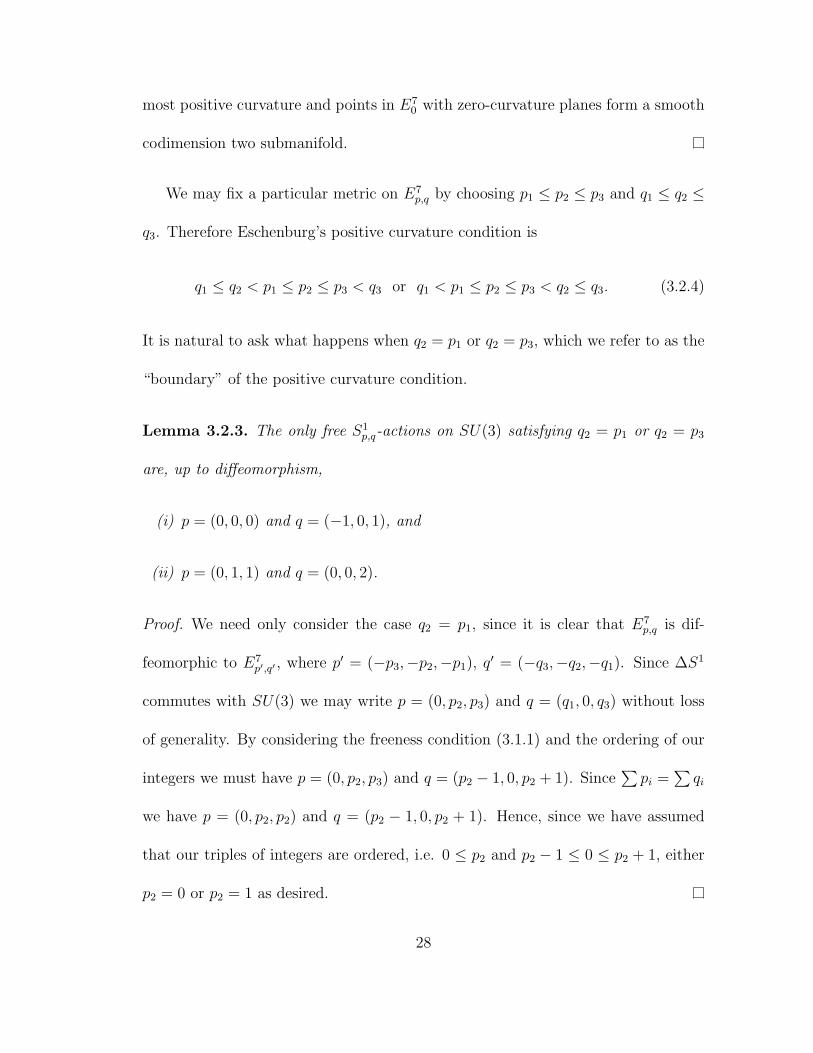
We may fix a particular metric on E7p,q by choosing p1 ≤ p2 ≤ p3 and q1 ≤ q2 ≤

q3. Therefore Eschenburg’s positive curvature condition is

q1 ≤ q2 < p1 ≤ p2 ≤ p3 < q3 or q1 < p1 ≤ p2 ≤ p3 < q2 ≤ q3. (3.2.4)

It is natural to ask what happens when q2 = p1 or q2 = p3, which we refer to as the

“boundary” of the positive curvature condition.

Lemma 3.2.3. The only free S1p,q-actions on SU(3) satisfying q2 = p1 or q2 = p3

are, up to diffeomorphism,

(i) p = (0, 0, 0) and q = (−1, 0, 1), and

(ii) p = (0, 1, 1) and q = (0, 0, 2).

Proof. We need only consider the case q2 = p1, since it is clear that E7p,q is dif-

feomorphic to E7p′,q′ , where p′ = (−p3,−p2,−p1), q′ = (−q3,−q2,−q1). Since ∆S1

commutes with SU(3) we may write p = (0, p2, p3) and q = (q1, 0, q3) without loss

of generality. By considering the freeness condition (3.1.1) and the ordering of our

integers we must have p = (0, p2, p3) and q = (p2 − 1, 0, p2 + 1). Since∑

pi =∑

qi

we have p = (0, p2, p2) and q = (p2 − 1, 0, p2 + 1). Hence, since we have assumed

that our triples of integers are ordered, i.e. 0 ≤ p2 and p2 − 1 ≤ 0 ≤ p2 + 1, either

p2 = 0 or p2 = 1 as desired.

28

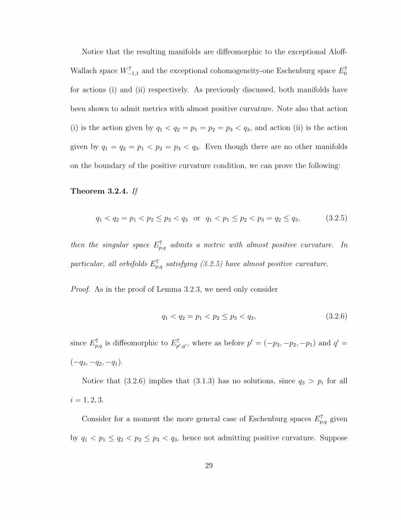
Notice that the resulting manifolds are diffeomorphic to the exceptional Aloff-

Wallach space W 7−1,1 and the exceptional cohomogeneity-one Eschenburg space E7

0

for actions (i) and (ii) respectively. As previously discussed, both manifolds have

been shown to admit metrics with almost positive curvature. Note also that action

(i) is the action given by q1 < q2 = p1 = p2 = p3 < q3, and action (ii) is the action

given by q1 = q2 = p1 < p2 = p3 < q3. Even though there are no other manifolds

on the boundary of the positive curvature condition, we can prove the following:

Theorem 3.2.4. If

q1 < q2 = p1 < p2 ≤ p3 < q3 or q1 < p1 ≤ p2 < p3 = q2 ≤ q3, (3.2.5)

then the singular space E7p,q admits a metric with almost positive curvature. In

particular, all orbifolds E7p,q satisfying (3.2.5) have almost positive curvature.

Proof. As in the proof of Lemma 3.2.3, we need only consider

q1 < q2 = p1 < p2 ≤ p3 < q3, (3.2.6)

since E7p,q is diffeomorphic to E7

p′,q′ , where as before p′ = (−p3,−p2,−p1) and q′ =

(−q3,−q2,−q1).

Notice that (3.2.6) implies that (3.1.3) has no solutions, since q3 > pi for all

i = 1, 2, 3.

Consider for a moment the more general case of Eschenburg spaces E7p,q given

by q1 < p1 ≤ q2 < p2 ≤ p3 < q3, hence not admitting positive curvature. Suppose

29

that there is a k ∈ K such that Adk Y1 is horizontal at some A ∈ SU(3). Then

(3.1.4) implies that

p1 ≤3∑

j=1

|(Ak)j1|2pj = |k11|2q1 + |k21|2q2 ≤ q2.

Since |k11|2 + |k21|2 = 1 we thus have

p1 ≤ |k11|2(q1 − q2) + q2 ≤ q2 and p1 ≤ q1 + |k21|2(q2 − q1) ≤ q2,

which are equivalent to

0 ≤ |k11|2 ≤ q2 − p1

q2 − q1

andp1 − q1

q2 − q1

≤ |k21|2 ≤ 1.

In particular, when the hypothesis of the theorem is satisfied, namely p1 = q2, we

get |k11|2 = 0 and |k21|2 = 1, i.e.

k =

0 k12 0

k21 0 0

0 0 −k12k21

∈ K = U(2).

Hence (3.1.4) becomes

|a12|2p1 + |a22|2p2 + |a32|2p3 = q2 = p1

⇐⇒ |a22|2(p2 − p1) + |a32|2(p3 − p1) = 0, since A ∈ SU(3)

⇐⇒ a22 = a32 = 0, since p1 < p2 ≤ p3

⇐⇒ A =

0 a12 0

a21 0 a23

a31 0 a33

∈ SU(3).

The set of such A ∈ SU(3) is preserved under the S1p,q-action, hence projects to a

set of measure zero in E7p,q. Therefore E7

p,q has almost positive curvature.

30

We may also examine how large the set of zero-curvature planes is at each point

of the set

S1p,q ? A

∣∣∣ A =(

0 a12 0a21 0 a23a31 0 a33

)⊂ E7

p,q, with q1 < q2 = p1 < p2 ≤ p3 < q3.

This is equivalent to determining how large the set of horizontal zero-curvature

planes is at each A =(

0 a12 0a21 0 a23a31 0 a33

)∈ SU(3).

Proposition 3.2.5. If q1 < q2 = p1 < p2 ≤ p3 < q3 then there is a one-dimensional

family of horizontal zero-curvature planes at each point A =(

0 a12 0a21 0 a23a31 0 a33

)∈ SU(3).

Proof. Recall we have shown in the proof of Theorem 3.2.4 that Y3 is never hori-

zontal, and Adk Y1 being horizontal at A implies that k =

(0 k12 0

k21 0 0

0 0 −k12k21

)∈ K =

U(2). Hence Adk Y1 = Y2 := i(

1−2

1

).

Let Y = Φ−1(Y2), where 〈X, Z〉1 = 〈X, Φ(Z)〉0. Let X ∈ HA be such that

Span X, Y is a horizontal zero-curvature plane. Then, by Lemma 2.2.2 and since

Φ−1(Y2) = 1λY2 ∈ k, [X,Y ] = [Xk, Y ] = 0, which is equivalent to

[X, Y2] = [Xk, Y2] = 0

⇐⇒ [X, Y2] = 0

⇐⇒ X =

is 0 x

0 it 0

−x 0 −i(s + t)

,

where s, t ∈ R, x ∈ C. We may assume without loss of generality that 〈X, Y 〉1 = 0.

Hence

X =

is 0 x

0 0 0

−x 0 −is

.

The set of such X is 3-dimensional. We also require that X is horizontal, i.e.

〈X, AdA∗ P−Q〉1 = 0, and without loss of generality we may assume that ||X||2 = 1.

31

Thus, for each A =(

0 a12 0a21 0 a23a31 0 a33

)∈ SU(3) there is a one-dimensional family of

horizontal zero-curvature planes Span X,Y .

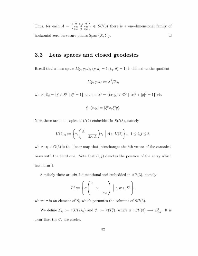
3.3 Lens spaces and closed geodesics

Recall that a lens space L(p, q; d), (p, d) = 1, (q, d) = 1, is defined as the quotient

L(p, q; d) := S3/Zd,

where Zd = ξ ∈ S1 | ξd = 1 acts on S3 = (x, y) ∈ C2 | |x|2 + |y|2 = 1 via

ξ · (x.y) = (ξpx, ξqy).

Now there are nine copies of U(2) embedded in SU(3), namely

U(2)ij :=

τi

(A

det A

)τj

∣∣∣ A ∈ U(2)

, 1 ≤ i, j ≤ 3,

where τ` ∈ O(3) is the linear map that interchanges the `th vector of the canonical

basis with the third one. Note that (i, j) denotes the position of the entry which

has norm 1.

Similarly there are six 2-dimensional tori embedded in SU(3), namely

T 2σ :=

σ

z

w

zw

∣∣∣ z, w ∈ S1

,

where σ is an element of S3 which permutes the columns of SU(3).

We define Lij := π(U(2)ij) and Cσ := π(T 2σ ), where π : SU(3) −→ E7

p,q. It is

clear that the Cσ are circles.

32

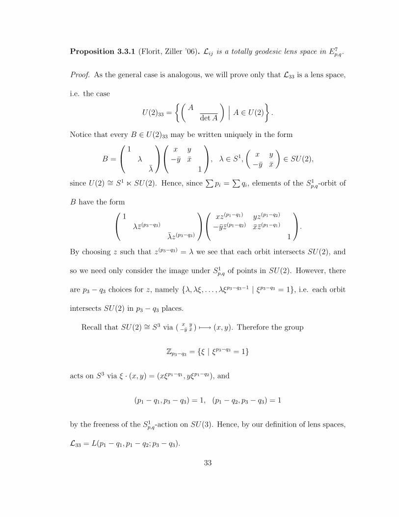
Proposition 3.3.1 (Florit, Ziller ’06). Lij is a totally geodesic lens space in E7p,q.

Proof. As the general case is analogous, we will prove only that L33 is a lens space,

i.e. the case

U(2)33 =

(A

det A

) ∣∣∣ A ∈ U(2)

.

Notice that every B ∈ U(2)33 may be written uniquely in the form

B =

1

λ

λ

x y

−y x

1

, λ ∈ S1,

(x y

−y x

)∈ SU(2),

since U(2) ∼= S1 n SU(2). Hence, since∑

pi =∑

qi, elements of the S1p,q-orbit of

B have the form

1

λz(p3−q3)

λz(p3−q3)

xz(p1−q1) yz(p1−q2)

−yz(p1−q2) xz(p1−q1)

1

.

By choosing z such that z(p3−q3) = λ we see that each orbit intersects SU(2), and

so we need only consider the image under S1p,q of points in SU(2). However, there

are p3 − q3 choices for z, namely λ, λξ, . . . , λξp3−q3−1 | ξp3−q3 = 1, i.e. each orbit

intersects SU(2) in p3 − q3 places.

Recall that SU(2) ∼= S3 via (x y−y x ) 7−→ (x, y). Therefore the group

Zp3−q3 = ξ | ξp3−q3 = 1

acts on S3 via ξ · (x, y) = (xξp1−q1 , yξp1−q2), and

(p1 − q1, p3 − q3) = 1, (p1 − q2, p3 − q3) = 1

by the freeness of the S1p,q-action on SU(3). Hence, by our definition of lens spaces,

L33 = L(p1 − q1, p1 − q2; p3 − q3).

33

In order to prove that Lij is totally geodesic in E7p,q we first assume that U(2)ij

is totally geodesic in SU(3) (with respect to 〈 , 〉1). A geodesic γ in Lij lifts to

a horizontal geodesic γ in U(2)ij, since S1p,q ? A ⊂ U(2)i,j for all A ∈ U(2)ij and

γ′(0) ⊥ S1p,q ? γ(0).

Now, since we assumed that U(2)ij is totally geodesic, this implies that γ is

a horizontal geodesic in SU(3). Hence γ projects to a geodesic in E7p,q, which by

uniqueness must be γ. Thus Lij is totally geodesic in E7p,q.

It remains to show that U(2)ij is totally geodesic in SU(3). Consider isometries

of SU(3) given by A 7−→ zr · A · zrσ , where

zr :=

zr1

zr2

zr3

with two of r1, r2, r3 equal, and

zrσ :=

zrσ(1)

zrσ(2)

zrσ(3)

, σ ∈ S3.

Each U(2)ij is the fixed point set of such an isometry and hence totally geodesic in

SU(3).

Now notice that the circles Cσ are the intersections of two totally geodesic sub-

manifolds. Hence we have immediately

Corollary 3.3.2. Cσ is a closed geodesic in E7p,q.

We can arrange the lens spaces and closed geodesics in the following schematic

34

diagram

Cid

L11

uuuuuuuuu

L22

L33

IIIIIIIII

C(2 3)

L23

LLLLLLLLLL

L32

LLLLLLLLLL

C(1 2)

rrrrrrrrrrL12

rrrrrrrrrr L21

C(1 2 3)

L31 IIIIIIIIIC(1 3 2)

L13uuuuuuuuu

C(1 3)

Suppose now that we fix a metric on an Eschenburg space E7p,q by specifying

p1 ≤ p2 ≤ p3 and q1 ≤ q2 ≤ q3. By again examining equations (3.1.3) and (3.1.4) we

can find conditions under which all of the points in each of the nine lens spaces Lij

and each of the six closed geodesics Cσ admit positive curvature. These conditions

are collected in Tables 3.1 and 3.2.

As an example, if we assume that p1 > q1 and p2 > q2, then we have positive

curvature on L11,L22 and L32 (and hence on Cid, C(2 3), C(1 3 2) and C(1 3)). With the

extra assumption that q2 < 0 < p2 we get positive curvature on L13. However we

get positive curvature on the remaining lens spaces if and only if q2 < p1, i.e.

q1 ≤ q2 < p1 ≤ p2 ≤ p3 < q3, q2 < 0 < p2,

in which case the entire manifold E7p,q (where we have assumed the action is free)

has positive curvature, by Theorem 3.1.2.

Notice that, in particular, the “worst” lens space when p1 > q1 and p2 > q2, i.e.

the lens space containing no points of positive curvature, is exactly the lens space

35

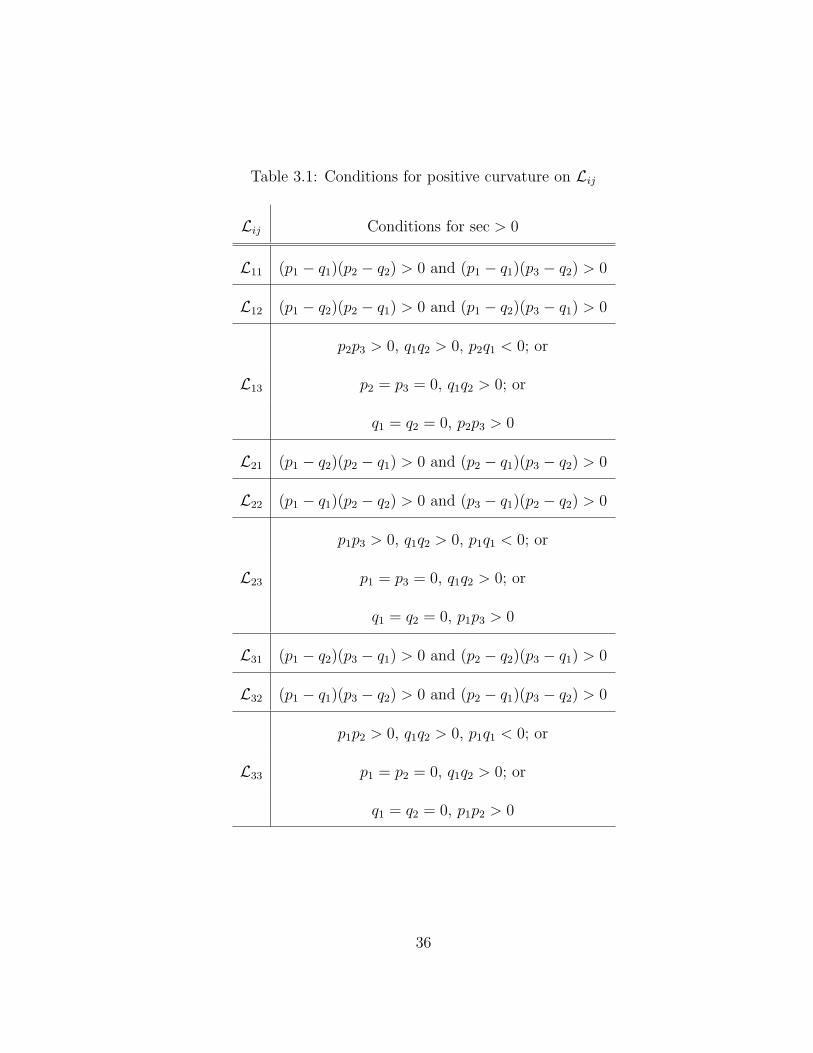
Table 3.1: Conditions for positive curvature on Lij

Lij Conditions for sec > 0

L11 (p1 − q1)(p2 − q2) > 0 and (p1 − q1)(p3 − q2) > 0

L12 (p1 − q2)(p2 − q1) > 0 and (p1 − q2)(p3 − q1) > 0

p2p3 > 0, q1q2 > 0, p2q1 < 0; or

L13 p2 = p3 = 0, q1q2 > 0; or

q1 = q2 = 0, p2p3 > 0

L21 (p1 − q2)(p2 − q1) > 0 and (p2 − q1)(p3 − q2) > 0

L22 (p1 − q1)(p2 − q2) > 0 and (p3 − q1)(p2 − q2) > 0

p1p3 > 0, q1q2 > 0, p1q1 < 0; or

L23 p1 = p3 = 0, q1q2 > 0; or

q1 = q2 = 0, p1p3 > 0

L31 (p1 − q2)(p3 − q1) > 0 and (p2 − q2)(p3 − q1) > 0

L32 (p1 − q1)(p3 − q2) > 0 and (p2 − q1)(p3 − q2) > 0

p1p2 > 0, q1q2 > 0, p1q1 < 0; or

L33 p1 = p2 = 0, q1q2 > 0; or

q1 = q2 = 0, p1p2 > 0

36

Table 3.2: Conditions for positive curvature on Cσ

Cσ Condition for sec > 0

Cid (p1 − q1)(p2 − q2) > 0

C(1 2) (p1 − q2)(p2 − q1) > 0

C(1 3) (p3 − q1)(p2 − q2) > 0

C(2 3) (p1 − q1)(p3 − q2) > 0

C(1 2 3) (p1 − q2)(p3 − q1) > 0

C(1 3 2) (p2 − q1)(p3 − q2) > 0

L12 which arises as the set of points admitting zero-curvature planes in the case

q1 < q2 = p1 < p2 ≤ p3 < q3, of which there are only singular examples, and these

examples admit almost positive curvature.

37

Chapter 4

Bazaikin Spaces

4.1 Positive curvature

The proof of positive curvature on an infinite subfamily of the Bazaikin spaces

follows from essentially the same techniques as in the case of the Eschenburg spaces.

We recall the proof as given in [Zi1], with a slight modification which will allow us

to prove the results in Theorem A(iii) and (iv).

Recall that the Bazaikin spaces are defined as

B13q1,...,q5

:= SU(5)//Sp(2) · S1q1,...,q5

,

where q1, . . . , q5 ∈ Z, and

Sp(2) · S1q1,...,q5

= (Sp(2)× S1q1,...,q5

)/Z2, Z2 = ±(1, I),

38

acts effectively on SU(5) via

[A, z] ? B =

zq1

. . .

zq5

B

(A

zq

),

with z ∈ S1, A ∈ Sp(2) → SU(4), B ∈ SU(5), and q =∑

qi. We recall that

Sp(2) → SU(4)

A = S + Tj 7−→ A =

(S T

−T S

).

It is not difficult to show that the action of Sp(2) · S1q1,...,q5

is free if and only all

q1, . . . , q5 are odd and (qσ(1) + qσ(2), qσ(3) + qσ(4)) = 2 for all σ ∈ S5.

Let G = SU(5) ⊃ K = U(4), where K → G via

A 7−→(

A

det A

).

Then (G, K) is a rank one symmetric pair, with Lie algebras (g, k). With respect

to the bi-invariant metric 〈X,Y 〉0 = −Re tr XY we may write g = k ⊕ p. Define

a metric, 〈 , 〉1, on G as in 2.2.1 which is left-invariant and right K-invariant. In

particular we have 〈X, Y 〉1 = 〈X, Φ(Y )〉0, where Φ(Y ) = Yp + λYk, λ ∈ (0, 1). By

Lemma 2.2.2 we know that a plane σ = Span Φ−1(X), Φ−1(Y ) ⊂ g has zero-

curvature with respect to 〈 , 〉1 if and only if

0 = [X,Y ] = [Xp, Yp] = [Xk, Yk].

It is clear that the action of U := Sp(2) ·S1q1,...,q5

is by isometries since U is contained

in SU(5)×U(4) ⊂ SU(5)×SU(5). Therefore we get an induced submersion metric

on B13q1,...,q5

= G//U .

39

Since 〈 , 〉1 is left-invariant we may left-translate back to the Lie algebra g

without changing our computations. Therefore the vertical subspace at A ∈ SU(5)

with respect to the U -action may be written as

VA =

θ AdA∗ Q−

(X

iθq

) ∣∣∣ θ ∈ R, Q = i

( q1

...q5

), X ∈ sp(2) ⊂ su(4)

where A∗ = At. Our aim is to determine when zero-curvature planes with respect

to 〈 , 〉1 are horizontal at A ∈ SU(5). A vector Φ−1(X) is orthogonal to VA with

respect to 〈 , 〉1 if and only if

⟨X, AdA∗ Q−

(0

00

0iq

)⟩

0

= 0 and X ⊥0 sp(2) ⊂ su(4), (4.1.1)

where ⊥0 denotes orthogonality with respect to 〈 , 〉0.

Lemma 4.1.1. σ = Span Φ−1(X), Φ−1(Y ) ⊂ g is a horizontal zero-curvature

plane with respect to 〈 , 〉1 if and only if either

W1 := diag(i, i, i, i,−4i) or W2 := Adk diag(2i,−3i, 2i,−3i, 2i),

for some k ∈ Sp(2), is in σ and is horizontal.

Proof. Suppose that σ = Span Φ−1(X), Φ−1(Y ) has zero-curvature with respect

to 〈 , 〉1. Then, since [Xp, Yp] = 0 by Lemma 2.2.2, we may assume without loss of

generality that Yp = 0, i.e X = Xp + Xk, Y = Yk.

If we also have Xp = 0, then X, Y ∈ k. Notice that k = z ⊕ sp(2) ⊕ m, where

z ⊥ su(4) is the centre of k, generated by diag(i, i, i, i,−4i), and m = sp(2)⊥ ⊂ su(4).

But we have assumed that X, Y ⊥0 sp(2). Thus X,Y ∈ z⊕m, and [X,Y ] = 0 if and

40

only if [Xm, Ym] = 0. Now SU(4) = Spin(6), Sp(2) = Spin(5) and (SU(4), Sp(2))

is a rank one symmetric pair. Therefore Xm, Ym must be linearly dependent and

we may assume without loss of generality that X = Xm, Y = Yz. Then z ⊂ σ, i.e.

W1 = diag(i, i, i, i,−4i) ∈ σ.

We now note that W1 being horizontal is not only a necessary condition for

σ ⊂ k to be a horizontal zero-curvature plane, but also sufficient for the existence

of such a plane as, for dimension reasons, we may always find a vector X ∈ m such

that σ = Span Φ−1(X), Φ−1(W1) is a horizontal zero-curvature plane.

On the other hand, suppose now that Xp 6= 0. Then the conditions for zero-

curvature become 0 = [Xp, Yk] = [Xk, Yk]. Suppose that

Xp =

(0 x

−xt 0

), Y = Yk =

(Z

− tr Z

),

where x ∈ C4 and Z ∈ u(4) = z ⊕ su(4). Then 0 = [Xp, Yk] if and only if

Zx = −(tr Z)x. Let Z = itI + Z ′ ∈ z ⊕ su(4), t ∈ R. Since it is required

that Y ⊥ sp(2) we have Z ′ ⊥ sp(2) ⊂ su(4). Recall that SU(4) = Spin(6),

Sp(2) = Spin(5). Therefore SU(4)/Sp(2) = S5 and, since Sp(2) = Spin(5) acts

transitively on distance spheres in m = sp(2)⊥ ⊂ su(4), we may write

Z ′ = k

is

−is

is

−is

k−1, k ∈ Sp(2).

This in turn implies that Z may be written as

Z = k

i(t + s)

i(t− s)

i(t + s)

i(t− s)

k−1, k ∈ Sp(2).

41

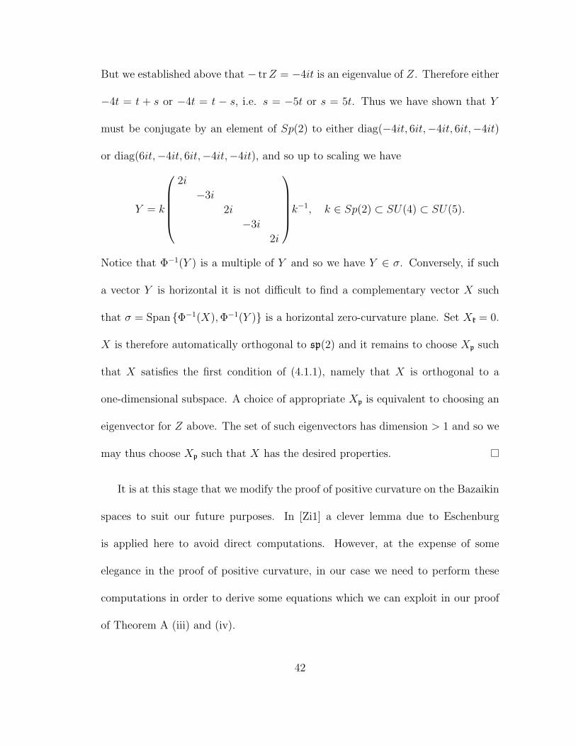
But we established above that − tr Z = −4it is an eigenvalue of Z. Therefore either

−4t = t + s or −4t = t − s, i.e. s = −5t or s = 5t. Thus we have shown that Y

must be conjugate by an element of Sp(2) to either diag(−4it, 6it,−4it, 6it,−4it)

or diag(6it,−4it, 6it,−4it,−4it), and so up to scaling we have

Y = k

2i

−3i

2i

−3i

2i

k−1, k ∈ Sp(2) ⊂ SU(4) ⊂ SU(5).

Notice that Φ−1(Y ) is a multiple of Y and so we have Y ∈ σ. Conversely, if such

a vector Y is horizontal it is not difficult to find a complementary vector X such

that σ = Span Φ−1(X), Φ−1(Y ) is a horizontal zero-curvature plane. Set Xk = 0.

X is therefore automatically orthogonal to sp(2) and it remains to choose Xp such

that X satisfies the first condition of (4.1.1), namely that X is orthogonal to a

one-dimensional subspace. A choice of appropriate Xp is equivalent to choosing an

eigenvector for Z above. The set of such eigenvectors has dimension > 1 and so we

may thus choose Xp such that X has the desired properties.

It is at this stage that we modify the proof of positive curvature on the Bazaikin

spaces to suit our future purposes. In [Zi1] a clever lemma due to Eschenburg

is applied here to avoid direct computations. However, at the expense of some

elegance in the proof of positive curvature, in our case we need to perform these

computations in order to derive some equations which we can exploit in our proof

of Theorem A (iii) and (iv).

42

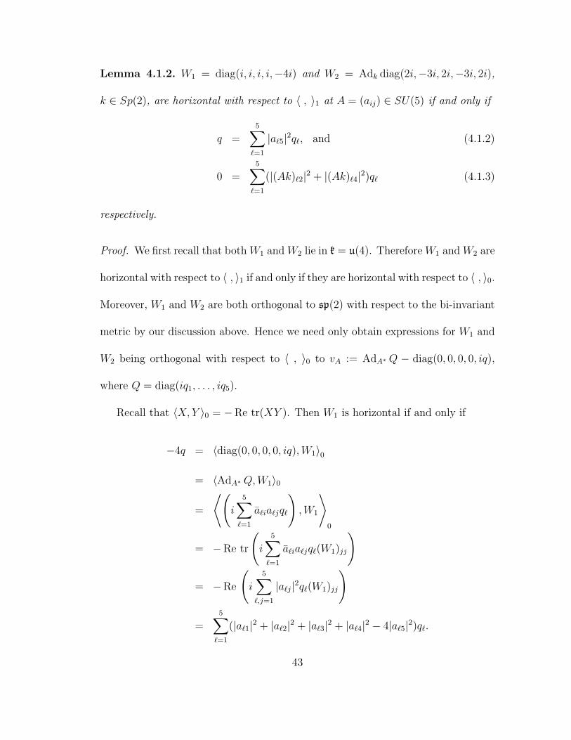
Lemma 4.1.2. W1 = diag(i, i, i, i,−4i) and W2 = Adk diag(2i,−3i, 2i,−3i, 2i),

k ∈ Sp(2), are horizontal with respect to 〈 , 〉1 at A = (aij) ∈ SU(5) if and only if

q =5∑

`=1

|a`5|2q`, and (4.1.2)

0 =5∑

`=1

(|(Ak)`2|2 + |(Ak)`4|2)q` (4.1.3)

respectively.

Proof. We first recall that both W1 and W2 lie in k = u(4). Therefore W1 and W2 are

horizontal with respect to 〈 , 〉1 if and only if they are horizontal with respect to 〈 , 〉0.

Moreover, W1 and W2 are both orthogonal to sp(2) with respect to the bi-invariant

metric by our discussion above. Hence we need only obtain expressions for W1 and

W2 being orthogonal with respect to 〈 , 〉0 to vA := AdA∗ Q − diag(0, 0, 0, 0, iq),

where Q = diag(iq1, . . . , iq5).

Recall that 〈X, Y 〉0 = −Re tr(XY ). Then W1 is horizontal if and only if

−4q = 〈diag(0, 0, 0, 0, iq),W1〉0

= 〈AdA∗ Q, W1〉0

=

⟨(i

5∑

`=1

a`ia`jq`

),W1

⟩

0

= −Re tr

(i

5∑

`=1

a`ia`jq`(W1)jj

)

= −Re

(i

5∑

`,j=1

|a`j|2q`(W1)jj

)

=5∑

`=1

(|a`1|2 + |a`2|2 + |a`3|2 + |a`4|2 − 4|a`5|2)q`.

43

Now using the fact that A is unitary together with q =∑5

`=1 q` yields

−4q =5∑

`=1

((1− |a`5|2)− 4|a`5|2)q`

=5∑

`=1

(1− 5|a`5|2)q`

= q − 55∑

`=1

|a`5|2q`

as desired.

Consider now W2 = Adk W , where W = diag(2i,−3i, 2i,−3i, 2i). Then W2 is

horizontal if and only if

2q =⟨diag(0, 0, 0, 0, iq), W

⟩0

=⟨Adk∗ diag(0, 0, 0, 0, iq), W

⟩0

for k ∈ Sp(2) ⊂ SU(4)

= 〈diag(0, 0, 0, 0, iq),W2〉0

= 〈AdA∗ Q, W2〉0

=⟨Ad(Ak)∗ Q, W

⟩0

=

⟨(i

5∑

`=1

(Ak)`i(Ak)`jq`

), W

⟩

0

= −Re tr

(i

5∑

`=1

(Ak)`i(Ak)`jq`(W )jj

)

= −Re

(i

5∑

`,j=1

|(Ak)`j|2q`(W )jj

)

=5∑

`=1

(2|(Ak)`1|2 − 3|(Ak)`2|2 + 2|(Ak)`3|2 − 3|(Ak)`4|2 + 2|(Ak)`5|2

)q`

=5∑

`=1

(2− 5

(|(Ak)`2|2 + |(Ak)`4|2))

q`, since A is unitary.

44

Equation (4.1.3) now follows immediately from q =∑5

`=1 q`.

We may now state the conditions for a Bazaikin space to admit positive curva-

ture.

Theorem 4.1.3. The Bazaikin space B13q1,...,q5

= (SU(5), 〈 , 〉1)//S1q1,...,q5

· Sp(2)

admits positive sectional curvature if and only if

qσ(1) + qσ(2) > 0 (or < 0) for all permutations σ ∈ S5. (4.1.4)

Proof. Suppose qσ(1) + qσ(2) > 0 for all permutations σ ∈ S5. In particular notice

that this implies that q > 0. Through Lemmas 4.1.1 and 4.1.2 we have established

that we need only examine equations (4.1.2) and (4.1.3) to obtain the desired result.

Consider equation (4.1.2) in the alternative form

5∑

`=1

(1− |a`5|2)q` = 0.

Since A ∈ SU(5) is unitary we know that either 1 − |a`5|2 6= 0 for all ` = 1, . . . , 5,

or 1− |a`05|2 = 0 for exactly one `0 ∈ 1, . . . , 5. In the first case we have, for some

`0 ∈ 1, . . . , 5,5∑

`=1

(1− |a`5|2)q` ≥ (1− |a`05|2)5∑

`=1

q` = (1− |a`05|2)q > 0,

and so there are no solutions to equation (4.1.2). In the second case equation (4.1.2)

reduces to, without loss of generality, q1 = q. Thus in order to have solutions we

require q2 + q3 + q4 + q5 = 0, which is impossible by our hypothesis. Hence we have

established that there can be no solutions to equation (4.1.2).

45

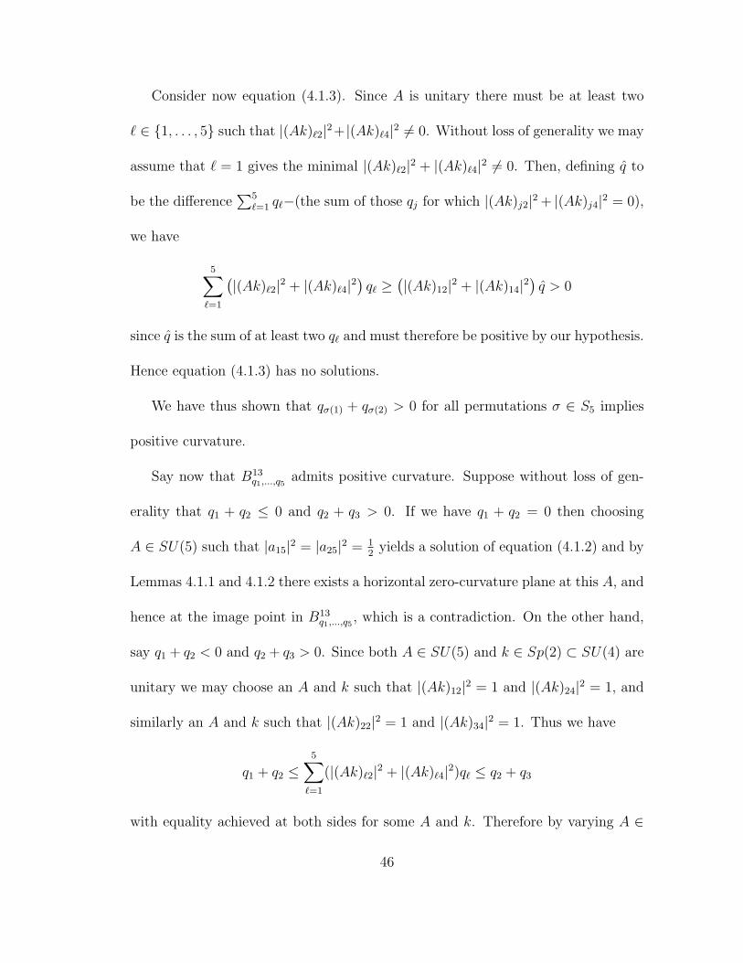
Consider now equation (4.1.3). Since A is unitary there must be at least two

` ∈ 1, . . . , 5 such that |(Ak)`2|2+|(Ak)`4|2 6= 0. Without loss of generality we may

assume that ` = 1 gives the minimal |(Ak)`2|2 + |(Ak)`4|2 6= 0. Then, defining q to

be the difference∑5

`=1 q`−(the sum of those qj for which |(Ak)j2|2 + |(Ak)j4|2 = 0),

we have

5∑

`=1

(|(Ak)`2|2 + |(Ak)`4|2)q` ≥

(|(Ak)12|2 + |(Ak)14|2)q > 0

since q is the sum of at least two q` and must therefore be positive by our hypothesis.

Hence equation (4.1.3) has no solutions.

We have thus shown that qσ(1) + qσ(2) > 0 for all permutations σ ∈ S5 implies

positive curvature.

Say now that B13q1,...,q5

admits positive curvature. Suppose without loss of gen-

erality that q1 + q2 ≤ 0 and q2 + q3 > 0. If we have q1 + q2 = 0 then choosing

A ∈ SU(5) such that |a15|2 = |a25|2 = 12

yields a solution of equation (4.1.2) and by

Lemmas 4.1.1 and 4.1.2 there exists a horizontal zero-curvature plane at this A, and

hence at the image point in B13q1,...,q5

, which is a contradiction. On the other hand,

say q1 + q2 < 0 and q2 + q3 > 0. Since both A ∈ SU(5) and k ∈ Sp(2) ⊂ SU(4) are

unitary we may choose an A and k such that |(Ak)12|2 = 1 and |(Ak)24|2 = 1, and

similarly an A and k such that |(Ak)22|2 = 1 and |(Ak)34|2 = 1. Thus we have

q1 + q2 ≤5∑

`=1

(|(Ak)`2|2 + |(Ak)`4|2)q` ≤ q2 + q3

with equality achieved at both sides for some A and k. Therefore by varying A ∈

46

SU(5) and k ∈ Sp(2) continuously we may obtain a solution to equation (4.1.3)

and hence a zero-curvature plane by Lemmas 4.1.1 and 4.1.2.

4.2 Almost and quasi-positive curvature

Consider a general Bazaikin space B13q1,...,q5

. Since each qj is odd, it is clear that at

least three of the qj must have the same sign. Suppose that four of the qj share

the same sign. By the discussion in §2.1 we may assume without loss of generality

that q1, . . . , q4 are all positive. We remark that by Theorem 4.1.3 we get positive

curvature if qj + q5 > 0 for all j = 1, . . . , 4. We are now in a position to prove

Theorem A (iii).

Theorem 4.2.1. All B13q1,...,q5

with q1, . . . , q4 > 0 admit quasi-positive curvature.

Proof. As we established in Lemmas 4.1.1 and 4.1.2, there is a horizontal zero-

curvature plane at A ∈ SU(5) if and only if we can solve either equation (4.1.2)

or equation (4.1.3) at A. If we allow A to be diagonal then equations (4.1.2) and

(4.1.3) become

q5 =5∑

`=1

q`, and (4.2.1)

0 =5∑

`=1

(|k`2|2 + |k`4|2)q` (4.2.2)

respectively. By hypothesis q1, . . . , q4 > 0 and therefore equality in (4.2.1) is im-

possible. On the other hand, because of how we have embedded Sp(2) in SU(5),

47

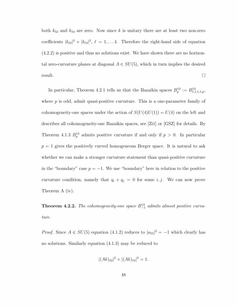
both k52 and k54 are zero. Now since k is unitary there are at least two non-zero

coefficients |k`2|2 + |k`4|2, ` = 1, . . . 4. Therefore the right-hand side of equation

(4.2.2) is positive and thus no solutions exist. We have shown there are no horizon-

tal zero-curvature planes at diagonal A ∈ SU(5), which in turn implies the desired

result.

In particular, Theorem 4.2.1 tells us that the Bazaikin spaces B13p := B13

1,1,1,1,p,

where p is odd, admit quasi-positive curvature. This is a one-parameter family of

cohomogeneity-one spaces under the action of S(U(4)U(1)) = U(4) on the left and

describes all cohomogeneity-one Bazaikin spaces, see [Zi1] or [GSZ] for details. By

Theorem 4.1.3 B13p admits positive curvature if and only if p > 0. In particular

p = 1 gives the positively curved homogeneous Berger space. It is natural to ask

whether we can make a stronger curvature statement than quasi-positive curvature

in the “boundary” case p = −1. We use “boundary” here in relation to the positive

curvature condition, namely that qi + qj = 0 for some i, j. We can now prove

Theorem A (iv).

Theorem 4.2.2. The cohomogeneity-one space B13−1 admits almost positive curva-

ture.

Proof. Since A ∈ SU(5) equation (4.1.2) reduces to |a55|2 = −1 which clearly has

no solutions. Similarly equation (4.1.3) may be reduced to

|(Ak)52|2 + |(Ak)54|2 = 1.

48

Since Ak is unitary this implies that |(Ak)51|2 = |(Ak)53|2 = |(Ak)55|2 = 0. In

particular we have (Ak)55 = 0. But (Ak)55 = a55k55 because of our embedding

of Sp(2) in SU(5), and for the same reason |k55| = 1. Hence a55 = 0, and so

B13−1 has almost positive curvature since this is clearly invariant under the action of

S1q1,··· ,q5

· Sp(2).

As it turns out, we may apply a result of Taimanov [T] to show that the Bazaikin

space B13−1 contains two interesting totally geodesic submanifolds.

Proposition 4.2.3. B13−1 contains the exceptional Aloff-Wallach space W 7

−1,1 and

the exceptional cohomogeneity-one Eschenburg space E70 as totally geodesic subman-

ifolds.

Proof. Let σ = diag(−1,−1, 1, 1, 1) ∈ SU(5). σ acts on SU(5) via conjugation, and

hence induces an action on a general Bazaikin space B13q1,...,q5

. The induced action is

given by σ ? [A] = [σ ? A], for A ∈ SU(5), [A] ∈ B13q1,...,q5

, since conjugation by σ is

in the normalizer of Sp(2) ⊂ SU(5). Clearly the σ-action on B13q1,...,q5

is an isometry.

Recall that each component of the fixed point set of an isometry is a totally geodesic

submanifold. Taimanov shows in [T] that one component of Fix(σ), the fixed point

set of the σ-action, is given by

Fix(σ)0 := S(U(2)U(3))//(U(2) · S1q1,...,q5

) ⊂ B13q1,...,q5

,

where the U(2) in U(2) · S1q1,...,q5

is the usual embedding of U(2) into Sp(2). In

fact Taimanov shows that Fix(σ)0 is isometric to the Eschenburg space E7a,b with

49

a = (q3, q4, q5) and b = (−q1,−q2, q), where we recall that q =∑

qi.

Thus we immediately see that B13−1 = B13

1,1,1,1,−1 contains the Eschenburg space

described by a = (1, 1,−1), b = (−1,−1, 3) as a totally geodesic submanifold.

However this is none other than E70 in disguise, where E7

0 is the Eschenburg space

described by a = (1, 1, 0), b = (0, 0, 2).

On the other hand, recall from §2.1 that we may conjugate the left-hand side of

the action of Sp(2) ·S1q1,...,q5

by some element of SU(5) to get an isometric Bazaikin

space. Let g ∈ SU(5) be an element which permutes the entries on the diagonal of

the left-hand side of the action of Sp(2) · S1q1,...,q5

, namely g diag(z, z, z, z, z)g−1 =

diag(z, z, z, z, z). Let fg : B131,1,1,1,−1 −→ B13

−1,1,1,1,1 be the resulting isometry. By

the results of Taimanov B13−1,1,1,1,1 contains the Eschenburg space described by a =

(1, 1, 1), b = (1,−1, 3) as a totally geodesic submanifold. However again we notice

that this is none other than the Aloff-Wallach space W 7−1,1 described by a = (0, 0, 0),

b = (0,−1, 1). Now since fg is an isometry we see that f−1g (W 7

−1,1)∼= W 7

−1,1 is a

totally geodesic submanifold of B13−1 as desired.

As we mentioned in the introduction, W 7−1,1 has a zero-curvature plane at every

point, whereas we showed in Theorem 3.2.2 that E70 has almost positive curvature.

50

Chapter 5

Quotients of S7 × S7

5.1 The Cayley numbers, G2 and its Lie algebra

We recall without proof some well known facts about Cayley numbers, the Lie group

G2 and its Lie algebra. More details may be found in [GWZ] and [M].

We may write the Cayley numbers as Ca = H + H`. Thus we have a natural

orthonormal basis

e0 = 1, e1 = i, e2 = j, e3 = k, e4 = `, e5 = i`, e6 = j`, e7 = k`

for Ca. Note that this description of Ca differs slightly from that given in [M]. This

will account for the difference in the descriptions of the Lie algebra g2. Multiplica-

tion in Ca is non-associative and defined via

(a + b`)(c + d`) = (ac− db) + (da + bc)`, a, b, c, d ∈ H, (5.1.1)

51

and hence we have the following multiplication table, where the order of multipli-

cation is given by (row)∗(column):

Table 5.1: Multiplication table for Ca

e1 = i e2 = j e3 = k e4 = ` e5 = i` e6 = j` e7 = k`

e1 = i −1 k −j i` −` −k` j`

e2 = j −k −1 i j` k` −` −i`

e3 = k j −i −1 k` −j` i` −`

e4 = ` −i` −j` −k` −1 i j k

e5 = i` ` −k` j` −i −1 −k j

e6 = j` k` ` −i` −j k −1 −i

e7 = k` −j` i` ` −k −j i −1

Recall that the Lie group G2 is the automorphism group of Ca ∼= R8. In fact

G2 is a connected subgroup of SO(7) ⊂ SO(8), where SO(8) acts on Ca ∼= R8

by orthogonal transformations and SO(7) is that subgroup consisting of elements

which leave e0 = 1 fixed. SO(8) also contains two copies of Spin(7) which are not

conjugate in SO(8), and G2 is the intersection of these two subgroups.

As our eventual goal is to prove Theorem A(v) and (vi), it is useful to recall the

fact that G2 appears in the descriptions of some interesting homogeneous spaces.

The following results are well-known and we state them without proof. More details

may be found in, for example, [M], [J] (page 93).

52

Theorem 5.1.1.

(i) Spin(7)/G2 = S7, which inherits positive curvature from the bi-invariant met-

ric on Spin(7);

(ii) Spin(8)/G2 = S7 × S7 and SO(8)/G2 = (S7 × S7)/Z2, where Z2 = ±id;

(iii) G2/SU(3) = S6.

These statements follow from applications of the triality principle for SO(8).

More details may be obtained in [M]. SO(8)/G2 = (S7 × S7)/Z2 has a geometric

interpretation as the set of all possible Cayley multiplications on R8. Note that for

H we get SO(4)/SO(3) = S3 as the set of all possible quaternionic multiplications

on R4.

We now turn our attention to the Lie algebra of G2. The proof of the following

theorem follows exactly as in [M] except that we use the basis and multiplication

conventions for Ca as in Table 5.1. Recall that so(n) = A ∈ Mn(R) | At = −A.

Theorem 5.1.2. The Lie algebra of G2, denoted by g2, consists of matrices A =

(aij) ∈ so(7) which satisfy aij + aji = 0 and

a23 + a45 + a76 = 0

a12 + a47 + a65 = 0

a13 + a64 + a75 = 0

a14 + a72 + a36 = 0

a15 + a26 + a37 = 0

a16 + a52 + a43 = 0

a17 + a24 + a53 = 0.

53

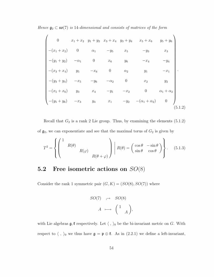
Hence g2 ⊂ so(7) is 14-dimensional and consists of matrices of the form

0 x1 + x2 y1 + y2 x3 + x4 y3 + y4 x5 + x6 y5 + y6

−(x1 + x2) 0 α1 −y5 x5 −y3 x3

−(y1 + y2) −α1 0 x6 y6 −x4 −y4

−(x3 + x4) y5 −x6 0 α2 y1 −x1

−(y3 + y4) −x5 −y6 −α2 0 x2 y2

−(x5 + x6) y3 x4 −y1 −x2 0 α1 + α2

−(y5 + y6) −x3 y4 x1 −y2 −(α1 + α2) 0

.

(5.1.2)

Recall that G2 is a rank 2 Lie group. Thus, by examining the elements (5.1.2)

of g2, we can exponentiate and see that the maximal torus of G2 is given by

T 2 =

1

R(θ)

R(ϕ)

R(θ + ϕ)

∣∣∣∣∣ R(θ) =

(cos θ − sin θ

sin θ cos θ

)

. (5.1.3)

5.2 Free isometric actions on SO(8)

Consider the rank 1 symmetric pair (G,K) = (SO(8), SO(7)) where

SO(7) → SO(8)

A 7−→(

1

A

),

with Lie algebras g, k respectively. Let 〈 , 〉0 be the bi-invariant metric on G. With

respect to 〈 , 〉0 we thus have g = p ⊕ k. As in (2.2.1) we define a left-invariant,

54

right K-invariant metric 〈 , 〉1 on G by

〈X, Y 〉1 = 〈X, Φ(Y )〉0, (5.2.1)

where Φ(Y ) = Yp + λYk, λ ∈ (0, 1). Recall that by Lemma 2.2.2 we know that a

plane

σ = Span Φ−1(X), Φ−1(Y ) ⊂ g

has zero-curvature with respect to 〈 , 〉1 if and only if

0 = [X,Y ] = [Xp, Yp] = [Xk, Yk]. (5.2.2)

We now equip G with a K-invariant metric 〈〈 , 〉〉 induced via the diffeomorphism

∆G\(G×G) −→ G

[(g1, g2)] 7−→ g−11 g2,

where G×G is equipped with the product metric 〈 , 〉1 ⊕ 〈 , 〉1.

Consider the isometric action of Up1,p2,p3 := S1p1,p2,p3

× G2 ⊂ K × K on SO(8)

defined by

A 7−→ Rp1,p2,p3(θ) · A · g−1, (5.2.3)

where A ∈ SO(8), g ∈ G2, and

Rp1,p2,p3(θ) =

I2×2

R(p1θ)

R(p2θ)

R(p3θ)

, R(θ) =

(cos θ − sin θ

sin θ cos θ

).

(5.2.4)

55

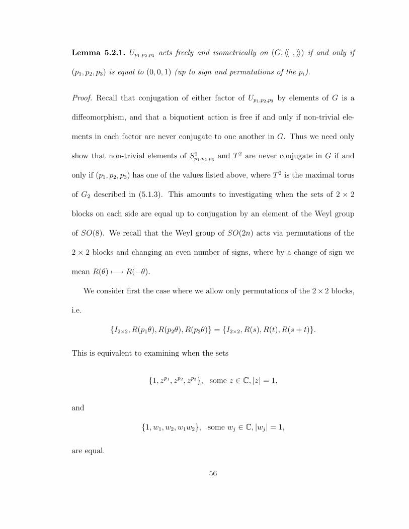
Lemma 5.2.1. Up1,p2,p3 acts freely and isometrically on (G, 〈〈 , 〉〉) if and only if

(p1, p2, p3) is equal to (0, 0, 1) (up to sign and permutations of the pi).

Proof. Recall that conjugation of either factor of Up1,p2,p3 by elements of G is a

diffeomorphism, and that a biquotient action is free if and only if non-trivial ele-

ments in each factor are never conjugate to one another in G. Thus we need only

show that non-trivial elements of S1p1,p2,p3

and T 2 are never conjugate in G if and

only if (p1, p2, p3) has one of the values listed above, where T 2 is the maximal torus

of G2 described in (5.1.3). This amounts to investigating when the sets of 2 × 2

blocks on each side are equal up to conjugation by an element of the Weyl group

of SO(8). We recall that the Weyl group of SO(2n) acts via permutations of the

2 × 2 blocks and changing an even number of signs, where by a change of sign we

mean R(θ) 7−→ R(−θ).

We consider first the case where we allow only permutations of the 2× 2 blocks,

i.e.

I2×2, R(p1θ), R(p2θ), R(p3θ) = I2×2, R(s), R(t), R(s + t).

This is equivalent to examining when the sets

1, zp1 , zp2 , zp3, some z ∈ C, |z| = 1,

and

1, w1, w2, w1w2, some wj ∈ C, |wj| = 1,

are equal.

56

Suppose 1 = 1, i.e. zp1 , zp2 , zp3 = w1, w2, w1w2. Then zpσ(1) = w1,zpσ(2) =

w2, and zpσ(3) = w1w2, some σ ∈ S3. Hence zpσ(1)+pσ(2)−pσ(3) = 1. Since z = w1 =

w2 = 1 is a necessary condition for Up1,p2,p3 to act freely, we also require that

pσ(1) + pσ(2) − pσ(3) = ±1, for all σ ∈ S3. (5.2.5)

Thus by (5.2.5) if we are to have a free action we require that

p1 + p2 − p3 = ±1, (5.2.6)

p1 + p3 − p2 = ±1, (5.2.7)

p2 + p3 − p1 = ±1. (5.2.8)

If (5.2.6), (5.2.7), (5.2.8) have the same sign, then p1 = p2 = p3 = ±1. Other-

wise, if one of (5.2.6), (5.2.7), (5.2.8) has a different sign, then (pσ(1), pσ(2), pσ(3)) =

(0, 0,±1), for some σ ∈ S3. Therefore, up to a permutation and change of sign,

the only possible triples (p1, p2, p3) resulting in free actions are (p1, p2, p3) = (0, 0, 1)

and (p1, p2, p3) = (1, 1, 1).

Suppose first that p1 = p2 = p3 = 1. If we now allow z = zpj = 1, some

j ∈ 1, 2, 3, then z = 1 and hence w1 = w2 = 1. Thus we have shown that the

sets I2×2, R(p1θ), R(p2θ), R(p3θ) and I2×2, R(s), R(t), R(s + t) cannot be equal

when (p1, p2, p3) = (1, 1, 1).

Suppose on the other hand that (p1, p2, p3) = (0, 0, 1). Since the case z1 = 1

is trivial, we assume zpj = 1 with pj = 0, i.e. 1 = 1. We have already shown

that this implies z = w1 = w2 = 1 and the sets I2×2, R(p1θ), R(p2θ), R(p3θ) and

57

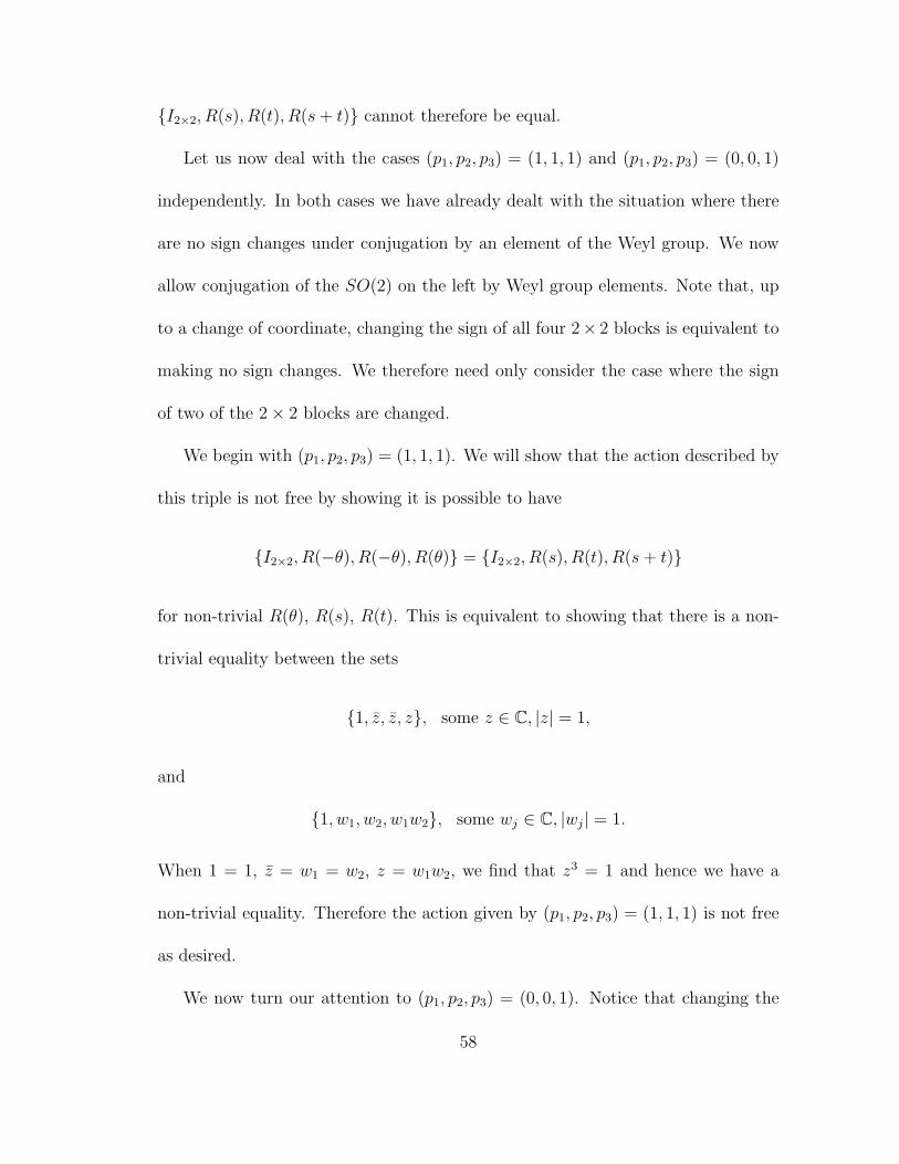
I2×2, R(s), R(t), R(s + t) cannot therefore be equal.

Let us now deal with the cases (p1, p2, p3) = (1, 1, 1) and (p1, p2, p3) = (0, 0, 1)

independently. In both cases we have already dealt with the situation where there

are no sign changes under conjugation by an element of the Weyl group. We now

allow conjugation of the SO(2) on the left by Weyl group elements. Note that, up

to a change of coordinate, changing the sign of all four 2× 2 blocks is equivalent to

making no sign changes. We therefore need only consider the case where the sign

of two of the 2× 2 blocks are changed.

We begin with (p1, p2, p3) = (1, 1, 1). We will show that the action described by

this triple is not free by showing it is possible to have

I2×2, R(−θ), R(−θ), R(θ) = I2×2, R(s), R(t), R(s + t)

for non-trivial R(θ), R(s), R(t). This is equivalent to showing that there is a non-

trivial equality between the sets

1, z, z, z, some z ∈ C, |z| = 1,

and

1, w1, w2, w1w2, some wj ∈ C, |wj| = 1.

When 1 = 1, z = w1 = w2, z = w1w2, we find that z3 = 1 and hence we have a

non-trivial equality. Therefore the action given by (p1, p2, p3) = (1, 1, 1) is not free

as desired.

We now turn our attention to (p1, p2, p3) = (0, 0, 1). Notice that changing the

58

sign of two of the 2 × 2 blocks on the left leaves the three I2×2 blocks invariant.

Therefore it is clear that we will always have at least two of R(s), R(t) and R(s+ t)

equal to I2×2, which in turn implies R(θ) = R(s) = R(t) = I2×2. Hence the action

given by (p1, p2, p3) = (0, 0, 1) is free.

Note that there are many other free S1 × G2 actions on G. For example, a

similar analysis to above shows that we have a free S1 action on the left of G/G2

by matrices of the form

R(θ)

R(θ)

R(θ)

R(kθ)

(5.2.9)

where (k, 3) = 1.

However, only the action in Lemma 5.2.1 is isometric with respect to the K-

invariant metric 〈〈 , 〉〉 on G, and henceforth we will denote this action by U .

It follows immediately from the long exact homotopy sequence for fibrations that

a biquotient Spin(8)//(S1×G2) = S1\(S7×S7) must be simply connected. By the

lifting criterion for covering spaces the action by U on SO(8) described above lifts

to some action by S1×G2 on Spin(8). Therefore, together with Theorem 5.1.1, one

might expect that the resulting simply connected biquotient Spin(8)//(S1 ×G2) =

S1\(S7 × S7) is a non-trivial finite cover of SO(8)//(S1 × G2). In fact the lemma

below will demonstrate that this covering map is a diffeomorphism.

Lemma 5.2.2. M13 := SO(8)//(S1×G2) is simply connected and hence a quotient

of S7 × S7 by an S1 action.

59

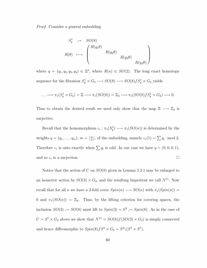
Proof. Consider a general embedding

S1q → SO(8)

R(θ) 7−→

R(q1θ)

R(q2θ)

R(q3θ)

R(q4θ)

where q = (q1, q2, q3, q4) ∈ Z4, where R(u) ∈ SO(2). The long exact homotopy

sequence for the fibration S1q ×G2 −→ SO(8) −→ SO(8)//S1

q ×G2 yields

. . . −→ π1(S1q ×G2) = Z −→ π1(SO(8)) = Z2 −→ π1(SO(8)//S1

q ×G2) −→ 0.

Thus to obtain the desired result we need only show that the map Z −→ Z2 is

surjective.

Recall that the homomorphism ι∗ : π1(S1q ) −→ π1(SO(n)) is determined by the

weights q = (q1, . . . , qm), m = bn2c, of the embedding, namely ι∗(1) =

∑qi mod 2.

Therefore ι∗ is onto exactly when∑

qi is odd. In our case we have q = (0, 0, 0, 1),

and so ι∗ is a surjection.

Notice that the action of U on SO(8) given in Lemma 5.2.1 may be enlarged to

an isometric action by SO(3)×G2, and the resulting biquotient we call N11. Now

recall that for all n we have a 2-fold cover Spin(n) −→ SO(n) with π1(Spin(n)) =

0 and π1(SO(n)) = Z2. Thus, by the lifting criterion for covering spaces, the

inclusion SO(3) → SO(8) must lift to Spin(3) = S3 → Spin(8). As in the case of

U = S1 ×G2 above we show that N11 = SO(8)//(SO(3)×G2) is simply connected

and hence diffeomorphic to Spin(8)//S3 ×G2 = S3\(S7 × S7).

60

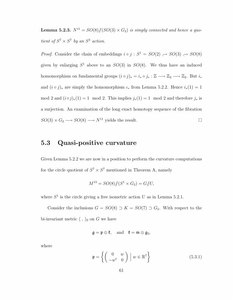
Lemma 5.2.3. N11 = SO(8)//(SO(3)×G2) is simply connected and hence a quo-

tient of S7 × S7 by an S3 action.

Proof. Consider the chain of embeddings i j : S1 = SO(2) → SO(3) → SO(8)

given by enlarging S1 above to an SO(3) in SO(8). We thus have an induced

homomorphism on fundamental groups (i j)∗ = i∗ j∗ : Z −→ Z2 −→ Z2. But i∗

and (i j)∗ are simply the homomorphism ι∗ from Lemma 5.2.2. Hence i∗(1) = 1

mod 2 and (i j)∗(1) = 1 mod 2. This implies j∗(1) = 1 mod 2 and therefore j∗ is

a surjection. An examination of the long exact homotopy sequence of the fibration

SO(3)×G2 −→ SO(8) −→ N11 yields the result.

5.3 Quasi-positive curvature

Given Lemma 5.2.2 we are now in a position to perform the curvature computations

for the circle quotient of S7 × S7 mentioned in Theorem A, namely

M13 = SO(8)//(S1 ×G2) = G//U,

where S1 is the circle giving a free isometric action U as in Lemma 5.2.1.

Consider the inclusions G = SO(8) ⊃ K = SO(7) ⊃ G2. With respect to the

bi-invariant metric 〈 , 〉0 on G we have

g = p⊕ k, and k = m⊕ g2,

where

p =

(0 w

−wt 0

) ∣∣∣ w ∈ R7

(5.3.1)

61

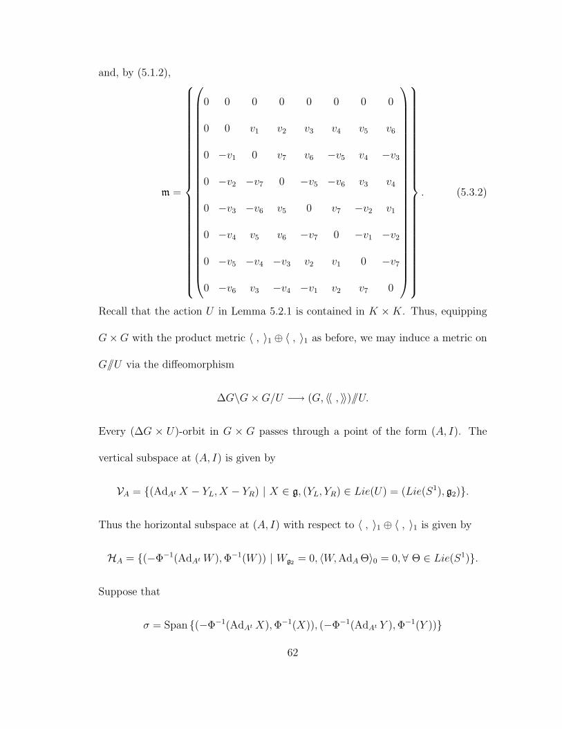
and, by (5.1.2),

m =

0 0 0 0 0 0 0 0

0 0 v1 v2 v3 v4 v5 v6

0 −v1 0 v7 v6 −v5 v4 −v3

0 −v2 −v7 0 −v5 −v6 v3 v4

0 −v3 −v6 v5 0 v7 −v2 v1

0 −v4 v5 v6 −v7 0 −v1 −v2

0 −v5 −v4 −v3 v2 v1 0 −v7

0 −v6 v3 −v4 −v1 v2 v7 0

. (5.3.2)

Recall that the action U in Lemma 5.2.1 is contained in K ×K. Thus, equipping

G×G with the product metric 〈 , 〉1 ⊕ 〈 , 〉1 as before, we may induce a metric on

G//U via the diffeomorphism

∆G\G×G/U −→ (G, 〈〈 , 〉〉)//U.

Every (∆G × U)-orbit in G × G passes through a point of the form (A, I). The

vertical subspace at (A, I) is given by

VA = (AdAt X − YL, X − YR) | X ∈ g, (YL, YR) ∈ Lie(U) = (Lie(S1), g2).

Thus the horizontal subspace at (A, I) with respect to 〈 , 〉1 ⊕ 〈 , 〉1 is given by

HA = (−Φ−1(AdAt W ), Φ−1(W )) | Wg2 = 0, 〈W, AdA Θ〉0 = 0, ∀ Θ ∈ Lie(S1).

Suppose that

σ = Span (−Φ−1(AdAt X), Φ−1(X)), (−Φ−1(AdAt Y ), Φ−1(Y ))

62

is a horizontal zero-curvature plane in g ⊕ g. Since we have equipped G × G with

the product metric 〈 , 〉1⊕〈 , 〉1, σ must project to zero-curvature planes σi, i = 1, 2,

on each factor.

Lemma 5.3.1. If σ = Span (−Φ−1(AdAt X), Φ−1(X)), (−Φ−1(AdAt Y ), Φ−1(Y ))

is a horizontal zero-curvature plane then it may be assumed without loss of generality

that X ∈ p and Y ∈ m.

Proof. σ2 has zero-curvature and hence X, Y must satisfy the conditions in (5.2.2).

[Xp, Yp] = 0 implies that, since (G,K) is a rank one symmetric pair, we may assume

Yp = 0 without loss of generality. Hence X ∈ p ⊕ m, Y ∈ m, since Xg2 = Yg2 = 0.

Now 0 = [Xk, Yk] if and only if 0 = [Xm, Ym]. But, by Theorem (i) and since the

bi-invariant metric on Spin(7) induces positive curvature on Spin(7)/G2 = S7,

there are no independent commuting vectors in m. Then, without loss of generality,

X ∈ p, Y ∈ m.

Thus we have

X =

(0 w

−wt 0

)∈ p, Y =

(0 0

0 (vij)

)∈ m,

and [X, Y ] = 0.

Now σ1 has zero curvature if and only if [(AdAt X)p, (AdAt Y )p] = 0, since

[AdAt X, AdAt Y ] = AdAt([X, Y ]) = 0.

Again, (G,K) is a rank one symmetric pair, thus σ1 has zero curvature if and only

if (AdAt X)p, (AdAt Y )p are linearly dependent. Since an element of p is determined

63

by its first row, for A = (aij) ∈ SO(8) we have

(AdAt X)p ∼8∑

k,`=1

ak1xk`a`j =8∑

`=2

(a11a`j − a`1a1j)w`, j = 2, . . . , 8, and

(AdAt Y )p ∼8∑

k,`=1

ak1yk`a`j =8∑

k,`=2

ak1vk`a`j, j = 2, . . . , 8.

If we assume that

A =

(R(θ)

I6×6

)∈ SO(8), θ 6= nπ

2, n ∈ Z,

then

(AdAt X)p ∼ (0, w2, w3 cos θ, w4 cos θ, w5 cos θ, w6 cos θ, w7 cos θ, w8 cos θ) and

(AdAt Y )p ∼ (0, 0, v1 sin θ, v2 sin θ, v3 sin θ, v4 sin θ, v5 sin θ, v6 sin θ).

Now (AdAt X)p, (AdAt Y )p are linearly dependent if and only if either (AdAt X)p = 0

or (AdAt Y )p = 0 or (AdAt X)p = s(AdAt Y )p, some s ∈ R− 0.

Suppose (AdAt X)p = 0. Then w2 = 0 and wj cos θ = 0, j = 3, . . . , 8. But

θ 6= nπ2

, hence wj = 0 for all j and so X = Xp = 0. Thus (AdAt X)p = 0 is

impossible.

Suppose now that (AdAt X)p = s(AdAt Y )p, some s ∈ R − 0. Then w2 = 0 and

wj = s vj−2 tan θ, 3 ≤ j ≤ 8. However, [X,Y ] = 0 implies that

8∑j=3

wjvj−2 = 0

and so we have a contradiction, as s 6= 0, θ 6= nπ2

.

64

Finally consider (AdAt Y )p = 0. θ 6= nπ2

implies that vj = 0, 1 ≤ j ≤ 6, and so

Y = Ym =

0

0

0 v7

−v7 0

0 v7

−v7 0

0 −v7

v7 0

.

Recall that 〈Y, AdA Θ〉0 = 0 for all Θ ∈ Lie(S1). But AdA Θ = Θ since A commutes

with S1. Hence we must have v7 = 0, i.e. Y = 0, and so (AdAt Y )p = 0 is impossible.

We have shown that there are no horizontal zero-curvature planes at (A, I),

and therefore have proved that the image of (A, I) in G//U is a point of positive

curvature. We have proved the curvature part of Theorem A(v):

Theorem 5.3.2. The manifold M13 = SO(8)//(S1 × G2) = G//U admits a metric

with quasi-positive curvature.

Since extending the U action to an action by SO(3)×G2 increases the number

of conditions which must be satisfied in order for a zero-curvature plane to be

horizontal, Theorem A(vi) follows immediately:

Corollary 5.3.3. The manifold N11 = SO(8)//(SO(3)×G2) admits a metric with

quasi-positive curvature.

65

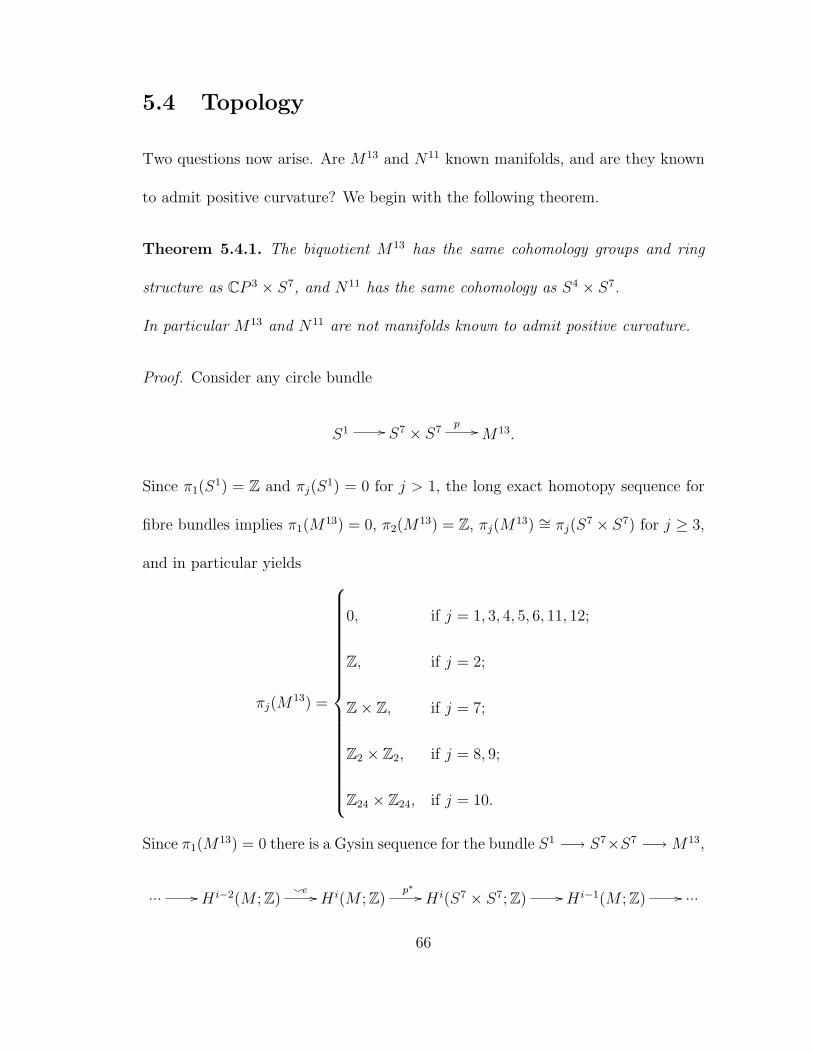
5.4 Topology

Two questions now arise. Are M13 and N11 known manifolds, and are they known

to admit positive curvature? We begin with the following theorem.

Theorem 5.4.1. The biquotient M13 has the same cohomology groups and ring

structure as CP 3 × S7, and N11 has the same cohomology as S4 × S7.

In particular M13 and N11 are not manifolds known to admit positive curvature.

Proof. Consider any circle bundle

S1 // S7 × S7p // M13.

Since π1(S1) = Z and πj(S

1) = 0 for j > 1, the long exact homotopy sequence for

fibre bundles implies π1(M13) = 0, π2(M

13) = Z, πj(M13) ∼= πj(S

7 × S7) for j ≥ 3,

and in particular yields

πj(M13) =

0, if j = 1, 3, 4, 5, 6, 11, 12;

Z, if j = 2;

Z× Z, if j = 7;

Z2 × Z2, if j = 8, 9;

Z24 × Z24, if j = 10.

Since π1(M13) = 0 there is a Gysin sequence for the bundle S1 −→ S7×S7 −→ M13,

... // H i−2(M ;Z)`e // H i(M ;Z)

p∗ // H i(S7 × S7;Z) // H i−1(M ;Z) // ...

66

Recall that

Hj(S7 × S7;Z) =

Z, if j = 0, 14;

Z⊕ Z, if j = 7;

0, otherwise.

Since we have a circle bundle S1 −→ S7 × S7 −→ M13, there is an isomorphism

H0(M ;Z) ∼= H0(S7 × S7) = Z, and the Euler class e ∈ H2(M ;Z).

The Gysin sequence gives groups Hj(M ;Z) = Z, j = 0, 2, 4, 6, and Hj(M ;Z) =

0, j = 1, 3, 5. By Poincare Duality and the Universal Coefficient Theorem we thus

have

Hj(M13;Z) =

Z, if j = 0, 2, 4, 6, 7, 9, 11, 13;

0, if j = 1, 3, 5, 8, 10, 12.

Hence, looking at the Serre spectral sequence for a fibration S1 −→ S7 × S7 −→

M13, we see that M13 has cohomology ring H∗(M ;Z) = Z[α, β]/〈α4, β2〉, where

α ∈ H2(M) and β ∈ H7(M). Therefore M13 has the same cohomology as CP 3×S7.

The analogous Gysin sequence computation for S3 −→ S7 × S7 −→ N11 yields

Hj(N11;Z) =

Z, if j = 0, 4, 7, 11;

0, if j = 1, 2, 3, 5, 6, 8, 9, 10,

and the Euler class e ∈ H4(N11;Z). Looking at the Serre spectral sequence for a

fibration S3 −→ S7 × S7 −→ N11 we find that N11 has cohomology ring structure

H∗(N11;Z) = Z[α, β]/〈α2, β2〉, , where α ∈ H4(N11) and β ∈ H7(N11), and so N11

has the same cohomology as S4 × S7.

67

Before we continue we prove an easy lemma which will prove useful in the

topological computations to follow.

Lemma 5.4.2. Consider a triple (r1, r2, r3) such that∑

ri = 0. Let σi(r) and

σi(r2) denote the ith elementary symmetric polynomials in r1, r2, r3 and r2

1, r22, r

23

respectively. Then σ1(r2) = −2σ2(r) and σ2(r

2) = σ2(r)2.

Proof. Since σ1(r) =∑

ri = 0 we have

0 = σ1(r)2

= (r21 + r2

2 + r23) + 2(r1r2 + r1r3 + r2r3)

= σ1(r2) + 2σ2(r)

as desired. On the other hand

σ2(r)2 − σ2(r

2) = (r1r2 + r1r3 + r2r3)2 − (r2

1r22 + r2

1r23 + r2

2r23)

= 2(r21r2r3 + r1r

22r3 + r1r2r

23)

= 2r1r2r3(r1 + r2 + r3)

= 0.

In [E1] (pages vii and 139), Eschenburg provides a beautiful diagram which

explicitly describes the embedding of the root system G2 into B3. Recall that B3 is

the root system corresponding to the Lie algebra so(7) and is given by

B3 = ±ti | 1 ≤ i ≤ 3 ∪ ±(ti ± tj) | 1 ≤ i < j ≤ 3.

68

The root system G2 lies on a hypersurface in Span B3 and is given by

G2 = ±si | 1 ≤ i ≤ 3 ∪ ±(si − sj) | 1 ≤ i < j ≤ 3,

where si = 13(2ti − tj − tk), i, j, k = 1, 2, 3. Notice that

∑si = 0 and that

si−sj = ti−tj ∈ B3. Furthermore, si is the projection of ti ∈ B3 and −(tj+tk) ∈ B3

onto the hypersurface containing G2.

Since the Lie group G2 is simply connected and has no centre, we see that the

inclusions

exp−1(I) = integral lattice of G2 ⊂ root lattice of G2 ⊂ weight lattice of G2

are in fact equalities. Therefore, by our above discussion of the roots of G2, the

integral and weight lattices of G2 are spanned by si | 1 ≤ i ≤ 3, ∑si = 0. Thus

by an abuse of notation we may assume that si | 1 ≤ i ≤ 3, ∑si = 0, spans

H1(TG2 ;Z) = Hom(Γ,Z), where TG2 is a maximal torus of G2 and Γ is the integral

lattice of G2.

Recall that Lemma 5.2.2 showed that

M13 := SO(8)//(S1 ×G2)

is a quotient of S7 × S7 by a particular S1 action.

Theorem 5.4.3. The first Pontrjagin class of M13 is

p1(M13) = 2α2

where α is a generator of H2(M13;Zp) = Zp, p prime, p ≥ 3.

69

Before we provide the proof we remark that, in terms of integral cohomology,

the theorem tells us only that p1(M13) is not divisible by any primes p ≥ 3. Thus

p1(M13) = ±2k ∈ Z = H4(M13), for some k ∈ Z, k ≥ 0. Since p(M × N) =

p(M) ⊗ p(N), p(Sn) = 1, and p(CP n) = (1 + β2)n+1, where β is the generator of

H2(CP n;Z), we find that p1(CP 3 × S7) = 4(β ⊗ 1)2. Therefore we are unable to

distinguish M13 and CP 3 × S7 using the theorem.

Proof of Theorem 5.4.3. We follow the techniques developed in [BH], [E2] and

[Si] (see also [FZ1]). Our strategy is to compute the first Pontrjagin class of the

quotient M13 using the descriptions given in Lemma 5.2.2 as biquotients of SO(8)

by S1 ×G2.

Let G = SO(8). Define the inclusions

fq : H := S1q → G

R(u) 7−→

R(q1u)

R(q2u)

R(q3u)

R(q4u)

where q = (q1, q2, q3, q4) ∈ Z4, and

g : K := G2 → G

given by the embedding of G2 into SO(7) ⊂ SO(8). For a general Lie group L, let

EL denote a contractible space on which L acts freely, and denote the classifying

space EL/L by BL. For the sake of notation we denote a product of Lie groups

L1 × L2 by L1L2.

70

Consider the following commutative diagram of fibrations

G× EGG//

²²

G× EGG

²²G×HK EGG

ϕG //

(ϕH ,ϕK)²²

G×GG EGG

B∆

²²

= B∆G

BH ×BK(Bfq ,Bg)

// BG ×BG

(5.4.1)

where ϕG, ϕK , and ϕH are the respective classifying maps, and ∆ : G −→ GG

denotes the diagonal embedding. Now, since projection onto the first factor in each

case is a homotopy equivalence, we have G ' G×EGG and H\G/K ' G×HK EGG.

Thus, up to homotopy, we can consider the diagram as

G //

²²

G

²²H\G/K //

²²

B∆G

B∆

²²BH ×BK

(Bfq ,Bg)// BG ×BG

Recall that SO(8) and G2 have torsion in their cohomology for coefficients in Z and

Z2 (see [MT]). Therefore, using Zp coefficients with p ≥ 3 and prime, we have

H∗(G;Zp) = Λ(y1, y2, y3, y4), y1 ∈ H3, y2, y4 ∈ H7, y3 ∈ H11,

H∗(K;Zp) = Λ(x1, x2), x1 ∈ H3, x2 ∈ H11,

H∗(H;Zp) = Λ(u), u ∈ H1.

71

Hence

H∗(BG;Zp) = Zp[y1, y2, y3, y4], y1 ∈ H4, y2, y4 ∈ H8, y3 ∈ H12

H∗(BK ;Zp) = Zp[x1, x2], x1 ∈ H4, x2 ∈ H12

H∗(BH ;Zp) = Zp[u], u ∈ H2,

where yi, xj and u denote the transgressions of yi, xj and u respectively.

Let TG and TK be the maximal tori of G and K, with coordinates (t1, t2, t3, t4)

and (s1, s2, s3),∑

si = 0, respectively. By an abuse of notation we will identify

ti and sj with the elements ti ∈ H1(TG) and sj ∈ H1(TK). Hence ti ∈ H2(BTG),

sj ∈ H2(BTK). Since G and K do not have any torsion in their cohomologies we

have

H∗(BG) = H∗(BTG)WG = Zp[t1, . . . , t4]

WG and

H∗(BK) = H∗(BTK)WK = Zp[s1, s2, s3]

WK

where WL denotes the Weyl group of L.

WG acts on H∗(BTG) via permutations in ti and an even number of sign changes.

Therefore a basis for H∗(BTG)WG is given by elementary symmetric polynomials

σi(t2) := σi(t

21, . . . , t

24), i = 1, 2, 3, and t1t2t3t4. Hence we choose yi = σi(t

2),

i = 1, 2, 3, and y4 = t1t2t3t4.

WG2 = WK is the dihedral group of order twelve. Its action on the root system

G2 is by rotations of π3

and by reflections through the horizontal axis. Therefore,

given our description of the root system of G2 above, WK acts on H∗(BTK) via per-

72

mutations in si and a simultaneous sign change of all si. Thus we see that elements

of H∗(BTK) which are invariant under WK are given by sums and products of the

elementary symmetric polynomials σ2(s) := σ2(s1, s2, s3) and σi(s2) := σi(s

21, s

22, s

23),

i = 1, 2, 3. However, since∑

si = 0, Lemma 5.4.2 shows that a basis for H∗(BTK)WK

is given by the symmetric polynomials σi(s2), i = 1, 3. Thus we identify x1 = σ1(s

2)

and x2 = σ3(s2).

Therefore we have

H∗(BG;Zp) = Zp[σ1(t2), σ2(t

2), σ3(t2), t1t2t3t4], (5.4.2)

H∗(BK ;Zp) = Zp[σ1(s2), σ3(s

2)]. (5.4.3)

Let h : L1 −→ L2 be a homomorphism of Lie groups. Then the commutative

diagram

L1h // L2

TL1

?Â

OO

h// TL2

?Â

OO

induces a commutative diagram

BL1

Bh // BL2

BTL1

OO

Bh

// BTL2

OO(5.4.4)

which in turn induces the commutative diagram

H∗(BL1)

²²

H∗(BL2)(Bh)∗oo

²²H∗(BTL1

) H∗(BTL2)

(Bh)∗oo

(5.4.5)

73

Recall that

H∗(BGG) = H∗(BG)⊗H∗(BG) = H∗(BTG)WG ⊗H∗(BTG

)WG

= Zp[t1, . . . , t4]WG ⊗ Zp[t1, . . . , t4]

WG

= Zp[y1, y2, y3, y4]⊗ Zp[y1, y2, y3, y4],

where Zp[y1, y2, y3, y4] = Zp[σ1(t2), σ2(t

2), σ3(t2), t1t2t3t4] as before. Consider the

diagonal embedding ∆ : G → GG. In coordinates ∆|TGis given by ti 7−→ (ti, ti),

i = 1, . . . , 4. We have commutative diagrams as in (5.4.4) and (5.4.5). Now

∆∗ : H1(TG)⊗H1(TG) −→ H1(TG)

ti ⊗ 1 7−→ ti

1⊗ ti 7−→ ti,

which in turn implies

(B∆)∗ : H2(BTG)⊗H2(BTG

) −→ H2(BTG)

ti ⊗ 1 7−→ ti

1⊗ ti 7−→ ti.

Therefore,

(B∆)∗ : H∗(BGG) −→ H∗(BG)

yi ⊗ 1 7−→ yi

1⊗ yi 7−→ yi.

74

Since the diagram (5.4.1) is commutative we see that

ϕ∗G(yi) = ϕ∗G((B∆)∗(yi ⊗ 1)) = ϕ∗H((Bfq)∗(yi)), and

ϕ∗G(yi) = ϕ∗G((B∆)∗(1⊗ yi)) = ϕ∗K((Bg)∗(yi)).

Consider now fq : H := S1q → G as above. In coordinates fq is given by

u 7−→ (q1u, . . . , q4u).

We get commutative diagrams as in (5.4.4) and (5.4.5). Now

(fq)∗ : H1(TG) −→ H1(S1

q )

ti 7−→ qiu,

which implies that

(Bfq)∗ : H2(BTG

) −→ H2(BS1q)

ti 7−→ qiu.

Therefore, letting q2 := (q21, . . . , q

24), we have

(Bfq)∗ : H∗(BG) −→ H∗(BS1

q)

yi 7−→ σi(q2)u2i, i = 1, 2, 3, (5.4.6)

y4 7−→ σ4(q)u4.

On the other hand, now consider g : K := G2 → G ⊂ SO(8) as above. In particular,

g|TK: TK −→ TG, and examining TK as in (5.1.3) we see that in coordinates g|TK

75

is given by (s1, s2, s3) 7−→ (0, s1, s2,−s3),∑

si = 0. Again we get commutative

diagrams as in (5.4.4) and (5.4.5). Now

(g|TK)∗ : H1(TG) −→ H1(TK)

t1 7−→ 0,

ti 7−→ si−1, i = 2, 3,

t4 7−→ −s3

and hence

(Bg|TK)∗ : H2(BTG

) −→ H2(BTK)

t1 7−→ 0,

ti 7−→ si−1, i = 2, 3,

t4 7−→ −s3

Therefore we have

(Bg)∗ : H∗(BG) −→ H∗(BK)

y1 7−→ σ1(s2) = x1, (5.4.7)

y2 7−→ σ2(s2),

y3 7−→ σ3(s2) = x2,

y4 7−→ 0.

Thus (Bg)∗(y1) = x1 and (Bg)

∗(y3) = x2.

76

We are now in a position to compute the Pontrjagin class of H\G/K, and in

particular p1. Let τ be the tangent bundle of H\G/K. In [Si] the following vector

bundles over H\G/K were introduced. Let αH := (G/K) ×H h, where H acts on

G/K on the left, and on h via AdH . Let αK := (H\G)×K k, where K acts on H\G

on the right, and on k via AdK . Finally, let αG := ((H\G)× (G/K))×G g, where G

acts on (H\G) × (G/K) via (Hg1, g2K) ? g = (Hg1g, g−1g2K), and on g via AdG.

Since H ×K acts freely on G we have

τ ⊕ αH ⊕ αK = αG.

Recall from [BH] that the Pontrjagin class of a homogeneous vector bundle αL =

P ×L V associated to the L-principal bundle P −→ B := P/L is given by

p(αL) = 1 + p1(αL) + p2(αL) + · · · = ϕ∗L(a), a :=∏

αi∈∆+L

(1 + α2i ),

where ∆+L is the set of positive weights of the representation of L on V , and ϕL :

B −→ BL is the classifying map of the L-principal bundle. We have identified

αi ∈ H1(TL) ∼= H2(BTL), and hence a ∈ H∗(BTL

)WL ∼= H∗(BL)

In our case the vector bundles αH , αK , αG are associated to a principal bundle

and the weights are the roots of the corresponding Lie group.

Since H = S1 we have p(αH) = 1, and since, if V , W are vector bundles over

some manifold M , p(V ⊕W ) = p(V ) ` p(W ), we have

p(τ)p(αK) = p(αG).

77

By our discussion above and since inverses are well-defined in the polynomial algebra

H∗(BK) it follows that

p(τ) = ϕ∗G(a)ϕ∗K(b−1),

where a :=∏

αi∈∆+G(1 + α2

i ) and b :=∏

βj∈∆+K(1 + β2

j ). In particular, note that

p1(τ) = p1(αG)− p1(αK)

= ϕ∗G

∑

αi∈∆+G

α2i

− ϕ∗K

∑

βj∈∆+K

β2j

.

The positive roots of G = SO(8) are ti ± tj, 1 ≤ i < j ≤ 4. Hence

∑

αi∈∆+G

α2i =

∑1≤i<j≤4

((ti − tj)

2 + (ti + tj)2)

= 2∑

1≤i<j≤4

(t2i + t2j)

= 64∑

i=1

t2i

= 6y1.

Now ϕ∗G(y1) = ϕ∗H((Bfq)∗(y1)) = σ1(q

2)ϕ∗H(u2). Hence p1(αG) = 6σ1(q2)ϕ∗H(u2) ∈

H4(H\G/K).

From our earlier description of the roots of G2, the positive roots of K = G2 are

s1, s2, −s3, s1 − s3, s2 − s1, s2 − s3,

78

where∑

si = 0. Then

∑

βj∈∆+K

β2j = s2

1 + s22 + s2

3 + (s1 − s3)2 + (s2 − s1)

2 + (s2 − s3)2

= σ1(s2) + (s2

1 + s23 − 2s1s3) + (s2

1 + s22 − 2s1s2) + (s2

2 + s23 − 2s2s3)

= 3σ1(s2)− 2σ2(s)

= 4σ1(s2) by Lemma 5.4.2

= 4x1

Thus, since

ϕ∗K(x1) = ϕ∗K((Bg)∗(y1)) = ϕ∗H((Bfq)

∗(y1)) = σ1(q2)ϕ∗H(u2),

we have p1(αK) = 4σ1(q2)ϕ∗H(u2) ∈ H4(H\G/K). Hence

p1(τ) = p1(αG)− p1(αK)

= 2σ1(q2)ϕ∗H(u2) ∈ H4(H\G/K)

In our case we have q = (0, 0, 0, 1). Therefore p1(M13) = p1(τ) = 2ϕ∗H(u2).

Consider the Serre spectral sequence for the fibration G −→ H\G/K −→ BHK .

Notice that u ∈ H2(BH) = H2(BHK) = E2,02 will survive until E∞ since H∗(G)

contains no elements of degree 1. Recall that the classifying map ϕ∗H is the edge

homomorphism

ϕ∗H : H i(BHK) = Ei,02 ³ Ei,0

∞ → H i(H\G/K).

Therefore, given Theorem 5.4.1, ϕ∗H(u) is mapped to a non-zero element, i.e. a

generator, of H2(H\G/K;Zp) = Zp and hence ϕ∗H(u2) 6= 0.

79

Whilst we are as yet unable to distinguish M13 and CP 3 × S7, we have more

luck when we consider N11.

Theorem 5.4.4. The manifold N11 = SO(8)//(SO(3) × G2) has first Pontrjagin

class

p1(N11) = α,

where α is a generator of H4(N11;Zp) = Zp, p prime, p ≥ 3.

Proof. We let G and K be as above, H = SO(3), and retain the notation and

techniques used in the proof of Theorem 5.4.3.

Again using Zp coefficients with p ≥ 3 and prime, we have

H∗(G;Zp) = Λ(y1, y2, y3, y4), y1 ∈ H3, y2, y4 ∈ H7, y3 ∈ H11,

H∗(K;Zp) = Λ(x1, x2), x1 ∈ H3, x2 ∈ H11,

H∗(H;Zp) = Λ(w), w ∈ H3.

Hence

H∗(BG;Zp) = Zp[y1, y2, y3, y4], y1 ∈ H4, y2, y4 ∈ H8, y3 ∈ H12

H∗(BK ;Zp) = Zp[x1, x2], x1 ∈ H4, x2 ∈ H12

H∗(BH ;Zp) = Zp[w], w ∈ H2,

where yi, xj and w denote the transgressions of yi, xj and w respectively.

Let TH be the maximal tori of H with coordinate u. By an abuse of notation

we will identify u with the element u ∈ H1(TH). Hence u ∈ H2(BTH). Since G, K

80

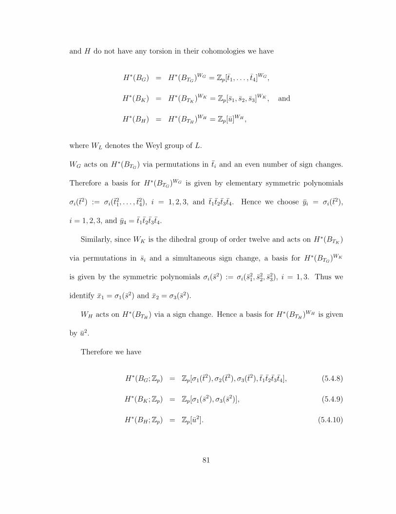
and H do not have any torsion in their cohomologies we have

H∗(BG) = H∗(BTG)WG = Zp[t1, . . . , t4]

WG ,

H∗(BK) = H∗(BTK)WK = Zp[s1, s2, s3]

WK , and

H∗(BH) = H∗(BTH)WH = Zp[u]WH ,

where WL denotes the Weyl group of L.

WG acts on H∗(BTG) via permutations in ti and an even number of sign changes.

Therefore a basis for H∗(BTG)WG is given by elementary symmetric polynomials

σi(t2) := σi(t

21, . . . , t

24), i = 1, 2, 3, and t1t2t3t4. Hence we choose yi = σi(t

2),

i = 1, 2, 3, and y4 = t1t2t3t4.

Similarly, since WK is the dihedral group of order twelve and acts on H∗(BTK)

via permutations in si and a simultaneous sign change, a basis for H∗(BTG)WK

is given by the symmetric polynomials σi(s2) := σi(s

21, s

22, s

23), i = 1, 3. Thus we

identify x1 = σ1(s2) and x2 = σ3(s

2).

WH acts on H∗(BTH) via a sign change. Hence a basis for H∗(BTH

)WH is given

by u2.

Therefore we have

H∗(BG;Zp) = Zp[σ1(t2), σ2(t

2), σ3(t2), t1t2t3t4], (5.4.8)

H∗(BK ;Zp) = Zp[σ1(s2), σ3(s

2)], (5.4.9)

H∗(BH ;Zp) = Zp[u2]. (5.4.10)

81

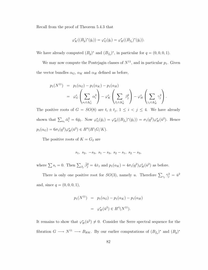
Recall from the proof of Theorem 5.4.3 that

ϕ∗K((Bg)∗(yi)) = ϕ∗G(yi) = ϕ∗H((Bfq)

∗(yi)).

We have already computed (Bg)∗ and (Bfq)

∗, in particular for q = (0, 0, 0, 1).

We may now compute the Pontrjagin classes of N11, and in particular p1. Given

the vector bundles αG, αK and αH defined as before,

p1(N11) = p1(αG)− p1(αK)− p1(αH)

= ϕ∗G

∑

αi∈∆+G

α2i

− ϕ∗K

∑

βj∈∆+K

β2j

− ϕ∗H

∑

γj∈∆+H

γ2j

.

The positive roots of G = SO(8) are ti ± tj, 1 ≤ i < j ≤ 4. We have already

shown that∑

αiα2

i = 6y1. Now ϕ∗G(y1) = ϕ∗H((Bfq)∗(y1)) = σ1(q

2)ϕ∗H(u2). Hence

p1(αG) = 6σ1(q2)ϕ∗H(u2) ∈ H4(H\G/K).

The positive roots of K = G2 are

s1, s2, −s3, s1 − s3, s2 − s1, s2 − s3,

where∑

si = 0. Then∑

βjβ2

j = 4x1 and p1(αK) = 4σ1(q2)ϕ∗H(u2) as before.

There is only one positive root for SO(3), namely u. Therefore∑

γjγ2

j = u2

and, since q = (0, 0, 0, 1),

p1(N11) = p1(αG)− p1(αK)− p1(αH)

= ϕ∗H(u2) ∈ H4(N11).

It remains to show that ϕ∗H(u2) 6= 0. Consider the Serre spectral sequence for the

fibration G −→ N11 −→ BHK . By our earlier computations of (Bfq)∗ and (Bg)

∗

82

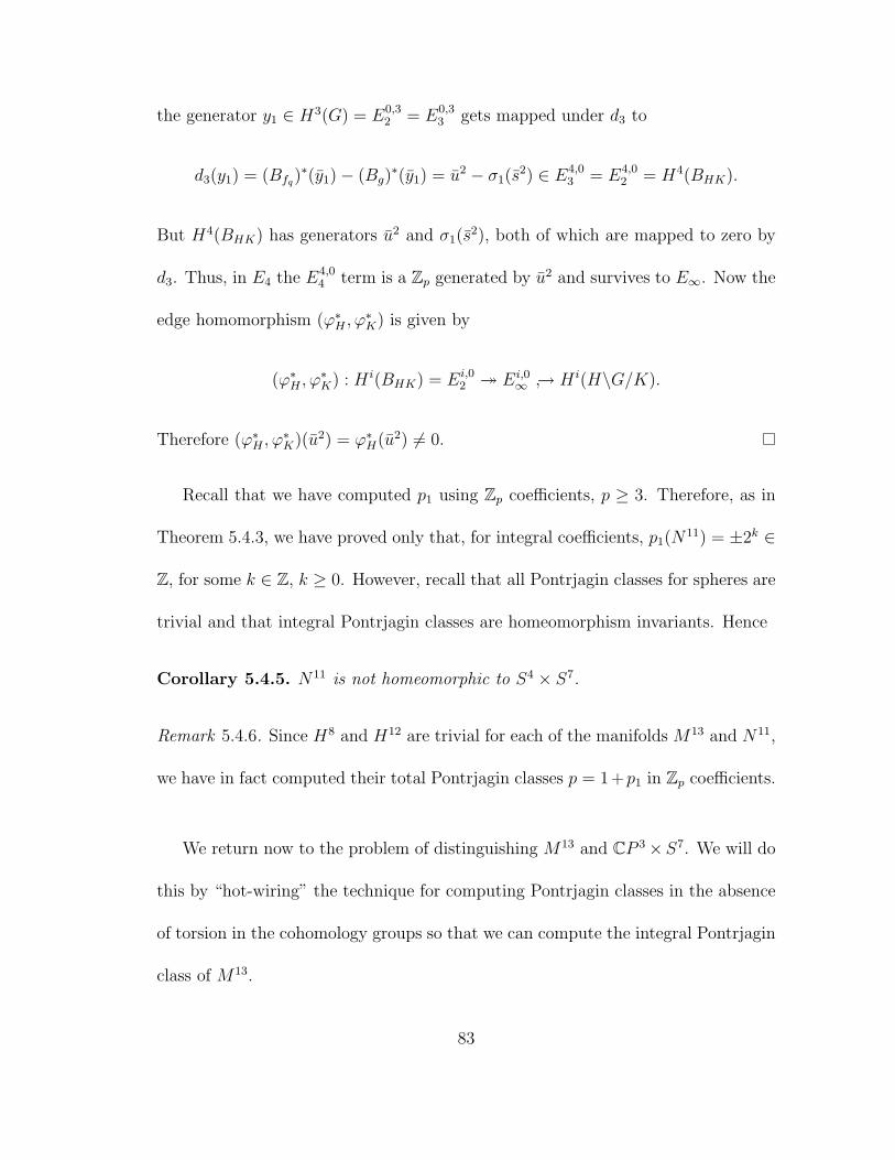
the generator y1 ∈ H3(G) = E0,32 = E0,3

3 gets mapped under d3 to

d3(y1) = (Bfq)∗(y1)− (Bg)

∗(y1) = u2 − σ1(s2) ∈ E4,0

3 = E4,02 = H4(BHK).

But H4(BHK) has generators u2 and σ1(s2), both of which are mapped to zero by

d3. Thus, in E4 the E4,04 term is a Zp generated by u2 and survives to E∞. Now the

edge homomorphism (ϕ∗H , ϕ∗K) is given by

(ϕ∗H , ϕ∗K) : H i(BHK) = Ei,02 ³ Ei,0

∞ → H i(H\G/K).

Therefore (ϕ∗H , ϕ∗K)(u2) = ϕ∗H(u2) 6= 0.

Recall that we have computed p1 using Zp coefficients, p ≥ 3. Therefore, as in

Theorem 5.4.3, we have proved only that, for integral coefficients, p1(N11) = ±2k ∈

Z, for some k ∈ Z, k ≥ 0. However, recall that all Pontrjagin classes for spheres are

trivial and that integral Pontrjagin classes are homeomorphism invariants. Hence

Corollary 5.4.5. N11 is not homeomorphic to S4 × S7.

Remark 5.4.6. Since H8 and H12 are trivial for each of the manifolds M13 and N11,

we have in fact computed their total Pontrjagin classes p = 1+p1 in Zp coefficients.

We return now to the problem of distinguishing M13 and CP 3×S7. We will do

this by “hot-wiring” the technique for computing Pontrjagin classes in the absence

of torsion in the cohomology groups so that we can compute the integral Pontrjagin

class of M13.

83

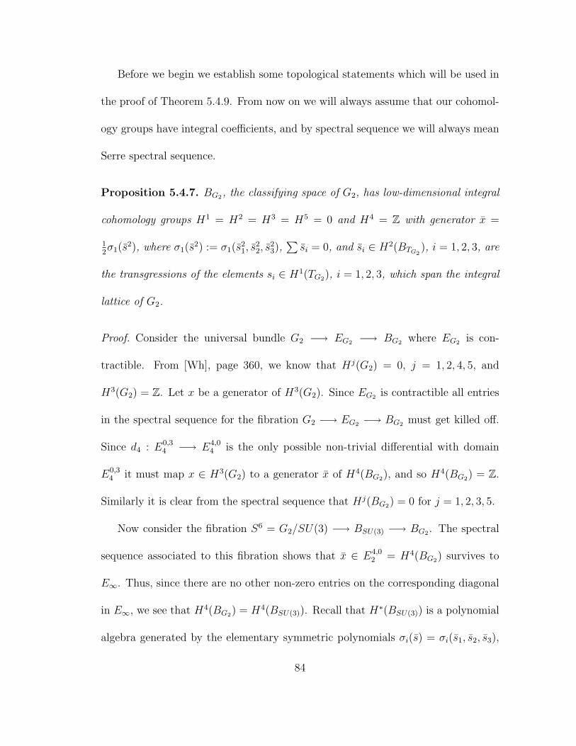
Before we begin we establish some topological statements which will be used in

the proof of Theorem 5.4.9. From now on we will always assume that our cohomol-

ogy groups have integral coefficients, and by spectral sequence we will always mean

Serre spectral sequence.

Proposition 5.4.7. BG2, the classifying space of G2, has low-dimensional integral

cohomology groups H1 = H2 = H3 = H5 = 0 and H4 = Z with generator x =

12σ1(s

2), where σ1(s2) := σ1(s

21, s

22, s

23),

∑si = 0, and si ∈ H2(BTG2

), i = 1, 2, 3, are

the transgressions of the elements si ∈ H1(TG2), i = 1, 2, 3, which span the integral

lattice of G2.

Proof. Consider the universal bundle G2 −→ EG2 −→ BG2 where EG2 is con-

tractible. From [Wh], page 360, we know that Hj(G2) = 0, j = 1, 2, 4, 5, and

H3(G2) = Z. Let x be a generator of H3(G2). Since EG2 is contractible all entries

in the spectral sequence for the fibration G2 −→ EG2 −→ BG2 must get killed off.

Since d4 : E0,34 −→ E4,0

4 is the only possible non-trivial differential with domain

E0,34 it must map x ∈ H3(G2) to a generator x of H4(BG2), and so H4(BG2) = Z.

Similarly it is clear from the spectral sequence that Hj(BG2) = 0 for j = 1, 2, 3, 5.

Now consider the fibration S6 = G2/SU(3) −→ BSU(3) −→ BG2 . The spectral

sequence associated to this fibration shows that x ∈ E4,02 = H4(BG2) survives to

E∞. Thus, since there are no other non-zero entries on the corresponding diagonal

in E∞, we see that H4(BG2) = H4(BSU(3)). Recall that H∗(BSU(3)) is a polynomial

algebra generated by the elementary symmetric polynomials σi(s) = σi(s1, s2, s3),

84

i = 2, 3, in the transgressions sj of sj ∈ H1(TSU(3)), j = 1, 2, 3, where the sj span

the integral lattice of SU(3). Note that∑

sj = 0, TG2 = TSU(3) and deg(σi(s)) = 2i.

Therefore H4(BG2) is generated by σ2(s). However, by Lemma 5.4.2 we see that

σ2(s) = −12σ1(s

2). We set x = 12σ1(s

2).

Proposition 5.4.8. The manifold SO(8)/G2 = (S7 × S7)/Z2 has low-dimensional

integral cohomology groups Hj(SO(8)/G2) = Hj(RP 7), 0 ≤ j ≤ 6.

Proof. Consider the spectral sequence for the fibration

RP 7 = SO(7)/G2 −→ SO(8)/G2 −→ SO(8)/SO(7) = S7.

Recall that

Hj(RP 7) =

Z if j = 0, 7

Z2 if j = 2, 4, 6

0 if j = 1, 3, 5.

It is clear that each E0,j2 = Hj(RP 7), j ≤ 5, survives to E∞. For E0,6

2 = H6(RP 7) =

Z2 notice that there are no non-trivial homomorphisms Z2 −→ Z and so the dif-

ferential d7 : E0,67 = Z2 −→ E7,0

7 = Z must be trivial. Therefore E0,62 = H6(RP 7)

also survives to E∞. Since there are no other non-zero entries on the corresponding

diagonals we get the desired result.

We are now in a position to complete the proof of Theorem A(v).

85

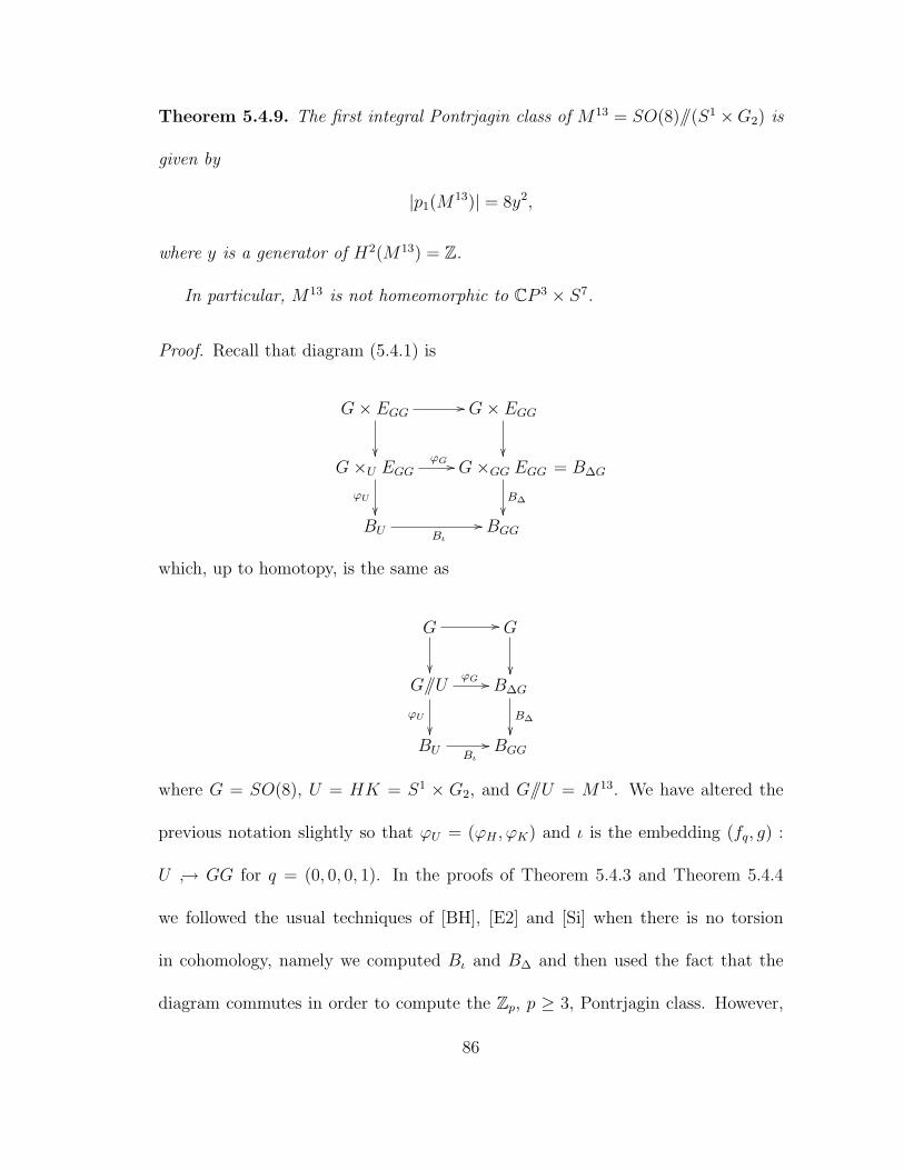
Theorem 5.4.9. The first integral Pontrjagin class of M13 = SO(8)//(S1 ×G2) is

given by

|p1(M13)| = 8y2,

where y is a generator of H2(M13) = Z.

In particular, M13 is not homeomorphic to CP 3 × S7.

Proof. Recall that diagram (5.4.1) is

G× EGG//

²²

G× EGG

²²G×U EGG

ϕG //

ϕU

²²

G×GG EGG

B∆

²²

= B∆G

BU Bι

// BGG

which, up to homotopy, is the same as

G //

²²

G

²²G//U

ϕG //

ϕU

²²

B∆G

B∆

²²BU Bι

// BGG

where G = SO(8), U = HK = S1 × G2, and G//U = M13. We have altered the

previous notation slightly so that ϕU = (ϕH , ϕK) and ι is the embedding (fq, g) :

U → GG for q = (0, 0, 0, 1). In the proofs of Theorem 5.4.3 and Theorem 5.4.4

we followed the usual techniques of [BH], [E2] and [Si] when there is no torsion

in cohomology, namely we computed Bι and B∆ and then used the fact that the

diagram commutes in order to compute the Zp, p ≥ 3, Pontrjagin class. However,

86

since SO(8) and G2 have torsion in integral cohomology, we need to adopt a different

approach in order to compute the integral Pontrjagin class. Since H8(M13) =

H12(M13) = 0 we can restrict our attention to the first integral Pontrjagin class

p1(M13) ∈ H4(M13). The key idea to be taken from the proofs of Theorem 5.4.3

and Theorem 5.4.4 is that we computed the first Pontrjagin classes of some vector

bundles over B∆G and BU , then pulled them back to M13 under the classifying maps

ϕG and ϕU respectively. As it turns out, the first Pontrjagin classes of the vector

bundles over B∆G and BU are the same in integral coefficients as in Zp coefficients,

p ≥ 3. Our strategy, therefore, is to compute the maps ϕ∗U : H4(BU) −→ H4(M13)

and ϕ∗G : H4(B∆G) −→ H4(M13) and pull back the respective first Pontrjagin

classes.

As a first step in computing ϕ∗U : H4(BU) −→ H4(M13) we notice that H∗(U) =

H∗(S1) ⊗ H∗(G2) and H∗(BU) = H∗(BS1) ⊗ H∗(BG2) since H∗(S1) and H∗(BS1)

are torsion-free. Therefore

Hj(U) =

Z if j = 0

Z = 〈w〉 if j = 1

Z = 〈x〉 if j = 3

0 if j = 2, 4, 5

where w is a generator of H1(S1) and x is a generator of H3(G2), and applying

87

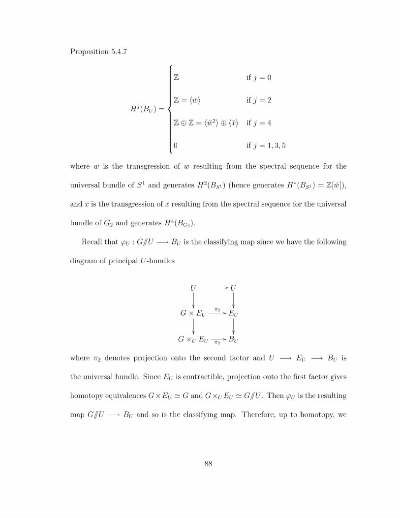
Proposition 5.4.7

Hj(BU) =

Z if j = 0

Z = 〈w〉 if j = 2

Z⊕ Z = 〈w2〉 ⊕ 〈x〉 if j = 4

0 if j = 1, 3, 5

where w is the transgression of w resulting from the spectral sequence for the

universal bundle of S1 and generates H2(BS1) (hence generates H∗(BS1) = Z[w]),

and x is the transgression of x resulting from the spectral sequence for the universal

bundle of G2 and generates H4(BG2).

Recall that ϕU : G//U −→ BU is the classifying map since we have the following

diagram of principal U -bundles

U //

²²

U

²²G× EU

π2 //

²²

EU

²²G×U EU π2

// BU

where π2 denotes projection onto the second factor and U −→ EU −→ BU is

the universal bundle. Since EU is contractible, projection onto the first factor gives

homotopy equivalences G×EU ' G and G×U EU ' G//U . Then ϕU is the resulting

map G//U −→ BU and so is the classifying map. Therefore, up to homotopy, we

88

may consider the following commutative diagram of fibrations

U //

²²

U

²²G //

²²

EU

²²G//U ϕU

// BU

Consider first the spectral sequence for the fibration on the left. Recall that

H∗(M13) = H∗(CP 3 × S7). Hence

Hj(G//U) =

Z if j = 0

Z = 〈y〉 if j = 2

Z = 〈y2〉 if j = 4

0 if j = 1, 3, 5.

Since G = SO(8) we have from [CMV] that

Hj(G) =

Z if j = 0

0 if j = 1

Z2 = 〈r〉 if j = 2

Z = 〈z〉 if j = 3

Z2 = 〈r2〉 if j = 4.

Since H1(G) = 0 we see that d2 : E0,12 = 〈w〉 −→ E2,0

2 = 〈y〉 must have trivial

kernel, i.e. d2(w) = ky for some k ∈ Z, k 6= 0. Then E0,23 = 〈y〉/〈ky〉 survives to

E∞ and since H2(G) = Z2 we must therefore have k = 2, i.e. d2(w) = 2y.

89

On the other hand, the spectral sequence shows that on the E4-page we have

the differential d4 : E0,34 = 〈x〉 −→ E0,4

4 = 〈y2〉/〈2y2〉. However, since H3(G) = Z

and H4(G) = Z2, we must have d4(x) = 0 ∈ 〈y2〉/〈2y2〉.

Since EU is contractible it is clear from the spectral sequence for the fibration

on the right that d2 : E0,12 = 〈w〉 −→ E2,0

2 = 〈w〉 is an isomorphism with d2(w) = w,

and d4 : E0,34 = 〈x〉 −→ E4,0

4 = 〈w2〉 ⊕ 〈x〉 is given by d4(x) = x.

By naturality of the spectral sequence we thus have for the left-hand fibration

that d2(w) = ϕ∗U(w) ∈ 〈y〉 and d4(x) = ϕ∗U(x) ∈ 〈y2〉/〈2y2〉. Therefore, since we

have already shown that d2(w) = 2y ∈ 〈y〉 and d4(x) = 0 ∈ 〈y2〉/〈2y2〉, we find

ϕ∗U(w) = 2y ∈ H2(G//U) = 〈y〉 and (5.4.11)

ϕ∗U(x) = 2ky2 ∈ H4(G//U) = 〈y2〉, for some k ∈ Z. (5.4.12)

We now turn our attention to computing ϕ∗G : H4(B∆G) −→ H4(M13). In order

to show that ϕG : G//U −→ B∆G is the classifying map consider the commutative

diagram of principal G-bundles

G //

²²

G

²²GG×U EGG

//

²²

GG×GG EGG

²²(∆G\GG)×U EGG ϕG

// (∆G\GG)×GG EGG

Since GG ×GG EGG = EGG and (∆G\GG) ×GG EGG = G ×GG EGG = B∆G we

see that the fibration on the right-hand side is the universal bundle for G. On the

left-hand side we have (∆G\GG)×U EGG = G×U EGG, and projection onto the first

90

factor gives homotopy equivalences GG×U EGG ' GG/U and G×U EGG ' G//U .

Thus up to homotopy the diagram becomes

G //

²²

G

²²GG/U //

²²

EGG

²²G//U ϕG

// BG

as desired. Recall that H3(G) = 〈z〉. The cohomology of BG is described in [Br]

and [F], but for our purposes we need only that

Hj(BG) =

Z if j = 0

0 if j = 1, 2

Z2 if j = 3

Z if j = 4

Z2 if j = 5.

Whilst proving Proposition 3.6 in [GZ2] the authors show that, since E = EGG is

contractible, in the spectral sequence for the bundle G −→ E −→ BG the differential

d4 : E0,34 = 〈2z〉 −→ E4,0

4 = H4(BG) is an isomorphism, i.e. 2z gets mapped to

a generator z of H4(BG) = Z. This follows from the facts that E2,22 = Z2 by the

Universal Coefficient Theorem, and that d2 : E0,32 = 〈z〉 −→ E2,2

2 = Z2 must be

onto.

Therefore naturality of the spectral sequence implies that d4(2z) = ϕ∗G(z) in

91

the spectral sequence for the left-hand fibration G −→ GG/U −→ G//U , where

H3(G) = 〈z〉 and H4(BG) = 〈z〉.

In order to determine the exact value of ϕ∗G(z) ∈ H4(G//U) we need to examine

the spectral sequence for the left-hand fibration. First we must compute the coho-

mology of GG/U in low-dimensions. Recall that GG/U = V8,6 × SO(8)/G2, where

V8,6 is the Stiefel manifold SO(8)/SO(2). From [CMV] we find that

Hj(V8,6) =

Z if j = 0, 2

0 if j = 1, 3, 5

Z2 if j = 4.

We computed the low-dimensional cohomology groups of SO(8)/G2 in Proposition

5.4.8. From the general Kunneth formula for cohomology ([Sp], page 247) we find

that

Hj(GG/U) =

Z if j = 0

0 if j = 1, 3

Z⊕ Z2 if j = 2

Z32 if j = 4

Z2 if j = 5.

Since H4(GG/U) = Z32, in the spectral sequence for G −→ GG/U −→ G//U the

differential d2 : E0,32 = H3(G) = 〈z〉 −→ E2,2

2 = Z2 must be trivial, i.e. E2,22 = Z2

must survive to E∞. It thus follows that Ei,j2 = Ei,j

3 = Ei,j4 for i ≤ 5, j ≤ 4.

92

Since H3(GG/U) = 0 the differential d4 : E0,34 = 〈z〉 −→ E4,0

4 = H4(G//U) = 〈y2〉

must be given by d4(z) = ny2 for some non-zero n ∈ Z. On the other hand, since

H4(GG/U) = Z32, E0,4

4 = E2,24 = Z2 and E1,3

4 = E3,14 = 0, the filtration for the

spectral sequence shows that n = 2, i.e. d4(z) = 2y2. But we have already shown

that d4(2z) = ϕ∗G(z). Therefore

ϕ∗G(z) = 4y2 ∈ H4(G//U) = 〈y2〉.

Furthermore, while proving Lemma 5.4 in [GZ2] the authors show that, by consid-

ering the spectral sequences of the fibrations SO(8)/SO(3) −→ BSO(3) −→ BSO(8)

and SO(3)/SO(2) −→ BSO(2) −→ BSO(3), we can let z = σ1(t2) = σ1(t

21, t

22, t

23, t

24),

where (t1, . . . , t4) are the coordinates of a maximal torus TG of G and by abuse of

notation we identify ti ∈ H1(TG) with ti ∈ H2(BTG) via transgression.

We are now in a position to compute the first Pontrjagin class of M13 = G//U .

Let τ be the tangent bundle of G//U . Consider the following vector bundles over

G//U . Let αU := G×U u, where U = S1 ×G2 acts on G via the biquotient action,

and on the Lie algebra u of U via AdU . Let αG := (GG/U)×G g, where G acts on

GG/U diagonally on the left and on g via AdG. Since U acts freely on G we have,

via a similar argument to that in [Si],

τ ⊕ αU = αG.

Recall that if V , W are vector bundles over some manifold M , p(V ⊕ W ) =

93

p(V ) ` p(W ). Hence in our case

p(τ)p(αU) = p(αG).

Recall from [BH] that, in the absence of torsion, the Pontrjagin class of a vector

bundle αL = P ×L V associated to the L-principal bundle P −→ B := P/L is given

by

p(αL) = 1 + p1(αL) + p2(αL) + · · · = ϕ∗L(a), a :=∏

αi∈∆+L

(1 + α2i ) ∈ H∗(BTL

)WL ,

where ∆+L is the set of positive weights of the representation of L on V , ϕL : B −→

BL is the classifying map of the L-principal bundle, and WL is the Weyl group of

L. Note that in this situation H1(TL) ∼= H2(BTL), and hence a ∈ H∗(BTL

)WL ∼=

H∗(BL)

In our case, even though we have torsion in cohomology, we are fortunate in

that H4(BG) ∼= H4(BTG)WG and H4(BU) ∼= H4(BTU

)WU since the generators are

z = σ1(t2) and x = 1

2σ1(s

2) respectively. Moreover the vector bundles αU and αG are

associated to the principal bundles U −→ G −→ G//U and G −→ GG/U −→ G//U

respectively, and the weights are the roots of the corresponding Lie group.

Hence we may write

p1(τ) = p1(αG)− p1(αU)

= ϕ∗G

∑

αi∈∆+G

α2i

− ϕ∗U

∑

βj∈∆+U

β2j

.

The positive roots of G = SO(8) are ti ± tj, 1 ≤ i < j ≤ 4. Hence, as in the proof

94

of Theorem 5.4.3,

∑

αi∈∆+G

α2i = 6

4∑i=1

t2i = 6σ1(t2) = 6z.

But ϕ∗G(z) = 4y2. Hence p1(αG) = 6ϕ∗G(z) = 24y2 ∈ H4(G//U).

From our earlier description of the roots of G2, and since S1 has no roots, the

positive roots of U are

s1, s2, −s3, s1 − s3, s2 − s1, s2 − s3,

where∑

si = 0 and si = 13(2ti − tj − tk), i, j, k = 1, 2, 3. Then, as in the proof

of Theorem 5.4.3,

∑

βj∈∆+U

β2j = 4σ1(s

2) = 8x.

Thus, since ϕ∗U(x) = 2ky2, p1(αU) = 8ϕ∗U(x) = 16ky2 ∈ H4(G//U).

Therefore

p1(τ) = p1(αG)− p1(αU)

= 8(3− 2k)y2 ∈ H4(G//U).

From Theorem 5.4.3 we know that p1(τ) = p1(G//U) is divisible only by 2. Therefore

k = 1 or k = 2 since 3 − 2k is odd, which in turn implies p1(G//U) = ±8y2 as

desired.

Remark 5.4.10. It is tempting to suggest that p1(M13) = −8y2 since we know

ϕ∗G(z) = ϕ∗U(w2) = 4y2 and hence one might expect that ϕ∗U(x) = 4y2 (as opposed

to 2y2) purely based on the commutativity of the diagram of fibrations and the

validity of the analogous statement in our Zp argument.

95

However, in order to make this assertion one would need to compute the maps

(Bι)∗ : H4(BGG) −→ H4(BU) and (B∆)∗ : H4(BGG) −→ H4(B∆G). One can

easily use the Kunneth formula ([Sp], page 247) to compute the low-dimensional

cohomology groups of BGG. Unfortunately, for example, the spectral sequence of the

right-hand fibration G −→ B∆G −→ BGG is rather unwieldy and so the computation

of (B∆)∗ : H4(BGG) −→ H4(B∆G) is quite difficult.

96

Chapter 6

Torus quotients of S3 × S3

6.1 Free and almost free T 2 actions on S3 × S3

Wilking, [Wi], has shown that a particular circle action on S3 × S3 induces al-

most positive curvature on S3 × S2. This, together with the description in [To]

of CP 2#CP 2 as a biquotient S3 × S3//T 2, suggests that it may be beneficial to

study T 2 actions on S3× S3. We are, of course, interested in finding new examples

of biquotients with almost and quasi-positive curvature. Recall that a bi-invariant

metric on S3×S3 is simply a product of bi-invariant metrics on each factor. Suppose

we use a Cheeger deformation from the bi-invariant metric to equip S3× S3 with a

left-invariant metric which is right-invariant under our T 2 action. If we allow such

isometric torus actions to be arbitrary on the right-hand side of S3×S3 then, since

Im H is 3-dimensional, at every point of S3×S3 we will be able to obtain a horizon-

97

tal zero-curvature plane of the form Span (v, 0), (0, w) | v, w ∈ Im H, which hence

will project to a zero-curvature plane in S3 × S3//T 2. Therefore we shall restrict

our attention to a special subfamily of torus actions which act arbitrarily on the

left, but diagonally on the right of S3 × S3.

Let G = S3×S3. As we are interested in biquotient actions, we need to consider

homomorphisms

f : T 2−→ T 2 ⊂ T 2 × T 2 ⊂ G×G

such that f(T 2) is diagonal in the second factor, i.e. the projection onto the second

factor is either trivial or one-dimensional. Hence all tori f(T 2) must have either one

or two-dimensional projections onto the first factor. If we perform the appropriate

reparametrizations we may thus assume without loss of generality and up to a

reordering of factors that the torus f(T 2) ⊂ G×G has one of the forms

UL :=

((z

w

),

(1

1

)) ∣∣∣ z, w ∈ S1

; or (6.1.1)

Uc :=

((z

zc

),

(w

w

)) ∣∣∣ z, w ∈ S1

, c ∈ Z; or (6.1.2)

Ua,b :=

((z

w

),

(zawb

zawb

)) ∣∣∣ z, w ∈ S1

, a, b ∈ Z. (6.1.3)

It is clear that UL acts effectively and freely on G. We are interested in determining

when the other actions are free. First we will examine the effectiveness of these

actions. It is possible that there is an ineffective kernel for the actions of Uc and

Ua,b. However, the existence of an ineffective kernel will have no impact on our

curvature computations in §6.2 and so we will perform these computations with

respect to the actions of Uc and Ua,b defined above.

98

Consider H = C + Cj and recall that jz = zj for all z ∈ C. Therefore, given

some q ∈ S3 ⊂ H,

zkw`qzmwn = q

⇐⇒ (zkw`)1(zmwn) = 1 and (zkw`)j(zmwn) = j

⇐⇒ zk−mw`−n = 1 and zk+mw`+n = 1. (6.1.4)

Lemma 6.1.1. Uc and Ua,b act effectively on G when c+1 and a+b+1 respectively

are odd. In the event that c+1 and a+ b+1 are even, then Uc and Ua,b respectively

act on G with ineffective kernel ∆Z2 := ±(1, 1).

Proof. Let us first consider the action of Uc. By equation (6.1.4) every point (q1, q2)

in G is fixed by Uc if and only if

zw = 1, zw = 1, zcw = 1, and zcw = 1.

This is then equivalent to z = w, z2 = 1, and zc+1 = 1. It is clear that if c + 1 is

odd then z = w = 1 and the action is effective. If c + 1 is even then z = w = ±1

and it is easy to check that z = w = −1 indeed fixes each point of G. Thus

(z, w) | z = w = ±1 is the ineffective kernel as desired.

Again by equation (6.1.4), Ua,b fixes all of G if and only if

z1−awb = 1, z1+awb = 1, zaw1−b = 1. and zaw1+b = 1.

If we multiply the first two equations together we find that z2 = 1. Combining the

first and the third equations we see that z = w. Thus z1−a−b = 1. Since z2 = 1 this

99

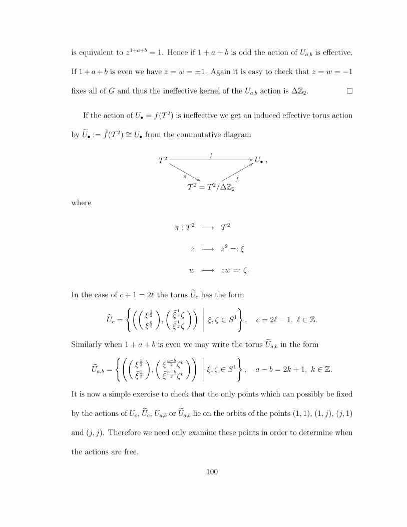
is equivalent to z1+a+b = 1. Hence if 1 + a + b is odd the action of Ua,b is effective.

If 1 + a + b is even we have z = w = ±1. Again it is easy to check that z = w = −1

fixes all of G and thus the ineffective kernel of the Ua,b action is ∆Z2.

If the action of U• = f(T 2) is ineffective we get an induced effective torus action

by U• := f(T 2) ∼= U• from the commutative diagram

T 2f //

π &&MMMMMMMMMMM U•

T 2 = T 2/∆Z2

f

88qqqqqqqqqqq

,

where

π : T 2 −→ T 2

z 7−→ z2 =: ξ

w 7−→ zw =: ζ.

In the case of c + 1 = 2` the torus Uc has the form

Uc =

((ξ

12

ξc2

),

(ξ

12 ζ

ξ12 ζ

)) ∣∣∣∣∣ ξ, ζ ∈ S1

, c = 2`− 1, ` ∈ Z.

Similarly when 1 + a + b is even we may write the torus Ua,b in the form

Ua,b =

((ξ

12

ξ12

),

(ξ

a−b2 ζb

ξa−b2 ζb

)) ∣∣∣∣∣ ξ, ζ ∈ S1

, a− b = 2k + 1, k ∈ Z.

It is now a simple exercise to check that the only points which can possibly be fixed

by the actions of Uc, Uc, Ua,b or Ua,b lie on the orbits of the points (1, 1), (1, j), (j, 1)

and (j, j). Therefore we need only examine these points in order to determine when

the actions are free.

100

Lemma 6.1.2. The action of Uc, c even, is free if and only if c = 0. The action of

Uc, c odd, is never free.

Proof. Consider first the action of Uc for c even. By the discussion above and from

equation (6.1.4) we find that

(1, 1) fixed ⇐⇒ zw = 1 & zcw = 1 ⇐⇒ z = w & zc−1 = 1;

(1, j) fixed ⇐⇒ zw = 1 & zcw = 1 ⇐⇒ z = w & zc+1 = 1;

(j, 1) fixed ⇐⇒ zw = 1 & zcw = 1 ⇐⇒ z = w & zc+1 = 1;

(j, j) fixed ⇐⇒ zw = 1 & zcw = 1 ⇐⇒ z = w & zc−1 = 1.

Thus we see that the action is free if and only if c ± 1 = ±1. But c is even and

hence c = 0 is the only value for which we obtain a free action.

Consider now Uc for c odd. We again apply equation (6.1.4) and find

(1, 1) fixed ⇐⇒ ξζ = 1 & ξc+12 ζ = 1 ⇐⇒ ξ = ζ & ξ

c−12 = 1;

(1, j) fixed ⇐⇒ ξζ = 1 & ξc−12 ζ = 1 ⇐⇒ ξ = ζ & ξ

c+12 = 1;

(j, 1) fixed ⇐⇒ ζ = 1 & ξc+12 ζ = 1 ⇐⇒ ζ = 1 & ξ

c+12 = 1;

(j, j) fixed ⇐⇒ ξζ = 1 & ξc−12 ζ = 1 ⇐⇒ ζ = 1 & ξ

c−12 = 1.

Therefore the action is free (namely ξ = ζ = 1 in each case) if and only if c±12

= ±1,

i.e. if and only if c±1 = ±2. But c is odd and there is no value for which we obtain

both c + 1 = ±2 and c − 1 = ±2. Hence we will always have a fixed point and so

the action of Uc, c odd, is never free.

101

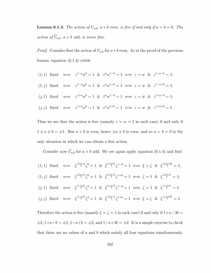
Lemma 6.1.3. The action of Ua,b, a + b even, is free if and only if a = b = 0. The

action of Ua,b, a + b odd, is never free.

Proof. Consider first the action of Ua,b for a+b even. As in the proof of the previous

lemma, equation (6.1.4) yields

(1, 1) fixed ⇐⇒ z1−awb = 1 & zaw1−b = 1 ⇐⇒ z = w & z1−a−b = 1;

(1, j) fixed ⇐⇒ z1−awb = 1 & zaw1+b = 1 ⇐⇒ z = w & z1−a+b = 1;

(j, 1) fixed ⇐⇒ z1+awb = 1 & zaw1−b = 1 ⇐⇒ z = w & z1+a−b = 1;

(j, j) fixed ⇐⇒ z1+awb = 1 & zaw1+b = 1 ⇐⇒ z = w & z1+a+b = 1.

Thus we see that the action is free (namely z = w = 1 in each case) if and only if

1 ± a ± b = ±1. But a + b is even, hence ±a ± b is even, and so a = b = 0 is the

only situation in which we can obtain a free action.

Consider now Ua,b for a + b odd. We yet again apply equation (6.1.4) and find

(1, 1) fixed ⇐⇒ ξ1+a−b

2 ζb = 1 & ξ1−a+b

2 ζ1−b = 1 ⇐⇒ ξ = ζ & ξ1+a−3b

2 = 1;

(1, j) fixed ⇐⇒ ξ1+a−b

2 ζb = 1 & ξ1+a−b

2 ζ1+b = 1 ⇐⇒ ζ = 1 & ξ1+a−b

2 = 1;

(j, 1) fixed ⇐⇒ ξ1−a+b

2 ζb = 1 & ξ1−a+b

2 ζ1−b = 1 ⇐⇒ ζ = 1 & ξ1−a+b

2 = 1;

(j, j) fixed ⇐⇒ ξ1−a+b

2 ζb = 1 & ξ1+a−b

2 ζ1+b = 1 ⇐⇒ ξ = ζ & ξ1−a+3b

2 = 1.

Therefore the action is free (namely ξ = ζ = 1 in each case) if and only if 1+a−3b =

±2, 1+a−b = ±2, 1−a+b = ±2, and 1−a+3b = ±2. It is a simple exercise to check

that there are no values of a and b which satisfy all four equations simultaneously.

102

Hence we will always have a fixed point and so the action of Ua,b, a+ b odd, is never

free.

If we combine the last two lemmas we notice that we have in fact proved:

Proposition 6.1.4. Up to a change of coordinates or reordering of factors, the only

free T 2 actions on S3 × S3 which are diagonal on the right are given by UL = Ua,b,

a = b = 0, and Uc, c = 0. The actions are, respectively,

(z, w) ?

(q1

q2

)=

(zq1

wq2

), z, w ∈ S1, q1, q2 ∈ S3; and (6.1.5)

(z, w) ?

(q1

q2

)=

(zq1w

q2w

), z, w ∈ S1, q1, q2 ∈ S3. (6.1.6)

The resulting manifolds are S2 × S2, CP 2#− CP 2 respectively.

For those actions which are not free we may consider the equations obtained in

the proofs of Lemmas 6.1.2 and 6.1.3 in order to write down explicitly the isotropy

groups Γ(q1,q2) of singular points, which we recall can only be the T 2-orbits of the

points (q1, q2) = (1, 1), (1, j), (j, 1), (j, j) ∈ S3 × S3. The isotropy groups for each

action are collected in Table 6.1. By considering the groups in this table we can

easily find examples which have only one or two singular points and small isotropy

groups at these points. In the event that they arise, Z0 and Z1 denote S1 and 1

respectively. We include some examples in Tables 6.2, 6.3, 6.4 and 6.5.

103

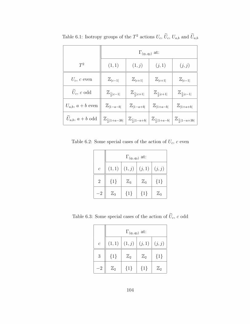
Table 6.1: Isotropy groups of the T 2 actions Uc, Uc, Ua,b and Ua,b

Γ(q1,q2) at:

T 2 (1, 1) (1, j) (j, 1) (j, j)

Uc, c even Z|c−1| Z|c+1| Z|c+1| Z|c−1|

Uc, c odd Z 12|c−1| Z 1

2|c+1| Z 1

2|c+1| Z 1

2|c−1|

Ua,b, a + b even Z|1−a−b| Z|1−a+b| Z|1+a−b| Z|1+a+b|

Ua,b, a + b odd Z 12|1+a−3b| Z 1

2|1−a+b| Z 1

2|1+a−b| Z 1

2|1−a+3b|

Table 6.2: Some special cases of the action of Uc, c even

Γ(q1,q2) at:

c (1, 1) (1, j) (j, 1) (j, j)

2 1 Z3 Z3 1

−2 Z3 1 1 Z3

Table 6.3: Some special cases of the action of Uc, c odd

Γ(q1,q2) at:

c (1, 1) (1, j) (j, 1) (j, j)

3 1 Z2 Z2 1

−2 Z2 1 1 Z2

104

Table 6.4: Some special cases of the action of Ua,b, a + b even

Γ(q1,q2) at:

(a, b) (1, 1) (1, j) (j, 1) (j, j)

(1, 1) 1 1 1 Z3

(1,−1) 1 1 Z3 1

(−1, 1) 1 Z3 1 1

(−1,−1) Z3 1 1 1

Table 6.5: Some special cases of the action of Ua,b, a + b odd

Γ(q1,q2) at:

(a, b) (1, 1) (1, j) (j, 1) (j, j)

(−6,−3) Z2 Z2 1 1

(3, 0) Z2 1 Z2 1

(−3, 0) 1 Z2 1 Z2

(6, 3) 1 1 Z2 Z2

105

6.2 Curvature on (S3 × S3)//T 2

Let K = ∆S3 ⊂ G = S3 × S3, and let 〈 , 〉0 be the bi-invariant product metric on

G. The Lie algebras of G and K are denoted g and k respectively. Then g = k⊕ p,

where p is the orthogonal complement to k with respect to 〈 , 〉0. Notice that (g, k)

is a rank one symmetric pair. Define a new left-invariant, right K-invariant metric

on G via:

〈X, Y 〉1 = 〈X, Φ(Y )〉0,

where Φ(Y ) = Yp + λYk, λ ∈ (0, 1). By Lemma 2.2.2 we know that a plane σ =

Span Φ−1(X), Φ−1(Y ) ⊂ g has zero-curvature with respect to 〈 , 〉1 if and only if

0 = [X,Y ] = [Xp, Yp] = [Xk, Yk].

Hence, for G and K as above, a zero-curvature plane must be of the form

σ = Span Φ−1(v, 0), Φ−1(0, v) | v ∈ Im H. (6.2.1)

Since we are considering T 2 actions which are diagonal on the right of G, it is clear

that the actions are by isometries and hence induce a metric on G//T 2.

Theorem 6.2.1. (G, 〈 , 〉1)//T 2 has almost positive curvature if and only if the

action is not free.

Proof. By O’Neill’s formula it is sufficient to show that points in G with horizontal

zero-curvature planes lie on a hypersurface. Recall that the existence of an ineffec-

tive kernel will have no impact on our curvature computations. We therefore need

106

only consider torus actions of the form

Ua,b =

((z

w

),

(zawb

zawb

)) ∣∣∣ z, w ∈ S1

, a, b ∈ Z;

Uc =

((z

zc

),

(w

w

)) ∣∣∣ z, w ∈ S1

, c ∈ Z,

and notice that the UL action of (6.1.1) is the special case (a, b) = (0, 0) of Ua,b.

Consider first the action by Ua,b. The vertical subspace at (q1, q2), left translated

to (1, 1), is given by

V(q1,q2) =

1

2

(θ Adq1 i− (aθ + bϕ)i

ϕ Adq2 i− (aθ + bϕ)i

) ∣∣∣∣∣ θ, ϕ ∈ R

.

Thus the horizontal subspace with respect to 〈 , 〉1 is

H(q1,q2) =

Φ−1(v, w)

∣∣∣∣∣Adq1 v − a(v + w) ⊥ i

Adq2 w − b(v + w) ⊥ i

.

Hence, by equation (6.2.1), a zero-curvature plane σ = Span Φ−1(v, 0), Φ−1(0, v)

is horizontal if and only if

Adq1 v − av ⊥ i, (6.2.2)

av ⊥ i, (6.2.3)

Adq2 v − bv ⊥ i, and (6.2.4)

bv ⊥ i. (6.2.5)

We want to show that v, Adq1 v, Adq2 v ⊥ i since this is equivalent to v ⊥ i, Adq1 i,

Adq2 i. This will imply that v = 0 unless i, Adq1 i, and Adq2 i are linearly dependent,

which in turn would imply positive curvature at the point [(q1, q2)] ∈ G//Ua,b. It is

107

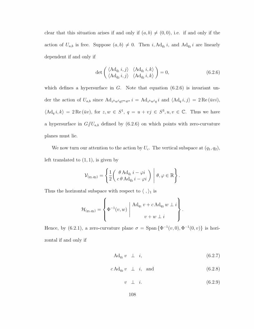
clear that this situation arises if and only if (a, b) 6= (0, 0), i.e. if and only if the

action of Ua,b is free. Suppose (a, b) 6= 0. Then i, Adq1 i, and Adq2 i are linearly

dependent if and only if

det

( 〈Adq1 i, j〉 〈Adq1 i, k〉〈Adq2 i, j〉 〈Adq2 i, k〉

)= 0, (6.2.6)

which defines a hypersurface in G. Note that equation (6.2.6) is invariant un-

der the action of Ua,b since Adzkw`qzmwn i = Adzkw`q i and 〈Adq i, j〉 = 2 Re (uvi),

〈Adq i, k〉 = 2 Re (uv), for z, w ∈ S1, q = u + vj ∈ S3, u, v ∈ C. Thus we have

a hypersurface in G//Ua,b defined by (6.2.6) on which points with zero-curvature

planes must lie.

We now turn our attention to the action by Uc. The vertical subspace at (q1, q2),

left translated to (1, 1), is given by

V(q1,q2) =

1

2

(θ Adq1 i− ϕi

c θ Adq2 i− ϕi

) ∣∣∣∣∣ θ, ϕ ∈ R

.

Thus the horizontal subspace with respect to 〈 , 〉1 is

H(q1,q2) =

Φ−1(v, w)

∣∣∣∣∣Adq1 v + c Adq2 w ⊥ i

v + w ⊥ i

.

Hence, by (6.2.1), a zero-curvature plane σ = Span Φ−1(v, 0), Φ−1(0, v) is hori-

zontal if and only if

Adq1 v ⊥ i, (6.2.7)

c Adq2 v ⊥ i, and (6.2.8)

v ⊥ i. (6.2.9)

108

It is clear that the only situation in which we do not get v, Adq1 v, Adq2 v ⊥ i is

when c = 0, i.e. when the action is free. In all other situations we have almost

positive curvature by the same argument as for Ua,b.

Remark 6.2.2. In all cases we get a horizontal zero-curvature plane at (q1, q2) if

either

• Adq1 i = ±i ⇐⇒ q1 ∈ C or Cj,

• Adq2 i = ±i ⇐⇒ q2 ∈ C or Cj, or

• Adq1 i = ±Adq2 i ⇐⇒ q1 ⊥ q2, iq2 or q1 ⊥ jq2, kq2.

Thus we will always have a zero-curvature plane at the singular points when the

action is not free. Moreover, in the free cases we have a zero-curvature plane at

every point. More precisely:

• The action Ua,b with a = b = 0 yields Adq1 i, Adq2 i ⊥ v, which implies that

there is a unique horizontal zero-curvature plane when Adq1 i and Adq2 i are

linearly independent, and there is an S1 worth of zero-curvature planes when

Adq1 i = ±Adq2 i, i.e. when q1 ⊥ q2, iq2 or q1 ⊥ jq2, kq2;

• The action Uc with c = 0 yields i, Adq1 i ⊥ v, which implies that there is a

unique horizontal zero-curvature plane when q1 6∈ C or Cj, and there is an S1

worth of zero-curvature planes when q1 ∈ C or Cj.

109

Bibliography

[AW] S. Aloff, N. Wallach, An infinite family of 7-manifolds admitting positively

curved Riemannian structures, Bull. Amer. Math. Soc. 81 (1975), 93-97

[AMP1] L. Astey, E. Micha and G. Pastor, Homeomorphism and diffeomorphism

types of Eschenburg spaces, Differential Geom. Appl. 7 (1997), 41-50

[AMP2] L. Astey, E. Micha and G. Pastor, On the homotopy type of Eschenburg

spaces with positive sectional curvature, Proc. Amer. Math. Soc. 132 (2004),

No. 12, 3725-3729

[Au] T. Aubin, Metriques riemanniennes et courbure, J. Diff. Geom. 4 (1970),

383-424

[Ba1] Y. Bazaikin, On a certain family of closed 13-dimensional Riemannian man-

ifolds of positive curvature, Sib. Math. J. 37 No. 6 (1996), 1219-1237

[BB] L. Berard-Bergery, Les varietes riemanniennes homogenes simplement con-

nexes de dimension impaire a courbure strictement positive, J. Math. pure et

appl. 55 (1976), 47-68

110

[Ber1] M. Berger, Les varietes riemanniennes 1/4-pincees, Ann. Scuola Norm. Sup.

Pisa 14 (1960), 161-170

[Ber2] M. Berger, Les varietes riemanniennes homogenes normales simplement con-

nexes a courbure strictement positive, Ann. Scuola Norm. Sup. Pisa 15 (1961),

179-246

[Bo] R. Bock, Doppelquotienten ungerader dimension und positive Schnit-

tkrummung, Dissertation, University of Augsburg, 1998

[BH] A. Borel and F. Hirzebruch, Characteristic classes and homogeneous spaces,

I, Amer. J. Math. 80 (1958), 458-538

[BS1] S. Brendle and R. Schoen, Manifolds with 1/4-pinched Curvature are Space

Forms, preprint 2007

[BS2] S. Brendle and R. Schoen, Classification of manifolds with weakly 1/4-pinched

curvatures, preprint 2007

[Br] E. H. Brown, Jr., The cohomology of BSO(n) and BO(n) with integer coeffi-

cients, Proc. Amer. Math. Soc. 83 (1982), No. 2, 283-288

[CMV] M. Cadek, M. Mimura and J. Vanzura, The cohomology rings of real Stiefel

manifolds with integer coefficients, J. Math. Kyoto Univ. 43 (2003), No. 2,

425-442

111

[Ch] J. Cheeger, Some examples of manifolds of nonnegative curvature, J. Diff.

Geom. 8 (1973), 623 - 628

[CEZ] T. Chinberg, C. Escher and W. Ziller, Topological properties of Eschenburg

spaces and 3-Sasakian manifolds, Math. Ann. 339(1) (2007), 3 - 20

[Eh] P. Ehrlich, Metric deformations of curvature I, Geom. Dedicata 5 (1976),

1-23

[E1] J.-H. Eschenburg, Freie isometrische Aktionen auf kompakten Liegruppen mit

positiv gekrummten Orbitraumen, Schriftenreihe Math. Inst. Univ. Munster

(2) 32 (1984)

[E2] J.-H. Eschenburg, Cohomology of biquotients, Manuscripta Math. 75 (1992),

151-166

[E3] J.-H. Eschenburg, Almost positive curvature on the Gromoll-Meyer 7-sphere,

Proc. Amer. Math. Soc. 130 (2002), No. 4, 1165 - 1167

[EK] J.-H. Eschenburg and M. Kerin, Almost positive curvature on the Gromoll-

Meyer 7-sphere, Proc. Amer. Math. Soc., to appear

[EKS] J.-H. Eschenburg, A. Kollross and K. Shankar, Free, isometric circle actions

on compact symmetric spaces, Geom. Dedicata 102 (2003), 35-44

[F] M. Feshbach, The integral cohomology rings of the classifying spaces of O(n)

and SO(n), Indiana Univ. Math. J. 32 (1983), 511-516

112

[FZ1] L. Florit and W. Ziller, On the topology of positively curved Bazaikin spaces,

J. Europ. Math. Soc., to appear

[FZ2] L. Florit and W. Ziller, Orbifold fibrations of Eschenburg spaces, Geom. Ded-

icata 127 (2007), 159 - 175

[GWZ] H. Gluck, F. Warner and W. Ziller, The geometry of the Hopf fibrations,

Enseign. Math. 32 (1986), 173 - 198

[GM] D. Gromoll and W.T. Meyer, An exotic sphere with nonnegative sectional

curvature, Ann. of Math. 100 (1974), 401 - 406

[GSZ] K. Grove, K. Shankar and W. Ziller, Symmetries of Eschenburg spaces and

the Chern problem, Asian J. Math. 10 (2006) No. 3, 647-662

[GZ1] K. Grove and W. Ziller: Curvature and symmetry of Milnor spheres, Ann.

of Math. 152 (2000), 331-367

[GZ2] K. Grove and W. Ziller: Lifting group actions and non-negative curvature,

preprint 2008

[Ha] R. Hamilton, Three manifolds with positive Ricci curvature, J. Diff. Geom. 17

(1982), 255-306

[J] N. Jacobson, Some groups of transformations defined by Jordan algebras, I,

J. Reine Angew. Math. 204 (1960), 74-98

113

[KZ] V. Kapovitch and W. Ziller, Biquotients with singly generated rational coho-

mology, Geom. Dedicata 104 (2004), 149-160

[K] W. Klingenberg, Uber Riemannsche mannigfaltigkeiten mit positiver

krummung, Comment. Math. Helv. 35 (1961), 47-54

[KS1] M. Kreck and S. Stolz, Some non-diffeomorphic homeomorphic 7-manifolds

with positive sectional curvature, J. Diff. Geom. 33 (1991) 465-486

[KS2] M. Kreck and S. Stolz, A correction on: “Some non-diffeomorphic home-

omorphic 7-manifolds with positive sectional curvature”, J. Diff. Geom. 49

(1998) 203-204

[K1] B. Kruggel, A homotopy classification of certain 7-manifolds, Trans. Amer.

Math. Soc. 349(7) (1997), 2827-2843

[K2] B. Kruggel, Homeomorphism and diffeomorphism classification of Eschenburg

spaces, Quart. J. Math. 56 (2005), 553-577

[MT] M. Mimura and H. Toda, Topology of Lie groups I, II, Translations of Math-

ematical Monographs 91, Amer. Math. Soc., Providence, RI, 1991

[Mo] L. J. Mordell, Diophantine Equations, Academic Press, London and New York

(1969)

114

[M] S. Murakami, Exceptional simple Lie groups and related topics in recent differ-

ential geometry, Differential geometry and topology (Tianjin, 1986-87), 183-

221, Lecture Notes in Math., 1369, Springer, Berlin, 1989

[Mu] P. Muter, Krummungserhohende Deformationen mittels Gruppenaktionen,

Ph.D. thesis, University of Munster, 1987

[NW] L. Ni and J. Wolfson, Positive complex sectional curvature, Ricci flow and

the differential sphere theorem, preprint 2007

[Pe] G. Perelman, Proof of the soul conjecture of Cheeger and Gromoll, J. Diff.

Geom. 40 (1994) 209-212

[PW] P. Petersen and F. Wilhelm, Examples of Riemannian manifolds with positive

curvature almost everywhere, Geom. and Top. 3 (1999), 331-367

[Sh2] K. Shankar, Strong inhomogeneity of Eschenburg spaces (with an appendix by

M. Dickinson and K. Shankar, Mich. Math. J. 50 (2002), 125-142

[Si] W. Singhof, On the topology of double coset manifolds, Math. Ann. 297(1)

(1993), 133-146

[Sp] E. H. Spanier, Algebraic topology, Springer 1981

[T] I. A. Taimanov, On totally geodesic embeddings of 7-dimensional manifolds

in 13-dimensional manifolds of positive sectional curvature, Sib. Math. 187

(1996), 1853-1867

115

[Ta1] K. Tapp, Quasi-positive curvature on homogeneous bundles, J. Diff. Geom.

65 (2003), 273-287

[Ta2] K. Tapp, Flats in Riemannian submersions from Lie groups, Preprint 2007,

DG0703389

[To] B. Totaro, Cheeger Manifolds and the Classification of Biquotients, J. Diff.

Geom. 61 (2002), 397-451

[Wa] N. Wallach, Compact homogeneous Riemannian manifolds with strictly posi-

tive curvature, Ann. of Math. 96 (1972), 277-295

[Wh] G. W. Whitehead, Elements of homotopy theory, Springer 1978

[W] F. Wilhelm, An exotic sphere with positive curvature almost everywhere, J.

Geom. Anal. 11 (2001), 519 - 560

[Wi] B. Wilking, Manifolds with positive sectional curvature almost everywhere,

Invent. Math. 148 (2002), 117-141

[Zi1] W. Ziller, Homogeneous spaces, biquotients, and manifolds with positive cur-

vature, Lecture Notes 1998, unpublished

[Zi2] W. Ziller, On Eschenburg’s Habilitation on biquotients, Lecture Notes 2007,

unpublished

116