birational classiï¬cation of varieties
TRANSCRIPT

Birational classification of varietiesJames McKernan
UCSB
Birational classification of varieties – p.1

A little category theory
The most important part of any category C are themorphisms not the objects.
It is the aim of higher dimensional geometry toclassify algebraic varieties up to birationalequivalence.
Thus the objects are algebraic varieties, but what arethe morphisms?
Birational classification of varieties – p.2

Contraction mappings
Well, given any morphism f : X −→ Y of normalalgebraic varieties, we can always factor f asg : X −→ W and h : W −→ Y , where h is finiteand g has connected fibres.
Mori theory does not say much about finite maps.
It does have a lot to say about morphisms withconnected fibres.
In fact any morphism f : X −→ Y such thatf∗OX = OY will be called a contraction morphism.If X and Y are normal, this is the same as requiringthe fibres of f to be connected.
Birational classification of varieties – p.3

Curves versus divisors
So we are interested in the category of algebraicvarieties (primarily normal and projective), andcontraction morphisms, and we want to classify allcontraction morphisms.
Traditionally the approved way to study a projectivevariety is to embed it in projective space, andconsider the family of hyperplane sections.
In Mori theory, we focus on curves, not divisors.
In fact a contraction morphism f : X −→ Y isdetermined by the curves which it contracts. IndeedY is clearly determined topologically, and thecondition OY = f∗OX determines the algebraicstructure.
Birational classification of varieties – p.4

The closed cone of curves
NE(X) denotes the cone of effective curves of X ,the closure of the image of the effective curves inH2(X, R), considered as a cone inside the span.
By Kleiman’s criteria, any divisor H is ample iff itdefines a positive linear functional on
NE(X) − {0} by
[C] −→ H · C.
Given f , set D = f ∗H , where H is an ample divisoron Y . Then D is nef, that is D · C ≥ 0, for everycurve C.
Birational classification of varieties – p.5
Semiample divisors
Then a curve C is contracted by f iff D · C = 0.Moreover the set of such curves is a face of NE(X).
Thus there is partial correspondence between the
• faces F of NE(X) and the
• contraction morphisms f .
So, which faces F correspond to contractions f?Similarly which divisors are the pullback of ampledivisors?
We say that a divisor D is semiample if D = f ∗H ,for some contraction morphism f and ample divisorH .
Note that if D is semiample, it is certainly nef.
Birational classification of varieties – p.6

Semiample divisors
Then a curve C is contracted by f iff D · C = 0.Moreover the set of such curves is a face of NE(X).
Thus there is partial correspondence between the
• faces F of NE(X) and the
• contraction morphisms f .
So, which faces F correspond to contractions f?Similarly which divisors are the pullback of ampledivisors?
We say that a divisor D is semiample if D = f ∗H ,for some contraction morphism f and ample divisorH .
Note that if D is semiample, it is certainly nef.Birational classification of varieties – p.6

An easy example
Suppose that X = P1 × P1.
NE(X) sits inside a two dimensional vector space.The cone is spanned by f1 = [P1 × {pt}] andf2 = [{pt} × P1].
This cone has four faces. The whole cone, the zerocone and the two cones spanned by f1 and f2.
The corresponding morphisms are the identity, theconstant map to a point, and the two projections.
In this example, the correspondence between facesand contractions is complete and in fact every nefdivisor is semiample.
Birational classification of varieties – p.7

A harder example
Suppose that X = E × E, where E is a generalelliptic curve.
NE(X) sits inside a three dimensional vector space.The class δ of the diagonal is independent from theclasses f1 and f2 of the two fibres.
Aut(X) is large; it contains SL(2, Z).
There are many contractions. Start with either of thetwo projections and act by Aut(X).
Birational classification of varieties – p.8

NE(E × E)
On a surface, if D2 > 0, and D · H > 0 for someample divisor, then D is effective by Riemann-Roch.
As the action of Aut(X) is transitive, there are nocurves of negative self-intersection. Thus NE(X) isgiven by D2 ≥ 0, D · H ≥ 0.
NE(X) is one half of the classic circular conex2 + y2 = z2 ⊂ R3. Thus many faces don’tcorrespond to contractions.
Many nef divisors are not semiample. Indeed, evenon an elliptic curve there are numerically trivialdivisors which are not torsion.
Birational classification of varieties – p.9

A much harder example
Suppose that X = C2, C × C, modulo the obviousinvolution, where C is a general curve, g ≥ 2.
C2 corresponds to divisors p + q of degree 2.
NE(X) sits inside a two dimensional vector space,spanned by the image δ of the class of the diagonaland the image f of the class of a fibre. In particularthe cone is spanned by two rays.
One contraction is given by the Abel-Jacobi map,and there is a similar map which contracts δ.
But what happens when g and d are both large?
Birational classification of varieties – p.10

More Pathologies
If S −→ C is the projectivisation of a stable ranktwo vector bundle over a curve of genus g ≥ 2, thenNE(S) sits inside a two dimensional vector space.
One edge is spanned by the class f of a fibre. Theother edge is corresponds to a class α ofself-intersection zero.
However there is no curve Σ such that the class of Cis equal to α.
Indeed the existence of such a curve would implythat the pullback of S along Σ −→ C splits, whichcontradicts stability.
We really need to take the closure, to define NE(S).
Birational classification of varieties – p.11

More Pathologies
If S −→ C is the projectivisation of a stable ranktwo vector bundle over a curve of genus g ≥ 2, thenNE(S) sits inside a two dimensional vector space.
One edge is spanned by the class f of a fibre. Theother edge is corresponds to a class α ofself-intersection zero.
However there is no curve Σ such that the class of Cis equal to α.
Indeed the existence of such a curve would implythat the pullback of S along Σ −→ C splits, whichcontradicts stability.
We really need to take the closure, to define NE(S).Birational classification of varieties – p.11

Even more Pathologies
Let S −→ P2 be the blow up of P2 at 9 generalpoints.
We can perturb one point, so that the nine points arethe intersection of two smooth cubics.
In this case S −→ P1, with elliptic fibres.
The nine exceptional divisors are sections. Thedifference of any two is not torsion in the genericfibre. Translating by the difference generatesinfinitely many exceptional divisors.
Perturbing, we lose the fibration, but keep the−1-curves.
What went wrong?
Birational classification of varieties – p.12
Even more Pathologies
Let S −→ P2 be the blow up of P2 at 9 generalpoints.
We can perturb one point, so that the nine points arethe intersection of two smooth cubics.
In this case S −→ P1, with elliptic fibres.
The nine exceptional divisors are sections. Thedifference of any two is not torsion in the genericfibre. Translating by the difference generatesinfinitely many exceptional divisors.
Perturbing, we lose the fibration, but keep the−1-curves.
What went wrong?Birational classification of varieties – p.12
The canonical divisor
The answer in all cases is to consider the behaviourof the canonical divisor KX .
Recall that the canonical divisor is defined bypicking a meromorphic section of ∧nT ∗
X, and
looking at is zeroes minus poles.
The basic moral is that the cone of curves is nice onthe negative side, and that if we contract thesecurves, we get a reasonable model.
Consider the case of curves.
Birational classification of varieties – p.13

Smooth projective curves
Curves C come in three types:
• C ' P1. KC is negative.
• C is elliptic, a plane cubic. KC is zero.
• C has genus at least two. KC is positive.
We hope (wishfully?) that the same pattern remainsin higher dimensions.
So let us now consider surfaces.
Birational classification of varieties – p.14

Smooth projective curves
Curves C come in three types:
• C ' P1.
KC is negative.
• C is elliptic, a plane cubic. KC is zero.
• C has genus at least two. KC is positive.
We hope (wishfully?) that the same pattern remainsin higher dimensions.
So let us now consider surfaces.
Birational classification of varieties – p.14

Smooth projective curves
Curves C come in three types:
• C ' P1. KC is negative.
• C is elliptic, a plane cubic. KC is zero.
• C has genus at least two. KC is positive.
We hope (wishfully?) that the same pattern remainsin higher dimensions.
So let us now consider surfaces.
Birational classification of varieties – p.14

Smooth projective curves
Curves C come in three types:
• C ' P1. KC is negative.
• C is elliptic, a plane cubic.
KC is zero.
• C has genus at least two. KC is positive.
We hope (wishfully?) that the same pattern remainsin higher dimensions.
So let us now consider surfaces.
Birational classification of varieties – p.14

Smooth projective curves
Curves C come in three types:
• C ' P1. KC is negative.
• C is elliptic, a plane cubic. KC is zero.
• C has genus at least two. KC is positive.
We hope (wishfully?) that the same pattern remainsin higher dimensions.
So let us now consider surfaces.
Birational classification of varieties – p.14

Smooth projective curves
Curves C come in three types:
• C ' P1. KC is negative.
• C is elliptic, a plane cubic. KC is zero.
• C has genus at least two.
KC is positive.
We hope (wishfully?) that the same pattern remainsin higher dimensions.
So let us now consider surfaces.
Birational classification of varieties – p.14

Smooth projective curves
Curves C come in three types:
• C ' P1. KC is negative.
• C is elliptic, a plane cubic. KC is zero.
• C has genus at least two. KC is positive.
We hope (wishfully?) that the same pattern remainsin higher dimensions.
So let us now consider surfaces.
Birational classification of varieties – p.14

Smooth projective curves
Curves C come in three types:
• C ' P1. KC is negative.
• C is elliptic, a plane cubic. KC is zero.
• C has genus at least two. KC is positive.
We hope (wishfully?) that the same pattern remainsin higher dimensions.
So let us now consider surfaces.
Birational classification of varieties – p.14

Smooth projective surfaces
Any smooth surface S is birational to:
• P2. −KS is ample, a Fano variety.
• S −→ C, g(C) ≥ 1, where the fibres are isomorphicto P1. −KS is relatively ample, a Fano fibration.
• S −→ C, where KS is zero on the fibres. If C is acurve, the fibres are elliptic curves.
• KS is ample. S is of general type. Note that S isforced to be singular in general.
The problem, as we have already seen, is that we candestroy this picture, simply by blowing up. It is theaim of the MMP to reverse the process of blowingup.
Birational classification of varieties – p.15

Smooth projective surfaces
Any smooth surface S is birational to:
• P2.
−KS is ample, a Fano variety.
• S −→ C, g(C) ≥ 1, where the fibres are isomorphicto P1. −KS is relatively ample, a Fano fibration.
• S −→ C, where KS is zero on the fibres. If C is acurve, the fibres are elliptic curves.
• KS is ample. S is of general type. Note that S isforced to be singular in general.
The problem, as we have already seen, is that we candestroy this picture, simply by blowing up. It is theaim of the MMP to reverse the process of blowingup.
Birational classification of varieties – p.15

Smooth projective surfaces
Any smooth surface S is birational to:
• P2. −KS is ample, a Fano variety.
• S −→ C, g(C) ≥ 1, where the fibres are isomorphicto P1. −KS is relatively ample, a Fano fibration.
• S −→ C, where KS is zero on the fibres. If C is acurve, the fibres are elliptic curves.
• KS is ample. S is of general type. Note that S isforced to be singular in general.
The problem, as we have already seen, is that we candestroy this picture, simply by blowing up. It is theaim of the MMP to reverse the process of blowingup.
Birational classification of varieties – p.15
Smooth projective surfaces
Any smooth surface S is birational to:
• P2. −KS is ample, a Fano variety.
• S −→ C, g(C) ≥ 1, where the fibres are isomorphicto P1.
−KS is relatively ample, a Fano fibration.
• S −→ C, where KS is zero on the fibres. If C is acurve, the fibres are elliptic curves.
• KS is ample. S is of general type. Note that S isforced to be singular in general.
The problem, as we have already seen, is that we candestroy this picture, simply by blowing up. It is theaim of the MMP to reverse the process of blowingup.
Birational classification of varieties – p.15

Smooth projective surfaces
Any smooth surface S is birational to:
• P2. −KS is ample, a Fano variety.
• S −→ C, g(C) ≥ 1, where the fibres are isomorphicto P1. −KS is relatively ample, a Fano fibration.
• S −→ C, where KS is zero on the fibres. If C is acurve, the fibres are elliptic curves.
• KS is ample. S is of general type. Note that S isforced to be singular in general.
The problem, as we have already seen, is that we candestroy this picture, simply by blowing up. It is theaim of the MMP to reverse the process of blowingup.
Birational classification of varieties – p.15

Smooth projective surfaces
Any smooth surface S is birational to:
• P2. −KS is ample, a Fano variety.
• S −→ C, g(C) ≥ 1, where the fibres are isomorphicto P1. −KS is relatively ample, a Fano fibration.
• S −→ C, where KS is zero on the fibres.
If C is acurve, the fibres are elliptic curves.
• KS is ample. S is of general type. Note that S isforced to be singular in general.
The problem, as we have already seen, is that we candestroy this picture, simply by blowing up. It is theaim of the MMP to reverse the process of blowingup.
Birational classification of varieties – p.15

Smooth projective surfaces
Any smooth surface S is birational to:
• P2. −KS is ample, a Fano variety.
• S −→ C, g(C) ≥ 1, where the fibres are isomorphicto P1. −KS is relatively ample, a Fano fibration.
• S −→ C, where KS is zero on the fibres. If C is acurve, the fibres are elliptic curves.
• KS is ample. S is of general type. Note that S isforced to be singular in general.
The problem, as we have already seen, is that we candestroy this picture, simply by blowing up. It is theaim of the MMP to reverse the process of blowingup.
Birational classification of varieties – p.15

Smooth projective surfaces
Any smooth surface S is birational to:
• P2. −KS is ample, a Fano variety.
• S −→ C, g(C) ≥ 1, where the fibres are isomorphicto P1. −KS is relatively ample, a Fano fibration.
• S −→ C, where KS is zero on the fibres. If C is acurve, the fibres are elliptic curves.
• KS is ample.
S is of general type. Note that S isforced to be singular in general.
The problem, as we have already seen, is that we candestroy this picture, simply by blowing up. It is theaim of the MMP to reverse the process of blowingup.
Birational classification of varieties – p.15

Smooth projective surfaces
Any smooth surface S is birational to:
• P2. −KS is ample, a Fano variety.
• S −→ C, g(C) ≥ 1, where the fibres are isomorphicto P1. −KS is relatively ample, a Fano fibration.
• S −→ C, where KS is zero on the fibres. If C is acurve, the fibres are elliptic curves.
• KS is ample. S is of general type. Note that S isforced to be singular in general.
The problem, as we have already seen, is that we candestroy this picture, simply by blowing up. It is theaim of the MMP to reverse the process of blowingup.
Birational classification of varieties – p.15

Smooth projective surfaces
Any smooth surface S is birational to:
• P2. −KS is ample, a Fano variety.
• S −→ C, g(C) ≥ 1, where the fibres are isomorphicto P1. −KS is relatively ample, a Fano fibration.
• S −→ C, where KS is zero on the fibres. If C is acurve, the fibres are elliptic curves.
• KS is ample. S is of general type. Note that S isforced to be singular in general.
The problem, as we have already seen, is that we candestroy this picture, simply by blowing up. It is theaim of the MMP to reverse the process of blowingup.
Birational classification of varieties – p.15

The cone theorem
Let X be a smooth variety, or in general mildlysingular. There are two cases:
• KX is nef.
• There is a curve C such that KX · C < 0.
In the second case there is a KX-extremal ray R.That is to say R is extremal in the sense of convexgeometry, and KX · R < 0.
Moreover, we can contract R, φR : X −→ Y .
φR is a contraction morphism, −KX is relativelyample, and the relative Picard number is one.
Birational classification of varieties – p.16

The case of surfaces
Let S be a smooth surface. Suppose that KS is notnef. Let R be an extremal ray, φ : S −→ Z. Thereare three cases:
• Z is a point. In this case S ' P2.
• Z is a curve. The fibres are copies of P1.
• Z is a surface. φ blows down a −1-curve.
Birational classification of varieties – p.17

The MMP for surfaces
Start with a smooth surface S.
If KS is nef, then STOP.
Otherwise there is a KS-extremal ray R, withassociated contraction φ : S −→ Z.
If dim Z < 2, then STOP.
If dim Z = 2 then replace S with Z, and continue.
Birational classification of varieties – p.18

The MMP for surfaces
Start with a smooth surface S.
If KS is nef, then STOP.
Otherwise there is a KS-extremal ray R, withassociated contraction φ : S −→ Z.
If dim Z < 2, then STOP.
If dim Z = 2 then replace S with Z, and continue.
Birational classification of varieties – p.18

The MMP for surfaces
Start with a smooth surface S.
If KS is nef, then STOP.
Otherwise there is a KS-extremal ray R, withassociated contraction φ : S −→ Z.
If dim Z < 2, then STOP.
If dim Z = 2 then replace S with Z, and continue.
Birational classification of varieties – p.18

The MMP for surfaces
Start with a smooth surface S.
If KS is nef, then STOP.
Otherwise there is a KS-extremal ray R, withassociated contraction φ : S −→ Z.
If dim Z < 2, then STOP.
If dim Z = 2 then replace S with Z, and continue.
Birational classification of varieties – p.18
The MMP for surfaces
Start with a smooth surface S.
If KS is nef, then STOP.
Otherwise there is a KS-extremal ray R, withassociated contraction φ : S −→ Z.
If dim Z < 2, then STOP.
If dim Z = 2 then replace S with Z, and continue.
Birational classification of varieties – p.18

The general algorithm
Start with any birational model X .
Desingularise X .
If KX is nef, then STOP.
Otherwise there is a curve C, such that KX · C < 0.Our aim is to remove this curve or reduce thequestion to a lower dimensional one.
By the Cone Theorem, there is an extremalcontraction, π : X −→ Y , of relative Picard numberone such that for a curve C ′, π(C ′) is a point iff C ′ ishomologous to a multiple of C.
Birational classification of varieties – p.19

Analyzing π
If the fibres of π have dimension at least one, thenwe have a Mori fibre space, that is −KX is π-ample,π has connected fibres and relative Picard numberone. We have reduced the question to a lowerdimensional one: STOP.
If π is birational and the locus contracted by π is adivisor, then even though Y might be singular, it willat least be Q-factorial (for every Weil divisor D,some multiple is Cartier).Replace X by Y and keep going.
Birational classification of varieties – p.20
π is birational
If the locus contracted by π is not a divisor, that is, πis small, then Y is not Q-factorial.
Instead of contracting C, we try to replace X byanother birational model X+, X 99K X+, such thatπ+ : X+ −→ Y is KX+-ample.
Xφ
- X+
Z.
�
π+π
-
Birational classification of varieties – p.21

π is birational
If the locus contracted by π is not a divisor, that is, πis small, then Y is not Q-factorial.
Instead of contracting C, we try to replace X byanother birational model X+, X 99K X+, such thatπ+ : X+ −→ Y is KX+-ample.
Xφ
- X+
Z.
�
π+π
-
Birational classification of varieties – p.21

Flips
This operation is called a flip.
Even supposing we can perform a flip, how do knowthat this process terminates?
It is clear that we cannot keep contracting divisors,but why could there not be an infinite sequence offlips?
Birational classification of varieties – p.22

Flips
This operation is called a flip.
Even supposing we can perform a flip, how do knowthat this process terminates?
It is clear that we cannot keep contracting divisors,but why could there not be an infinite sequence offlips?
Birational classification of varieties – p.22

Flips
This operation is called a flip.
Even supposing we can perform a flip, how do knowthat this process terminates?
It is clear that we cannot keep contracting divisors,but why could there not be an infinite sequence offlips?
Birational classification of varieties – p.22

Adjunction and Vanishing, I
In higher dimensional geometry, there are two basicresults, adjunction and vanishing.
(Adjunction) In its simplest form it states that givena variety smooth X and a divisor S, the restriction ofKX + S to S is equal to KS .
(Vanishing) The simplest form is Kodaira vanishingwhich states that if X is smooth and L is an ampleline bundle, then H i(KX + L) = 0, for i > 0.
Both of these results have far reachinggeneralisations, whose form dictates the maindefinitions of the subject.
Birational classification of varieties – p.23

An illustrative example
Let S be a smooth projective surface and let E ⊂ S
be a −1-curve, that is KS · E = −1 and E2 = −1.We want to contract E.
By adjunction, KE has degree −2, so that E ' P1.Pick up an ample divisor H and considerD = KS + G + E = KS + aH + bE.
Pick a > 0 so that KS + aH is ample.
Then pick b so that (KS + aH + bE) · E = 0. Notethat b > 0 (in fact typically b is very large).
Now we consider the rational map given by |mD|,for m >> 0 and sufficiently divisible.
Birational classification of varieties – p.24

Basepoint Freeness
Clearly the base locus of |mD| is contained in E.
So consider the restriction exact sequence
0 −→ OS(mD−E) −→ OS(mD) −→ OE(mD) −→ 0.
Now
mD − E = KS + G + (m − 1)D,
and G + (m − 1)D is ample.
So by Kawamata-Viehweg Vanishing
H1(S,OS(mD−E)) = H1(S,OS(KS+G+(m−1)D)) = 0.
Birational classification of varieties – p.25
Castelnuovo’s Criteria
By assumption OE(mD) is the trivial line bundle.But this is a cheat.
In fact by adjunction
(KS + G + E)|E = KE + B,
where B = G|E .
B is ample, so we have the start of an induction.
By vanishing, the map
H0(S,OS(mD)) −→ H0(E,OE(mD))
is surjective. Thus |mD| is base point free and theresulting map S −→ T contracts E.
Birational classification of varieties – p.26

Castelnuovo’s Criteria
By assumption OE(mD) is the trivial line bundle.But this is a cheat.
In fact by adjunction
(KS + G + E)|E = KE + B,
where B = G|E .
B is ample, so we have the start of an induction.
By vanishing, the map
H0(S,OS(mD)) −→ H0(E,OE(mD))
is surjective. Thus |mD| is base point free and theresulting map S −→ T contracts E. Birational classification of varieties – p.26

The General Case
We want to try to do the same thing, but in higherdimension. Unfortunately the locus E we want tocontract need not be a divisor.
Observe that if we set G′ = π∗G, then G′ has highmultiplicity along p, the image of E (that is b islarge).
In general, we manufacture a divisor E by picking apoint x ∈ X and then pick H with high multiplicityat x.
Next resolve singularities X̃ −→ X and restrict toan exceptional divisor E, whose centre has highmultiplicity w.r.t H (strictly speaking a logcanonical centre of KX + H).
Birational classification of varieties – p.27

Singularities in the MMP
Let X be a normal variety. We say that a divisor∆ =
∑iai∆i is a boundary, if 0 ≤ ai ≤ 1.
Let π : Y −→ X be birational map. Suppose thatKX + ∆ is Q-Cartier. Then we may write
KY + Γ = π∗(KX + ∆).
We say that the pair (X, ∆) is klt if the coefficientsof Γ are always less than one.
We say that the pair (X, ∆) is plt if the coefficientsof the exceptional divisor of Γ are always less thanor equal to one.
Birational classification of varieties – p.28

Adjunction II
To apply adjunction we need a component S ofcoefficient one.
So suppose we can write ∆ = S + B, where S hascoefficient one. Then
(KX + S + B)|S = KS + D.
Moreover if KX + S + B is plt then KS + D is klt.
Birational classification of varieties – p.29

Adjunction II
To apply adjunction we need a component S ofcoefficient one.
So suppose we can write ∆ = S + B, where S hascoefficient one. Then
(KX + S + B)|S = KS + D.
Moreover if KX + S + B is plt then KS + D is klt.
Birational classification of varieties – p.29

Adjunction II
To apply adjunction we need a component S ofcoefficient one.
So suppose we can write ∆ = S + B, where S hascoefficient one. Then
(KX + S + B)|S = KS + D.
Moreover if KX + S + B is plt then KS + D is klt.
Birational classification of varieties – p.29

Vanishing II
We want a form of vanishing which involvesboundaries.
If we take a cover with appropriate ramification,then we can eliminate any component withcoefficient less than one.
(Kawamata-Viehweg vanishing) Suppose thatKX + ∆ is klt and L is a line bundle such thatL − (KX + ∆) is big and nef. Then, for i > 0,
H i(X, L) = 0.
Birational classification of varieties – p.30

Summary
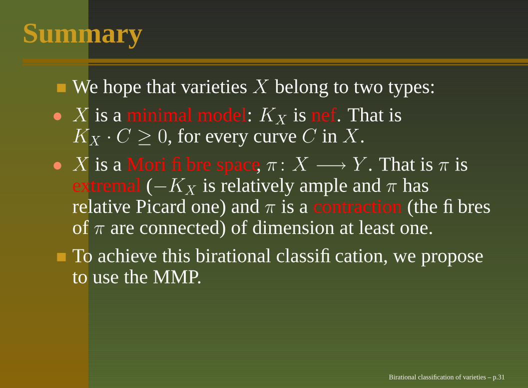
We hope that varieties X belong to two types:
• X is a minimal model: KX is nef. That isKX · C ≥ 0, for every curve C in X .
• X is a Mori fibre space, π : X −→ Y . That is π isextremal (−KX is relatively ample and π hasrelative Picard one) and π is a contraction (the fibresof π are connected) of dimension at least one.
To achieve this birational classification, we proposeto use the MMP.
Birational classification of varieties – p.31

Summary
We hope that varieties X belong to two types:
• X is a minimal model: KX is nef. That isKX · C ≥ 0, for every curve C in X .
• X is a Mori fibre space, π : X −→ Y . That is π isextremal (−KX is relatively ample and π hasrelative Picard one) and π is a contraction (the fibresof π are connected) of dimension at least one.
To achieve this birational classification, we proposeto use the MMP.
Birational classification of varieties – p.31

Two main Conjectures
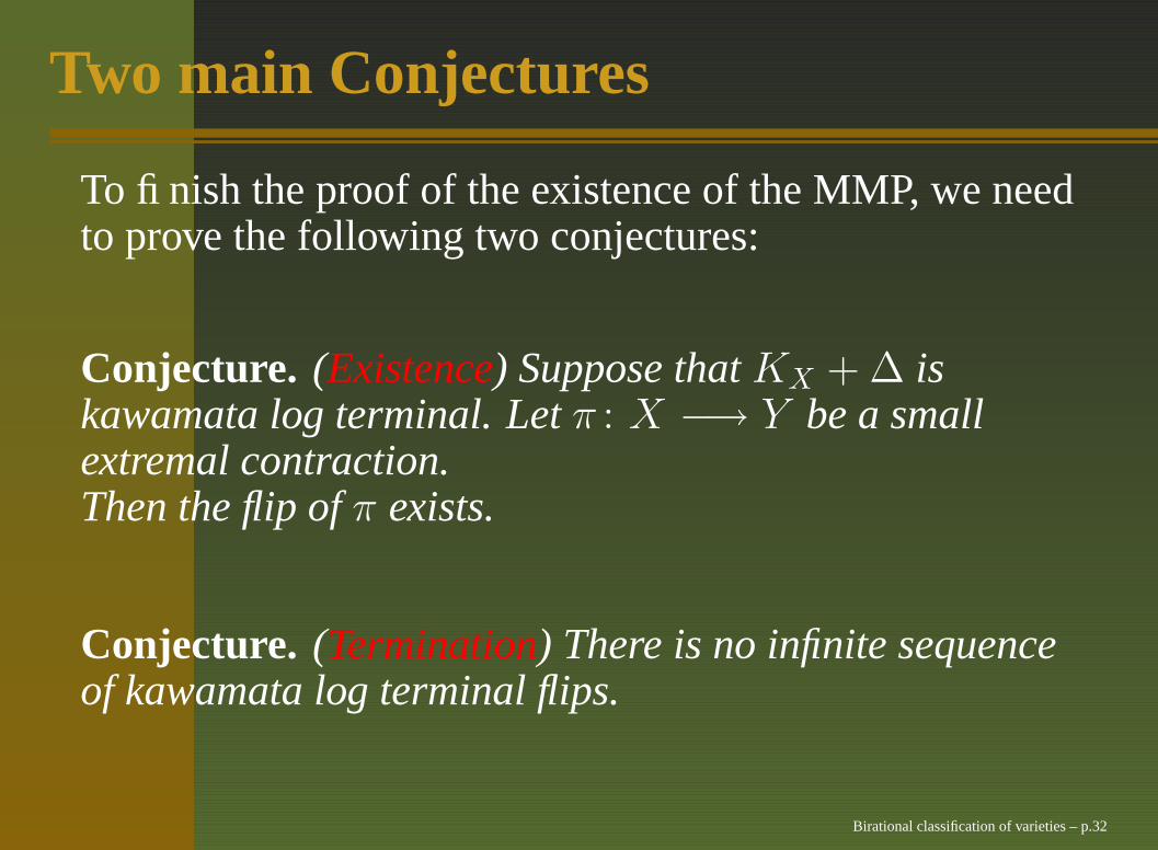
To finish the proof of the existence of the MMP, we needto prove the following two conjectures:
Conjecture. (Existence) Suppose that KX + ∆ iskawamata log terminal. Let π : X −→ Y be a smallextremal contraction.Then the flip of π exists.
Conjecture. (Termination) There is no infinite sequenceof kawamata log terminal flips.
Birational classification of varieties – p.32

Two main Conjectures
To finish the proof of the existence of the MMP, we needto prove the following two conjectures:
Conjecture. (Existence) Suppose that KX + ∆ iskawamata log terminal. Let π : X −→ Y be a smallextremal contraction.Then the flip of π exists.
Conjecture. (Termination) There is no infinite sequenceof kawamata log terminal flips.
Birational classification of varieties – p.32

Abundance
Now suppose that X is a minimal model, so that KX isnef.
Conjecture. (Abundance) Suppose that KX + ∆ iskawamata log terminal and nef.Then KX + ∆ is semiample.
Considering the resulting morphism φ : X −→ Y , werecover the Kodaira-Enriques classification of surfaces.
Birational classification of varieties – p.33