Hierarchical Aggregate Classification with Limited Supervisionfor Data Reduction in Wireless Sensor Networks∗

Lu Su Yong Yang Bolin Dinglusu2@illinois.edu yang25@illinois.edu bding3@illinois.edu

Jing Gao Tarek F. Abdelzaher Jiawei Hanjinggao3@illinois.edu zaher@illinois.edu hanj@illinois.edu

Department of Computer ScienceUniversity of Illinois at Urbana-Champaign

Urbana, IL, 61801, USA

AbstractThe main challenge of designing classification algorithms

for sensor networks is the lack of labeled sensory data, dueto the high cost of manual labeling in the harsh locales wherea sensor network is normally deployed. Moreover, deliv-ering all the sensory data to the sink would cost enormousenergy. Therefore, although some classification techniquescan deal with limited label information, they cannot be di-rectly applied to sensor networks since they are designed forcentralized databases. To address these challenges, we pro-pose a hierarchical aggregate classification (HAC) protocolwhich can reduce the amount of data sent by each node whileachieving accurate classification in the face of insufficient la-bel information. In this protocol, each sensor node locallymakes cluster analysis and forwards only its decision to theparent node. The decisions are aggregated along the tree, andeventually the global agreement is achieved at the sink node.In addition, to control the tradeoff between the communi-cation energy and the classification accuracy, we design anextended version of HAC, called the constrained hierarchicalaggregate classification (cHAC) protocol. cHAC can achievemore accurate classification results compared with HAC, atthe cost of more energy consumption. The advantages of ourschemes are demonstrated through the experiments on notonly synthetic data but also a real testbed.

∗Research reported in this paper was sponsored by NSF undergrant CNS 1040380 and by the Army Research Laboratory underCooperative Agreement Number W911NF-09-2-0053. The viewsand conclusions contained in this document are those of the authorsand should not be interpreted as representing the official policies,either expressed or implied, of the Army Research Laboratory orthe U.S. Government. The U.S. Government is authorized to repro-duce and distribute reprints for Government purposes notwithstand-ing any copyright notation here on.

Permission to make digital or hard copies of all or part of this work for personal orclassroom use is granted without fee provided that copies are not made or distributedfor profit or commercial advantage and that copies bear this notice and the full citationon the first page. To copy otherwise, to republish, to post on servers or to redistributeto lists, requires prior specific permission and/or a fee.SenSys’11, November 1–4, 2011, Seattle, WA, USA.Copyright 2011 ACM 978-1-4503-0718-5/11/11 ...$10.00

Categories and Subject DescriptorsC.2.2 [Computer-Communication Networks]: Net-

work Protocols; I.5.2 [Pattern Recognition]: DesignMethodology—Classifier design and evaluation

General TermsAlgorithms, Measurement, Experimentation

KeywordsSensor Networks, Classification, Data Reduction

1 IntroductionWireless sensor networks have been prototyped for many

military and civilian applications. Thus far, a wide spectrumof sensing devices, ranging from simple thermistors to mi-cropower impulse radars, have been integrated into existingsensor network platforms. Given the enormous amount ofdata collected by all kinds of sensing devices, techniqueswhich can intelligently analyze and process sensory datahave drawn significant attention.

Classification, which is the task of assigning objects(data) to one of several predefined categories (classes), is apervasive topic in data analysis and processing [1, 2]. Its ba-sic idea is to use a function (also called classifier) “learned”from a set of training data in which each object has featurevalues and a class label to determine the class labels of newlyarrived data. For example, consider the task of classifyingbird species based on their vocalizations. Suppose we areinterested in two bird species: Song sparrow and Americancrow, and consider two vocalization features: call intensityand call duration1. After learning from the training set, thefollowing target function can be derived: 1) low call inten-sity & short call duration → Song sparrow, and 2) high callintensity & long call duration → American crow. Supposethere is a bird with unknown species, we can judge whichclass it belongs to by mapping its feature values to the corre-sponding class based on the learnt function.

In the context of sensor networks, species recognitionlike the above example is a typical category of classifica-tion applications [3, 4, 5]. Classification also plays a keyrole in many other applications of sensor networks. In target

1We use these two features simply as an illustration, in practicebird species classification requires much more complicated featuresas in the experiment presented in Section 6.

surveillance and tracking, sensor networks should be able toclassify different types of targets, such as cars, tanks, hu-mans and animals [6, 7, 8]. In habitat monitoring, sensornetworks may distinguish different behaviors of monitoredspecies [9, 10, 11]. In environmental monitoring, it maybe desired that the environmental (e.g., weather) conditionsbe classified based on their impact on humans, animals, orcrops [12]. In health care or assisted living, an intelligentsensor network may automatically evaluate the health statusof residents, and react when they are in danger [13, 14, 15].

However, existing classification techniques designed forsensor networks fail to take into account the fact that in manyapplications of sensor networks, the amount of labeled train-ing data is usually small. The lack of labeled sensory datacan be attributed to the remote, harsh, and sometimes evenhostile locales where a sensor network is normally deployedas well as the continuous variation of the surveilled environ-ment. In such scenarios, manually creating a large trainingset becomes extremely difficult. Without sufficiently largetraining set, the learned classifier may not be able to describethe characteristics of each class, and tends to make bad pre-dictions on new data. In the area of data mining and machinelearning, some techniques called semi-supervised classifica-tion have been proposed in order to deal with insufficient la-bels [1, 2]. However, these schemes assume centralized stor-age and computation, and cannot be directly applied in thecontext of sensor networks where data are distributed over alarge number of sensors.

One possible way to apply centralized classification tech-niques is to transport all the sensory data to the sink for of-fline analysis. However, it has been revealed that wirelesstransmission of a bit can require over 1000 times more en-ergy than a single 32-bit computation [16]. Thus, in design-ing an energy-scarce sensor network, it is desired that eachnode locally process and reduce the raw data it collects asopposed to forwarding them directly to the sink [17, 18],especially for some data-intensive applications such as au-dio or video based pattern recognition. This design philoso-phy has great challenges in traditional low-end sensing plat-forms such as Mica2 mote [19]. In these platforms, sensornodes have limited processing power, memory, and energyand hence cannot support computation intensive algorithms.Recently, some powerful sensing systems [20, 21, 22, 23] arepresented, making it feasible to place the classification tasklocally on individual nodes so that communication energyand interference can be significantly reduced.

Moreover, in sensor networks, it often happens that mul-tiple sensor nodes detect the same events. Different sensornodes, due to their inaccuracy (e.g., noise in the data) andheterogeneity (e.g., different types of sensors), usually ob-serve the events from different but complementary views.Therefore, aggregating the outputs of individual nodes canoften cancel out errors and reach a much more accurate re-sult. However, aggregation of classification results is not aneasy task in the absence of sufficient labeled data due to thelack of correspondence among the outputs of different nodes.

To address the above challenges, we propose a hierarchi-cal aggregate classification (HAC for short) protocol for datareduction in sensor networks, which is built on a hierarchi-

cal tree topology where all nodes detect the same events. Inorder to overcome the obstacles presented by insufficient la-bels, we suggest that sensor nodes conduct cluster analysis,which groups data points only based on the similarity of theirfeature values without any training. The clustering resultscan provide useful constraints for the task of classificationwhen the labeled data is insufficient, since the data that havesimilar feature values are usually more likely to share thesame class label. To reduce the amount of data delivered tothe sink, we let each node locally cluster events and reportonly its clustering result (also called decision in this paper)to the parent node instead of sending the raw data which arenormally multi-dimensional numbers or audio/video files.The decisions are then aggregated along the tree through anefficient algorithm called Decision-Aggregation which canintegrate the limited label information with the clustering re-sults of multiple sensor nodes. Finally, the global consensusis reached at the sink node.

Additionally, to control the tradeoff between the commu-nication energy and the classification accuracy, we designan extended version of HAC, called the constrained hierar-chical aggregate classification (cHAC) protocol. cHAC canachieve more accurate classification results compared withHAC, at the cost of more energy consumption.

To demonstrate the advantages of our schemes, we con-duct intensive experiments on not only synthetic data but alsoa real testbed. This testbed is a good example of high-endsensing system on which various data and computation in-tensive classification applications can be deployed. In ourevaluation, we design two experiments on the testbed. Thefirst one is to classify different bird species based on theirvocalizations, and the second one is to predict the intensityof bird vocalizations as a function of different environmentalparameters measured by the sensor nodes. Both the experi-mental and simulation results show that the proposed proto-cols can achieve accurate classification in the face of insuffi-cient label information, and provide a flexible option to tunethe tradeoff between energy and accuracy.

The rest of the paper is organized as follows. Section 2introduces the general aggregation model. In Section 3, theDecision-Aggregation algorithm, which is the aggregationfunction used by the HAC and cHAC protocols at each non-leaf node, is presented. We explain how the HAC protocolutilizes this algorithm to aggregate the decisions along thetree in Section 4. In Section 5, the cHAC protocol, togetherwith the procedures it invokes, is presented. The proposedschemes are evaluated in Section 6. Then, we summarize therelated work in Section 7, and conclude the paper in Sec-tion 8.2 Aggregation Model

We consider an aggregation tree [24, 25] T rooted at thesink node (or base station), and denote the set of sensor nodeson this tree by ST = si, i = 1,2, . . . ,nT. When an eventtakes place, all the nodes collect sensory readings about it2.Let E = ei, i = 1,2, ..., t denote the sequence of events

2We assume the aggregation tree is constructed on a set of nodeswhich are deployed in proximity. Thus, they can detect the sameevents and have similar readings.

S4S3

S0

S2

S4S3

S2S1: D5=F(D1, D3, D4)S1

S0: D=F(D0, D2, D5)

(a) Aggregation Tree (b) Decision Aggregation

Figure 1. An example of decision aggregation

(sorted in chronological order) detected by the sensor nodes.Suppose only a small portion of the events are labeled, andour goal is to find out the labels of the rest events. The gen-eral idea of our solution is as follows. Based on its sensoryreadings, each node, say si, divides the events into differ-ent clusters through its local clustering algorithm. After that,si forwards the clustering result (referred to as si’s decision,denoted by Di) to its parent node. At each nonleaf node (in-cluding the sink node), the decisions of its children nodes,together with its own decision if it has one, are further ag-gregated. Figure 1 gives an illustrative example of decisionaggregation. As can be seen, the nonleaf node s1 aggregatesthe decisions of s3 and s4, together with its own decision. Inthis paper, we use function F(·) to represent the operationof decision aggregation. Then, s1 forwards the aggregateddecision D5 to the sink node s0. At s0, D5 is further com-bined with s0 and s2’s decisions. Finally, the global decisionD is obtained. In the next section, we elaborate on the de-cision aggregation operation F(·). Afterwards, we will dis-close how the HAC and cHAC protocols invoke F(·) to ag-gregate the decisions along the aggregation tree in Section 4and Section 5, respectively.

3 Decision AggregationThe decision aggregation function F(·) takes the cluster-

ing decisions of multiple sensors as well as the label infor-mation as the input, and outputs a class label for each event,indicating which class the event belongs to. Although theclustering decisions do not give the concrete label assign-ment, they provide useful information for the classificationtask. F(·) utilizes the labels from the few labeled events toguide the aggregation of clustering decisions such that a con-solidated classification solution can be finally outputted. Inthis section, we first propose to model the decision aggre-gation problem as an optimization program over a bipartitegraph. Then we present an effective solution and give per-formance analysis.

3.1 Belief GraphGiven a nonleaf node, suppose it receives n decisions

from its children nodes. In each decision, the events in E arepartitioned into m clusters3. Thus, we have totally l = mndifferent clusters, denoted by c j, j = 1,2, ..., l. In this paper,we call these clusters the input clusters (iCluster for short) of

3Most of the clustering models like K-means can control thenumber of clusters. We let the number of clusters equal the numberof classes of the events, which is m.

a decision aggregation. On the other hand, the decision ag-gregation operation will output an aggregated decision alsocomposed of m clusters, named as output clusters (oClusterfor short).

e1

Clusters

Events

Labels 21

D2

e2 e3 e4 e5 e6 e7 e8 e9

C5 C6C1 C2 C3 C4

e10

D1 D3

Figure 2. Belief graph of decision aggregation

In this paper, we represent the relationship between theevents and the iClusters as a bipartite graph, which is referredto as belief graph. In belief graph, each iCluster links to theevents it contains. Figure 2 demonstrates the belief graphof a decision aggregation. In this case, we suppose thereare t = 10 events, which belong to m = 2 different classes.Each of the sensor nodes partitions these 10 events into m = 2clusters based on its local clustering algorithm, and there aren = 3 decisions. Thus, we have totally l = mn = 6 differ-ent iClusters. Moreover, to integrate label information intothe belief graph, we add one more set of vertices, which rep-resent the labels of the events. In belief graph, the labeledevents are connected to the corresponding label vertices. Asshown in Fig. 2, event e3 and e7 are labeled, and thus linkwith label vertex 2 and 1, respectively.

3.2 TerminologyThe belief graph can be summarized by a couple of affin-

ity matrices:

• Clustering matrix A = (ai j)t×l , which links events andiClusters as follows:

ai j =

1 If ei is assigned to cluster c j.0 otherwise.

(1)

• Groundtruth matrix Zt×m = (~z1·,~z2·, . . . ,~zt·)T , which re-lates events to the label information. For a labeled eventei, its groundtruth vector is defined as:

zik =

1 If ei’s observed label is k.0 otherwise.

(2)

For each of the events without labels, we assign a zerovector~zi· =~0 to it.

Then, we define two sets of probability vectors that willwork as the variables in the optimization problem formulatedlater in the next subsection:

• For an event ei, Let Lei (i = 1,2, ..., t) denote the ID of

the oCluster to which ei is assigned, namely, the labelof ei. In our optimization problem, we aim at estimat-ing the probability of ei belonging to the k-th oCluster

(k = 1,2, ...,m), i.e., P(Lei = k|ei). Thus, each event is

associated with a m-dimensional probability vector:

~xi· = (xik)|xik = P(Lei = k|ei), k = 1,2, ...,m (3)

Putting all the vectors together, we get a probability ma-trix Xt×m = (~x1·,~x2·, . . . ,~xt·)T . After X is computed, weclassify the i-th event into the k-th class if xik attains themaximum in~xi·.

• For an iCluster c j, we also define a m-dimensional prob-ability vector :

~y j· = (y jk)|y jk = P(Lcj = k|c j), k = 1,2, ...,m (4)

where Lcj is the ID of an oCluster. In practice, P(Lc

j =k|c j) implies the probability that the majority of theevents contained in c j are assigned to the k-th oClus-ter. In theory, it will serve as an auxiliary variable in theoptimization problem. Correspondingly, the probabilitymatrix for all the iClusters is Yl×m = (~y1·,~y2·, . . . ,~yl·)T .

In our design, there is a weight parameter associated witheach decision. Initially, each decision is manually assigneda weight based on the properties (e.g., sensing capability,residual energy, location, etc) of the sensor node who makesthis decision. The weight of each node represents the im-portance of the this node, and the nodes which can providemore accurate readings are assigned higher weights. The ag-gregated decision has a weight equal to the summation of theweights of input decisions. All the clusters within a decisionhave the same weight as the decision. In the rest of this pa-per, we use w j to denote the weight of cluster c j

4. Finally,let bi = ∑m

k=1 zik be a flag variable indicating whether ei islabeled or not.3.3 Problem Formulation

With the notations defined previously, we now formulatethe decision aggregation problem as the following optimiza-tion program:

P : minX ,Y

t

∑i=1

l

∑j=1

ai jw j||~xi·−~y j·||2 +αt

∑i=1

bi||~xi·−~zi·||2 (5)

s.t. ~xi· ≥~0, |~xi·|= 1 for i = 1,2, ...,t (6)

~y j· ≥~0, |~y j·|= 1 for j = 1,2, ..., l (7)

where ||.|| and |.| denote a vector’s L2 and L1 norm respec-tively, and α is a predefined parameter. To achieve consensusamong multiple clustering decisions, we aim at finding theoptimal probability vectors of the event nodes (~xi·) and thecluster nodes (~y j·) that can minimize the disagreement overthe belief graph, and in the meanwhile, comply with the la-bel information. Specifically, the first term in the objectivefunction (Eqn. (5)) ensures that an event has similar proba-bility vector as the input cluster to which it belongs, namely,~xi· should be close to ~y j· if event ei is connected to clusterc j in the belief graph (e.g., event e3 and cluster c1, c4, c6 inFig. 2). The second term puts the constraint that a labeledevent’s probability vector ~xi· should not deviate much from

4Sometimes, we use wi to denote the weight of decision Di ornode si, and hope this causes no confusion.

Algorithm 1 Decision AggregationInput: Clustering matrix A, Groundtruth matrix Z, parameters α,set of weights W , and ε;Output: The class label for each event Le

i ;

1: Initialize Y (0), Y (1) randomly.2: τ← 13: while

√∑l

j=1 ||~y(τ)j· −~y(τ−1)

j· ||2 > ε do4: for i← 1 to t do5: ~x(τ+1)

i· = ∑lj=1 ai jw j~y

(τ)j· +αbi~zi·

∑lj=1 ai jw j+αbi

6: for j ← 1 to l do

7: ~y(τ+1)j· = ∑t

i=1 ai j~x(τ+1)i·

∑ti=1 ai j

8: τ← τ+19: for i← 1 to t do

10: return Lei ← argmaxk x(τ)

ik

the corresponding groundtruth vector~zi· (e.g., event e3 and~z3·). α can be considered as the shadow price payment forviolating this constraint. Additionally, since ~xi· and ~y j· areprobability vectors, each of their components must be greaterthan or equal to 0 and the sum should equal 1.3.4 Solution

By checking the quadratic coefficient matrix of the ob-jective function, we can show that P is a convex program,which makes it possible to find a global optimal solution.We propose to solve P using the block coordinate descentmethod [26]. The basic idea of our solution is: At the τ-thiteration, we fix the values of ~xi· or ~y j·, then the objectivefunction of P becomes a convex function with respect to ~y j·or~xi·. Therefore, its minimum with respect to~xi· and~y j· canbe obtained by setting the corresponding partial derivatives(i.e., ∂ f (X ,Y )

∂xikand ∂ f (X ,Y )

∂y jk, k = 1,2, . . . ,m) to 0:

~x(τ+1)i· =

∑lj=1 ai jw j~y

(τ)j· +αbi~zi·

∑lj=1 ai jw j +αbi

, ~y(τ+1)j· =

∑ti=1 ai j~x

(τ+1)i·

∑ti=1 ai j

(8)

The detailed steps are shown in Algorithm 1. The al-gorithm starts by initializing the probability matrix of in-put clusters randomly. The iterative process begins in line3. First, the events receive the information (i.e., ~y j·) fromneighboring clusters and update~xi· (line 5). Then, the eventspropagate the information (i.e., ~xi·) to its neighboring clus-ters to update ~y j· (line 7). Finally, an event, say ei, is as-signed to the k-th oCluster if xik is the largest probability in~xi· (line 10). According to [26] (Proposition 2.7.1), by show-ing the continuous differentiability of the objective functionand the uniqueness of the minimum when fixing ~xi· or ~y j·,we can prove that (X (τ),Y (τ)) converges to the optimal point.When solving P, we don’t take into account the constraints(Eqn. (6) and Eqn. (7)). By inductively checking the L1 normof~x(τ)

i· and~y(τ)j· from τ = 1, it can be found out that the solu-

tion obtained by Algorithm 1 automatically satisfies the con-straints.

Table 1 shows the first two iterations of the Decision-Aggregation algorithm (with α = 20 and w j = 1 for all j)for the belief graph shown in Fig. 2. We start with uniform

Table 1. Iterations of Decision AggregationY (1) X (1) Y (2) X (2)

(0.5,0.5) (0.5,0.5) (0.3913,0.6087) (0.4710,0.5290)(0.5,0.5) (0.4686,0.5314)

(0.5,0.5)(0.0652,0.9348)

(0.5725,0.4275)(0.0536,0.9464)

(0.5,0.5) (0.4710,0.5290)(0.5,0.5)

(0.5,0.5)(0.5870,0.4130)

(0.4710,0.5290)(0.5,0.5) (0.5290,0.4710)

(0.5,0.5)(0.9348,0.0652)

(0.4130,0.5870)(0.9464,0.0536)

(0.5,0.5) (0.5314,0.4686)(0.5,0.5)

(0.5,0.5)(0.6087,0.3913)

(0.5290,0.4710)(0.5,0.5) (0.5,0.5) (0.4275,0.5725) (0.5290,0.4710)

probability vectors for the six clusters (Y (1)). Then the prob-abilities of the events without labels are calculated by aver-aging the probabilities of the clusters they link to. At thisstep, they all have (0.5, 0.5) as their probability vectors. Onthe other hand, if the event is labeled (e.g., e3 and e7 in thisexample), the labeled information is incorporated into theprobability vector computation where we average the prob-ability vectors of the clusters each event links to and that ofthe groundtruth label (note that the vote from the true labelhas a weight α). For example, e3 is adjacent to c1, c4, c6 andlabel 2, so we have ~x (1)

3· = (0.5,0.5)+(0.5,0.5)+(0.5,0.5)+α·(0,1)3+α =

(0.0652,0.9348). During the second iteration, ~y (2)j· is ob-

tained by averaging the probabilities of the events it contains.For example, ~y (2)

1· is the average of ~x (2)2· , ~x (2)

3· , ~x (2)5· and ~y (2)

9· ,which leads to (0.3913,0.6087). The propagation continuesuntil convergence.

3.5 Performance AnalysisIt can be seen that at each iteration, the algorithm takes

O(tlm) = O(tnm2) time to compute the probability vectorsof clusters and events. Also, the convergence rate of coor-dinate descent method is usually linear [26] (in practice, wefix the iteration number as a constant). Thus, the computa-tional complexity of Algorithm 1 is actually linear with re-spect to the number of events (i.e., t), considering that thenumber of nodes involved in each aggregation (i.e., n) andthe number of classes (i.e., m) are usually small. Thus, theproposed algorithm is not more expensive than the classi-fication/clustering schemes, and thus can be applied to anyplatform running classification tasks. Furthermore, sincewireless communication is the dominating factor of the en-ergy consumption in sensor networks, our algorithm actuallysaves much more energy than it consumes.

4 Hierarchical Aggregate ClassificationHere we introduce the Hierarchical Aggregate Clas-

sification (HAC) protocol. HAC applies the Decision-Aggregation algorithm on each of the nonleaf nodes to ag-gregate all the decisions it collects. The output of the algo-rithm, i.e., the aggregated decision is forwarded upwards bythe nonleaf node, and serves as one of the input decisions inthe aggregation at its parent node. The message carrying thedecision consists of t entries, corresponding to t events. Ineach entry, the index of an event and the ID of the oCluster towhich this event belongs are stored. As previously defined,the ID of each oCluster is the label of this oCluster. How-

ever, these labels may not be useful in later aggregations,because the oClusters will probably be combined with otherclusters whose labels are unknown. For instance, at the sinks0 shown in Fig. 1(b), the labeled clusters in decision D5 arecombined with unlabeled clusters in D0 and D2. Finally, theglobal decision is obtained at the sink node, and each eventis assigned a predefined label.

5 Constrained Hierarchical Aggregate Classi-fication

In this section, we introduce an extended version of theHAC protocol, called the Constrained Hierarchical Aggre-gate Classification (cHAC) protocol. cHAC also uses theDecision-Aggregation algorithm as the aggregation function.However, different from HAC which requires that each non-leaf node aggregates all the decisions it collects, cHAC intel-ligently plans the decision aggregations throughout the treesuch that more accurate classification results can be obtainedat the cost of more energy consumption. In the rest of thissection, we first use a simple example to illustrate how en-ergy and accuracy are correlated during the process of deci-sion aggregation. Then we present the cHAC protocol, to-gether with the procedures it invokes. Finally, the perfor-mance of cHAC is analyzed.

5.1 Tradeoff between Energy and AccuracyHierarchical aggregate classification, as discussed in the

previous sections, can improve the classification accuracy aswell as the consumption of communication energy throughcombining decisions coming from different sensor nodes.However, decision information is inevitably lost during theprocess of aggregation, and this may hurt the accuracy of theaggregated decision.

S4S3

1

S2

1

1

1

S1: V(1, 1, 0)=1

S0: V(3×1, 0, 0)=1

(a)

S4S3

1

S2

3

1

1

S1: 1, 1, 0

S0: V(1, 1, 0, 0, 0)=0

(b)

S4S3

1

S2

2

1

1

S1: V(1, 1)=1, 0

S0: V(2×1, 0, 0, 0)=0

(c)

Figure 3. An example of energy-accuracy tradeoff

Let’s continue to study the example shown in Fig. 1. Sup-pose all of the five sensors detect an event and try to pre-dict the label of this event. To simplify the explanation,in this case we assume the sensor nodes are doing classi-fication (not clustering). There are two classes with label0 and 1 respectively. The local decisions of the nodes are:D0 = D1 = D2 = 0 and D3 = D4 = 1 (recall that Di is si’sdecision). Here we use a simple method, i.e., majority vot-ing, as the aggregation function (denoted by V(·)). Note thatonly in this example we use majority voting as the aggre-gation function, in every other part of this paper, the aggre-gation function means the Decision-Aggregation algorithm.Intuitively, given that the weight of each node is 1, the ag-gregated result of all the decisions should be 0, since thereare more 0s than 1s among the 5 atomic decisions.

Figure. 3(a) illustrates the process of hierarchical aggre-gate classification along the aggregation tree, where the num-bers on the links imply the number of decisions transmittedalong this link. At node s1, D1, D3 and D4 are combined. Theresultant decision, which is D5, is evaluated to be 1, sincethe majority of input decisions (D3 and D4) choose label 1.Then, D5 is sent to the sink s0, where the final aggregationhappens. Since D5 is the combination of three atomic deci-sions, its weight is the aggregate weight of three nodes, i.e.,w5 = 3. Therefore, the final aggregation is calculated as fol-lows: V(w5D5,w0D0,w2D2) = V(3× 1,0,0) = 1. Clearly,this result is not accurate, since more than half of the nodespredict the label of the event to be 0. The problem lies in theaggregation at node s1, where some decision information,i.e., D1 = 0 is lost5.

5.2 Problem FormulationTo address this problem, we propose to trade energy for

accuracy. Specifically, we add a constraint to the hierarchicalaggregate classification, namely, in each decision aggrega-tion along the tree (including the aggregation at the sink), theweight of each input decision cannot be larger than a prede-fined percentage of the total weight of all this aggregation’sinput decisions. Formally, suppose D is the set of the in-put decisions involved in an aggregation (note that D is NOTthe set of all nodes’ decisions), then it must be satisfied that

wi∑Dk∈D wk

≤ δ for ∀ Di ∈D , where wi (wk) denotes the weight

of decision Di (Dk), and δ is a predefined percentage. Inthis paper, we call δ the weight balance threshold, and theconstraint defined above the weight balance constraint. Theweight balance threshold δ is a control parameter which cantune the tradeoff between energy and accuracy.

Intuitively, the smaller δ is, the larger number of decisionsare combined in each aggregation, and thus the aggregateddecision is closer to the global consensus. For example, ifall the sensor nodes have the same weight and δ = 1

n (n isthe total number of sensor nodes), the weight balance con-straint requires that each combination takes at least n deci-sions, which indicates that all the decisions need to be sentto the sink node without any aggregation on the half way.Clearly, the result of this aggregation perfectly represents theglobal consensus. Moreover, when δ is small, to guaranteethat a large number of decisions are combined in each ag-gregation, some decisions have to be transmitted for morethan one hop along the aggregation tree, resulting in moretransmissions.

For the simplicity of presentation, we assume that in eachtransmission, only one decision is forwarded. We are inter-ested in the problem of Constrained Hierarchical AggregateClassification: Under the weight balance constraint, among

5Note that in this simple example, s1 can send the numbers of 1sand 0s picked by its children (together with itself) to achieve betterconsensus compared with sending the majority voting result only.However, this solution cannot work for the decision aggregationproblem where only clustering results are available. Since the samecluster ID may represent different classes in different decisions, wecannot simply count the number of labels assigned by the decisions.Furthermore, when the number of classes is large, this solution willconsume excessive energy.

all the legal ways (solutions) which can aggregate the atomicdecisions along the aggregation tree to reach a consensusat the sink, we want to pick the one with the minimum to-tal number of transmissions. In fact, the hierarchical aggre-gate classification problem discussed in previous sections isequivalent to the case when δ = 1.

Let’s get back to the example shown in Fig. 3. Suppose inthis case, δ is set to be 0.5. Apparently, the aforementionedsolution (Fig. 3(a)) does not satisfy this constraint, since theweight percentage of D5 in the final aggregation is more thanhalf. Thus, although the absolute minimum transmissionnumber (which is 4) is achieved in this case, it is not a validsolution. In contrast, a feasible solution is shown in Fig. 3(b).In this scenario, node s1 does not make any aggregation, butdirectly forwards the decisions (D1=0, D3=1 and D4=1) tothe sink. This will surely satisfy the balance constraint. Inaddition, this solution actually achieves the highest accuracy,since no information is lost before arriving at the sink node.However, it results in unnecessary energy consumption (6transmissions in total). Finally, Fig. 3(c) shows the opti-mal solution. Specifically, node s1 combines two out of thethree decisions (D5 = V(D3,D4) = V(1,1) = 1), and deliv-ers the resultant decisions (D1 and D5) to the sink through2 transmissions. This solution spends 5 transmissions, theminimum energy consumption that can be achieved underthe weight balance constraint. More importantly, the globaldecision achieved by this solution is 0, which correctly rep-resents the majority of the nodes.

As a matter of fact, the constrained hierarchical aggregateclassification (cHAC) problem is an NP-complete problem.We prove this proposition by the following theorem:Theorem 1. The constrained hierarchical aggregate classi-fication problem is NP-complete.PROOF. First of all, we restate the cHAC problem as a de-cision problem. That is, we wish to determine whether thedecision aggregation along a given tree can be done at thecost of exactly k transmissions. In this proof, we will showthat the equal-size partition problem (ePartition for short), aknown NP-complete problem, can be reduced to cHAC, i.e.,ePartition ≤P cHAC. The equal-size partition problem is todecide whether a given set of integers can be partitioned intotwo “halves” that have both the same size (number of inte-gers) and the same sum (summation of the integers).

The reduction algorithm begins with an instance of ePar-tition. Let A = a1,a2, · · · ,an (n ≥ 8) be a set of integers.We shall construct an instance of cHAC (denoted by Φ) suchthat A can be equally partitioned if and only if the answer toΦ is yes.

S0

?

SnS1 S2

11 1

S0

2

SnS1 S2

11 1

Sn+1: F(BS), F(CS)

(a) (b)

Sn+1

Figure 4. NP-completeness of cHAC

Φ is constructed as follows. An aggregation tree is shownin Fig. 4(a). The root node s0 has a single child, which issn+1. There are n nodes (s1,s2, · · · ,sn) connected to sn+1.Suppose the weight of node si, i = 1,2, · · · ,n is ai + M,where M is a very large positive integer. Moreover, theweights of s0 and sn+1 are ∑n

i=1 ai+nM2 and 0, respectively. In

this case, the weight balance threshold is set to be δ = 13 .

Then, we introduce the formal description of Φ: Is therea way to solve the cHAC problem on the tree shown inFig. 4(a) such that the total number of transmissions is ex-actly n+2.

Suppose A can be partitioned into two equal-size sub-sets with equal summation. We denote these two subsetsby B and C . Without loss of generality, we suppose B =a1,a2, · · · ,a n

2 and C = a n

2 +1,a n2 +2, · · · ,an, and thus we

have ∑n2i=1 ai = ∑n

j= n2 +1 a j. Correspondingly, we put nodes

s1,s2, · · · ,s n2

in BS and s n2 +1,s n

2 +2, · · · ,sn in CS (as shownin Fig. 4(b)). Since wi = ai + M, it can be derived that

∑n2i=1 wi = ∑n

j= n2 +1 w j, namely, BS and CS have the same to-

tal weight. In addition, no elements in BS and CS violatethe weight balance constraint given that M is a large inte-ger. Then, we combine decisions in BS and CS at node sn+1,and use 2 transmissions to send the combined ones to sn+1.Furthermore, since the weight of each combined decision is∑n

i=1 ai+nM2 , which equals s0’s weight, the three decision (two

combined decisions and s0’s decision) can be aggregated atnode s0 without violating the weight balance constraint (re-call that δ = 1

3 ). Furthermore, since n transmissions areneeded to move the clustering decision of each leaf node tonode sn+1, altogether n+2 transmissions are used during thisprocess, and thus the answer to Φ is yes.

Conversely, suppose the answer to Φ is yes. Since n trans-missions (from si to sn+1) are inevitable, we have to use 2transmissions to send decisions from sn+1 to s0. It is easy tosee that the only way to achieve this is to combine the deci-sions at sn+1 into BS and CS with the same weight ∑n

i=1 ai+nM2 ,

and then send them to s0. For M is large, BS and CS musthave the same size, and thus the corresponding halves B andC in A also have the same sum ∑n

i=1 ai2 (and of course, the

same size). So Φ is yes implies that the ePartition instance isyes.

In summary, ePartition ≤P cHAC is proved, and thuscHAC is NP-hard. Furthermore, it is straightforward to showthat cHAC∈ NP, and thus a conclusion can be drawn thatcHAC is NP-complete.

The NP-completeness of the constrained decision aggre-gation problem makes it hopeless to find the optimal solutionin polynomial time. In the rest of this section, we’ll introducean approximate solution, which is proved to have a constantapproximation ratio and a polynomial complexity.5.3 Constrained Decision Aggregation

In this subsection, we introduce the key function of oursolution, which is called constrained decision aggregation.The constrained decision aggregation procedure works ateach nonleaf tree node, except the sink. It partitions the de-cisions gathered at this node into different sets and invokes

Decision-Aggregation to combine the decision sets which re-spect the weight balance constraint.

Intuitively, to guarantee that the final decision aggregationat the sink node is legal, each decision arriving at the sinkshould have a weight smaller than or equal to W = bδWT c(where WT denotes the total weight of all the sensor nodeson the aggregation tree). Therefore, at any nonleaf node ex-cept the sink, the summation of the weights of all the inputdecisions involved in any aggregation must not exceed W .This is an additional constraint called the weight summationconstraint for each nonleaf node. Also, W is referred to asthe weight summation threshold. From the analysis above, itis easy to see that any solution to the constrained hierarchicalaggregate classification problem satisfies this constraint.

Consequently, at each nonleaf node, before aggregate thedecisions, we need to solve the following problem first: Con-sider a nonleaf node s0 with n children nodes si, i = 1,2, ...,n.The goal is to divide the decision set D = D1,D2, ...,Dninto the minimum number of subsets such that each multi-decision subset respects both the weight summation con-straint and the weight balance constraint. Since node s0spends one transmission to forward each aggregated subsetor single-decision subset to its parent, minimizing the sub-set number implies the minimization of transmission num-ber. To solve this problem, we introduce Decision-Selection,an algorithm which can pick a valid subset of decisions aslong as there exists one. Afterwards, we give a formal def-inition of the Constrained-Decision-Aggregation procedurewhich iteratively invokes Decision-Selection and Decision-Aggregation to select and combine the decisions.

Decision-Selection is a dynamic programming based ap-proach. First of all, we define a couple of notations. (a)V [i,w]: V [i,w] = 1 if out of the first i decisions in D , it ispossible to find a subset in which the aggregate weight ofall the decisions is exactly w, and V [i,w] = 0 otherwise. (b)keep[i,w]: keep[i,w] = 1 if decision Di is picked in the subsetwhose total weight is w, and keep[i,w] = 0 otherwise. Theinitial settings of V [i,w] are described as below:

V [0,w] = 0 for 0≤ w≤W (9)V [i,w] =−∞ for w < 0 (10)V [i,wi] = 1 for 1≤ i≤ n (11)

In Decision-Selection, V [i,w] is recursively calculatedbased on Eqn. (12) for 1≤ i≤ n and 0≤ w≤W .

V [i,w] = max(V [i−1,w],V [i−1,w−wi]) (12)

Algorithm 2 describes the detailed steps of Decision-Selection. Given a particular decision Di and a weight sumw, what we are concerned about is under which condition Dicould be selected to the output decision set (i.e., set keep[i,w]to be 1), which can not be directly seen from Eqn. (12).There are two possible cases. Case 1 happens in line 8. Inthis case, among the first i−1 decisions, we can find a subsetwith total weight w−wi (i.e., V [i−1,w−wi] = 1), but cannotfind a subset with total weight w (i.e., V [i−1,w] = 0). Obvi-ously, Di should be selected; Case 2 is in line 12. In this case,

Algorithm 2 Decision SelectionInput: Weight summation threshold W , set of weights W , set ofinput decisions D , weight balance threshold δ;Output: Set of decisions A satisfying both weight summation con-straint and weight balance constraint;1: A ←Φ2: for w← 0 to W do3: V [0,w]← 0;4: for i← 1 to n do5: for w← 0 to W do6: if wi < w and V [i−1,w−wi] > V [i−1,w] then7: V [i,w]←V [i−1,w−wi];8: keep[i,w]← 1;9: else if wi = w then

10: V [i,w]← 1;11: if V [i−1,w] = 0 then12: keep[i,w]← 1;13: else14: keep[i,w]← 0;15: else16: V [i,w]←V [i−1,w];17: keep[i,w]← 0;18: for w←W downto 1 do19: m← w;20: for i← n downto 1 do21: if keep[i,m] = 1 and wi ≤ bδwc then22: A ← A

⋃Di;23: m← m−wi;24: if A 6= Φ then25: break;26: return A

though w = wi, we put Di into the selected set only when nosubset among the first i− 1 decisions has a total weight ofw (i.e., V [i− 1,w] = 0), since the algorithm only picks oneset for a particular weight sum. Decision-Selection has animportant prerequisite: D must be sorted in the ascendingorder of weight. The motivation of this prerequisite can bebetter understood via Theorem 2.Theorem 2. Decision-Selection can return a valid decisionset satisfying both the weight summation constraint and theweight balance constraint, as long as there exists such a setin D .PROOF. There is no doubt that given a number 1 < w < W ,Algorithm 2 can identify a subset of D whose weight sum-mation is exactly equal to w, if such a subset really exists.There are at most W subsets found by the algorithm (storedin keep[i,w]), and all of them satisfy the weight summa-tion constraint. Thus, we only need to show that if none ofthese selected subsets can satisfy the weight balance con-straint, there does not exist a legal decision subset in D .The key point is, given a weight summation w, there mayexist multiple valid subsets, and among them, the subset(denoted by D∗(w)) whose last decision has the smallestweight is the most likely to satisfy the weight balance con-straint. This is because the decisions are sorted in the as-cending order of the weight. Thus, given a decision set, ifthe last decision, which has the largest weight, satisfies theconstraint, all the preceding decisions in this set satisfy theconstraint as well. The Decision-Selection algorithm guar-

Algorithm 3 Constrained Decision AggregationInput: Set of input decisions DOutput: Set of output decisions Ω1: Sort D in the ascending order of weight;2: repeat3: A ← Decision-Selection(D);4: D ←D−A ;5: C ← C

⋃Decision-Aggregation(A);6: until |A |= 07: R ←D;8: Ω← C

⋃R ;

9: return Ω

antees to pick D∗(w), since a decision Di is selected (i.e.,keep[i,w] ← 1, line 8 and 12) only when no valid subsetexists among the first i− 1 decisions (i.e., V [i− 1,w] = 0,line 6 and 11). For example, suppose we have a sorted de-cision set D = w1 = 2,w2 = 3,w3 = 4,w4 = 7, with theweight sum w = 9 and the balance threshold δ = 1

2 . It isobvious that there are two subsets of D whose weight sumequals w. They are D1 = 2,3,4 and D2 = 2,7. Amongthem, only D1, whose last decision has a smaller weight,can satisfy the weight balance constraint. In the algorithm,keep[3,9] will be set by 1, and keep[4,9] is assigned to be0 since V [3,9] = 1. Finally, lines 18-25 exhaustively checkD∗(w) (line 21) with w ranging from W down to 1, and thuswill not miss a valid subset if it does exist.

With Decision-Selection, we are able to design theConstrained-Decision-Aggregation algorithm. As shownin Algorithm 3, after sorting D in the ascending orderof weight, Constrained-Decision-Aggregation iteratively in-vokes Decision-Selection (line 3), and combines the returneddecision set (i.e., A) through the procedure of Decision-Aggregation (line 5). The resultant aggregated decisions arestored in a set C . This process repeats until no more set isfound by Decision-Selection, then the residual decisions leftin D are moved to another set R . In line 8, the union of Cand R forms the set of output decisions Ω. Finally, |Ω| trans-missions are consumed by the subtree root s0 to forward theoutput decisions in Ω to its parent node.

5.4 Constrained Hierarchical Aggregate Clas-sification

The constrained hierarchical aggregate classification(cHAC) protocol invokes the Constrained-Decision-Aggregation procedure at each nonleaf node except the sink,and aggregates the decisions along the tree. Specifically,suppose n subtrees are connected to a nonleaf node s0.cHAC applies Constrained-Decision-Aggregation to eachof the subtrees Ti, resulting in a set of aggregated decisionsCi and a set of residual decisions Ri. After arriving at s0,these sets form two union sets, which are C0 =

⋃ni=1 Ci and

R0 =⋃n

i=1 Ri. Then, cHAC employs Constrained-Decision-Aggregation on R0, and puts the newly aggregated decisionsin C0. After the algorithm terminates, no decisions leftin R0 can be further combined. Subsequently, s0 spends|Ω0| = |C0|+ |R0| transmissions to forward the decisions.Altogether, ∑n

i=0 |Ωi| transmissions are consumed duringthis process. In each transmission, the cHAC protocol uses

the same message format as the HAC protocol to carry thedecision.

At the sink node, the procedure of Decision-Aggregation(not Constrained-Decision-Aggregation) is called, sincenone of the arrived decisions has a weight larger than W =bδWT c. Finally, the global consensus is achieved. It is easyto see, the cHAC protocol can be easily implemented in adistributed manner. Each node only needs to collect the de-cision information from its children and make local aggrega-tions. Therefore, no global coordination is needed.5.5 Performance Analysis

In this subsection, we show the approximation ra-tio and the computational complexity of not only theConstrained-Decision-Aggregation algorithm but also thewhole constrained hierarchical aggregate classification pro-cess. We start with the analysis of the Constrained-Decision-Aggregation algorithm. First of all, we have the followingobservation.Lemma 1. After Constrained-Decision-Aggregation termi-nates, there are at most one decision in C whose weight is nomore than W

2 .The basic idea of the proof is: suppose there are two

such decisions, they are resulted from two decision subsetswhose weight summation is no more than W

2 . However, theDecision-Selection algorithm should have combined thesetwo subsets into one which satisfies both the weight balanceconstraint and the weight summation constraint. In fact, ifthere exists a decision in C with a weight less than or equalto W

2 , we move it from C to R .

2 3

Figure 5. Intervals

According to Algorithm 3, the residual set R contains thedecisions that cannot be aggregated. We project these deci-sions onto an interval [1,W ] based on their weights. Then,we divide the interval [1,W ] into subintervals by the points2i, i = 1,2, ...,blog2(δW/2)c (together with the point δW/2),as shown in Fig. 5. Before proving the approximation ratioof Constrained-Decision-Aggregation in Theorem 3, we firstprove the following claim in Lemma 2.Lemma 2. Within each interval, there are less than 2

δ deci-sions in R .PROOF. By contradiction, suppose there are 2

δ decisionswithin an interval delimited by the point 2i−1 and 2i. Thesum of their weights is less than W , for i ≤ blog2(δW/2)c.Within [2i−1,2i], the aggregate weight of these decisions isat least 2

δ ·2i−1 = 2i

δ , while the weight of a single decision isat most 2i. Thus, the weight percentage of any decision inthis interval is at most δ, which satisfies the weight balanceconstraint. This contradicts with the fact that Constrained-Decision-Aggregation leaves them uncombined, so the proofis completed.Theorem 3. Suppose OPT is the transmission number inthe optimal solution to the constrained decision aggregationproblem, and SOL is the transmission number in the solution

found by the Constrained-Decision-Aggregation algorithm.We have SOL≤ 2

δ ·(

OPT+ log2δW2

).

PROOF. First of all, we define some notations. Let WD de-note the total weight of the decisions in D . In addition, R≤and R> are two subsets of R in which the weights of de-cisions are smaller than or equal to δW/2 and larger thanδW/2, respectively. An lower bound of OPT is WD/W ,since every (aggregated) decision has a weight of at mostW . In our algorithm, decisions in D are partitioned andaggregated into two sets C and R , and we have SOL =|C |+ |R | = |C |+ |R≤|+ |R>|. For all the decisions in Cwhose weights are at least W/2 and all the decision in R>

whose weights are at least δW/2, we have |C |+ |R>| ≤WD

δW/2 = 2δ ·

WDW ≤ 2

δ ·OPT, for OPT ≥WD/W . In addition,

by Lemma 2, we have |R≤| ≤ 2δ · log2

δW2 . Thus, combin-

ing the above two inequalities, we can derive the promisedbound SOL≤ 2

δ ·(

OPT+ log2δW2

).

Then, the computational complexity of Constrained-Decision-Aggregation is given by Theorem 4.Theorem 4. Constrained-Decision-Aggregation has a com-putational complexity of O(n2δW )6.PROOF. First of all, Constrained-Decision-Aggregationsorts the decisions in D , which takes a running time ofO(n logn). Then, in the loop between line 2 and 6, Decision-Selection is repeatedly called, and each takes O(nW ). Sinceunder the weight balance constraint, the number of decisionspicked by Decision-Selection in each iteration must be noless than 1

δ , the number of times that Decision-Selection iscalled is at most δn. Therefore, the overall computationalcomplexity of the Constrained-Decision-Aggregation proce-dure is O(n log(n))+δnO(nW ) = O(n2δW ).

Next, we give the approximation ratio and the computa-tional complexity of the whole constrained hierarchical ag-gregate classification process by Theorem 5 and Theorem 6,respectively.Theorem 5. Suppose OPT is the transmission number inthe optimal solution to the constrained hierarchical aggregateclassification problem, and SOL is the transmission numberin the solution found by the cHAC protocol. Then, we haveSOL≤ 2

δ ·(

1+ log2δW2

)·OPT.

PROOF. The proof is similar to the proof of Theorem 3in spirit, but the bound we derived is a bit weaker. Sup-pose the tree has n nodes (excluding the sink node). LetOPT = OPT1 +OPT2 + . . .+OPTn, where OPTi is the num-ber of transmissions from node si to its parent in the opti-mal solution. Similarly, SOL = SOL1 +SOL2 + . . .+SOLn,where SOLi is the number of transmissions from si to its par-ent in the solution obtained by the cHAC protocol.

In case that si is a nonleaf node, the cHAC protocoltakes the aggregated decisions from its children as the in-put. Intuitively, the lower bound of OPTi is the optimalsolution (denoted by OPTi) to the problem that takes allthe atomic decisions without being aggregated as the in-put. Thus, similar to the analysis in Theorem 3, we have

6In this analysis, we do not consider Decision-Aggregation,since it can be decoupled from Constrained-Decision-Aggregation.

SOLi ≤ 2δ ·

(OPTi + log2

δW2

)≤ 2

δ ·(

1+ log2δW2

)· OPTi. If

si is a leaf node, it is apparent that SOLi = OPTi. SinceOPTi ≤ OPTi, summing them up for i = 1,2, . . . ,n, we canderive the promised bound SOL≤ 2

δ ·(

1+ log2δW2

)·OPT≤

2δ ·

(1+ log2

δW2

)·OPT.

Theorem 6. The cHAC protocol has a computational com-plexity of O(n2

TW ).Recall that here nT denotes the total number of nodes

on the aggregation tree. In the worst case, the Decision-Selection algorithm is called for O(nT ) times, and each takesO(nTW ) time. Therefore, the overall computational com-plexity of the cHAC protocol is O(n2

TW ).

6 Performance EvaluationIn this section, we evaluate the proposed schemes on

i) Synthetic data, and ii) A solar-powered sensor networktestbed. For comparison, we design two baseline methods.Both of the baselines adopt the strategy of majority-voting,and they are different in the ways of generating votes. Thefirst baseline method, which we call Clustering Voting, sug-gests that each node locally groups the events into differ-ent clusters (this part is the same as our scheme), and thencount the labeled events (i.e., how many events belong toa particular label) in each cluster. Within a cluster, all theevents are assigned the label with the largest count. For ex-ample, suppose there are totally 100 events in a cluster, withthree events labeled 1 and two events labeled 0, then all the100 events are labeled 1 according to the clustering votingscheme. Finally, the nodes vote to decide the label of eachevent. The second baseline, called Classification Voting, letseach node apply classification algorithms (such as decisiontree, SVM) on the labeled data, and predict the labels of therest. Then, the events are labeled based on the vote. Thedetailed experimental results are shown and explained in thenext two subsections.

6.1 Experiment on Synthetic DataIn this part, we evaluate our schemes on synthetic data.

First of all, we randomly build aggregation trees with thenumber of tree nodes ranging from 20 to 80. The height ofthe trees increases with the augment of tree size. In particu-lar, the trees of height 3, 4, 5 and 6 contain around 20, 30, 50and 80 nodes, correspondingly. In order to achieve diversity,we apply different clustering algorithms (such as K-means,spectral clustering) to different nodes. Suppose each nodehas a weight between 0 and 5. For each height, we evaluatedifferent tree topologies and record the average results.

Next, we give a brief description on how the syntheticdata is generated. In this experiment, we assume there are10 different types of sensors, corresponding to 10 featuresof the events (e.g., temperature, humidity, etc). Suppose theevents are drawn from 5 different classes (labels), and werandomly assign the groundtruth labels (from 5 classes) to10000 events. For each event, based on its assigned label,we generate its feature values from a Gaussian distributionin a 10-dimensional (each dimension corresponds to a fea-ture) data space R10. Therefore, the collection of the eventsare drawn from a Gaussian mixture model with 5 compo-

1 2 3 4 5 6 7 8 9 1060

65

70

75

80

85

90

95

Label Percentage

Acc

urac

y

HACcHAC, δ=1/2cHAC, δ=1/3Clustering VotingClassification Voting

Figure 6. Comparison of accuracy (Synthetic data)

nents, each of which corresponds to a class. After creatingthe events, we generate the sensory readings of the nodes.For each node on the tree, we randomly assign a subset of thepreviously defined (10 types of) sensors to it. For each typeof sensor assigned to this node, we generate its sensory read-ing of each event as follows: we first copy the correspond-ing feature value of the event and then add random Gaussiannoise to this value. In this way, different nodes with the sametypes of sensors would have different sensory readings.

1 1/2 1/3 1/4 1/5 1/6 1/7 1/8 1/90

100

200

300

400

δ

Ene

rgy

Height=3Height=4Height=5Height=6

1 1/2 1/3 1/4 1/5 1/6 1/7 1/8 1/975

80

85

90

95

100

δ

Acc

urac

y

Height=3Height=4Height=5Height=6

(a) δ on energy (b) δ on accuracyFigure 7. Impact of δ on energy and accuracy (Synthetic data)

Figure 6 compares the classification accuracy (percent-age of the correctly classified events) of the proposed hierar-chical aggregate classification (HAC) and constrained hierar-chical aggregate classification (cHAC) (with weight balancethreshold δ = 1/2, 1/3, and 1/4, respectively) protocols, andthe two baseline schemes. As can be seen, when the percent-age of labeled events is less than 10, the proposed protocolscan always achieve better performance than the baselines.Moreover, with the decrease of label percentage, the accu-racy of all the five methods degrade. Among them, the accu-racy of the classification voting decreases the fastest. This isreasonable since compared with clustering methods, classi-fication models are normally more sensitive to the label per-centage. Another notable point is that the cHAC with smallerδ can achieve higher accuracy.

Figure 7 demonstrates the impact of weight balancethreshold δ on the communication energy (in terms of thetotal number of messages transmitted by the tree nodes) andthe classification accuracy of the cHAC protocol. In this ex-periment, we assume 5% of the events are labeled, and testfour groups of aggregation trees, with height 3, 4, 5 and 6respectively. As expected, when δ decreases, no matter ofthe tree size, more energy is consumed (Figure 7(a)), andhigher accuracy can be achieved (Figure 7(b)). This con-

SSolar Panels

N d E lNode Enclosure

Figure 8. Outside look of a solar-powered sensor node

Waterproof enclosure

ComputerWireless

RouterBattery

Figure 9. Inside look of a solar-powered sensor node

Air Pressure Sensor Camera

Wind Sensor Tmote MicrophoneWind Sensor Tmote Microphone

Figure 10. Different types of sensorson the nodes

firms our scheme’s capability of trading energy for accuracy.Furthermore, given a δ, the trees with larger height tend tohave higher accuracy, however, at the cost of more energyconsumption. This is because usually better diversity canbe obtained when more nodes are involved in the aggrega-tion. Finally, when δ becomes lower than a threshold (e.g.,δ = 1

5 for height-3 trees), the accuracy cannot be improvedany more, since all the atomic decisions (locally made byeach node) have been sent to the sink.

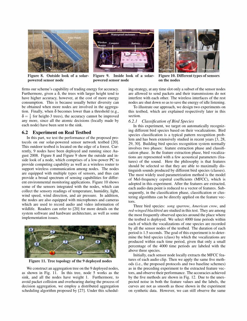
6.2 Experiment on Real TestbedIn this part, we test the performance of the proposed pro-

tocols on our solar-powered sensor network testbed [20].This outdoor testbed is located on the edge of a forest. Cur-rently, 9 nodes have been deployed and running since Au-gust 2008. Figure 8 and Figure 9 show the outside and in-side look of a node, which comprises of a low-power PC toprovide computing capability as well as a wireless router tosupport wireless communication among nodes. The nodesare equipped with multiple types of sensors, and thus canprovide a broad spectrum of sensing capabilities for differ-ent environmental monitoring applications. Figure 10 showssome of the sensors integrated with the nodes, which cancollect the sensory readings of temperature, humidity, light,wind speed, wind direction, and air pressure. In addition,the nodes are also equipped with microphones and cameraswhich are used to record audio and video information ofwildlife. Readers can refer to [20] for more details on thesystem software and hardware architecture, as well as someimplementation issues.

Figure 11. Tree topology of the 9 deployed nodes

We construct an aggregation tree on the 9 deployed nodes,as shown in Fig. 11. In this tree, node 5 works as thesink, and all the nodes have weight 1. Furthermore, toavoid packet collision and overhearing during the process ofdecision aggregation, we employ a distributed aggregationscheduling algorithm proposed by [27]. Under this schedul-

ing strategy, at any time slot only a subset of the sensor nodesare allowed to send packets and their transmissions do notinterfere with each other. The wireless interfaces of the restnodes are shut down so as to save the energy of idle listening.

To illustrate our approach, we design two experiments onthis testbed, which are explained respectively later in thissection.6.2.1 Classification of Bird Species

In this experiment, we target on automatically recogniz-ing different bird species based on their vocalizations. Birdspecies classification is a typical pattern recognition prob-lem and has been extensively studied in recent years [3, 28,29, 30]. Building bird species recognition system normallyinvolves two phases: feature extraction phase and classifi-cation phase. In the feature extraction phase, bird vocaliza-tions are represented with a few acoustical parameters (fea-tures) of the sound. Here the philosophy is that featuresshould be selected so that they are able to maximally dis-tinguish sounds produced by different bird species (classes).The most widely used parametrization method is the modelof Mel-frequency cepstral coefficients (MFCC), which isadopted in this experiment. After the features are extracted,each audio data point is reduced to a vector of features. Sub-sequently, in the classification phase, classification or clus-tering algorithms can be directly applied on the feature vec-tors.

Three bird species: song sparrow, American crow, andred-winged blackbird are studied in this test. They are amongthe most frequently observed species around the place wherethe testbed is deployed. We select 4000 time periods withineach of which the vocalizations of one species are recordedby all the sensor nodes of the testbed. The duration of eachperiod is 1.5 seconds. The goal of this experiment is to deter-mine the bird species (class) by which the vocalizations areproduced within each time period, given that only a smallpercentage of the 4000 time periods are labeled with theabove three species.

Initially, each sensor node locally extracts the MFCC fea-tures of each audio clip. Then we apply the same five meth-ods (i.e., the proposed protocols and two baseline schemes)as in the preceding experiment to the extracted feature vec-tors, and observe their performance. The accuracies achievedby the five methods are shown in Fig. 12. Due to the unex-pected noise in both the feature values and the labels, thecurves are not as smooth as those shown in the experimenton synthetic data. However, we can still observe the same

1 2 3 4 5 6 7 8 9 1055

60

65

70

75

80

85

90

Label Percentage

Acc

urac

y

HACcHAC, δ=1/2cHAC, δ=1/3Clustering VotingClassification Voting

Figure 12. Comparison of accuracy (Species classification)

curve patterns as discovered in the previous experiment. Inshort, the proposed schemes always perform better than thebaseline methods given a label percentage less than 10.

Different from the experiment on synthetic data in whichenergy consumption is approximated by the number of trans-missions, here we measure the real energy consumption ofnot only communication but also computation on the testbed.In particular, the computation energy include the energy con-sumed by the classification (or clustering) algorithms as wellas the HAC (or cHAC) protocol. We do not take into ac-count the energy consumption of sensing since it is usuallysmaller than that of computation and communication, andmore importantly, the sensing energy is the same no mat-ter what kind of classification strategy is used. On the otherhand, the communication energy is referred to as the energyconsumption of sensor nodes by transmitting or receivingpackets. As previously discussed, the extra energy expen-diture caused by overhearing and idle listening is eliminatedby carefully scheduling the on/off of each node’s wirelessinterface.

Figure 13 demonstrates the tradeoff between energy andaccuracy tuned by the weight balance threshold δ (when thecHAC protocol is applied). In this test, we study two sce-narios when the percentage of labeled data is 2 (LP=2) and5 (LP=5), respectively. Since in this case the aggregationtree has only 9 nodes, there are only four possible choiceson δ. However, the relation between energy and accuracycan still be clearly observed. Figure 13(a) and (c) describethe impact of δ on the total computation energy as well asthe total communication energy under two label percentages.As one can see, in either case, the computation energy isnearly invariant regardless of δ, since the clustering algo-rithm locally executed by each node dominates this cate-gory of energy consumption. In contrast, the communica-tion energy increases with the decrease of δ, resulting in thegrowth of total energy expenditure. On the other hand, asshown in Fig. 13(b) and (d), the classification accuracy is im-proved when δ goes down. Therefore, our expectation thatthe cHAC protocol could trade energy for accuracy is real-ized. As a comparison, we also measure the energy neededto transport all the extracted feature vectors to the sink. Thenumber is 1073.41 joules, which is significantly larger thanthe energy consumption of the proposed schemes. This is be-cause the MFCC features are usually of high dimension andthus it costs enormous energy to deliver them. Therefore,it is difficult for the energy-scare sensing systems to affordcentralized classification.

1 1/2 1/3 1/40

5

10

15

20

25

30

35

40

δ

Ene

rgy

(Jou

le)

Computation EnergyCommunication Energy

1 1/2 1/3 1/465

70

75

80

δ

Acc

urac

y

(a) δ on energy (LP=2) (b) δ on accuracy (LP=2)

1 1/2 1/3 1/40

5

10

15

20

25

30

35

40

δ

Ene

rgy

(Jou

le)

Computation EnergyCommunication Energy

1 1/2 1/3 1/470

75

80

85

δ

Acc

urac

y

(c) δ on energy (LP=5) (d) δ on accuracy (LP=5)Figure 13. Impact of δ on energy and accuracy (Speciesclassification)

6.2.2 Classification of Bird Vocalization IntensityWe design the second experiment to test the proposed

schemes on more types of sensors. We build a classifier thatattempts to predict the intensity of bird vocalizations as afunction of the aforementioned six environmental parameters(features): temperature, humidity, light, wind speed, winddirection and air pressure. The ground-truth intensity of birdvocalizations can be measured using microphones located onthe nodes. In this experiment, we define three classes (la-bels), corresponding to three levels of vocalization intensity:1) High intensity, 2) Medium intensity, and 3) Low intensity.The objective of this experiment is as follows. Given the col-lected environmental data, among which a small percentagehas been labeled into the above three categories, we wantto decide the labels of the remaining data. The experimentspans a period of one month. Every 10 minutes, the sen-sors of each node record the sensory readings correspondingto six features of the environment. Thus, at the end of themonth, each node has collected about 4000 event readings.During this month, the intensity of bird vocalizations is alsomeasured and averaged over 10 minute intervals. This aver-age value is taken as the ground truth.

In this experiment, we test one more baseline scheme,called Data Aggregation. Different from the five schemesevaluated in the preceding experiments, instead of aggregat-ing the decisions, data aggregation directly transports andaverages the raw data along the aggregation tree, and appliescentralized classification techniques on the averaged data atthe sink. The comparison results of accuracy are exhibitedin Fig. 14. As can be seen, the accuracy of data aggregationis higher than that of the HAC protocol, but lower than theaccuracy of cHAC when all the decisions are delivered to thesink (i.e., δ = 1/4). This is because some information is lostduring the process of data aggregation. More importantly,data aggregation consumes about 64.87 joules of energy todeliver the sensory readings to the sink, much larger than thecommunication energy consumed by the proposed protocols.

1 2 3 4 5 6 7 8 9 1045

50

55

60

65

70

75

80

85

Label Percentage

Acc

urac

y

HACcHAC, δ=1/2cHAC, δ=1/3cHAC, δ=1/4Data AggregationClustering VotingClassification Voting

Figure 14. Comparison of accuracy (Intensity classification)

1 1/2 1/3 1/40

5

10

15

20

25

30

35

δ

Ene

rgy

(Jou

le)

Computation EnergyCommunication Energy

1 1/2 1/3 1/465

70

75

δ

Acc

urac

y

(a) δ on energy (LP=2) (b) δ on accuracy (LP=2)

1 1/2 1/3 1/40

5

10

15

20

25

30

35

δ

Ene

rgy

(Jou

le)

Computing EnergyCommunicating Energy

1 1/2 1/3 1/470

75

80

δ

Acc

urac

y

(c) δ on energy (LP=5) (d) δ on accuracy (LP=5)Figure 15. Impact of δ on energy and accuracy (Intensityclassification)

The reason is that for each event, along each tree link our so-lution forwards only the index of the class to which the eventbelongs, while data aggregation transmits a vector of up tosix numbers. Thus, data aggregation is not an economic so-lution from the perspective of energy.

The tradeoff between energy and accuracy can be ob-served in Fig. 15. In this experiment, the ratio of commu-nication energy over computation energy is larger than thatof the species classification experiment. This is because inthis case the dimension of data (which is 6) is smaller, andthus the clustering algorithms consume less energy. Clearly,by tuning weight balance threshold δ, the cHAC protocol cantrade energy for accuracy.

7 Related WorkIn sensor networks, data reduction strategies aim at re-

ducing the amount of data sent by each node [17]. Tradi-tional data reduction techniques [17, 18, 31] select a subsetof sensory readings that is delivered to the sink such that theoriginal observation data can be reconstructed within someuser-defined accuracy. For example, [17] presents a data re-duction strategy that exploits the Least-Mean-Square (LMS)to predict sensory readings without prior knowledge or sta-tistical modeling of the sensory readings. The prediction ismade at both the sensor nodes and the sink, and each node

only needs to send the readings that deviate from the predic-tion. [31] explores the use of a centralized predictive filteringalgorithm to reduce the amount of transmitted data. It elim-inates the predictor on sensor nodes. Instead, it relies on alow level signaling system at the sink that instructs the nodesto transmit their data when required. In contrast, the pro-posed decision aggregation algorithms summarize the sen-sory readings by grouping similar events into the same clus-ters, and report only the clustering results to the sink. Theproposed schemes focus on the similarity among the data,and hence can be regarded as decision level data reduction.

As discussed in the introduction, classification techniquesfor sensor networks have been widely studied. For exam-ple, [12] studies hierarchical data classification in sensor net-works. In this paper, local classifiers built by individualsensors are iteratively enhanced along the routing path, bystrategically combining generated pseudo data and new lo-cal data. However, similar to other classification schemesfor sensor networks, this paper assumes that a large amountof labeled data are available, which is impractical in sen-sor networks. To solve the problem of learning from dis-tributed data sets, people have designed methods that canlearn multiple classifiers from local data sets in a distributedenvironment and then combine local classifiers into a globalmodel [32, 33, 34]. However, these methods still focus onlearning from a training set with sufficient labeled examples.

Moreover, the proposed problems and solutions in thispaper are different from the following work: 1) Data ag-gregation [24, 25, 35, 36], which combines the data com-ing from different sensors that detect common phenomenaso as to save transmission energy. Data aggregation tech-niques often apply simple operations, such as average, maxand min, directly on the raw data, and thus are different fromthe proposed decision aggregation schemes which combinethe clustering results from multiple sensor nodes. 2) Mul-tisensor data fusion [37, 38], which gathers and fuses datafrom multiple sensors in order to achieve higher accuracy.Typically, it combines each sensor’s vector of confidenceprobabilities that the observed target belongs to predefinedclasses. It is similar to supervised classification, since eachconfidence probability corresponds to a labeled class. 3) En-semble classification [39, 40], which combines multiple su-pervised models or integrates supervised models with unsu-pervised models for improved classification accuracy. Exist-ing ensemble classification methods cannot be directly ap-plied to our problem setting because they conduct central-ized instead of distributed classification and they require suf-ficient labeled data to train the base models.

8 ConclusionsIn this paper, we consider the problem of classification

with limited supervision in sensor networks. We propose twoprotocols, HAC and cHAC, which work on tree topologies.HAC let each sensor node locally make cluster analysis andforward the decision to its parent node. The decisions are ag-gregated along the tree, and eventually the global consensusis achieved at the sink node. As an extension of HAC, cHACcan trade energy for accuracy, and thus is able to provideflexible service to various applications.

9 AcknowledgmentsWe are grateful to Jieqiu Chen, Xi Zhou, Yang Wang

as well as the shepherd and reviewers for providing helpfulcomments and suggestions.10 References

[1] T. M. Mitchell, Machine Learning. McGraw-Hill, 1997.[2] J. Han, M. Kamber, and J. Pei, Data Mining: Concepts and

Techniques, 3rd ed. Morgan Kaufmann, 2011.[3] J. Cai, D. Ee, B. Pham, P. Roe, and J. Zhang, “Sensor network

for the monitoring of ecosystem: Bird species recognition,” inISSNIP, 2007.

[4] W. Hu, V. N. Tran, N. Bulusu, C. T. Chou, S. Jha, and A. Tay-lor, “The design and evaluation of a hybrid sensor network forcane-toad monitoring,” in IPSN, 2005.

[5] D. Duran, D. Peng, H. Sharif, B. Chen, and D. Armstrong,“Hierarchical character oriented wildlife species recognitionthrough heterogeneous wireless sensor networks,” in PIMRC,2007.

[6] L. Gu, D. Jia, P. Vicaire, T. Yan, L. Luo, A. Tirumala, Q. Cao,T. He, J. A. Stankovic, T. Abdelzaher, and B. H. Krogh,“Lightweight detection and classification for wireless sensornetworks in realistic environments,” in SenSys, 2005.

[7] A. Arora, P. Dutta, S. Bapat, V. Kulathumani, H. Zhang,V. Naik, V. Mittal, H. Cao, M. Demirbas, M. Gouda, Y. Choi,T. Herman, S. Kulkarni, U. Arumugam, M. Nesterenko,A. Vora, and M. Miyashita, “A line in the sand: A wirelesssensor network for target detection, classification, and track-ing,” Computer Networks, vol. 46, pp. 605–634, 2004.

[8] R. R. Brooks, P. Ramanathan, and A. M. Sayeed, “Distributedtarget classification and tracking in sensor networks,” in Pro-ceedings of the IEEE, 2003, pp. 1163–1171.

[9] A. Mainwaring, D. Culler, J. Polastre, R. Szewczyk, andJ. Anderson, “Wireless sensor networks for habitat monitor-ing,” in WSNA, 2002.

[10] Y. Guo, P. Corke, G. Poulton, T. Wark, G. Bishop-Hurley, andD. Swain, “Animal behaviour understanding using wirelesssensor networks,” in LCN, 2006.

[11] B. Sheng, Q. Li, W. Mao, and W. Jin, “Outlier detection insensor networks,” in MobiHoc, 2007.

[12] X. Cheng, J. Xu, J. Pei, and J. Liu, “Hierarchical distributeddata classification in wireless sensor networks,” in MASS,2009.

[13] E. M. Tapia, S. S. Intille, and K. Larson, “Activity recognitionin the home using simple and ubiquitous sensors,” in Perva-sive, 2004.

[14] K. Lorincz, B.-r. Chen, G. W. Challen, A. R. Chowdhury,S. Patel, P. Bonato, and M. Welsh, “Mercury: a wearablesensor network platform for high-fidelity motion analysis,” inSensys, 2009.

[15] Z. Zeng, S. Yu, W. Shin, and J. C. Hou, “PAS: A Wireless-Enabled, Cell-Phone-Incorporated Personal Assistant Systemfor Independent and Assisted Living,” in ICDCS, 2008.

[16] K. C. Barr and K. Asanovic, “Energy aware lossless data com-pression,” in MobiSys, 2003.

[17] S. Santini and K. Romer, “An adaptive strategy for quality-based data reduction in wireless sensor networks,” in INSS,2006.

[18] K. Romer, “Discovery of frequent distributed event patternsin sensor networks,” in EWSN, 2008.

[19] J. L. Hill and D. E. Culler, “Mica: A wireless platform fordeeply embedded networks,” IEEE Micro, vol. 22, no. 6, pp.12–24, 2002.

[20] Y. Yang, L. Wang, D. K. Noh, H. K. Le, and T. F. Abdelza-her, “Solarstore: enhancing data reliability in solar-poweredstorage-centric sensor networks,” in MobiSys, 2009.

[21] R. Pon, M. A. Batalin, J. Gordon, A. Kansal, D. Liu,M. Rahimi, L. Shirachi, Y. Yu, M. Hansen, W. J. Kaiser,M. Srivastava, S. Gaurav, and D. Estrin, “Networked infome-chanical systems: a mobile embedded networked sensor plat-form,” in IPSN, 2005.

[22] L. Girod, M. Lukac, V. Trifa, and D. Estrin, “The design andimplementation of a self-calibrating distributed acoustic sens-ing platform,” in SenSys, 2006.

[23] J.-C. Chin, N. S. V. Rao, D. K. Y. Yau, M. Shankar, Y. Yang,J. C. Hou, S. Srivathsan, and S. Iyengar, “Identification oflow-level point radioactive sources using a sensor network,”ACM Trans. Sensor Networks, vol. 7, pp. 21:1–21:35, October2010.

[24] S. M. Michael, M. J. Franklin, J. Hellerstein, and W. Hong,“Tag: a tiny aggregation service for ad-hoc sensor networks,”in OSDI, 2002.

[25] B. Krishnamachari, D. Estrin, and S. B. Wicker, “The impactof data aggregation in wireless sensor networks,” in ICDCSW,2002.

[26] D. P. Bertsekas, Nonlinear Programming. Athena Scientific,1995.

[27] B. Yu, J. Li, and Y. Li, “Distributed data aggregation schedul-ing in wireless sensor networks,” in INFOCOM, 2009.

[28] S. E. Anderson, A. S. Dave, and D. Margoliash, “Template-based automatic recognition of birdsong syllables from con-tinuous recordings,” The Journal of the Acoustical Society ofAmerica, vol. 100, no. 2, pp. 1209–1219, 1996.

[29] P. Somervuo, A. Harma, and S. Fagerlund, “Parametric repre-sentations of bird sounds for automatic species recognition,”Audio, Speech, and Language Processing, IEEE Transactionson, vol. 14, pp. 2252–2263, Nov. 2006.

[30] S. Fagerlund, “Bird species recognition using support vectormachines,” EURASIP J. Appl. Signal Process., vol. 2007, pp.64–64, January 2007.

[31] M. Cordina and C. J. Debono, “Maximizing the lifetime ofwireless sensor networks through intelligent clustering anddata reduction techniques,” in WCNC, 2009.

[32] A. Lazarevic and Z. Obradovic, “The distributed boosting al-gorithm,” in KDD, 2001.

[33] N. V. Chawla, L. O. Hall, K. W. Bowyer, and W. P.Kegelmeyer, “Learning ensembles from bites: A scalable andaccurate approach,” J. Mach. Learn. Res., vol. 5, pp. 421–451,2004.

[34] P. Luo, H. Xiong, K. Lu, and Z. Shi, “Distributed classifica-tion in peer-to-peer networks,” in KDD, 2007.

[35] J. Gao, L. Guibas, N. Milosavljevic, and J. Hershberger,“Sparse data aggregation in sensor networks,” in IPSN, 2007.

[36] L. Su, Y. Gao, Y. Yang, and G. Cao, “Towards optimal rateallocation for data aggregation in wireless sensor networks,”in MobiHoc, 2011.

[37] D. L. Hall and J. Llinas, Handbook of multisensor data fusion.CRC Press, 2001.

[38] G. Xing, R. Tan, B. Liu, J. Wang, X. Jia, and C.-W. Yi, “Datafusion improves the coverage of wireless sensor networks,” inMobiCom, 2009.

[39] J. Gao, F. Liang, W. Fan, Y. Sun, and J. Han, “Graph-basedconsensus maximization among multiple supervised and un-supervised models,” in NIPS, 2009.

[40] T. Dietterich, “Ensemble methods in machine learning,” inProc. 1st Int. Workshop on Multiple Classifier Systems, Lec-ture Notes in CS, 1857. Springer, 2000.