Birth Order and the Intrahousehold Allocationof Time and Education1

Mette EjrnæsCentre for Applied Microeconometrics

University of Copenhagen2

Claus Chr. PortnerDepartment of EconomicsGeorgetown University3

October 2002

1We would like to thank Kevin Duncan, Bo Honore, Mark Pitt, John Strauss,Finn Tarp, two anonymous referees and seminar participants at University of Col-orado and George Washington University for helpful suggestions and comments.We would also like to thank Robert E. Evenson for use of the data set and foranswering numerous questions about it.

2Institute of Economics, Studiestræde 6, DK-1455 Copenhagen K, Denmark,mette.ejrnes@econ.ku.dk. The activities of CAM is financed by a grant fromthe Danish National Research Foundation.

3Washington, DC 20057, ccp6@georgetown.edu

Abstract

A potential determinant of intrahousehold distribution is the birth order ofchildren. While a number of studies have analysed birth order effects in de-veloped countries there are still only a few dealing with developing countries.This paper develops a model of intrahousehold allocation with endogenousfertility, which captures the relation between birth order and investment inchildren and shows that a birth order effect in intrahousehold allocation canarise even without assumptions about parental preferences for specific birthorder children or genetic endowments varying by birth order. The importantcontribution is that fertility is treated as endogenous, something which othermodels of intrahousehold allocation have ignored despite the large literatureon determinants of fertility. The implications of the model are that childrenwith higher birth orders have an advantage over siblings with lower birthorders and that parents who are inequality averse will not have more thanone child. The model furthermore shows that not taking account of the en-dogeneity of fertility when analysing intrahousehold allocation may seriouslybias the results. The effects of a child’s birth order on its human capitalaccumulation are analysed using a longitudinal data set from the Philip-pines. Contrary to most longitudinal data sets this data set covers a verylong period. We are, therefore, able to examine the effects of birth order onboth number of hours in school during education and completed education.The results for both are consistent with the predictions of the model.

JEL Classification Numbers: D1, I2, J2, O12.

1 Introduction

The decisions made by parents affect not only a child’s current well-beingbut also its future prospects. A prime example is the amount of schoolingthat a child receives. Going to school not only decreases the amount of timespent working; it is also likely to increase the future earnings capacity of thechild. Uncovering how these decisions are made and what factors influencethem has been an active research area in economics for many years. Focushas so far been on using differences between families to explain variationin educational attainment of children. While this approach can explain asignificant portion of human resource investments it ignores the role thatintrahousehold allocation plays.

The Laguna Province in the Philippines, where the data set used in thispaper is from, is a good example of the importance of intrahousehold vari-ation.1 A simple variance analysis shows that the differences among familiesaccounts for 49 per cent of the total variation in completed education betweenchildren and that if boys and girls are considered separately, up to 60 percent is explained by differences among families. Hence, although the inter-household variation is clearly important there is still considerable variationwithin families. On average this intrahousehold variation is equal to approx-imately two years of schooling. Furthermore, the variance analysis indicatesthat the variation in years of schooling is greater among girls than boys.

Hence, one cannot satisfactorily examine parental decisions on human re-source investments without analysing how resources are allocated within thefamily. Increasing emphasis is therefore being placed on how parents distrib-ute their resources among children.2 One factor that has received relativelylittle attention is the effect of birth order on the allocation of resources. Withrespect to developing countries only three papers focus explicitly on this area.Birdsall (1979)3 analyses the effect of birth order on educational attainmentof children in urban Columbia. Behrman (1988b) studies the effects on childhealth and nutritional intake with special attention to the effects of season-ality using the Indian ICRISAT data. Horton (1988) looks also at children’snutritional status but uses data from the Bicol region of the Philippines.4

1The data are described in more detail in Section 5.2Behrman (1997) is a review of the literature in the area. A recent example is Horowitz

and Wang (2001).3Later published in Birdsall (1991).4Examples of studies using developed country data are Behrman and Taubman (1986)

1

The purposes of this paper are to analyse the relation between intrahouse-hold allocation and birth order, which we do using a model of intrahouseholdallocation with endogenous fertility, and to present evidence on the effects ofbirth order on intrahousehold allocation in a developing country. The planof the paper is as follows. In Section 2 we discuss the different explanationsoffered for why a birth order effect can exists. Section 3 presents a modelof intrahousehold distribution with endogenous fertility. The choice of themeasure of birth order and various econometric issues are discussed in Section4. In Section 5 we provide a brief description of the data set and the area inwhich it was collected and discusses the explanatory variables. In Section 6the effects of birth order on completed education are estimated. The effectson time allocation are analysed in Section 7. Finally, Section 8 draws up theimplications of the findings and suggests areas for future research.

2 Why a Birth Order Effect?

Researchers have suggested a number of potential reasons for the existenceof birth order effects, and we provide a brief overview of these in this section.We divide the explanations into three categories: Constraints, household en-vironment and biological effects. The idea behind the constraint explanationis that parents either fail to take account of financial constraints over thelife cycle or that capital markets are imperfect. This makes it impossible toequalise expenditures over children. If there is a constraint on the possibilityof equalising spending per child, first-born and last-born children will benefitfrom higher average levels of spending since they spend more time in smallerfamilies than the middle-borns (Birdsall 1991). There may, however, be anextra dimension to this problem. Parish and Willis (1993) note that if par-ents’ earnings increase over their life cycle this may tend to favour later-bornscompared with the earlier-borns since the amount of resources is greater atthe later stages of the parents’ life cycle. It is also possible that the resourceconstraint could lead to the older children entering the labour market earlier,thereby increasing the available resources for the younger children.

Related to the resource constraint idea is the explanation offered by Bird-sall (1991), who focusses on the time constraint of the mother. The basicidea is that time cannot be transferred across periods. If the amount oftime a child spends with its mother matters for its human capital this would

and Kessler (1991).

2

tend to favour the first-borns and the last-borns. This is tested by dividingthe sample into children of working mothers and those with a non-workingmother. The idea is that a working mother is not in a corner solution andshould therefore be able to equalise the time spent with each child. Birdsall’sresults indicate that there are, indeed, no significant birth order effects forworking mothers, while there are for mothers not in the labour force.

The household environment explanation says that the household envir-onment changes with changes in the number and age of children present. Ithas been hypothesised that the intellectual environment is an important de-terminant of children’s education (Zajonc 1976). If this is the case childrenof lower birth orders will have an advantage since they reside in householdswith higher average education or IQ.5 This can be compared with the Bird-sall (1991) model if one substitutes attention for education. While this effectis likely to be most important for the oldest children it will also tend to placethe youngest children in a better position than the middle-borns.

Biology may also create a birth order effect. One possible explanationis maternal depletion. Children of higher birth order naturally have oldermothers, and older mothers tend to have children of lower birth weight. Thiswould again tend to give the oldest children an advantage. There is, however,also a tendency for the first-born to be of lower birth weight. Countering thisbiologically disadvantage of the later-borns is the fact that the mother gainsexperience in child care with each child.

Birth order effects may also arise due to cultural factors. An examplementioned in Horton (1988), is the possibility that the oldest son is importantin funeral rites. Another potential reason is the need for security in old age.Since the oldest children become economically independent first they may bethe most favoured. Finally, birth order effects can also come about as a resultof parents’ preferences. In the model presented below the way that parentschoose the number of children gives rise to a birth order effect, where thelater-borns are provided with more education than earlier-borns. This doesnot require the parents to have special preferences for children of specificbirth orders. In fact, if all parents could be forced to have the same numberof children we would expect the educational attainment of these children tobe the same on average and hence not to exhibit a birth order effect.

5Zajonc (1976) also discusses the effects of older children learning from teaching youngersiblings and the role of spacing between siblings.

3

3 A Model of Intrahousehold Allocation

Despite the attention that intrahousehold allocation has received in the lit-erature there has been little attempt at integrating models of fertility withmodels of intrahousehold allocation (Behrman 1997, p. 128, f.n. 7). This isespecially problematic when analysing the relation between intrahouseholdallocation and birth order since birth order is the realisation of the parents’fertility decisions. Hence, this section presents a model of intrahouseholdallocation of resources with endogenous fertility, where, contrary to previousmodels of intrahousehold allocation, such as Behrman (1988b) and Birdsall(1991), the number of children is endogenously determined by parents whotake into account their budget constraint, the genetic endowments of existingchildren and their expectations about the genetic endowments of possible fu-ture children. Also contrary to Behrman (1988b) we do not assume that theendowments of the children or the weights they have in the utility function arein any way related to birth order. Still, it is possible to draw strong implic-ations about the relation between the number of children, their birth orderand intrahousehold allocation. One of the main conclusions of the model isthat not taking account of the endogeneity of fertility can significantly biasthe interpretation of the data.

To make the model tractable we assume that there only one way of in-vesting in children and that is through their human capital. The discussionof intrahousehold allocation is often cast in terms of two special cases, thewealth model model suggested by Becker and Tomes (1976) and the separableearnings-transfers (SET) model proposed by Behrman, Pollak and Taubman(1982). Both of these “competing” models include two forms of intergen-erational investment (human capital investments and direct transfers) withthe difference between the two being that the wealth model assume thatparents only care about the total wealth (income plus transfers), while theSET model assumes that income and transfers are separable in the parents’utility function. The main difference between the outcomes of these mod-els is that the wealth model predicts that parents will always reinforce thegenetic endowments of their children, while in the SET model parents mayeither reinforce, compensate or be neutral.6 In spirit the model we presentis closest to the SET model in that parents have only one way of transfering

6See, however, the discussions of the models in Becker (1991), Behrman, Pollak andTaubman (1995) and Behrman (1997).

4

resources to their children and hence can be thought of as having separablepreferences between human capital and transfers, and that parents may eithercompensate, reinforce or be neutral with respect to their children’s endow-ments.7 Indeed, the model is based on, and uses the same functional form,as Behrman (1988b), who also assumes only one mechanism of transfers. Inthe empirical section below we will discuss the possible effects of other typesof transfers such as bequests in the form of land. The model also assumesthat there is no feedback from one child to another either through learningas suggested by Zajonc (1976) or changes in the budget restriction (whichwould be the case if older children would join the labour market instead ofgoing to school).

Each child is born with a genetic endowment Gi which, together with theschooling input Si, determines the human capital outcome of the child. Thehuman capital production function is quasi-Cobb-Douglas

Hi = GiSαi i = 1, . . . , n, (1)

with diminishing marginal returns to schooling inputs (α < 1). The children’sgenetic endowments and how they are created are discussed in detail below.

Parents derive utility from their n children’s human capital Hi, i =1, . . . , n and from other outcomes, such as parental consumption. The par-ents’ utility function is separable between these two outcomes and the sub-utility function for the children’s human capital is CES,

U =

{(∑n

i=1 aiHci )

1/c c ≤ 1, c 6= 0∏ni=1H

aii c = 0

. (2)

The parameters a1, . . . , an reflect the weights parents place on each child’shuman capital. To simplify the discussion we assume that parents place equalweight on all children.8 Hence, a birth order effect cannot arise from differentweights given to children of different birth orders.

The proportion of income allocated to children, R, is constant, there isa fixed cost k of having a child and pS is the price of the schooling input.

7An alternative would be to assume that parents care about their children’s consump-tion but are not able to transfer resources later in life through, for example, bequests. Thisis the method used by Horowitz and Wang (2001) who present a model of schooling andchild labour with heterogeneous children which does not allow for endogenous fertility.

8Hence, ai = a,∀ i ∈ 1, . . . , N , where N is the maximum number of children a familycan have. This is what Behrman (1988b) refers to as equal concern.

5

Hence, the budget constraint is given by

n∑i=1

(pSSi + k) ≤ R. (3)

3.1 Genetic Endowments

There are a number of important aspects of the model that we have not yetdiscussed. These are what genetic endowments are, how they are observed,how parents form expectations about future children endowments and howparents decide on fertility. All of these questions are related but we will dealwith each individually to begin with.

Genetic endowments encompass a wide variety of different characteristics,some easily observed, others not. The most easily observed, both by parentsand researchers, is the sex of the child. Endowments may also include otherphysical characteristics, such as stature (or rather potential stature). Moredifficult to observe for the researcher is a child’s resistance to illness or itsability to convert calorie intake to body mass.9 Even more difficult to assessare innate abilities or talents.

Depending on how human capital is measured the genetic endowmentsdiscussed above will all affect the return to investing in the child. Say hu-man capital is determined by physical strength, as would be the case in apredominately rural underdeveloped economy. A child that grows more fora given input than other children would hence have a higher return. Thischild may grow more either because it is less prone to illnesses, and hence donot have to spend energy on fighting diseases, or simply because he convertscalories into body mass more efficiently. Hence, even though we have castthe discussion here in terms of human capital and schooling input the modelcan be applied to any indicator that parents care about and for which thegenetic endowments of the child matter.10

The discussion of what genetic endowments are lead us to how parentsobserve them or rather how soon they are observed. We will assume thatparents are capable of forming an opinion about the genetic endowments of

9It is, however, possible to determine weight at birth which may be a good predictorfor the child’s future health status.

10One obvious case is where parents care about children’s future income and there issignificantly different returns to investment by sex as there would be in, say, India, asdiscussed in Rosenzweig and Schultz (1982).

6

a child early on in its life. While parents are generally able to observe thegenetic endowments of their present children, this is not the case for futurechildren. We assume that parents in family f know the distribution of geneticendowment of their future children and that it is given by

Gi ∼ Gf (mi, σ2i ), (4)

where mi is the mean and σ2i is the variance. Furthermore, the density func-

tion for Gf is gf . This distribution can vary from family to family and bybirth order, although we for simplicity will assume that it does not.11 Again,the sex of the child is a good example. Without prior information a pair ofparents will expect to have a slightly higher probability for a boy than fora girl.12 Parents may also have information which affect their expectationsabout the genetic endowment of future children, such as the presence of ge-netically transmitted diseases in the family. It is possible that parents updatetheir expectations with each child, but we will not explore that possibilityhere.

3.2 Parents’ Decision on Fertility

Parents decide on fertility sequentially; that is, they decide whether to havea child, observe the genetic endowment of the child if they have one and thendecide whether to have an additional child and so on. Since we are mainlyinterested in the relation between fertility and intrahousehold allocation ofresources we will focus on the final outcome and assume that the distri-bution of human capital inputs takes place after the fertility decisions arecompleted.13 This is not a serious problem if the majority of the investmentsin children are made after the fertility spell is completed.

As shown in Appendix A one can derive an optimal stopping rule for the

11This does not change the results as long as each family knows the distribution for eachi and f .

12The prevalent sex ratio at birth is about 105 boys per 100 girls.13It is possible to extend the model to become a proper dynamic model but we leave

that for future research.

7

parents. Parents with n children will not have additional children if

(R− nk)α

[n∑

i=1

Gc

1−αc

i

] 1−αcc

>

(R− (n+ 1)k)α

∫ [n+1∑i=1

Gc

1−αc

i

] 1−αcc

g(Gn+1) dGn+1. (5)

The implication of this stopping rule is that parents who happen to havechildren with high genetic endowments will stop having children earlier thanparents who have children with lower genetic endowments provided the dis-tributions of genetic endowments are the same. Say a family has drawn twochildren with average genetic endowments. If they decide to have a third andthat child has a high genetic endowment then they are more likely to stopthan a family which draw a low or average endowed third child. What followsis a birth order effect where the last child tend to do best exactly becauseparents chose their fertility taking into account the genetic endowment oftheir children and having a high ability child makes it more likely that theywill have no more children. Notice that this result in no way depends onhaving different characteristics for children of different birth orders.14

There are two special cases that are worth mentioning. The first caseis there parents preferences are quasi-Cobb-Douglas, which will arise whenc→ 0. Section A.1.1 shows that parents will distribute their resources equallybetween their children and that the genetic endowment of existing childrendoes not matter when deciding on whether to have an additional child. Insome sense the model is then equal to a simplified version of the standardhousehold model of fertility where all children are assumed to be given thesame amount of resources. Since the amount of resources given to each childin the family is the same we will not see any birth order effects since geneticendowments are assumed independent of birth order, although human capitaloutcomes will, of course, vary within the household since the children havedifferent endowments.

The second is when c < 0, which we will call the inequality averse case.If parents have more than one child the they will distribute relatively more

14It is even possible to show that a birth order of the kind described here can arise ifthe mean endowment decreases with birth order.

8

toward children with low endowments to compensate them.15 As shown inSection A.1.2, however, it will never be optimal to have more than one child.Hence, parents who are inequality averse will only have one child. This resulthas an interesting implication for empirical analyses which aim to estimateparental inequality aversion.16 It is standard in these studies to leave outone-child families when estimating inequality aversion, but if parents’ fertilitydecision is based on their inequality aversion this will tend to bias the resultstoward the pure-investment case (where c = 1).17 This is obviously more ofa problem in developed countries than in developing countries where thereare relatively few one-child families, but the result may explain why therehas not been any studies that have found parents to be compensating lessendowed children.18 Also, note that the result may not hold for a sample oftwins. That is, parents who happen to have twin when they only planned forone child may exhibit inequality aversion, while it should not be the case forparents who have twins of higher birth orders. To our knowledge there hasbeen no attempt of dividing the sample of twins to take account of this.19

To examine the extent of the birth order effect dependence on the in-equality aversion in more detail a simulation study is presented in Tables 7to 9.20 Table 7 show the number of children with each birth order, whileTable 8 show average schooling input and human capital outcomes by birthorder together with differences from the family means. As expected there isno significant birth order effect when the inequality aversion is close to theCobb-Douglas case. This changes as we move closer to the pure-investmentcase. The average human capital decreases with birth order and does so morerapidly when c increases, which may appear counter-intuitive compared to

15A special case of this is Rawlsian preferences when c = −∞ and the parents’ utilityfunction becomes a Leontif function. In that case parents care only about the child withthe least human capital.

16For examples of these studies see Behrman et al. (1982); Behrman, Pollak and Taub-man (1986), Behrman and Taubman (1986) and Behrman (1988a,b).

17Hence, the claim in Behrman (1997) that there will no selectivity bias from restrictinga sample to families with at least two children does not necessarily hold.

18Behrman (1988a,b) find some evidence of compensating in the surplus season in India,but this is countered by an estimate which is very close to the pure investment case duringthe lean season.

19There is, of course, a potential problem in determining whether parents who have twinas their first children would have wanted two children anyway. This should, however, stillbe the case that are significant differences between the parents’ inequality aversions.

20The background for the simulations is described in more detail in Section A.1.3.

9

what was established above. Table 8 show also, however, that when we lookat the differences to the family average human capital for each child we finda positive correlation between birth order and human capital. This is thebirth order effect referred to above in which later born children tend to havea higher genetic endowment and hence also a higher human capital outcome.Again the birth order effect becomes more pronounced as the inequality aver-sion approaches the pure-investment case.

The implications of this are important for our further analysis. Ima-gine that one wanted to estimate the relation between birth order and hu-man capital using our simulation data. Doing so without taking account ofthe endogeneity of fertility would lead one to say that there is a significantnegative birth order effect (as long as preferences are not too close to theCobb-Douglas case). This is, however, not correct. The correct estimationmethod is to take account of fertility and doing so would lead to a significantpositive birth order effect. Hence, using the wrong estimation method canseriously bias the results and may even lead to exactly the opposite result ofthe correct one!

A second simulation exercise is presented in Table 10, which shows theeffects of changing the cost of children and the amount of resources devotedto them. Increasing R leads to higher fertility, while the effects on meanhuman capital and the measures of differences are ambiguous. The effects ofincreasing k are a reduction in fertility and an increase in average education,although the pattern when looking only at households with two or morechildren is ambiguous. Not surprisingly an increase in the cost of childrenalso leads to higher differences. Provided that the fixed cost of childrenincreases faster than the total amount of resources devoted to children, theresults are consistent with the observed development in fertility. This isconsistent with k being related to the female wage rate as would be thecase if the main fixed cost of having a child is the time the mother spendsnot working. Furthermore, as well as a smaller c leads to less of a birthorder effect, a smaller α also leads to less of a birth order effect. Finally,it is possible to show that the positive birth order effect can arise even ifthe average genetic endowment is decreasing with birth order, although theeffect will not be very pronounced.

In sum, the model presented here have shown that a birth order effect inintrahousehold allocation can arise even without assumptions about parentalpreferences for specific birth order children or genetic endowments varyingby birth order. The important contribution is that fertility is treated as en-

10

dogenous, something which other models of intrahousehold allocation haveignored despite the large literature on determinants of fertility (See, for ex-ample, Schultz 1997). The implication of the model presented is that there isno inherent preference for first- or earlier-born. Rather children with higherbirth orders have an advantage over siblings of lower birth orders. This iscontrary to other models of the effect of birth order on intrahousehold alloca-tion. The model furthermore show that not taking account of the endogeneityof fertility when analysing intrahousehold allocation may seriously bias theresults.

4 Measures of Birth Order

Previous studies of birth order effects have often focussed on completed edu-cation or some measures attempting to capture it. Instead, we analyse bothcompleted education and the time used on school activities. In this sectionwe discuss two issues: The choice of which measure of birth order to use andthe problems associated with unobservable heterogeneity. Issues that relatespecifically to either completed education or time in school are examined inthe relevant sections.21

The first issue is what measure of birth order to use. Economic theorydoes not provide any indication of suitable measures making the choice some-what ad hoc. The three papers mentioned in the Introduction all use differentmeasures of birth order. Horton (1988) uses the absolute birth order of eachchild with the first-born child given a birth order of zero. Behrman (1988b)does not have information on the absolute birth order of the children in hissample and therefore uses the relative birth order. Finally, Birdsall (1991)employs dummies for first- and last-born children. Obviously, the absolutebirth order is the most natural candidate and this is the first measure weuse. The main problem with using absolute birth order is that most of thevariation will be due to larger families. In order to counter this problem we

21As mentioned above there may also be other types of transfers between parents andchildren such as direct transfers or bequests. We unfortunately do not have data onthese other transfers and therefore focus on human capital investments. Since most of thehousehold are not wealthy or have much land (only 23 percent have any land and averagelandholding for those are less than an acre) we expect that the most substantial transfer ofresources from parents to children take place through human capital investment. Quisumb-ing (1994) examines human capital investments and other intergenerational transfers inanother area of the Philippines.

11

also employ a measure of relative birth order. The relative birth order isconstructed such that the first-born’s relative birth order equals zero and thelast-born’s equals one and is defined as p−1

n−1, where p is the birth order and

n the number of children in the family. Other approaches have also beenconsidered and we will return to this issue in the following two sections.

The second problem arises due to the fact that what we estimate is equi-valent to a demand system, conditional on the birth order of the child. Thisis a problem since birth order, which is a measure of fertility, is likely to becorrelated with unobservable characteristics of the household. This will leadto biased results if fertility and education are determined simultaneously bythe family taking into consideration these characteristics. Examples of suchcharacteristics are the fecundity of the women and the preferences of thecouple. One way to solve this problem is by using household fixed effectsthat control for the unobservable characteristics.22 The main drawback ofthis approach is that it is not possible to directly include variables that donot vary between children of the same household, such as the education ofthe parents or the amount of land owned. It is, however, possible to controlfor interactions between birth order and these variables.

While controlling for household fixed effects should reduce the problemsinherent in using a conditional demand framework, it is not a perfect remedy.It is also likely that there is unobservable individual heterogeneity. If, forexample, the family has a child with high potential for schooling this maylead the family to adjust their fertility objective downward and invest moreresources in this child. It follows that we should ideally take into accountboth the individual heterogeneity and the dynamic programming aspect offertility and education. Unfortunately, the usual way of controlling for in-dividual heterogeneity, including individual fixed effects, is not possible inthis context, because all time invariant characteristics (like birth order) arethen unidentified. However, if the unobserved individual effects (includingthe endowment of the child) are uncorrelated with birth order, the estimatesshould be unbiased. For the moment we conjecture that the most importantaspect is the heterogeneity at the household level and leave the individualheterogeneity and dynamic programming problem for future research.

22This is equivalent to considering differences to the family mean. Note that usingrandom effects is not an option since that method requires that the error term and theexplanatory variables are uncorrelated.

12

5 Data

The data in this paper are from the Laguna Multipurpose Household Sur-veys.23 The first survey took place in 1975 and since then resurveys havetaken place in 1977, 1982, 1985, 1990, 1992 and 1998 on a progressivelysmaller number of households using almost the same questionnaire. Unfor-tunately, the 1975 survey round is unavailable and time allocation data werenot collected for the 1998 resurvey. The 1998 resurvey does, however, al-low us to study the completed education of the children of the householdfollowed throughout the first five waves. The background for the originalsurvey is described in Evenson (1978a, Appendix) and Evenson, Popkin andQuizon (1980). Evenson (1978a) contains a collection of 13 papers usingdata from the Laguna Province. Other works using data from the LagunaProvince include King and Evenson (1983), Evenson (1978b, 1994, 1996) andRosenzweig and Wolpin (1986).

The Laguna Province, located south of Manila, covers a 1,759 sq. km.area, and had a population of 803,750 in 1975 with a growth rate of 2.8 percent (See Ho 1979). It is bounded on the north by the province of Rizal, onthe east by Quezon, on the west by Cavite, and on the south by Batangas.While Laguna is an inland province, it does have a big fresh water lake(Laguna de Bay) that constitutes most of the province’s northern border.About 80 per cent of the total area of the province, which mainly consistsof plains, with some elevated area in the northeast, is used for agriculture,and water supplies are reliable and abundant in most parts. However, heavyrains and severe storms can damage crops and other assets.

In 1975 the shortest distance between the province and Manila was about30 kilometers. During the survey period Manila has expanded so that someareas in the northern part of the province are now within Manila’s urbanzone. This proximity to Manila, together with the fact that it is home tothe country’s largest agricultural college and the International Rice ResearchInstitute (IRRI), as well as having fertile land, explains why Laguna is one ofthe more developed provinces in the Philippines. The surveyed householdsare located in 20 different villages or communities, also known as barangays.

The educational system in the Philippines consists of an elementary schoolwith six grades;24 a high school with four grades; a college with either four or

23The survey is actually called several different things such as the Laguna HouseholdStudies Project or the Laguna Household Economics Survey.

24Some private schools do have a seventh grade elementary class but if a respondent

13

five years of education; and finally post graduate study. There is mandatoryschooling from the first academic year after a child reaches age seven and untilcompletion of elementary education; that is, until the child is approximatelythirteen years old. Most of the elementary schools are public and tuition-free, but secondary schools and colleges are mostly private. The educationalpolicy in the Philippines and its effect on the level of schooling are examinedin King and Lillard (1987). Here the educational attainment is measured inyears. An additional year is added if the college is left with a degree, thatis four years of college education with a degree is equivalent to five years ofcollege education without a degree. Post graduate study and post graduatestudy with a degree are equivalent to respectively seventeen and eighteenyears of education. Some parents have received vocational training, which istaken as being equal to ten years of education.

[Table 1 about here.]

The choice of explanatory variables is partly dictated by the model presen-ted above and partly by the availability of information in the surveys. Themost important is, of course, the birth order of the children, the measure ofwhich is discussed above. Furthermore, the sex and age of the children arealso included.25 Ideally we would like to use variables that directly capturethe amount of resources devoted to children and the cost of children sincethese play an important part in the model.26 Unfortunately, there is no directmeasure of these variables in our data set. Instead we use the education ofthe mother and of the father and the value of the household’s land holdings(measured in 10 millions of pesos). The education of the mother serves as aproxy for the cost of children since it is mainly the mother’s time that goesin having and rearing the children and increasing education leads to a higheropportunity cost of time. Since the father’s time is generally not involvedto any great extent in the rearing of children his education can be viewed ashaving a pure income effect on the demand for children and human capital.The value of the household’s landholding is expected to both increase theincome of the household and reduce the cost of children (since they can work

has more than elementary school education it is not indicated whether he received six orseven years of elementary schooling.

25We return to the reason for including age and the interpretation of its effect in thenext section.

26Denoted by R and k respectively in the model.

14

on the land).27 As with all proxy variable one has to worry about to whatextent they capture what they are supposed to. If, say, the mother’s educa-tion influences not only the cost of children but also her inequality aversion,although that is not modelled here, and this preference effect is strong thenone cannot use the model to draw inferences about the effect of maternaleducation directly.

The three household variables are all interacted with the birth order ofthe individual children in the household. There are two reasons for using theinteraction. First, as discussed above there using a household fixed modelmeans that the effects of all variables that do not vary within the householdcannot be estimated, while it is possible to estimate the effect of the inter-actions. Secondly, by using the interaction terms we are able to determinewhether or not the birth order effect becomes more or less important withparental education and land holdings, which makes the interactions interest-ing in their own right.

6 Completed Education

As mentioned above we analyse the effect of birth order on completed edu-cation as well as the time spent in school. This section examines completededucation. First, various issues concerning the data are discussed. Secondly,we look at the within family distribution of education. Thirdly, the estima-tion strategy is examined and, finally, the results are presented.

The data used in this section are from the last wave of the survey. Thedata were collected in 1998, when most of the children in the households wereadults and had completed their education. We have excluded four householdsbecause there was no information on one or both of the parents’ educationand one household with only one child. The final size of the sample is 790children between 13 and 53 years of age from 126 households. Of these 790children, 411 are boys (52 percent) and they have an average education of8.5 years. The average length of schooling of the 379 girls is 9.7 years. Thisis significantly higher than that of the boys.28 In the 1998 sample 70 (or 8.8percent) of the children are still in school. Finally, the average number ofchildren per household is 6.6.

27An alternative interpretation is discussed below.28The corresponding figures for children older than 24 are 8.6 and 9.8 for boys and girls

respectively.

15

One potential problem with the data is that there may be households thathave not completed their fertility. This could lead to biased estimates of theeffects of birth order, especially when using the relative birth order, sincethe children categorised as last-born would not really be the last children.In this case, however, that is unlikely to be a problem since the average ageof mothers is 54.7 years. Furthermore, the youngest mother in the sample is41 years old and hence at the end of her reproductive period. The potentialbias due to incomplete fertility spells is likely to be a problem when analysingtime in school and will therefore be discussed in more detail below.

Another potential problem is that not all children have finished school.Not taking into account the fact that these children will most likely have ahigher education than the one currently attributed to them, could lead tobiased estimates of the effect of birth order. We have excluded children lessthan 13 years of age to minimise this problem.

6.1 The Distribution of Completed Education

Before modelling completed education we examine the distribution of educa-tional attainment among children, especially the within family distribution.As discussed in the Introduction there is considerable variation within famil-ies. On average the variation is equal to approximately two years of schoolingand is higher for girls than for boys. The within family variation is analysedby regressing the within family variation, measured by the standard devi-ation in educational outcomes, on a set of different family characteristics.29

This is done for the complete sample and for two sub-samples containingboys and girls, respectively. In the two sub-samples we use the variationin the educational outcomes of the sons (daughters) within a family, whichimplies that only families with more than one son (daughter) can be used.The results of the analysis are presented in Table 2.

[Table 2 about here.]

29Other measures of the within family variation (as the within family variance and themean of the absolute deviation) have been applied but the results are not substantiallydifferent. The family characteristics are parental education and land holdings. Mothershave an average education of 5.5 years (standard deviation: 2.7), while fathers have anaverage of 5.3 years (standard deviation: 2.8). Of the 126 household, 26 own some amountof land, with an average value of land for all household of 727,357 peso (standard deviation:3,332,842).

16

The education of the mothers appears to be a very important factor inequalising the educational outcome of the children, while the education of thefather and the value of land owned do not have significant impact. Dividingthe sample by sex reveals, however, that the mother’s education does in factonly have a significant effect on the equality of boys’ education, while thereis no significant effect on the equality of girls. As this section shows there is aconsiderable within family variation in completed education. In the followingsubsections we use our model of completed education to investigate how muchof the differences within a family can be explained by birth order effects.

[Table 3 about here.]

6.2 A Censored Ordered Conditional Logit Model

Since educational attainment is inherently a discrete variable an ordered logitor an ordered probit model is often used (See for example King and Lillard1987). We extend the standard ordered logit model to account for unobservedhousehold specific effects and censoring. Fortunately, a clear indication ofwhich observations are censored is available, since we know if the child is stillenrolled in school. If the child is in school educational attainment is definedas censored and the censoring point is the education obtained. To formalisethe model, we begin by considering a model without censoring (an orderedlogit model).

Let yij be the final educational attainment of child i in household j, whereyij ∈ {0, . . . , K} and K is the maximal level of education. Final educationis generated by a latent variable, y∗ij, such that

yij =

0 if y∗ij ≤ θ1

1 if θ1 < y∗ij ≤ θ2...

K if θK < y∗ij

.

The latent variable is determined by

y∗ij = xitβ + µj + εij,

where the vector xij includes the explanatory variables, µj is a householdspecific effect and εij the error term. The cumulative distribution function

17

of εij conditioned on xij and µj is given by

F (z) =exp(z)

1 + exp(z).

To estimate an ordered logit with fixed effects one solution is to transformthe model into K different logit models using the continuation regressionmodel (see Andersen 1997, pp. 188-190). The estimation is then performedas a two step procedure. In a standard logit model with fixed effects the βparameters can be estimated using the conditional logit approach.

The first step is to define K new variables. Let skij be a binary variable,

equal to one if yij ≤ k and zero otherwise. These K variables s0ij, . . . , s

K−1ij

follow logit models where

Pr(skij = 1) = Pr(yij ≤ k) = F (θk+1 − xijβ − µj) k = 0, . . . , K − 1.

The advantage of using the s-variables is that it is possible to obtain a con-sistent estimate of β in a logit model when conditional maximum likelihoodestimation is applied (see Chamberlain 1980 or Andersen 1973). From theK different s-variables we obtain K different estimates of β.

In the second step we use minimum distance estimation to obtain oneestimate of β. Let δ be a vector of the K different estimates of β such thatδ = ( β(0)′, . . . , β(K−1)′)′. A new estimate of β is found by minimising

(δ − ιn ⊗ β)′W (δ − ιn ⊗ β)

where ιK is a K vector consisting of ones and W is a positive definite matrix.The covariace matrix of β is given by

V (β) =

[(ιn ⊗ I)′W (ιn ⊗ I)]−1

(ιn ⊗ I)′WV (δ)W (ιn ⊗ I) [(ιn ⊗ I)′W (ιn ⊗ I)]−1.

In Appendix A.2 it is shown how to derive the covariance matrix of δ.The problem with censoring is that it may introduce sample selection

bias, since children who are censored are also likely to be those who willreceive the most education. One way of dealing with the potential sampleselection is limiting the sample such that only observations that cannot becensored are used in the estimation. The underlying idea is that childrenaged more than 23 cannot be censored, because the maximum education (16

18

years), will have been obtained at that age since schooling begins at age 7(23 = 7 + 16). Similarly, if we consider the probability of receiving 15 yearsof education, all children more 22 years of age will not be censored. Thisimplies that, when estimating β(k) on the basis of sk, only the sub-samplecontaining children aged more than 7 + k can be used. Since the selectionof the sample is then based on an exogenous variable, age, this method willnot give rise to sample selection bias.

6.3 Birth Order Effects and Completed Education

By using the model presented above, it is possible to estimate the effect ofbirth order using the explanatory variables discussed in Section 5.30 Noticethat the estimation is performed on a slightly larger data set, hence we includeall children above seven.31 The estimation results are presented in Table 4.32

In column (1) and (3) absolute birth order is used, while relative birth orderis used in column (2) and (4).

[Table 4 about here.]

Focussing on column (1) and (3) we have estimated a simple specificationwhere we control for the sex of the child, year of birth and birth order. Inthis specification the absolute and the relative birth order have positive andvery significant effects on completed education. Hence, it appears to be anadvantage to be born as one of the later children. This runs contrary tomost previous results on birth order, so we have also tried other specifica-tions. Since most other studies have shown that the middle-born children aredisadvantaged we tried a quadratic term for birth order, a dummy for beingthe first-born child together with the linear birth order term, dummies forbeing among the first third and the second third of the children, plus variousother specifications. None of these turned out to be significant, however.

A potential reason why younger children receive more education, besideswhat was suggested in the model above, is the potential work load younger

30The estimation of the final β is based on β(4), . . . , β(15). The remaining β(k)’s areexcluded due to very few observations.

31Summary statistics are provided in Table 1.32For comparison, the results of the standard fixed effects estimations are presented in

Table 11 in the Appendix. Censoring is taken into account in the same way as in theanalysis of the distribution of completed education. See Section 6.

19

siblings place on older children. It is, however, difficult to determine theexact reason for the behaviour. Instead, we examine whether the birth ordereffect is in any way related to other observable characteristics of the house-hold. This is done by interacting birth order with the educational attainmentof the mother and the father, a dummy for being a girl and the value of land-holdings, if any. For both absolute and relative birth order there is a negativeeffect of parental education interacted with birth order. The effect, however,is sufficiently strong so that the birth order effect is nonexisting for parentswith high school education (10 years) and above.

The effect of landholdings of the household is opposite to that of parentaleducation. There is a positive and significant effect of the value of a house-hold’s landholding, so the birth order effect is more pronounced in familieswith more valuable landholdings. One possible explanation for this behaviourmay be that the parents are trying to compensate later born children whoare presumably less likely to inherit the land than their older siblings.33 An-other related explanation could be that parents follow an efficient investmentstrategy. That would be the case if the return to education for farmers werelower than that of other jobs after a certain level of education is achieved.

In order to investigate if birth order effects are more pronauonced for girlsthan boys we include the interaction between birth order and a dummy forgirl. The interaction terms turned out to be positive but insignificant in thespecification of relative birth order, but significant and negative, althoughthe size is small, for absolute birth order. This indicate birth order effectsare less important for girls than boys.

In all columns there is a positive and significant effect of being a girlon completed schooling. While this may appear to be the opposite of whatmost people expect for developing countries, there are a substantial numberof developing countries where this pattern can be found.34 This pattern ofproviding girls with more education on average than boys can also be foundfor the parents of the children in this sample, even if it is not as strong. Asmentioned above the average education of the mothers is 5.5 years, while it isslightly less for the fathers, who have an average of 5.3 years of education. At

33Quisumbing (1994) examines the relation between land holdings and transfers in thePhilippines, although in a different area than the one used in this paper.

34As discussed in Behrman, Duryea and Szekely (p. 10 1999) 2/3 of the countries theanalysed countries in Latin America and the Caribbean the educational level is higher forgirls than for boys for the cohort born in 1970. For South Africa the schooling is aboutequal for men and women (Lam 1999; Anderson, Case and Lam 2001).

20

the moment we can only speculate as to why there is this difference betweenboys and girls. One potential reason is that the return to women’s educationis higher because it is mostly women who migrate abroad to work. While itis beyond the scope of this study to examine this and other potential reasons,it is definitely an area worthy of further research.

One might imagine that what appears to be a birth order effect couldsimply be a cohort effect. This would be the case if the schooling systemimproves over the years. The younger siblings would then find themselveswith better quality schooling and easier access to education, which could leadto the results presented above. We have therefore included the year of birthof the child as a control. It is surprising that the effect of year of birth isin fact negative and significant, even though the size of the effect is quitesmall. In the extreme example with a family with two children, born tenyears apart, the total effect from year of birth would only be one-tenth of thebirth order effect using the relative birth order estimates, which implies thatthe birth order effect dominates strongly. This is confirmed by estimatingthe models without the year of birth variable, in which case the birth ordereffects are slightly smaller but still very significant.

There are two possible explanations for the negative effect of birth cohort.First, it might be that the access and quality of schooling have decreased overthe years. Secondly, the year of birth variable is not just taking account ofthe cohort effect, but also of the effect of the mother’s age when given birth.The reason is that in the estimation we only consider differences from thehousehold means. Therefore, can the variable of years of birth as well beinterpreted as the effect for the mother’s age when giving birth to the child.Hence it is not possible to separate the two effects. If children born of youngermothers tend to do better in school that may be a possible explanation forthe negative effect of year of birth. So far, however, we have not been ableto successfully explain this somewhat peculiar result.

7 Time in School

As mentioned in the introduction and in the model section, completed educa-tion of an individual is the final outcome of a number of different factors liketime spent in school, the quality of the school, the support of the family, theabilities of the child, etc. Since parents do not control all these factors, theycan only influence the final education to a certain extent. When examining

21

birth order effects it is interesting also to look at the effects on the time spenton school and studying, because we suspect that parents are able to controlmore directly the time in school of their children. However, it is not obviousthat birth order effects should be stronger in time spent in school than incompleted education, since time in school is only one of the inputs.

The data used in this part of the paper are based on surveys conducted in1982, 1985, 1990 and 1992. The data contain information on how many hourseach child spent in school and on other school activities in the particular weekwhen the survey was conducted.35 For the analyses of time spent in schoolwe have limited the sample to include only children of age 7 to 18. Thesample contains 1,122 observations from 226 different households. Since weexpect the number of hours of schooling to vary with age, we have dividedthe children into two groups consisting of young children from 7 to 12 yearsold and older children from 13 to 18 years old.36 The distribution of time inschool is presented in Figure 1. Almost all (more than 95 per cent) of theyounger children attend school, while a large fraction (45 per cent) of olderchildren do not.

[Figure 1 about here.]

7.1 A Sample Selection Model

A potential problem when analysing time in school is sample selection, sincenot all children attend school. In order to allow for the possibility that thechoice of attending school and the decision on the number of hours spentin school are taken simultaneously we use the following sample selectionframework (see Davidson and McKinnon 1993). Let hij,t be the observedhours child i in household j spends in school in period t and let dij,t be abinary variable taking the value one if the child attends school in period tand zero otherwise. The decisions of attending school and hours in schoolare determined by two latent variables h∗ij,t and d∗ij,t such that

hij,t = h∗ij,t and dij,t = 1 if d∗ij,t > 0hij,t = 0 and dij,t = 0 if d∗ij,t ≤ 0.

35Information on time allocation is only available if the child is still living at home.36Summary statistics are provided in Table 1.

22

We assume that the latent variables are generated by a bivariate processwhere we allow for a fixed household specific effect.37 The latent variablesare given by

h∗ij,t = xij,tβ + µhj + εh

ij,t

d∗ij,t = zij,tγ + µdj + εd

ij,t,

where xij,t and zij,t are explanatory variables and µhj and µd

j are unobservedhousehold specific effects. The conditional distributions of the error termsεh

ij,t and εdij,t are assumed to be

εhij,t|xij,t, µ

hj ∼ iid(0, σ2

h)

εdij,t|xij,t, µ

dj ∼ iid(0, σ2

d).

This means that the conditional error terms are identically distributed ran-dom variables with means zero. Furthermore, we allow for a potential cor-relation between εh

ij,t|xij,t, µhj and εd

ij,t|xij,t, µdj .

The frequently used method for estimation in sample selection modelsis the Heckman (1979) two step estimator. This estimation technique doesnot, however, directly apply when fixed effects are present. The problem isthat the Heckman procedure requires a consistent estimate of the parametersassociated with the binary variable and that estimating these parameters in afixed effects models may lead to inconsistent estimates if the number of timeperiods is small.38 Furthermore, identification is only achieved through thefunctional form if the same factors determine both participation and time inschool as is the case here. Yet, in a recent article by Kyriazidou (1997) a newmethod is proposed to estimate sample selection models for panel data withfixed effects. Although this method is developed for models with individualfixed effects rather than household specific fixed effects the methodology caneasily be modified to cover this framework.

The underlying idea of Kyriazidou’s method is to use a kind of differenceestimator to eliminate the fixed effects in the same way as is usually done in

37In the terms of relative birth order it is theoretically possible to estimate the modelwith an individual fixed effect, because the relative birth order can change from oneperiod to the next. In practice, however, the variation in relative birth order is too smallto perform the estimation with an individual fixed effect.

38The inconsistency in a logit model with fixed effects is discussed in Andersen (1973)and Chamberlain (1980).

23

linear panel models. By using differences between pair of observations fromthe same households where the selection terms are equal (zij,tγ = zkj,sγ)

39 orat least “close”, both the selection term and the fixed effect are eliminated.The estimation is based on a weighted regression where observations withselection terms that are “close” are given more weight. In our notation

β =

J∑j=1

1

nj − 1

∑(i,k,t,t)∈A

ψj(xij,t − xkj,s)′(xij,t − xkj,s)dij,tdkj,s

−1

×

J∑j=1

1

nj − 1

∑(i,k,t,t)∈A

ψj(xij,t − xkj,s)′(hij,t − hkj,s)dij,tdkj,s

,where nj is the number of observations for household j and A is a subsetcontaining all different combinations of the observations for household j.The weights ψj are a function of the “sample selection terms” and they arechosen to be given by a kernel with band width bw and kernel density K.Then,

ψj =1

bwK

((zij,t − zkj,s)γ

bw

).

The normal density is used as the kernel. The band width is chosen andafterwards a bias correction estimator is constructed using the proceduresdescribed in Kyriazidou (1997). To be able to construct the weights weneed a consistent estimate of γ. This is done using a conditional maximumlikelihood estimator, which according to Chamberlain (1980) is a consistentestimator given that the binary variable is generated by a logit model.

A crucial assumption for using this method is that at least one of thevariables determining the participation process does not enter the equationfor hours. Since the mandatory schooling is from seven to completing ele-mentary school, normally at age 12, we expect a dummy variable for childrenaged seven to 12 as a good predictor for participation.40 Furthermore, weassume that this variables does not affect the time spent on school activities.Using this variable as an exclusive restriction we are able to estimate themodel.

39The selection term is some function of zij,tγ.40This seems to be confirmed by the graph.

24

7.2 The Estimation Results

Except for the a dummy variable of being older than mandatory school age,we use the same explanatory variables for both participation and time inschool, and the same measures of birth order as in the previous analyses.To examine the extent of the problem with incomplete fertility spells wehave used both the number of children in the household for each year andthe completed fertility measured in 1998 when computing the relative birthorder. We do not, however, find any significant differences in the results andsince using the 1998 fertility data restricts the sample size we have used thecurrent household size. Besides the explanatory variable used for the analysisof completed education, we include age and age squared and a dummy forbeing aged more than 12.41 These variables are included to control for thechanges in the amount of schooling over age.42 The estimation results arereported in Tables 5 and 6.

[Table 5 about here.]

[Table 6 about here.]

Examining the results of the participation in school very few variables aresignificant. The most significant variables are the age variables indicating astrong age pattern in the participation. In none of the analyses the effect ofbirth order is significant. This implies that birth order seems less importantfor the participation in school.43

When looking at the results for the number of hours the evidence is mixed.For the specification using relative birth order, the birth order variables arenot significant. Therefore we concentrate the discussion to the specificationusing absolute birth order. In this specification we find strong and positivebirth order effects. The only interaction term which has a significant impactis the interaction with the girl dummy. Since this effect is found to be negativethis results are in consistent with the results for completed education, whichmeans that birth order effects are less important for girl. Also year of birth

41The ratio participating in school drops by about 15 percentage points between 12 and13 years old.

42Other functions of age has been tried but the results of the remaining parameters arealmost unaffected.

43Like in the previous analyses of completed education other measures of birth orderhave also been applied.

25

seem to have a positive and significant impact on the hours spent in school.This result is in contrast to the result found for completed education..

Commenting on the remaining estimates we find that the age variable aresignificant. There is positive effect on hours in school for girls although it isnot significant in column (1).

To sum up, the results from the participation and hours of work are lessclear than for the completed education. We find weaker evidence for birthorder effects in the participation and in most of the specification of hours ofschool than in completed education. However, the evidence for this analysisseems to be consistent with the fact that last born are spending more timein school.

8 Conclusion

To our knowledge there has so far been no attempt at combining modelsof intrahousehold allocation and fertility decisions into one model, which isespecially probelmatic when analysing the effects of birth order on intra-household allocation since birth order is the realisation of fertility. We haveshown, using a model of intrahousehold allocation with endogenous fertil-ity, that birth order effects can arise even without parents having strongerpreferences for children with specific birth order or the endowments of thechildren being related to birth order. The model shows that parents tendto favour the last-born children and that it of great importance to treat fer-tility correctly when estimating intrahousehold allocation. Furthermore, themodel provides a possible explanation for why compensatory behaviour hasnot been observed since the model predicts that parents which are inequalityaverse will only have one child.

There are two major directions in which the model could be developed inthe future. The first is to introduce more explicitly the dynamic element offertility decisions. This would allow us to analyse the importance of when thegenetic endowments of children are observed by parents. The second directionis to incorporate the model in a time use framework (like the one use forstandard household models), such that the decisions on consumption, laboursupply, fertility and investment in children were simultaneous.44 Doing thiswould allow a better treatment of feedbacks between siblings, such as the

44This would make both the amount of resources devoted to children, R, and the costsof children, k, endogenous.

26

possibility that some children work or take care of younger siblings, andthe possibility that parental labour supply can change in response to thecharacteristics of their children.

Using a longitudinal data set from the Philippines we find strong evidencefor a birth order effect in both completed education and time spent on schoolactivities. The estimation results indicate that the last-born children receivemore education than their earlier-born siblings. Furthermore, we find thatthe effect of birth order is less pronounced in families where the parents havemore education while it is stronger in families holding land. These results tiein nicely with the results from the analysis of the within family variation incompleted education. This shows that there is less variation the higher theeducation of the parents and more variation when the family owns more land.The findings are also consistent with the predictions of the model suggested,although they do not constitute a direct test of it.45

This paper also gives rise to a number of interesting questions that de-serve more attention. First, as discussed, we have controlled for householdheterogeneity but not for individual heterogeneity. Using the longitudinal as-pect of the data set and a dynamic programming model, it may be possibleto also control for individual heterogeneity. Secondly, the large differencebetween the length of boys’ and girls’ education should be analysed in moredepth. Finally, we have suggested possible reasons for the strong effect ofland holdings, but without further analysis it is not possible to provide acompletely satisfactory answer. One possible beneficial approach is to lookat patterns of inheritance as suggested in this paper.

45One possible way to directly test the model would be to estimate whether birth ordereffects exist in aptitude test scores (in the hope that these measure innate ability).

27

A Appendix

A.1 The Model

This section shows, in detail, the implications of the model outlined in Section3. The maximisation problem of the parents is:

maxn,{Si}n

1

U =

(n∑

i=1

aiHci

)1/c

c ≤ 1, c 6= 0 subject to

Hi = GiSαi

R ≥n∑

i=1

(Si) + nk

Gi ∼ Gf (mi, σ2i ).

To simplify notation assume ai = 1 ∀ i.46 For a given n the optimal distri-bution of schooling inputs are

Si = (R− nk)G

c1−αc

i∑nj=1G

c1−αc

j

. (6)

Utility is then

Un = (R− nk)α

[n∑

i=1

Gc

1−αc

i

] 1−αcc

. (7)

Hence, if parents have only one child the realised utility is simply

U1 = G1(R− k)α,

which is independent of the value of c.Since the problem is sequential we can solve it backwards.47 To fix ideas

assume that R = 5k. In that case it will never be optimal to have fivechildren, since there would not be any resources left to invest in schooling.Furthermore, assume that the genetic endowments of future children aredistributed uniformly between zero and one (both included). Hence, parents

46We already assumed that the weights are equal for all children.47It turns out that this is not really necessary, but it makes it easier to solve.

28

with three children with genetic endowments of G1, G2 and G3 will decideto have the fourth child when

U3(G1, G2, G3) < E[U4(G1, G2, G3, G4)], (8)

which translates into

(R− 3k)α

[3∑

i=1

Gc

1−αc

i

] 1−αcc

< (R− 4k)α

∫ 1

0

[4∑

i=1

Gc

1−αc

i

] 1−αcc

dG4. (9)

This inequality provides us with a condition on∑3

i=1Gc

1−αc

i . If that conditionis not fulfilled because the “sum”48 of the genetic endowments of the firstthree children is too high then parents will not have the fourth child.

This can, for example, be seen in the case where c = 1 and α = 12.49

Equation (9) then becomes

2

(R− 3k

R− 4k

) 12

<

(∑3i=1G

2i + 1∑3

i=1G2i

) 12

+

(3∑

i=1

G2i

) 12

× log

1 +(1 +

∑3i=1G

2i

) 12(∑3

i=1G2i

) 12

. (10)

Using that R = 5k and solving leads to the condition

3∑i=1

G2i / 0.3. (11)

This condition on the sum of genetic endowments can then be used whenanalysing the choice whether parents with two children want a third child.If the sum of the first two children’s genetic endowments is higher than thatrequired to have four children (in our case with c = 1 and α = .5 this wouldbe∑2

i=1G2i ' 0.3) then we can focus on comparing the utility of having two

48When we refer to the sum of the genetic endowments we are referring to the sum overthe individual genetic endowments after they are raised to the power determined by c andα.

49The integral has a “nice” closed-form solution when c1−αc = 1

2 . The results that willbe discussed do, however, hold for other values as well.

29

children with the expected utility of having three children.50 Doing that forour example reveals that for parents to have three children it must be thecase that

2∑i=1

G2i / 0.62. (12)

Of course, parents with children where the sum of the first two children’sgenetic endowment is less than that may have four children as well, providedthat the sum of the three children’s genetic endowment is less than the 0.3found above. Finally for parents to decide to have two children the square ofthe first child’s genetic endowment has to be less than approximately 0.95.

Hence, what we in effect have is an optimal stopping rule. Parents willgo from having n children to having n+ 1 until

(R− nk)α

[n∑

i=1

Gc

1−αc

i

] 1−αcc

>

(R− (n+ 1)k)α

∫ [n+1∑i=1

Gc

1−αc

i

] 1−αcc

g(Gn+1) dGn+1. (13)

This stopping rule gets easier and easier to fulfill as the number of chil-dren increases. Hence, parents that draw very high endowment children willstop having children earlier than those that draw low endowment children(provided they have the same distribution function). There is no need toworry about the utility of having n + 2 or more children since for the stop-ping rule the requirement derived from the expected utility of n+ 1 childrenis stronger than for n+ 2 or more as can be seen from the discussion above.

A.1.1 The Cobb-Douglas Case

At c = 0 the utility function becomes a Cobb-Douglas function

U =n∏

i=1

Hi

It is straightforward to show that, for a given number of children, the size ofthe schooling input is the same for all children. Hence, the realised utility

50The main advantage of this is that it is easier to solve.

30

for parents with n children will be

Un =n∏

i=1

Gi

(R− nk

n

)nα

(14)

One implication of Cobb-Douglas preferences is that when deciding onwhether to have an extra child the genetic endowments of previous childrendo not matter. For parents with n children to decide on having n+1 childrenrequires that∫ n+1∏

i=1

Gi

(R− (n+ 1)k

n+ 1

)(n+1)α

g(Gn+1) dGn+1

>n∏

i=1

Gi

(R− nk

n

)nα

. (15)

After reducing, this leads to the following condition on the expected geneticendowment of the n+ 1’st child∫

Gn+1 g(Gn+1) dGn+1 >

(R− nk

n

)nα(R− (n+ 1)k

n+ 1

)−(n+1)α

. (16)

A.1.2 The Inequality Averse Case

If c < 0 parents with more than one child will compensate the childrenwhich have lower endowments.51 We show, however, that if c < 0 it is neveroptimal to have more than one child. To simplify the notation denote 1−αc

c

by β. If c < 0 then it follows that β < 0. The proof is made by contradiction.Assume that it is optimal for a household to have two children. This impliesby equation (5) that

(R− k)αG1 < (R− 2k)α

∫ (G

1/β1 +G

1/β2

)β

g(G2)dG2.

From this we must have that

G1 <

(R− k

R− 2k

)α

G1 <

∫ (G

1/β1 +G

1/β2

)β

g(G2)dG2, (17)

51This includes the special case of Rawlsian preferences where c = −∞. In this case theparents’ utility function becomes a Leontif function U = min(H1, . . . ,Hn) and they careonly about the child with the least amount of human capital.

31

since(

R−kR−2k

)α> 1, which follows from α > 0.

To prove the contradiction we show that(G

1/β1 +G

1/β2

)β

< G1.

First notice that the function

f(x) =(G

1/β1 + x

)β

, x ≥ 0,

is a monotonic decreasing function.52 This implies that(G

1/β1 +G

1/β2

)β

<(G

1/β1

)β

= G1. Substituting this expression in to∫ (G

1/β1 +G

1/β2

)β

g(G2)dG2 <

∫G1g(G2)dG2 = G1.

However if we compare this with equation (17) we have a contradiction.Hence, it will never be optimal to have more than one child.

A.1.3 Simulation Study

This subsection describes the simulation study. All of the simulations arebased on 2000 households and with the genetic endowments uniformly dis-tributed between 1 and 99. For Tables 7 to 9 each household has 100 unitsof resources (R = 100), the fixed cost of a child is 10 units (k = 10) andα = 0.9. The simulations in are done with c = 0.25, 0.5, 0.75 and 1. Thesevalues are chosen because they lie in the range of the estimates Behrman(1988b) found. The maximum number of children is ten (since R = 100 andk = 10).

Table 7 shows the number of children with a specific birth order. No fam-ily has more than eight children and as inequality aversion falls (c increases)the number of children goes down. Hence, a little less than 40 per cent of thehousehold have only one child and only three households have eight children.

[Table 7 about here.]

52This can easily be seen from ∂f∂x = β(G1/β

1 + x)β−1 < 0 for all x ≥ 0.

32

The first part of Table 8 shows the average schooling input by birth orderand the difference from the family mean in schooling input. The secondpart shows the average human capital of the children by birth order andthe difference to the family mean. For low levels of c there is an equaldistribution of schooling inputs and consequently also an equal distributionof human capital by birth order. Looking, however, at c = 1 the averageschooling input and the human capital outcome decrease with birth order.This pattern is, however, completely reversed if we look at differences to thefamily mean. Then higher birth order children tend to received more thantheir earlier born children.

[Table 8 about here.]

Table 9 summaries the information from the two previous tables by show-ing how fertility, mean schooling input and differences in schooling input andhuman capital between first and last born children and from either to thefamily mean. Again we can see that as inequality aversion decreases thechildren of higher birth orders do better than their older siblings.

[Table 9 about here.]

Finally, Table 10 show how the summary statistics presented in Table 9change when the amount of resources devoted to children and the cost ofchildren changes. The simulations are again based on 2000 households withα = 0.9 and the inequality aversion is fixed at c = 0.75. The cost of childrenis either k = 10 or k = 20 and the amounts of resources are R = 80, R = 100and R = 120. All combinations of cost and resources are shown. As in Table9 fertility and mean human capital (all) are calculated over all families, whilethe other measures are for families with two or more children.

[Table 10 about here.]

A.2 The Covariance Matrix of δ = (β(0), β(1), . . . , β(K−1))

When estimating the covariance of δ we use the framework of moment con-ditions. Let d

(k)ij be an indicator of whether the observation of child j in

household i is used in the estimation of β(k). The observation is used if it is

33

uncensored and if there exists some variation in the outcome of s(k)ij within

the household, which formally can be written as

ageij > k + 7

∃j, l such s(k)ij 6= s

(k)il and ageij, ageil > k + 7

The probability of s(k)ij = 1 given the total outcome for household i is denoted

p(k)ij :

p(k)ij = Pr(s

(k)ij = 1|

ni∑j=1

d(k)ij s

(k)ij ),

where ni is the number of observations in household i. Now we can definethe moment condition for each observation

l(k)ij = d

(k)ij

(s(k)ij − p

(k)ij )

p(k)ij (1− p

(k)ij )

∂p(k)ij

∂β(k),

such that the unconditional expectations of l(k)ij equals zero, E(l

(k)ij ) = 0. The

covariance matrix of δ can then be derived from l = (l(0), . . . , l(K−1)) and isgiven by

V (δ) = D−1(l′l)D−1,

where D is a bloc-diagonal matrix and each bloc consists of

D(k) =∂l(k)

∂β(k).

[Table 11 about here.]

34

References

Andersen, Erling B. (1973) Conditional Inference and Models for Measuring(Copenhagen: Mentalhygiejnisk Forlag)

(1997) Introduction to the Statistical Analysis of Categorical Data (Berlin:Springer)

Anderson, Kermyt, Anne Case, and David Lam (2001) ‘Causes and con-sequences of schooling outcomes in south africa: Evidence from surveydata.’ PSC Research Report 01-490, Population Studies Center, Univer-sity of Michigan, October

Becker, Gary S. (1991) A Treatise on the Family, enlarged ed. (Cambridge:Harvard University Press)

Becker, Gary S., and Nigel Tomes (1976) ‘Child endowments and the quant-ity and quality of children.’ The Journal of Political Economy 84(4, Part2), S143–S162

Behrman, Jere R. (1988a) ‘Intrahousehold allocation of nutrients in ruralIndia: Are boys favored? do parents exhibit inequality aversion?’ OxfordEconomic Papers 40, 32–54

(1988b) ‘Nutrition, health, birth order and seasonality: Intrahousehold al-location among children in rural India.’ Journal of Development Economics28(1), 43–62

(1997) ‘Intrahousehold distribution and the family.’ In Handbook of Pop-ulation and Family Economics, ed. Mark R. Rosenzweig and Oded Stark,vol. 1A (Amsterdam: Elsevier Science B.V.) pp. 125–187

Behrman, Jere R., and Paul Taubman (1986) ‘Birth order, schooling, andearnings.’ Journal of Labor Economics. Part 4(3), S121–45

Behrman, Jere R., Robert A. Pollak, and Paul Taubman (1982) ‘Par-ental preferences and provision for progeny.’ Journal of Political Economy90(1), 52–73

(1986) ‘Do parents favor boys?’ International Economic Review. February27(1), 33–54

35

(1995) ‘The wealth model: Efficiency in education and distribution in thefamily.’ In From Parent to Child: Intrahousehold Allocations and Intergen-erational Relations in the United States, ed. Jere R. Behrman, Robert A.Pollak, and Paul Taubman (Chicago, IL: University of Chicago Press)

Behrman, Jere R., Suzanne Duryea, and Miguel Szekely (1999) ‘Schoolinginvestments and aggregate conditions: A household survey-based approachfor latin america and the caribbean.’ Working Paper 407, Inter-AmericanDevelopment Bank, Office of the Chief Economist, November

Birdsall, Nancy (1979) ‘Siblings and schooling in urban colombia.’ Phd, YaleUniversity

(1991) ‘Birth order effects and time allocation.’ In Research in populationeconomics. A Research Annual., ed. T. Paul Schultz, vol. 7 (Greenwich,Conn and London: JAI Press) pp. 191–213

Chamberlain, Gary (1980) ‘Analysis of covariance with qualitative data.’Review of Economic Studies 47(1), 225–238

Davidson, Russell, and James G. McKinnon (1993) Estimation and Inferencein Econometrics (Oxford: Oxford University Press)

Evenson, Robert E. (1978a) ‘Symposium on household economics. Philippinehousehold economics: An introduction to the symposium papers.’ ThePhilippine Economic Journal

(1978b) ‘Time allocation in rural Philippine households.’ American Journalof Agricultural Economics 60, 322–330

(1994) ‘Marriage in rural Philippine households.’ Journal of PhilippineDevelopment 38(1 and 2), 411–428

(1996) ‘Ability, schooling and occupational choice in philippine rural house-holds.’ In Choice, Growth and Development: Emerging and Enduring Is-sues, ed. Emmanuel S. de Dios and Raul V. Fabella (Quezon City: Uni-versity of the Philippines Press) pp. 193–219

Evenson, Robert E., Barry M. Popkin, and Elizabeth K. Quizon (1980) ‘Nu-trition, work, and demographic behaviour in rural Philippine households. asynopsis of several Laguna household studies.’ In Rural Household Studies

36

in Asia, ed. Hans P. Binswanger, Robert E. Evenson, Cecilia A. Florencio,and Benjamin N. F. White (Singapore: Singapore University Press)

Heckman, James J. (1979) ‘Sample selection bias as a specification error.’Econometrica 47(1), 153–161

Ho, Teresa J. (1979) ‘Time costs of child rearing in the rural Philippines.’Population and Development Review 5(4), 643–662

Horowitz, Andrew W., and Jian Wang (2001) ‘Favorite son? Specializedchild laborers and students in poor LDC households.’ Mimeo, Departmentof Economics, Sam M. Walton College of Business, University of Arkansas

Horton, Susan (1988) ‘Birth order and child nutritional status: Evidence fromthe Philippines.’ Economic Development and Cultural Change 36(2), 341–354

Kessler, Daniel (1991) ‘Birth order, family size, and achievement: Familystructure and wage determination.’ Journal of Labor Economics 9(4), 413–426

King, Elizabeth, and Robert E. Evenson (1983) ‘Time allocation and homeproduction in Philippine rural households.’ In Women and Poverty in theThird World, ed. Mayra Buvinic, Margaret A. Lycette, and William PaulMcGreevey (Baltimore and London: The Johns Hopkins University Press)pp. 35–61

King, Elizabeth M., and Lee A. Lillard (1987) ‘Education policy and school-ing attainment in Malaysia and the Philippines.’ Economics of EducationReview 6(2), 167–181

Kyriazidou, Ekaterini (1997) ‘Estimation of a panel data sample selectionmodel.’ Econometrica 65(6), 1335–1364

Lam, David (1999) ‘Generating extreme inequality: Schooling, earnings,and intergenerational transmission of human capital in South Africa andBrazil.’ PSC Research Report 99-439, Population Studies Center, Univer-sity of Michigan, August

Parish, William L., and Robert J. Willis (1993) ‘Daughters, education,and family budgets: Taiwan experiences.’ Journal of Human Resources28(4), 863–898

37

Quisumbing, Agnes R. (1994) ‘Intergenerational transfers in Philippine ricevillages: Gender differences in traditional inheritance customs.’ Journal ofDevelopment Economics 43(2), 167–95

Rosenzweig, Mark R., and Kenneth I. Wolpin (1986) ‘Evaluating the effectsof optimally distributed public programs: Child health and family planninginterventions.’ American Economic Review 76, 470–482

Rosenzweig, Mark R., and T. Paul Schultz (1982) ‘Market opportunities,genetic endowments, and intrafamily resource distribution: Child survivalin rural india.’ American Economic Review 72(4), 803–15

Schultz, T. Paul (1997) ‘Demand for children in low income countries.’ InHandbook of Population and Family Economics, ed. Mark R. Rosenzweigand Oded Stark, vol. 1A (Amsterdam: Elsevier Science B.V.) pp. 349–430

Zajonc, R. B. (1976) ‘Family configuration and intelligence.’ Science192(4236), 227–236

38

Table 1: Summary Statistics

1998 1982-1992Mean St.d. Mean St.d.

Years of Education 8.89 3.43Hours of school (per week) 31.41 19.72Year of Birth 1970 8.85 1973 4.63Age 28.18 8.35 13.02 3.26Girls 0.47 0.50 0.47 0.50Birth Order 4.41 2.80 5.04 2.87Mother’s Education (in years) 4.96 2.41 5.03 2.35Father’s education (in years) 4.79 2.72 4.83 2.68Landowners 0.23 0.42 0.10 0.30Value of land Owneda 0.88 0.83 1.10 1.55Observations 817 1470Note. a in 10 millions of pesos

39

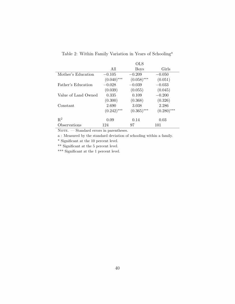
Table 2: Within Family Variation in Years of Schoolinga

OLSAll Boys Girls

Mother’s Education −0.105 −0.209 −0.050(0.040)∗∗∗ (0.058)∗∗∗ (0.051)

Father’s Education −0.028 −0.039 −0.033(0.039) (0.055) (0.045)

Value of Land Owned 0.335 0.109 −0.200(0.300) (0.368) (0.326)

Constant 2.690 3.038 2.286(0.242)∗∗∗ (0.365)∗∗∗ (0.280)∗∗∗

R2 0.09 0.14 0.03Observations 124 97 101Note. — Standard errors in parentheses.a : Measured by the standard deviation of schooling within a family.* Significant at the 10 percent level.** Significant at the 5 percent level.*** Significant at the 1 percent level.

40

Table 3: Mean Education by Birth Order

All Boys GirlsBirth Order Mean Obs Mean Obs. Mean Obs.

1 9.23 125 8.57 58 9.80 672 9.23 124 8.40 60 10.01 643 9.13 115 8.42 61 9.92 544 8.78 104 8.20 62 9.71 415 9.47 87 8.81 48 10.28 396 9.13 69 8.96 31 9.26 387 9.07 53 8.89 28 9.28 258 8.67 40 8.50 24 8.94 169 9.00 27 9.29 17 8.50 1210 8.66 22 8.00 10 9.58 1211 7.64 14 6.00 6 8.80 812 7.8 5 6.33 3 10.00 213 11.00 3 11.00 1 1.00 214 12.00 1 12.00 1 . 0

41

Table 4: Completed Education

Ordered Logit Estimation(1) (2) (3) (4)

Dummy for Girl 0.932∗∗∗ 1.356∗∗∗ 0.975∗∗∗ 0.927∗∗∗

(0.067) (0.152) (0.068) (0.113)Year of Birth −0.051∗∗∗ −0.028∗∗∗ 0.004∗∗ −0.039∗∗∗

(0.002) (0.002) (0.002) (0.002)Birth Order 0.245∗∗∗ 0.410∗∗∗

(0.009) (0.023)Birth Order × Mother’s Education −0.041∗∗∗

(0.005)Birth Order × Father’s Education −0.011∗∗∗

(0.002)Birth Order × Value of Land 0.401∗∗∗

(0.001)Birth Order × Dummy for Girl −0.089∗∗∗

(0.034)Relative Birth Order 0.860∗∗∗ 3.042∗∗∗

(0.137) (0.232)Relative Birth Order × Mother’s Education −0.182∗∗∗

(0.036)Relative Birth Order × Father’s Education −0.193∗∗∗

(0.016)Relative Birth Order × Value of Land 2.962∗∗∗

(0.461)Relative Birth Order × Dummy for Girl 0.159

(0.227)Observations 817 817 817 817Number of Households 125 125 125 125Note. — Standard errors in parentheses.* Significant at the 10 percent level.** Significant at the 5 percent level.*** Significant at the 1 percent level.

42

Table 5: Participation in Schoola

Conditional logit Estimation(1) (2) (3) (4)

Dummy for Girl 0.312 0.436 0.329 0.491(0.202) (0.424) (0.203) (0.436)

Age 0.771∗ 0.756∗ 0.796∗∗ 0.771∗

(0.394) (0.398) (0.395) (0.398)Age Squared −0.039∗∗∗ −0.039∗∗∗ −0.040∗∗∗ −0.040∗∗∗

(0.013) (0.013) (0.014) (0.013)Dummy for Age > 12 −1.638∗∗∗ −1.621∗∗∗ −1.635∗∗∗ −1.597∗∗∗

(0.522) (0.524) (0.523) (0.525)Year of Birth 0.074 0.081 0.156∗∗∗ 0.157∗∗∗

(0.083) (0.085) (0.050) (0.051)Birth Order 0.155 0.121

(0.198) (0.210)Birth Order × Mother’s Education −0.003

(0.002)Birth Order × Father’s Education 0.012

(0.011)Birth Order × Value of Land −0.075

(0.051)Birth Order × Dummy for Girl −0.021

(0.072)Relative Birth Order −0.365 −0.318

(0.701) (0.810)Relative Birth Order × Mother’s Education −0.024

(0.022)Relative Birth Order × Father’s Education 0.048

(0.038)Relative Birth Order × Value of Land −0.345

(0.365)Relative Birth Order × Dummy for Girl −0.276

(0.705)Observations 1122 1122 1122 1122Number of Households 226 226 226 226Note. — Standard errors in parentheses.a : Children aged 7 to 18 that spends a positive amount of time in school.* Significant at the 10 percent level.** Significant at the 5 percent level.*** Significant at the 1 percent level. 43

Table 6: Time Spent on School Activitiesa

Kyriazidou’s Method(1) (2) (3) (4)

Dummy for Girl 1.228∗ 7.915∗∗∗ 1.376∗∗ 3.909∗∗

(0.719) (1.467) (0.653) (1.928)Year of Birth 0.947∗∗∗ 0.560 2.461∗∗∗ 2.002∗∗∗

(0.346) (0.369) (0.281) (0.280)Age 4.805∗∗ 5.054∗∗∗ 6.435∗∗∗ 4.437∗∗

(1.939) (1.872) (1.751) (1.787)Age Squared −0.092 −0.106 −0.198∗∗ −0.104

(0.095) (0.091) (0.086) (0.087)Birth Order 2.096∗∗ 3.543∗∗∗

(0.886) (0.970)Birth Order × Mother’s Education 0.019

(0.021)Birth Order × Father’s Education 0.018

(0.026)Birth Order × Value of Land 0.204

(0.136)Birth Order × Dummy for Girl −1.116∗∗∗

(0.176)Relative Birth Order −8.712 −4.428

(2.452) (3.532)Relative Birth Order × Mother’s Education −0.172

(0.114)Relative Birth Order × Father’s Education 0.163∗∗

(0.065)Relative Birth Order × Value of Land 0.135

(2.881)Relative Birth Order × Dummy for Girl −4.653∗

(2.473)Observations 1470 1470 1470 1470Number of Households 201 201 201 201Note. — Standard errors in in parentheses.a : Number of hours spent in school by children aged 7 to 18.* Significant at the 10 percent level.** Significant at the 5 percent level.*** Significant at the 1 percent level.

44

Table 7: Simulation - Number of Children

Birth Order c = 0.25 c = 0.5 c = 0.75 c = 1.01 2000 2000 2000 20002 2000 2000 2000 12533 2000 2000 1510 7534 2000 2000 808 3955 2000 1961 334 1976 2000 1011 90 757 2000 89 10 158 1918 2 0 3

53otes: 2000 households with R = 100, k = 10 and α = 0.9.

45

Table 8: Simulation - Schooling and Human Capital

Schooling InputAverage Difference to Family Mean

Birth Order c = 0.25 c = 0.5 c = 0.75 c = 1.0 c = 0.25 c = 0.5 c = 0.75 c = 1.01 1.9 5.5 13.4 23.2 −0.0 −0.1 −1.7 −9.02 1.9 5.5 13.3 20.7 −0.0 −0.1 −1.7 3.63 1.9 5.6 12.8 20.5 0.0 −0.0 1.2 9.14 1.9 5.6 11.6 17.1 −0.0 −0.1 3.2 9.25 1.9 5.6 11.5 15.9 −0.0 −0.0 5.4 10.16 1.9 5.2 11.1 14.8 −0.0 0.7 6.7 10.57 1.9 4.5 6.8 9.3 −0.0 1.5 3.8 6.48 1.9 4.5 9.4 0.0 2.6 7.5

Human Capital OutcomeAverage Difference to Family Mean

Birth Order c = 0.25 c = 0.5 c = 0.75 c = 1.0 c = 0.25 c = 0.5 c = 0.75 c = 1.01 98.7 292.2 733.3 1229.7 −0.9 −11.1 −110.6 −495.62 98.6 293.7 729.2 1109.7 −0.9 −9.6 −114.7 198.13 100.1 300.2 699.7 1105.5 0.5 −3.1 86.2 510.44 98.6 293.8 623.2 897.5 −0.9 −9.5 209.0 501.05 98.9 294.7 619.4 837.0 −0.6 −1.0 334.8 551.86 98.9 270.6 610.8 803.0 −0.7 58.0 417.5 598.77 99.1 226.0 328.1 535.9 −0.5 110.1 219.1 408.18 99.3 198.2 387.4 4.1 134.0 319.2

Notes: 2000 households with R = 100, k = 10 and α = 0.9.

46

Table 9: Simulation - Summary Statistics

c = 0.25 c = 0.5 c = 0.75 c = 1.0Fertility 7.96 5.53 3.38 2.35

SchoolingMean Schooling Input (all) 1.90 5.67 15.06 32.18Mean Schooling Input (2+) 1.90 5.67 15.06 17.14First-born to family average −0.00 −0.13 −1.68 −14.29Last-born to family average −0.02 0.50 4.57 22.25Last-born - first-born 0.03 0.64 6.24 36.54

Human CapitalMean Human Capital (all) 99.55 303.34 843.92 1725.29Mean Human Capital (2+) 99.55 303.34 843.92 911.59First-born to family average −0.88 −11.10 −110.61 −791.03Last-born to family average 3.92 41.74 298.45 1228.11Last-born - first-born 4.80 52.83 409.06 2019.14Notes: 2000 households with R = 100, k = 10 and α = 0.9.

47

Table 10: Simulation - Resources and Costs of Children

R = 80 R = 100 R = 120k = 10 k = 20 k = 10 k = 20 k = 10 k = 20

Fertility 2.70 1.58 3.38 1.82 4.03 2.10Schooling

Mean Schooling Input (All) 17.17 26.20 15.06 30.12 14.79 32.19Mean Schooling Input (2+) 13.47 12.34 15.06 16.29 14.79 19.56First-born to family average −3.07 −6.08 −1.68 −7.04 −1.69 −7.37Last-born to family average 5.34 6.53 4.57 8.43 5.40 9.87Last-born - first-born 8.41 12.60 6.24 15.47 7.09 17.24

Human CapitalMean Human Capital (All) 975.20 1293.45 843.92 1534.55 830.94 1680.88Mean Human Capital (2+) 723.86 522.48 843.92 733.24 830.94 927.51First-born to family average −206.72 −345.46 −110.61 −416.11 −111.17 −445.51Last-born to family average 350.28 371.18 298.45 492.96 351.43 587.01Last-born - first-born 557.00 716.65 409.06 909.07 462.60 1032.52Notes: 2000 households with α = 0.9 and c = 0.75.

48

Table 11: Completed Education

Fixed Effects Estimation(1) (2) (3) (4)

Dummy for Girl 0.929∗∗∗ 1.239∗∗∗ 0.929∗∗∗ 1.064∗∗∗

(0.181) (0.334) (0.183) (0.316)Year of Birth −0.137∗∗∗ −0.123∗∗∗ −0.011 −0.062∗

(0.044) (0.045) (0.031) (0.033)Birth Order 0.429∗∗∗ 0.674∗∗∗

(0.111) (0.135)Birth Order × Mother’s Education −0.030∗

(0.017)Birth Order × Father’s Education −0.034∗∗

(0.014)Birth Order × Value of Land 0.331∗∗

(0.129)Birth Order × Dummy for Girl −0.074

(0.063)Relative Birth Order 0.765 4.162∗∗∗

(0.564) (1.009)Relative Birth Order × Mother’s Education −0.269∗∗

(0.112)Relative Birth Order × Father’s Education −0.250∗∗

(0.103)Relative Birth Order × Value of Land 1.511∗∗

(0.766)Relative Birth Order × Dummy for Girl −0.302

(0.544)Observations 790 790 790 790Number of Households 125 125 125 125Note. — Standard errors in parentheses.* Significant at the 10 percent level.** Significant at the 5 percent level.*** Significant at the 1 percent level.

49

Figure 1: The Distribution of Time Spent on School Activities

50