Boltzmann’s dilemma – an introduction to statistical

mechanics via the Kac ring

Georg A. Gottwald∗ Marcel Oliver†

February 23, 2009

Abstract

The process of coarse-graining—here, in particular, of passing from a determinis-

tic, simple, and time-reversible dynamics at the microscale to a typically irreversible

description in terms of averaged quantities at the macroscale—is of fundamental im-

portance in science and engineering. At the same time, it is often difficult to grasp

and, if not interpreted correctly, implies seemingly paradoxical results. The kinetic

theory of gases, historically the first and arguably most significant example, occupied

physicists for the better part of the 19th century and continues to pose mathematical

challenges to this day.

In these notes, we describe the so-called Kac ring model, suggested by Mark Kac

in 1956, which illustrates coarse-graining in a setting so simple that all aspects can be

exposed both through elementary, explicit computation and through easy numerical

simulation. In this setting, we explain a Boltzmannian “Stoßzahlansatz”, ensemble

averages, the difference between ensemble averaged and “typical” system behavior,

and the notion of entropy.

1 Introduction

The concept that matter is composed of atoms and molecules is nowadays a truism, muchlike saying that the earth is a sphere and that it orbits around the sun. However, reconcilingan atomistic description of nature with our everyday experience of how the world works isa so much harder question that any serious explanation is usually deferred to an advancedundergraduate or graduate course in statistical physics.

The point of difficulty is not that, at the atomic level, we should be using quantummechanics, that relativistic effects may not be ignored, or that we should really start out with

∗School of Mathematics and Statistics, University of Sydney, NSW 2006, Australia.

Email: gottwald@maths.usyd.edu.au†School of Engineering and Science, Jacobs University, 28759 Bremen, Germany.

Email: oliver@member.ams.org

1

a description of the subatomic structure which itself is described by highly elaborate quantumtheories. Rather, the issue is much more general and, from the point of view of constructingmathematical models for any kind of observable process, much more fundamental: all theoriesof microscopic physics are governed by laws that are invariant under reversal of time—theevolution of the system can be traced back into the past by the same evolution equationthat governs the prediction into the future. Processes on macroscopic scales, on the otherhand, are manifestly irreversible. Fluids mix, but cannot be unmixed by the same process(with some notable exceptions [15, 8]). Steam engines use differences in temperature to douseful mechanical work; in doing so, heat flows from hot to cold, eventually equilibratesand reduces the potential for doing further mechanical work. Particularly stark examples ofirreversibility are birth, aging, and dying.

Scientists are also completely comfortable with mathematical modeling at the macroscale. Classical thermodynamics, reaction-diffusion equations, empirical laws for frictionand drag, and many other equations of engineering and science provide extremely accuratequantitative descriptions of observable, irreversible phenomena without reference to the un-derlying micro-physics. This begs an obvious question. Since we have now two presumablyaccurate, quantitative mathematical models of the same system, how does one embed intothe other? And if such a relation can be established, how can it even be that one of thesedescriptions is reversible whereas the other is not?

The short answer, pioneered by Maxwell and Boltzmann in the context of a kinetictheory of gases, is that the macroscopic laws are a fundamentally statistical description—they represent the most probable behavior of the system. At the same time, most microscopicrealizations of a macroscopic state remain close to the most probable behavior for a long,but finite interval of time. The long answer, which provides quantitative definiteness andmathematical rigor, is, in most cases, truly long and difficult. Nonetheless, there are anumber of toy models, most notably the Ehrenfests’ urn model [5] and Mark Kac’s ring model[6], which provide a caricature of the underlying issues while being simple enough that theycan be exposed through elementary and explicit computation. Many of the mathematicalquestions underlying the kinetic theory of gases remain open, though, and are central tomaking advances in an increasing number of applications of kinetic theory to the modelingof complex systems, e.g. in biology, climate, semiconductors, and economics [2].

These notes are structured as follows. After a brief historical introduction, Section 3describes the Kac ring model and the Kac ring analog of the Stoßzahlansatz in kinetic theory.In Section 4, we define and compute ensemble averages. The conditions under which typicalexperiments will follow the averaged behavior are discussed, by computing the variance ofthe ensemble, in Section 5. Section 6 presents the continuum limit of the Kac ring andSection 7 the concept of entropy. The paper closes with a short mentioning of the Ehrenfestmodel, an extended general summary and discussion, and a section in which we commenton some of our experiences when teaching these lectures.

Our presentation follows, in parts, the book chapters by Dorfman [3] and Schulman [12].We have not seen a detailed quantitative discussion of the variance and of the continuumlimit elsewhere, though they were certainly known to Kac. The notes also contain a good

2

number of exercises, from easy or review-type topics to more advanced open-ended questionswhich reach beyond a first acquaintance with the subject.

2 Historical background

The questions we address here have historically been asked in face of the apparent conflictbetween classical thermodynamics and mechanics which followed on the footsteps of thechemists’ realization that gases are composed of discrete, apparently indivisible molecules.We shall give a brief account of this background, not to strive for completeness and accuracy(this would require a more major endeavor than anything we attempt here), but to convey asense that the concepts ultimately provided by Maxwell and Boltzmann constituted a majorbreakthrough in scientific thought. For more historic detail, see [10, 13, 17] and referencestherein.

Up until the end of the 18th century, the mathematical theories of thermodynamics andmechanics were studied largely in parallel. When Isaac Newton (1643–1727) wrote down thefoundations of classical mechanics and Robert Boyle (1627–1691) announced his law whichrelates the volume of a gas to the pressure, there was little concrete evidence that the twowere related at all. Still, the idea that heat is a consequence of the motion of atomic particlesdates back to at least this era and is discussed in the works of Boyle, Newton, and later ofDaniel Bernoulli (1700–1782) who, in 1738, first formulated a quantitative kinetic theory.This work, however, was largely forgotten for another century.

The issue got new urgency when John Dalton (1766–1844) and others laid the foundationsfor the modern atomic theory of matter and Amedeo Avogadro (1776–1856) postulatedthat the number of molecules per volume is only a function of temperature and pressure,independent of the chemical composition of a gas. A number of scientists, most notableHerapath, Waterson, Joule, and Clausius (who is also credited with stating the second lawof thermodynamics in terms of entropy), worked on kinetic descriptions of gases.

The real break-through in the development of kinetic theory, however, is due to JamesClerk Maxwell (1831–1879) and Ludwig Boltzmann (1844–1906). Maxwell was the first tolook at gases from a probabilistic point of view and computed the equilibrium probabilitydistribution of molecular velocities (which, in fact, is a manifestation of the central limittheorem). In a seminal 1867 paper, Maxwell introduces an evolution equation for (momentsof) the probability density of finding a molecule of given velocity at a given location inspace, which he uses to derive equations for the macroscopic dynamics of gases. The crucialunderlying assumption, which Boltzmann later called the Stoßzahlansatz (which literallytranslates as “collision number hypothesis” and is often referred to as the molecular chaos

assumption), is the statistical independence of the probability densities of colliding molecules(i.e. the model has no memory of trajectories of individual molecules).

Among Boltzmann’s most prominent contributions is an 1872 paper in which he writesout a reformulation of Maxwell’s kinetic equation, which is nowadays referred to as theBoltzmann equation, from which he deduces that there is a quantity H which is nonincreasingalong solution trajectories of the Boltzmann equation and, in particular, remains constant

3

for Maxwell’s equilibrium distribution. Boltzmann equated the negative of his H-functionwith Clausius’ thermodynamic entropy and thus claimed to have proved the second law ofthermodynamics via statistical mechanics.

Boltzmann’s work faced severe criticism, essentially on two levels. His contemporariesasked, almost immediately after publication, how a microscopically time-reversible and re-current system can give rise to a macroscopic description which is neither. The two famousobjections became known as Loschmidt’s paradox and Zermelo’s paradox. Josef Loschmidt(1821–1895) and others pointed out that system trajectories in classical mechanics, the start-ing point of Boltzmann’s derivation, are deterministic and time-reversible—see Exercise 1below. Therefore, the reasoning goes, Boltzmann’s result, namely, the manifestly irreversibleH-theorem, cannot possibly be correct. (In fact, Maxwell himself had already addressed andessentially resolved the reversibility paradox several years earlier.) Ernst Zermelo (1871–1953) gave a new, general proof of Poincare’s recurrence theorem which showed that thetheorem is indeed applicable to the situation considered by Boltzmann [18]. Poincare’s the-orem states that a dynamical system with constant energy in a compact phase space musteventually return to its initial state within arbitrary precision for almost all initial data [9].Thus, surely, H cannot always decrease but must also increase as the system recurs to itsinitial configuration. While Zermelo’s proof is based on abstract measure theory, the issuecan be easily understood in a finite setting. It hinges on the property of reversibility—seeExercise 2.

Exercise 1. Newton’s second law of mechanics for a particle of mass m situated at positionx(t) moving with velocity v(t) and subject to a force F (x(t)) can be written

dx

dt= v , (1a)

mdv

dt= F (x(t)) . (1b)

Show that the particle satisfies the same equation with t replaced by the reversed time s = −tand v replaced by u = −v.

Exercise 2. Show that in a time-discrete, reversible, system with a finite number of statesany orbit must return to its initial state after a finite number of steps.

Remark 1. Reversibility applies not only to classical mechanics, but, in a more generalsense, to all physical laws governing the fundamental forces of nature. The resulting appar-ent discrepancy with our macroscopic experience of the world is often considered a majorphilosophical issue. We take the view that the apprehension of coarse-graining as a modelingparadigm is, largely, a mathematical question. Once the operational issues are understood,the urgency of philosophical debate is greatly diminished.

The second strand of objections to Boltzmann’s approach concerns the justification ofthe Stoßzahlansatz and of the subsequent reduction of the macroscopic dynamics to an evo-lution equation for a one-particle probability distribution function. While it is now generally

4

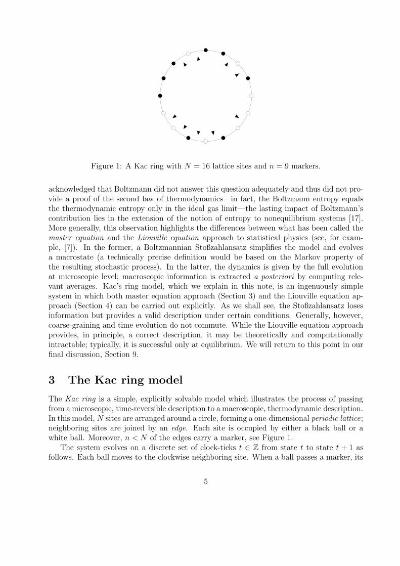
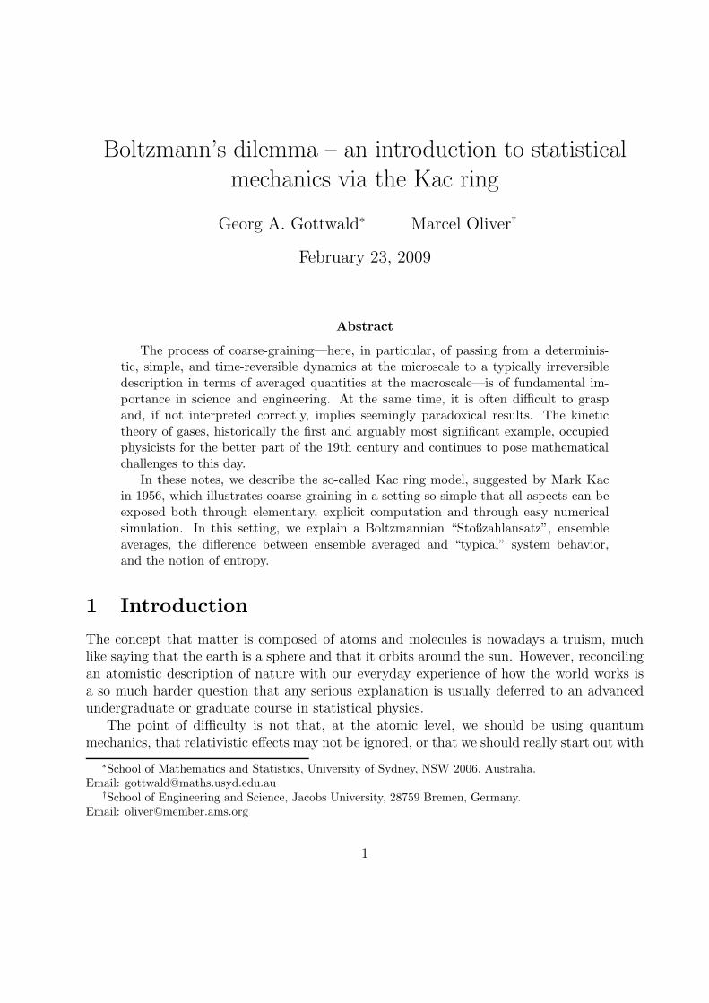
Figure 1: A Kac ring with N = 16 lattice sites and n = 9 markers.

acknowledged that Boltzmann did not answer this question adequately and thus did not pro-vide a proof of the second law of thermodynamics—in fact, the Boltzmann entropy equalsthe thermodynamic entropy only in the ideal gas limit—the lasting impact of Boltzmann’scontribution lies in the extension of the notion of entropy to nonequilibrium systems [17].More generally, this observation highlights the differences between what has been called themaster equation and the Liouville equation approach to statistical physics (see, for exam-ple, [7]). In the former, a Boltzmannian Stoßzahlansatz simplifies the model and evolvesa macrostate (a technically precise definition would be based on the Markov property ofthe resulting stochastic process). In the latter, the dynamics is given by the full evolutionat microscopic level; macroscopic information is extracted a posteriori by computing rele-vant averages. Kac’s ring model, which we explain in this note, is an ingenuously simplesystem in which both master equation approach (Section 3) and the Liouville equation ap-proach (Section 4) can be carried out explicitly. As we shall see, the Stoßzahlansatz losesinformation but provides a valid description under certain conditions. Generally, however,coarse-graining and time evolution do not commute. While the Liouville equation approachprovides, in principle, a correct description, it may be theoretically and computationallyintractable; typically, it is successful only at equilibrium. We will return to this point in ourfinal discussion, Section 9.

3 The Kac ring model

The Kac ring is a simple, explicitly solvable model which illustrates the process of passingfrom a microscopic, time-reversible description to a macroscopic, thermodynamic description.In this model, N sites are arranged around a circle, forming a one-dimensional periodic lattice;neighboring sites are joined by an edge. Each site is occupied by either a black ball or awhite ball. Moreover, n < N of the edges carry a marker, see Figure 1.

The system evolves on a discrete set of clock-ticks t ∈ Z from state t to state t + 1 asfollows. Each ball moves to the clockwise neighboring site. When a ball passes a marker, its

5

color changes.The dynamics of the Kac ring is time-reversible and has recurrence. When the direction

of movement along the ring is reversed, the balls retrace their past color sequence withoutchange to the “laws of physics”. Moreover, after N clock ticks, each ball has reached itsinitial site and changed color n times. Thus, if n is even, the initial state recurs; if n is odd,it takes at most 2N clock ticks for the initial state to recur.

Let B(t) denote the total number of black balls and b(t) the number of black balls just infront of a marker; let W (t) denote the number of white balls and w(t) the number of whiteballs in front of a marker. Then

B(t + 1) = B(t) + w(t) − b(t) (2)

and, similarly,

W (t + 1) = W (t) + b(t) − w(t) . (3)

We will study the behavior of ∆(t) = B(t) − W (t). Clearly,

∆(t + 1) = B(t + 1) − W (t + 1) = ∆(t) + 2 w(t) − 2 b(t) . (4)

Note that W , B, and ∆ are macroscopic quantities, describing a global feature of the systemstate; w and b, on the other hand, contain local information about individual sites—theycannot be computed without knowing the location of each marker and the color of the ballat every site. A key feature of this system is that the evolution of the global quantities isnot computable only from macroscopic state information. In other words, it is not possibleto eliminate b and w from equations (2)–(4). This is known as the closure problem.

When the markers are distributed at random, the probability that a particular site isoccupied by a marker is given by

µ ≡ n

N=

b

B=

w

W. (5)

For an actual realization of the Kac ring these relations will generally not be satisfied.However, by assuming that they hold anyway, we can overcome the closure problem. Thisassumption is the analogue of Maxwell and Boltzmann’s Stoßzahlansatz. It effectively disre-gards the history of the system evolution; there is no memory of where the balls originatedand which markers they passed up to time t. However, we hope that this assumption repre-sents, in some sense, the typical behavior of large sized rings.

Under this “Stoßzahlansatz”, equation (4) becomes

∆(t + 1) = ∆(t) + 2 µ W (t) − 2 µ B(t) = (1 − 2 µ) ∆(t) . (6)

This recurrence immediately yields

∆(t) = (1 − 2 µ)t ∆(0) . (7)

6

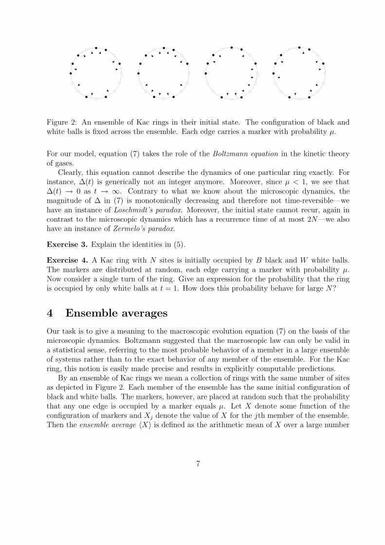
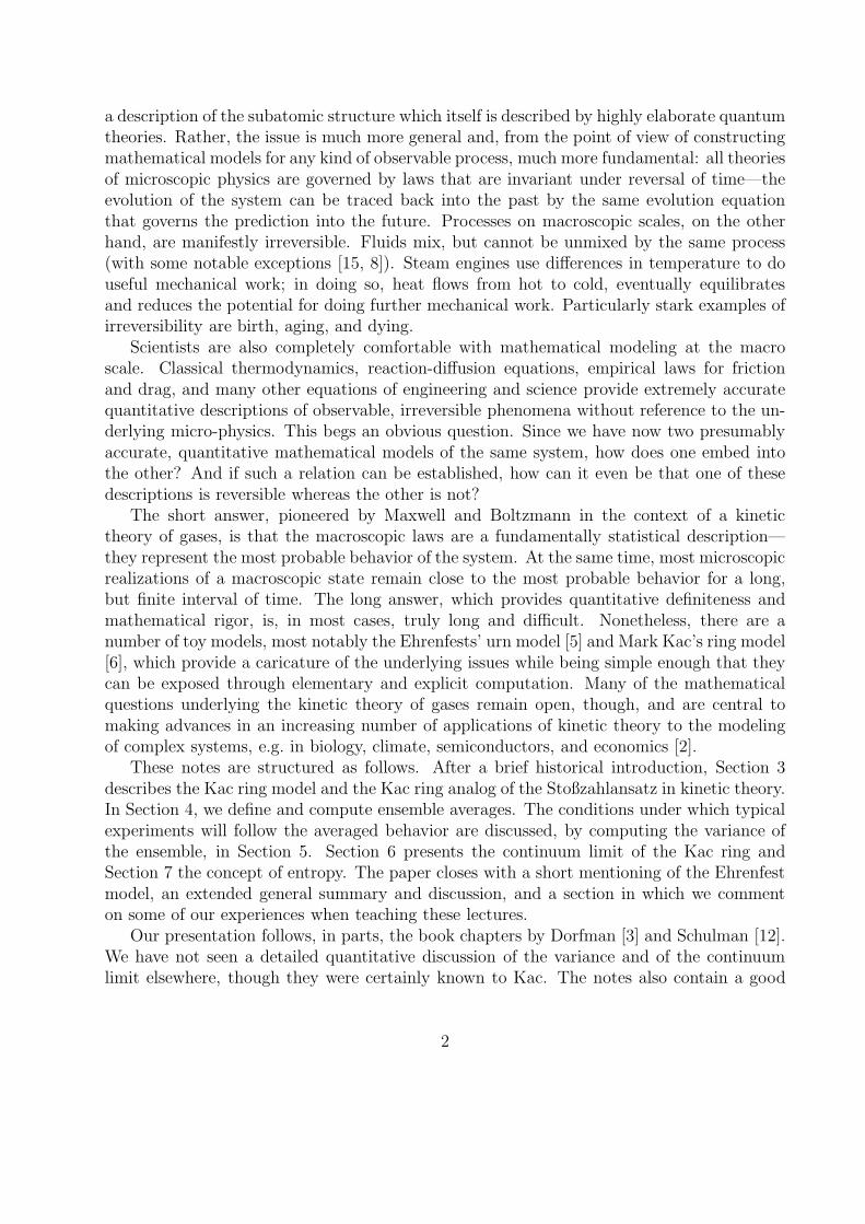
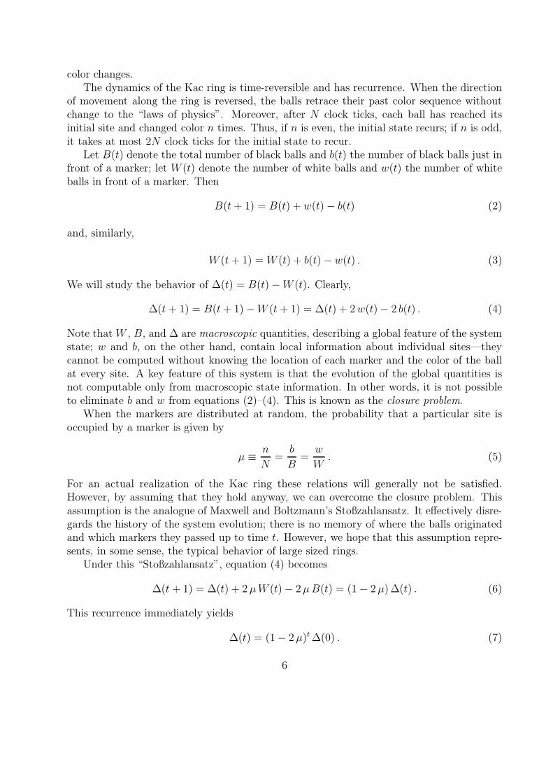
Figure 2: An ensemble of Kac rings in their initial state. The configuration of black andwhite balls is fixed across the ensemble. Each edge carries a marker with probability µ.

For our model, equation (7) takes the role of the Boltzmann equation in the kinetic theoryof gases.

Clearly, this equation cannot describe the dynamics of one particular ring exactly. Forinstance, ∆(t) is generically not an integer anymore. Moreover, since µ < 1, we see that∆(t) → 0 as t → ∞. Contrary to what we know about the microscopic dynamics, themagnitude of ∆ in (7) is monotonically decreasing and therefore not time-reversible—wehave an instance of Loschmidt’s paradox. Moreover, the initial state cannot recur, again incontrast to the microscopic dynamics which has a recurrence time of at most 2N—we alsohave an instance of Zermelo’s paradox.

Exercise 3. Explain the identities in (5).

Exercise 4. A Kac ring with N sites is initially occupied by B black and W white balls.The markers are distributed at random, each edge carrying a marker with probability µ.Now consider a single turn of the ring. Give an expression for the probability that the ringis occupied by only white balls at t = 1. How does this probability behave for large N?

4 Ensemble averages

Our task is to give a meaning to the macroscopic evolution equation (7) on the basis of themicroscopic dynamics. Boltzmann suggested that the macroscopic law can only be valid ina statistical sense, referring to the most probable behavior of a member in a large ensembleof systems rather than to the exact behavior of any member of the ensemble. For the Kacring, this notion is easily made precise and results in explicitly computable predictions.

By an ensemble of Kac rings we mean a collection of rings with the same number of sitesas depicted in Figure 2. Each member of the ensemble has the same initial configuration ofblack and white balls. The markers, however, are placed at random such that the probabilitythat any one edge is occupied by a marker equals µ. Let X denote some function of theconfiguration of markers and Xj denote the value of X for the jth member of the ensemble.Then the ensemble average 〈X〉 is defined as the arithmetic mean of X over a large number

7

of realizations, i.e.,

〈X〉 = limM→∞

1

M

M∑

j=1

Xj . (8)

In the language of (finite) probability, each particular configuration of markers is referredto as outcome from among the sample space S of all possible configurations of markers. Theprocess of choosing a random configuration of markers is called a trial. It is always assumedthat trials are independent, i.e. that the result of one trial does not depend on any past trials.We now recognize X as a function X : S → R; any such function is referred to as a random

variable. Thus, ensemble average is nothing but the expected value of a random variable, andcan be computed as follows. As the system is finite, X will take one of x1, . . . , xI possiblevalues (“macrostates”) with corresponding probabilities p1, . . . , pI . Then

〈X〉 =

I∑

i=1

pi xi . (9)

The identification of (8) and (9) is due to the definition of probability pi of the event X = xias its relative frequency of occurrence in a large number of trials. (In general, the term event

refers to a subset of the sample space.)

Exercise 5. Verify the identity of (8) and (9) explicitly for the following simple case. Con-sider an ensemble of systems which can be in one of two states. State 1 occurs with proba-bility p1 where X takes the value x1 = 1; state 2 occurs with probability p2 = 1 − p1 whereX takes the value x2 = 0.

Returning to the Kac ring, we formalize the microscopic laws of evolution as follows.Let χi(t) denote the color of the ball occupying the ith lattice site at time t, with value1 representing black and value −1 representing white. Further, let mi = −1 denote thepresence, and mi = 1 denote the absence of a marker on the edge connecting sites i andi + 1. Then the recurrence relation for stepping from t to t + 1 reads

χi+1(t + 1) = mi χi(t) . (10)

This expression makes sense for any i, t ∈ Z if we identify χ0 ≡ χN , χ1 ≡ χN+1, and soon—the lattice is periodic with period N . Similarly, we have m0 ≡ mN , m1 ≡ mN+1, and soon. Then

∆(t) =N

∑

i=1

χi(t) =N

∑

i=1

mi−1 χi−1(t − 1) = . . . =N

∑

i=1

mi−1 mi−2 · · ·mi−t χi−t(0) . (11)

Exercise 6. Verify, using (11), that ∆(2N) = ∆(0).

Equipped with the above definition and recipe for computing the ensemble average, wewish to compute the evolution of 〈∆(t)〉. Since averaging involves taking sums and therefore

8

distributes over sums, and since only the marker positions, but not the initial configurationof balls, may differ across the ensemble, we can pull the sum and the χi(0) out of the averageand obtain

〈∆(t)〉 =

N∑

i=1

〈mi−1 mi−2 · · ·mi−t〉χi−t(0) . (12)

Since all lattice edges have equal probability of carrying a marker, the average in (12) mustbe invariant under index shifts. In particular, 〈mi−1 mi−2 · · ·mi−t〉 = 〈m1 m2 · · ·mt〉, so that

〈∆(t)〉 = 〈m1 m2 · · ·mt〉N

∑

i=1

χi−t(0) = 〈m1 m2 · · ·mt〉∆(0) . (13)

Our remaining task is to find an explicit expression for 〈m1 m2 · · ·mt〉, a quantity which onlydepends on the distribution of the markers, but not on the balls. We distinguish two cases.

When 0 ≤ t < N , there are no periodicities—all factors m1, . . . , mt are independent.The value of the product is 1 for an even number of markers, and −1 for an odd number ofmarkers. Thus, (9) takes the form

〈m1 m2 · · ·mt〉 =t

∑

j=0

(−1)j pj(t) , (14)

where pj(t) denotes the probability of finding j markers on t consecutive edges. The markersfollow a binomial distribution, so that

pj(t) = µj (1 − µ)t−j

(

t

j

)

, (15)

and, using the binomial theorem,

〈m1 m2 · · ·mt〉 =

t∑

j=0

(

t

j

)

(−µ)j (1 − µ)t−j = (1 − 2 µ)t . (16)

Inserting this expression into (13), we obtain

〈∆(t)〉 = (1 − 2 µ)t ∆(0) , (17)

the same expression (7) we obtained through our initial “molecular chaos assumption”.This result is encouraging, because it shows that the relatively crude “Stoßzahlansatz”

of Section 3 may be related to the average over a statistical ensemble. In general, however,one cannot expect exact identity. Indeed, even for the Kac ring, the following computationshows that when t > N , the two concepts diverge.

Exercise 7. Derive (15). Proceed in two steps. First, what is the probability of finding amarker on each of the the first j edges, and no marker on the next t − j edges? Second,correct for the resulting undercount by considering all possible distinct permutations of theseedges.

9

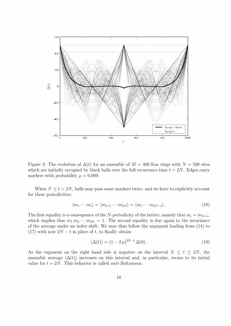
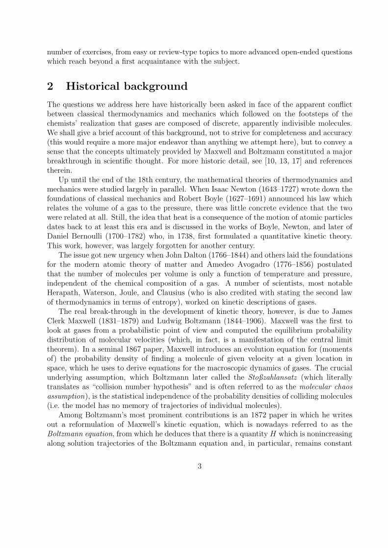
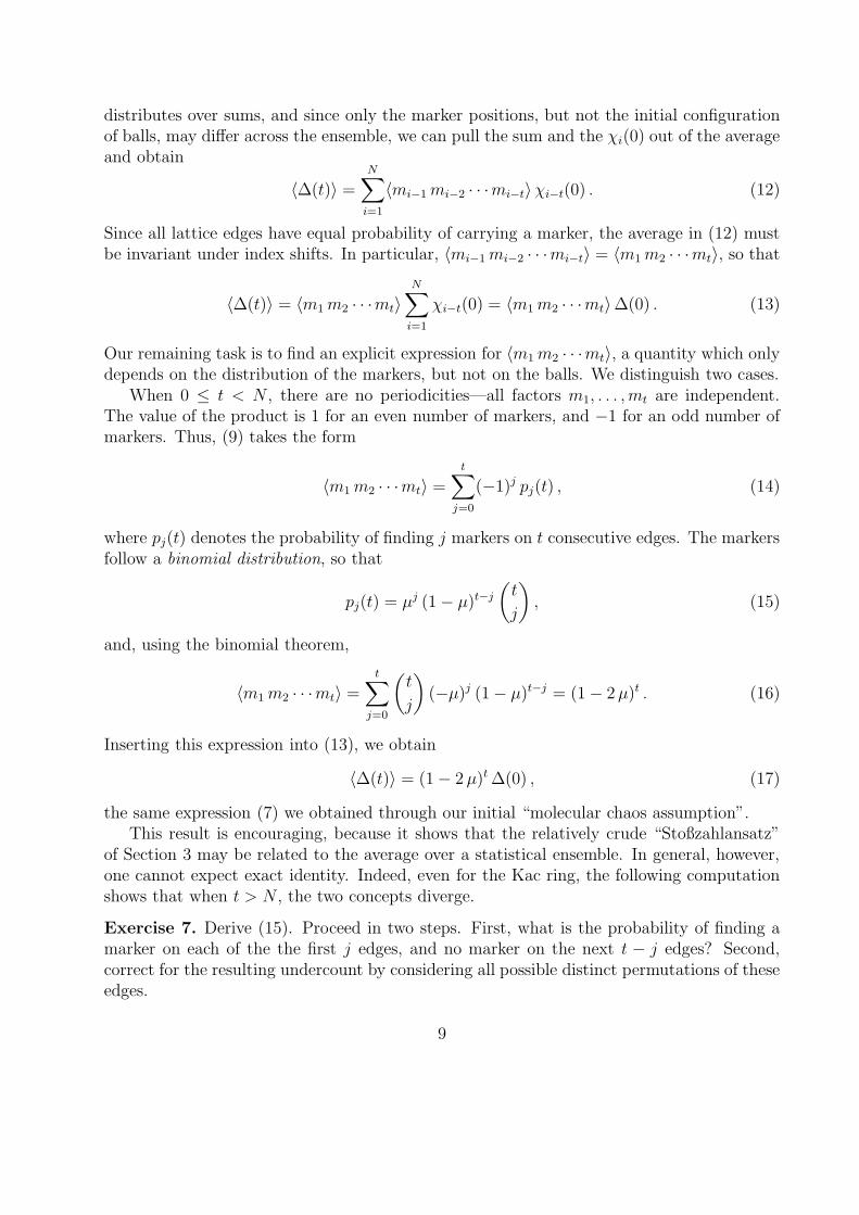
Figure 3: The evolution of ∆(t) for an ensemble of M = 400 Kac rings with N = 500 siteswhich are initially occupied by black balls over the full recurrence time t = 2N . Edges carrymarkers with probability µ = 0.009.

When N ≤ t < 2N , balls may pass some markers twice, and we have to explicitly accountfor these periodicities:

〈m1 · · ·mt〉 = 〈mt+1 · · ·m2N 〉 = 〈m1 · · ·m2N−t〉 . (18)

The first equality is a consequence of the N -periodicity of the lattice, namely that mi = mN+i,which implies that m1 m2 · · ·m2N = 1. The second equality is due again to the invarianceof the average under an index shift. We may thus follow the argument leading from (14) to(17) with now 2N − t in place of t, to finally obtain

〈∆(t)〉 = (1 − 2 µ)2N−t ∆(0) . (19)

As the exponent on the right hand side is negative on the interval N ≤ t ≤ 2N , theensemble average 〈∆(t)〉 increases on this interval and, in particular, recurs to its initialvalue for t = 2N . This behavior is called anti-Boltzmann.

10

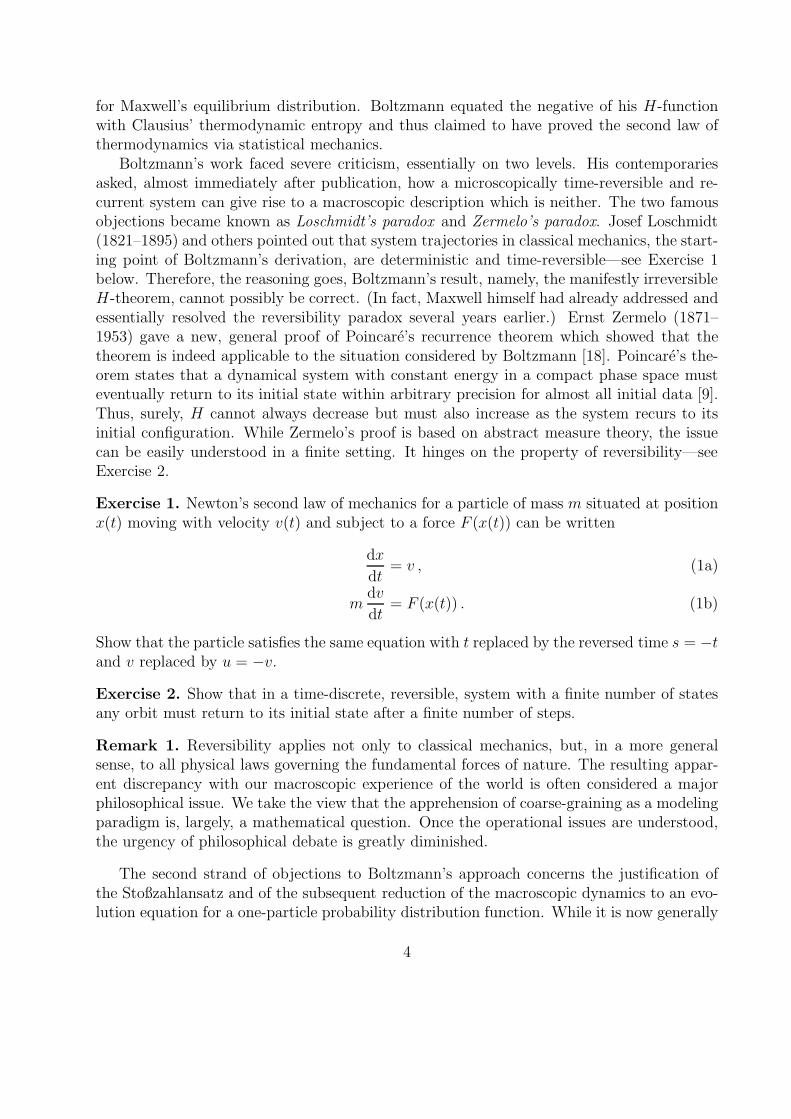
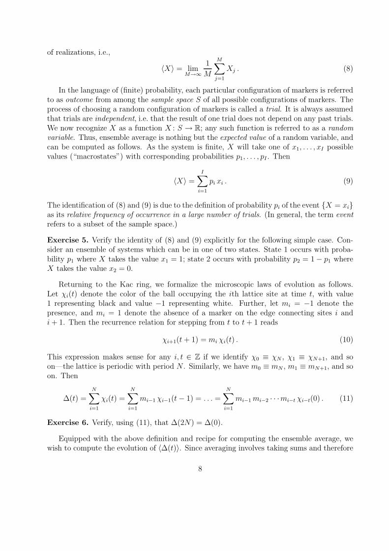
Figure 4: Ensemble of larger sized Kac rings with N = 2000, all other parameters are as inFigure 3.

Figure 3 shows a simulation of an ensemble of Kac rings. Clearly visible is the recurrenceat t = 2N . The sample mean compares well with the predicted ensemble average, equations(17) and (19). The theoretical predictions are not explicitly drawn, but they would notvisibly depart from the sample mean except near the half-recurrence time t = N when eachindividual trajectory either recurs or arrives at the negative of its initial value. The half-recurrence time is also the time of maximal variance, as we will discuss in the followingSection 5, so that the size of our sample is simply too small to get a good experimentalprediction of the mean. Figure 3 also shows that some realizations have large departuresfrom the mean while most stay close at least for times t ≪ N . We shall make this observationmore precise in Section 6. Finally, note that the expected number of markers per ring inFigure 3 is 4.5. Thus, with high probability, the ensemble contains rings with zero, one, andtwo markers. Trajectories corresponding to each of these cases are clearly visible. (Can youidentify them?)

Figure 4 shows the behavior of an ensemble of larger size Kac rings with all other param-eters kept fixed. For larger rings the probability of having a ring without a marker or with

11

just a few markers becomes negligible. Thus, the sample shown does not contain trajectoriescorresponding to almost marker-free members of the ensemble.

5 Is average behavior typical?

In the previous section, we have shown that the Stoßzahlansatz leads to a macroscopicequation that represents the averaged behavior of an ensemble of Kac rings for times t ≤ N .This, however, does not imply that the ensemble average represents in some way “typical”members of the ensemble, or that it is even close to any individual system trajectory. Forexample, at the half-recurrence time t = N , each ball is back at its initial position witha possible global change of color whenever the total number of markers is odd, so that∆(N) = ±∆(0) while, by (17), 〈∆(N)〉 is close to zero. For small t, on the other hand, mostmembers of the ensemble stay close to the sample mean. Both these regimes are clearlyvisible in Figures 3 and 4. How can we quantify this observed behavior?

We will answer this question by estimating the variance of the ensemble as a function oft, which is a measure of how much the individual members of the ensemble disperse aboutthe mean. More precisely,

Var[∆(t)] =⟨(

∆(t) − 〈∆(t)〉)2⟩

. (20)

In particular, the variance is zero if all members coincide with the mean and Var[∆] = d2 ifall members are situated at distance ±d away from the mean. An easy computation givesan alternative expression, more amenable to computation,

Var[∆(t)] = 〈∆2(t)〉 − 〈∆(t)〉2 . (21)

The estimation of the variance follows essentially the same pattern as the computation ofthe ensemble mean in Section 4. By analogy with (11),

∆2(t) =

N∑

i,j=1

χi(t) χj(t)

=N

∑

i,j=1

mi−1 · · ·mi−t mj−1 · · ·mj−t χi−t(0) χj−t(0)

=

N/2−1∑

k=−N/2

N∑

i=1

mi−1 · · ·mi−t mi−1+k · · ·mi−t+k χi−t(0) χi−t+k(0) , (22)

where we have re-indexed one of the sums writing j = i + k, noting again the periodicity ofthe lattice. Moreover, for simplicity, we assume that N is even so that N/2 is an integer.Then taking averages and noting, once more, that the average over products of the mi isinvariant under index shifts, we find that

〈∆2(t)〉 =

N/2−1∑

k=−N/2

〈mt · · ·m1 mt+k · · ·m1+k〉N

∑

i=1

χi−t(0) χi−t+k(0) . (23)

12

To proceed, we have to answer the following question. How many independent terms arethere within the averaging brackets? If t < N/2, which we shall assume throughout, therecan certainly be no more than 2t independent factors. For small values of |k| < t, however,there are only |k| terms in the first group of factors which do not recur in the second groupof factors, and vice versa, for a total of 2|k| independent factors. We conclude, repeating theargument that previously led us from (14) to (17), that

〈mt · · ·m1 mt+k · · ·m1+k〉 = (1 − 2 µ)2min|k|,t . (24)

Hence,

〈∆2(t)〉 =

N/2−1∑

k=−N/2

(1 − 2 µ)2min|k|,tN

∑

i=1

χi−t(0) χi−t+k(0)

= (1 − 2 µ)2t

N/2−1∑

k=−N/2

N∑

i=1

χi−t(0) χi−t+k(0)

+t−1∑

k=1−t

(

(1 − 2 µ)2|k| − (1 − 2 µ)2t

) N∑

i=1

χi−t(0) χi−t+k(0)

= (1 − 2 µ)2t ∆2(0) +

t−1∑

k=1−t

(

(1 − 2 µ)2|k| − (1 − 2 µ)2t

) N∑

i=1

χi−t(0) χi−t+k(0) . (25)

The first term on the right, due to (17), equals ∆2(t), so that, using the definition of thevariance and the fact that the final sum of (25) has N terms of unit modulus,

Var[∆(t)] ≤ N

t−1∑

k=1−t

(

(1 − 2 µ)2|k| − (1 − 2 µ)2t

)

= N

(

21 − (1 − 2 µ)2t

1 − (1 − 2 µ)2− 1 − (2t − 1) (1 − 2 µ)2t

)

= N

(

1 − (1 − 2 µ)2t

2 µ (1 − µ)− 1 − (2t − 1) (1 − 2 µ)2t

)

(26)

Exercise 8. Show that the bound (26) for Var[∆(t)] is strictly increasing on 0 ≤ t ≤ N/2provided that 0 < µ < 1

2.

Exercise 9. Show that Var[∆(N)] = (1− (1−2µ)2N ) ∆2(0). Describe the behavior for largeN .

Exercise 10. Repeat the analysis of this section on the interval N/2 ≤ t ≤ N . You shouldfind that

Var[∆(t)] ≤ N

(

1 − (1 − 2 µ)2(N−t)

2 µ (1− µ)−1+(2t−N +1) (1−2 µ)2(N−t)−N (1−2 µ)2t

)

. (27)

13

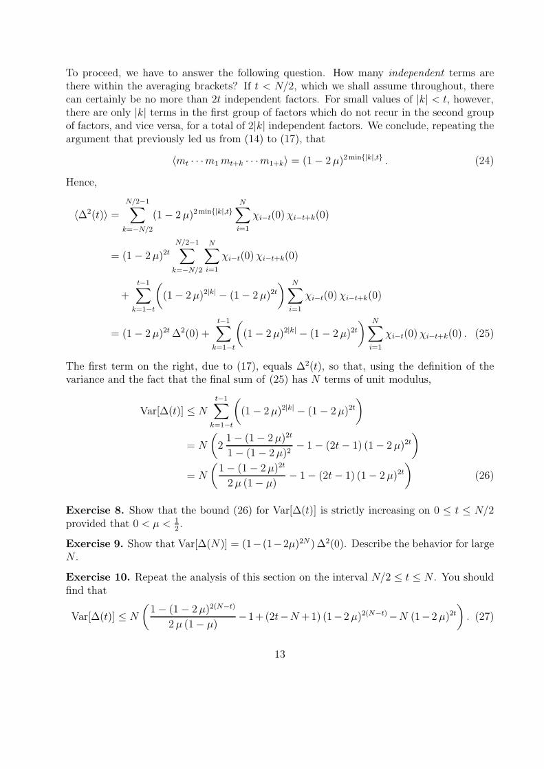
Figure 5: Magnified view of the time window 0 ≤ t ≤ N where the solution depicted inFigure 3 has “Boltzmann behavior”. Also depicted is the neighborhood with the radius ofone standard deviation (the square root of the variance) about the predicted ensemble meanas given by (26) and Exercise 10.

Remark 2. The bounds on the variance given by (26) and (27) hold with equality when|∆| = N initially. For this reason, the simulations in Figures 3–5 were so initialized.

The most important consequence we can draw from equations (26) and (27) is that thevariance scales like N , the standard deviation thus like

√N so long as we remain some

distance away from the half-recurrence time t = N . This behavior indicates that as N getslarge, the tube about 〈∆(t)〉 with a width of one standard deviation as depicted in Figure 5becomes narrow relative to ∆max = N . Thus, for short times and large N we can concludethat average behavior is typical. In the following section we shall make this asymptoticregime more precise.

14

6 Continuum limit

So far, everything we have talked about was fully discrete: a finite, integer number of sitesand markers and integer time t. The relative distances between neighboring discrete valuesfor W , B, and ∆, however, decrease as the size of the Kac ring increases. In addition, weshould, by now, have gotten a sense that large rings are “more typical” than smaller rings.

In the following, we will show how to pass to the “large ring limit” in a rigorous and pre-cisely defined sense. To begin, we note that simply letting N → ∞ in the above computationwill not work—everything will simply diverge in an uncontrolled manner. Therefore, the keyis to identify quantities which neither diverge nor go to zero and can thus carry nontrivialinformation about the system behavior into the limit.

The first of such quantities is almost obvious. What carries meaning is not the absolutedifference between the numbers of black and white balls ∆, but its magnitude relative to thetotal system size. We thus define

δ =∆

N, (28)

a measure for the grayness of the ring when looked at from a great distance. The graynessranges from δ = −1 corresponding to complete whiteness to δ = 1 corresponding to completeblackness, independent of the system size N . Though for a ring of a fixed size, δ takes onlya discrete set of values, every real δ ∈ [−1, 1] can be approximated arbitrarily closely by astate of a finite Kac ring of sufficiently large size. In terms of δ, equations (17) and (26) read

〈δ(t)〉 = (1 − 2 µ)t δ(0) (29)

and

Var[δ(t)] ≤ 1

N

(

1

2 µ (1− µ)− 1

)

, (30)

respectively.Second, we want the system within one unit of macroscopic time to be affected by very

many steps of the underlying microscopic Kac ring dynamics, in much the same way thatthe macroscopic grayness is affected by very many sites. This is achieved by introducing amacroscopic time variable τ which relates to microscopic time t via a scaling law of the form

τ =t

Nα(31)

for some exponent α > 0.Third, the behavior of the system within one unit of macroscopic time should be nontrivial

as N → ∞. Substituting (31) into (29), we see that it is necessary to have µ → 0 in thislimit. To be definite, we set

µ =1

2Nβ(32)

15

for some exponent β > 0. The prefactor 1/2 is for convenience, as we shall see below, anddoes not affect the nature of the result. We shall also require that β < 1, for else there wouldbe, on average, less than one marker per ring so that, in the limit, most realizations wouldbe uninteresting. With β ∈ (0, 1), the scaling law (32) expresses that the average number ofmarkers goes to infinity, but at a lesser rate than the size of the ring.

Plugging the scaling assumptions into (29), we find that

(1 − 2 µ)t =

(

1 − 1

Nβ

)τNα

→

0 if β < α

e−τ if β = α

1 if β > α ,

(33)

as N → ∞ for any fixed τ > 0. Hence, the condition α = β is necessary for obtaining anontrivial large system limit. Under this assumption, the limit Kac ring dynamics becomes

〈δ(τ)〉 = e−τ δ(0) . (34)

Moreover,

Var[δ] ≤ 1

N

1

2 µ (1 − µ)∼ 1

N

1

2 µ= Nβ−1 (35)

so that Var[δ] → 0 as N → ∞ (recall that β < 1). (Two sequences ak and bk are saidto be asymptotic, symbolically written ak ∼ bk, if limk→∞ ak/bk = 1.) This proves that,in the limit, almost all Kac rings follow the ensemble averaged dynamics; the macroscopicequation (34) describes the macroscopically observable behavior of almost any realization.Figure 6 illustrates the relation between scaled and unscaled variables, and the resultinglimiting behavior of the ensemble.

We finally remark that the scaling laws for t and µ may look arbitrary. This is correctin the sense that such scalings are generally outside the scope of the fundamental laws ofphysics and lack uniqueness in any strict mathematical sense. It is rather up to the ingenuityof the modeler to come up with a scaling which induces a mathematically tractable andwell-behaved limit—as in our example above—and, when modeling real-world systems, isconsistent with the relevant physical parameters.

7 Entropy

The term entropy was coined by Robert Clausius (1822-1888) in the 1860s, at the timeas a purely macroscopic concept without anticipation of an underlying probabilistic origin.It arises in the mathematical description of thermodynamical processes—closed systemsundergoing adiabatic transformations, to be precise—as a quantity which can only increasein time.

In popular accounts of statistical thermodynamics, entropy is often described as a mea-sure of “disorder”. This notion, however, is ill-defined and potentially misleading. Let us

16

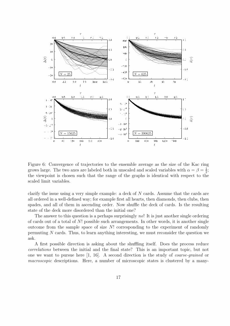
Figure 6: Convergence of trajectories to the ensemble average as the size of the Kac ringgrows large. The two axes are labeled both in unscaled and scaled variables with α = β = 1

2;

the viewpoint is chosen such that the range of the graphs is identical with respect to thescaled limit variables.

clarify the issue using a very simple example: a deck of N cards. Assume that the cards areall ordered in a well-defined way; for example first all hearts, then diamonds, then clubs, thenspades, and all of them in ascending order. Now shuffle the deck of cards. Is the resultingstate of the deck more disordered than the initial one?

The answer to this question is a perhaps surprisingly no! It is just another single orderingof cards out of a total of N ! possible such arrangements. In other words, it is another singleoutcome from the sample space of size N ! corresponding to the experiment of randomlypermuting N cards. Thus, to learn anything interesting, we must reconsider the question weask.

A first possible direction is asking about the shuffling itself. Does the process reducecorrelations between the initial and the final state? This is an important topic, but notone we want to pursue here [1, 16]. A second direction is the study of coarse-grained ormacroscopic descriptions. Here, a number of microscopic states is clustered by a many-

17

to-one map into a much smaller number of macroscopic states. We can then talk aboutmacroscopic states with relatively many microscopic realizations members as being moredisordered than those with relatively fewer realizations—the “disorder” of an event is relatedto its probability of occurrence in the experiment. Of particular interest is the limit of largesystem size where N → ∞.

For our deck of cards, we can define a family of ordered macroscopic states as follows.For each 0 ≤ n ≤ N , consider the macroscopic state that the first n cards of the standardordering make up the top n cards of the stack and, consequently, the remaining N − ncards of the standard ordering make up the bottom part of the stack. Such states aremanifestly macroscopic as they can be realized via n! (N − n)! different microscopic states.(The number of possible realizations is just the number of permutations that leave the topn-deck and the bottom (N − n)-deck invariant.) Relative to the total number of availablemicrostates (the total number of permutations of N cards), this number is small. In otherwords, the probability

P (n) =number of microstates in the ordered macrostate

total number of microstates

=n! (N − n)!

N !=

(

N

n

)−1

(36)

that a random shuffle yields an ordered state is small—the “dynamics” will prefer disorderedstates. For example, for a deck of N = 8 cards,

P (N/2) =4! · 4!

8!=

1

70, (37)

while for a standard deck of N = 52 cards,

P (N/2) =26! · 26!

52!≈ 1.6 · 10−16 . (38)

More generally, as N becomes large, the probability of obtaining an ordered state from arandom shuffle goes to zero. We also remark that among the ordered states according to theabove definition, the state where n = N/2 is the most ordered, due to the following fact.

Exercise 11. Prove that for any 0 ≤ k ≤ n,

(

n

k

)

≤(

n

[n/2]

)

, (39)

where [x] denotes the largest integer less or equal to x.

Exercise 12. Show that the half-width about the maximum of the binomial coefficientfunction k 7→

(

nk

)

behaves asymptotically like√

2n ln 2 as n → ∞. (This result is ultimatelyconnected to the approximation of a binomial distribution with large n and small skew by anormal distribution, a fact well known in probability theory.)

18

The card-shuffling example provides a good illustration of coarse-graining. In particular,it shows that the quantitatively relevant concept is the number of microstates available toa given macrostate while the notion of “order” and “disorder” is at best incidental. On theother hand, the example lacks a macroscopic quantity which is easily scaled. (Its state spaceis the group of permutations of the deck.) Let us therefore return to the Kac ring as it isinitially set up. It has two important features.

1. The system is made up of N independent identical components which can be in one oftwo possible states.

2. The macroscopic observable is proportional to the number of components in each state.

These features generalize to many real physical systems.We first introduce the partition function Ω as the number of microstates for a given

macrostate. The macrostate is fully specified by ∆ or, equivalently, by the number of blackballs B = (N + ∆)/2 or the number of white balls W = N − B = (N − ∆)/2. The statewith B black balls and W = N − B white balls can be realized in

Ω(B) =

(

N

B

)

=N !

B! W !(40)

different ways.The logarithm of this quantity, however, turns out to be more useful because it scales

approximately linearly with system size when N is large, as we shall show below. Thismotivates the definition of the Boltzmann entropy

S = ln Ω . (41)

Both S and Ω are functions of the macrostate ∆ only.Let p = B/N denote the probability that a site carries a black ball and q = W/N the

probability that a site carries a white ball. Clearly, p + q = 1. We can then compute thebehavior of the entropy for large N by using Stirling’s formula in the form

ln k! ∼ k(ln k − 1) ∼ k ln k (42)

as N → ∞. Hence,

S = ln Ω = lnN !

(pN)! (qN)!∼ −N (p ln p + q ln q) . (43)

In the continuum limit, we let, as before δ = ∆/N denote the macroscopic grayness, so thatp − q = δ. Since p + q = 1, both probabilities are functions of the macrostate δ only. Thus,the right-hand expression in (43) is a product of two terms, the first of which depends onlyon the size of the system, the second only on the macroscopic state. In thermodynamics,such variables are called extensive, in contrast to intensive variables which do not dependon the system size. For example, mass and volume are extensive variables while density

19

and pressure are intensive. In our case, the entropy S is extensive while the grayness δ isintensive. We see that, in particular, the entropy is additive—if two macroscopic rings withsame grayness are joined, the entropy of the resulting ring is the sum of the componententropies.

We also note that the macrostate of maximal entropy is the equilibrium state δ = 0 ofthe macroscopic Kac ring dynamics under the Stoßzahlansatz; see Exercise 13.

Remark 3. To define a continuum entropy in the sense of Section 6, we may divide out thesystem size from (43), setting

H =S

N ln 2= −(p log2 p + q log2 q) . (44)

This expression is called information entropy and gives the (relative) minimal number ofbits of information, on average in the limit of large system size, required to fully specify themicrostate of the Kac ring for a known macrostate ∆. The information entropy, however,is not extensive. To define a macroscopic extensive entropy, we may set N = ρV where ρis the “particle density” and V the “volume” of the ring. Then the continuum limit can bewritten as ρ → ∞ with V fixed, and

s ≡ S/ρ = −V (p ln p + q ln q) (45)

is the resulting extensive continuum entropy.

Remark 4. Formally, we may think of δ and s as thermodynamic temperature and entropy,respectively. However, the Kac ring model is too simple to allow for any interesting ther-modynamic behavior—s is trivially related to δ and there are no additional independentvariables so that thermodynamic cycles such as the steam engine cycle cannot be foundwithin the model. We must therefore caution against reading too much into such formalanalogies.

Exercise 13. Show that S in (43) is maximal for equiprobability, i.e. when p = q = 12.

Exercise 14. Verify that the interpretation of information entropy given in Remark 3 makessense for the neutrally gray state δ = 1

2and for the uniformly black state δ = 1.

Remark 5. In the case of a molecular gas, the microscopic variables, i.e. the positions andvelocities of the molecules, take values in a continuum. Therefore, the number of microstatesper macrostate has to be replaced by a state density function depending on the macroscopicvariables temperature and pressure.

8 Ehrenfests’ urn model

Paul (1880–1933, a student of Boltzmann) and Tatyana (born Afanasjeva, 1876–1964) Ehren-fest came up with the first simplified model to illustrate how to reconcile thermodynamicsand irreversibility with the underlying reversible laws of classical mechanics [5].

20

N balls, labeled 1, . . . , N , are distributed between two urns. Each time step, a numberk is drawn from among the labels 1, . . . , N at random and the kth ball is moved from itscurrent urn into the other. Now consider the macroscopic quantity

D(t) = |NI(t) − NII(t)| , (46)

the difference between the number of balls in urn I and the number of balls in urn II, as afunction of time.

Exercise 15. In which sense is the microscopic behavior of the Ehrenfest model time-reversible? Does it have recurrence?

Exercise 16. Define an entropy function for this system. What are the states of maximaland minimal entropy?

Exercise 17. Find an equation for 〈D(t)〉. How do D(t) and 〈D(t)〉 compare on a fixedtime interval as N → ∞? For fixed N as t → ∞?

Exercise 18. Is there a continuum limit as in Section 6?

Exercise 19. Write a computer program to simulate the Ehrenfest model.

9 Discussion

In this note we have exemplified the process of coarse-graining via the Kac ring model. Letus reconsider the results once more from a distance.

We are looking at a system on a very large microscopic state space. It can be decomposedinto a large number of simple interacting subsystems—the balls and markers (or the moleculesin a gas). The dynamical description at this level is deterministic and time-reversible. Themicroscopic state is assumed to be non-observable; it cannot be measured or manipulated.We thus introduce a coarse-graining function, a many-to-one map from the microscopic statespace into a much smaller macroscopic state space; the output of the coarse-graining functionis the experimentally accessible quantity ∆. Desirable is therefore an evolution law for thiscoarse-grained quantity ∆(t).

Given that the coarse-graining function is highly noninvertible, we resort to a statisticaldescription. For a given initial ∆(0), we construct an ensemble of systems such that thecorresponding macrostate—the expected value of the coarse-graining function applied to themembers of the ensemble—matches ∆(0). In the absence of further information, we mustassume that all constituent subsystems are statistically independent. We can then describethe evolution of ∆ in two different ways.

In the so-called Liouville approach, we evolve each member of the ensemble of microstatesup to some final time T , apply the coarse-graining function to each member of the ensemble,and finally compute the statistical moments of the resulting distribution of macrostates (seeFigure 7a). Clearly, the macroscopic evolution must now also be described in terms of the

21

ensemble mean. So the best we can hope for is that the variance of the final distribution ofmacrostates is small. Then a single performance of the experiment will, with high probability,evolve close to the ensemble mean. Only then does coarse-graining make sense at all. Forthe Kac ring model, for example, we were able to prove in Sections 4 and 5 that the varianceremains relatively small over a sufficiently small number of time steps. In general, however,finding an explicit expression for the mean and variance is impossible. Moreover, the Liouvilleapproach will often be intractable by numerical computation, too—even the simulation ofa moderately large ensemble of Kac rings on a desk top computer takes a non-negligibleamount of time.

The second approach, the so-called Boltzmann or master equation approach, is basedon the experience that, under the assumption of statistical independence of the subsystems,it is usually easy to predict the macroscopic mean after one time step. (Remember thatthe computations in the Boltzmann Section 3 are much easier than those in the LiouvilleSection 4!) However, the interaction of subsystems during a first time step will generallydestroy their statistical independence, if only so slightly. Still, we might pretend that, aftereach time step, all subsystems are still statistically independent. In other words, we mightchoose to keep only macroscopic information across consecutive time steps, forgetting allother information about the microstates. This approximation is nothing but the Stoßzahl-ansatz. In general, the resulting macroscopic dynamics will differ from the Liouville dynamicsafter more than one time step. (For the Kac ring, they only differ when t > N , but this israther exceptional.)

From the description above, it is clear that both approaches to coarse-graining break thetime-reversal symmetry of the microscopic dynamics, as the coarse-graining map from anensemble of microstates to the macroscopic ensemble mean is invertible if and only if the con-stituent subsystems are statistically independent. Thus, the loss of statistical independencedefines a macroscopic arrow of time (see Figure 7b). Thus, with coarse-graining interpretedthis way, the Loschmidt paradox does not exist.

It is worth emphasizing that this point of view is the correct interpretation pertainingto real-world experiments whenever specific microstates cannot be prepared. Any such ex-periment will, with probability approaching one as the system size tends to infinity, startout in a typical microstate for the given macrostate. This does not exclude the existence ofnontypical initial states. In particular, when we assume that the final state of the experimentis taken as the initial state of the time-reversed experiment, we are clearly considering non-typical initial data. If this were experimentally possible, it would mean that there existed amacroscopic way to correlate the individual subsystems before they interact with each other.When such control is part of the experiment, it must become part of the analysis as well,requiring a refinement of the macroscopic state space with subsequent changes to the notionof entropy.

So how does Zermelo’s paradox fare? Again no surprise. The Stoßzahlansatz in theBoltzmann approach is an approximation which depends on weak statistical dependence ofthe subsystems. However, as time passes, interactions will increase statistical dependence.Thus, we cannot expect that the approximate macroscopic mean remains a faithful represen-

22

P (−1)

oo //// p(0)OO

oo // P (1)

oo // P (2)

oo

∆(−1) oo ∆(0) // ∆(1) // ∆(2)

(a) Relation of microscopic to macroscopic quantities in the Liouville approach.

p(0)OO

oo // P (1)

##F

F

F

F

F

F

F

F

p(1)OO

oo // P (2)

##F

F

F

F

F

F

F

F

p(2)OO

∆(0) // ∆(1) // ∆(2)

(b) Relation of microscopic to macroscopic quantities in the Boltzmann approach.

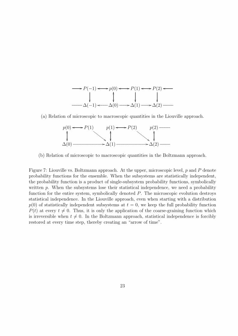
Figure 7: Liouville vs. Boltzmann approach. At the upper, microscopic level, p and P denoteprobability functions for the ensemble. When the subsystems are statistically independent,the probability function is a product of single-subsystem probability functions, symbolicallywritten p. When the subsystems lose their statistical independence, we need a probabilityfunction for the entire system, symbolically denoted P . The microscopic evolution destroysstatistical independence. In the Liouville approach, even when starting with a distributionp(0) of statistically independent subsystems at t = 0, we keep the full probability functionP (t) at every t 6= 0. Thus, it is only the application of the coarse-graining function whichis irreversible when t 6= 0. In the Boltzmann approach, statistical independence is forciblyrestored at every time step, thereby creating an “arrow of time”.

23

tation of the recurrent microscopic dynamics over a long period of time. On the contrary, itis the validity of the Stoßzahlansatz over any time scale which requires justification. Figure 6gives a sense that for the Kac ring, the time scale of relevance of the approximate dynamicsis very much shorter than the recurrence time.

In real physical many-body systems, the times of (approximate) recurrence are astronom-ically large as compared to typical time scales of thermodynamic experiments. Moreover,the chaotic character of the evolution will help maintain statistical independence over longintervals of time. This is illustrated by a computer simulation described in [3]: A gas isprepared in one side of a box which is separated in two compartments only accessible via asmall hole. During the simulation, the molecules pass through the small hole and the gas,slowly, distributes equally among both halves of the box toward statistical equilibrium. Ifnow the velocities are reversed, the gas indeed will return back to its initial condition withall molecules confined in one compartment. However, this time-reversed state is unstable: ifit is slightly perturbed, the system will remain in equilibrium. The fluctuations which de-correlate the prepared time-reversed state can be very small, but will get amplified throughthe chaotic nature of many-particle dynamics. This also explains why, in most cases, it isinfeasible to design “hidden controls” to create statistical dependence between molecules inthe initial state of a thermodynamic experiment.

Exercise 20. For given ∆ > 0, set up a Kac ring in its initial state S0 with a randomdistribution of markers and balls. First, turn the ring by one clockwise step into a new stateS1. Is ∆ more likely to increase or to decrease during this first step? Next, turn the ringone step anti-clockwise. Since the dynamics is time-reversible, we are reverting back to S0.Finally, turn the ring yet another step anti-clockwise into a state S−1. Is ∆ now more likelyto increase or to decrease?

10 Classroom notes

Students of mathematics and physics usually have to endure a long period of acquiring meth-ods, techniques and learning the necessary formalism before they can embark on tacklingdeep and fundamental problems which widen their intellectual horizon, not unlike the situa-tion of learning a foreign language where first one has to learn a substantial vocabulary beforemeeting and conversing with friends. However, very often these fundamental questions werethe very reason for the student to choose mathematics or physics as their subject.

These lecture notes try to engage students in very fundamental and deep concepts withonly very basic knowledge of mathematics. They developed when we were asked, independentof one another at our respective institutions, to teach a course for first year students that isorthogonal to the standard fare of Calculus and Linear Algebra, but rather stimulates thestudents’ interest, creative thinking, and exposure to various branches of mathematics.

Visits to the library soon revealed a wealth of elementary, but beautiful and deep problemsparadigmatic for many areas of pure mathematics. The supply on the applied side, however,is much more scarce. Where are the problems that require only elementary tools without

24

being isomorphic to some page of a reform-calculus textbook? That are applied withoutbeing narrow, that involve theory as well as computation or experiment? The obligatoryscan of the education section in the SIAM Reviews over the years also yields a wealth ofstimulating ideas. But for first years and still with some sense of broad relevance? Basicallynone.

Thus, we were thrilled when one of us (G.G.) discovered the Kac ring in one of theintroductory chapters of Dorfman’s book on nonequilibrium statistical mechanics [3]. Wehave now used this topic as a two or three week unit within our courses several times. Ourset of notes has subsequently grown from an extract of Dorfman to something more self-contained and, we hope, independently useful. While we might be pushing the notion of “forfirst year students” at times, we have written the text very much with first years in mindand believe that an experienced instructor will find it easy to distill the material down to anappropriate level of detail in a setting similar to ours.

In our experience, the topics covered in these notes can easily be taught in about 4–6lecture hours, depending on the depth of coverage and mathematical maturity of the students.We believe that the material offers two big pedagogical benefits.

First, very little prior hard knowledge is necessary. The concepts from combinatoricsand probability are so elementary that they can be taught “on the fly”, if necessary, orthe lectures may be embedded into a more general first introduction to combinatorics andprobability. For the most part, the discussion does not need calculus beyond elementarylimits which students will encounter early on in their regular first year calculus class; onlythe discussion of the continuum limit in Section 6 requires a deeper understanding of limits,but may safely be omitted or explored through computation. Section 5 is conceptionallyimportant and ultimately not more difficult than the derivation of ensemble averages in theprevious section, but the algebra can easily be intimidating and may be deemphasized.

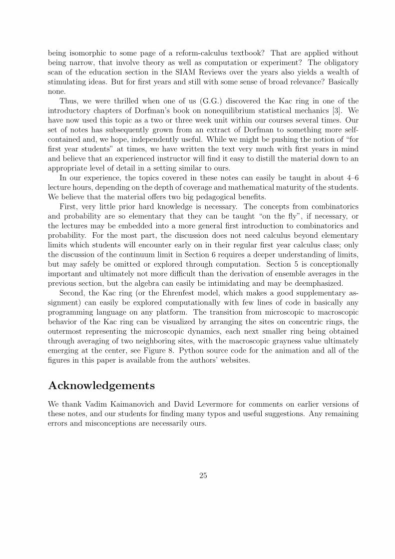
Second, the Kac ring (or the Ehrenfest model, which makes a good supplementary as-signment) can easily be explored computationally with few lines of code in basically anyprogramming language on any platform. The transition from microscopic to macroscopicbehavior of the Kac ring can be visualized by arranging the sites on concentric rings, theoutermost representing the microscopic dynamics, each next smaller ring being obtainedthrough averaging of two neighboring sites, with the macroscopic grayness value ultimatelyemerging at the center, see Figure 8. Python source code for the animation and all of thefigures in this paper is available from the authors’ websites.

Acknowledgements

We thank Vadim Kaimanovich and David Levermore for comments on earlier versions ofthese notes, and our students for finding many typos and useful suggestions. Any remainingerrors and misconceptions are necessarily ours.

25

Figure 8: Snapshot of the Kac ring animation, the markers being represented by the outer-most black-and-white ring, and the grayness colorcoded such that red represents δ = 1, bluerepresents δ = −1, and the white the equilibrium where δ = 0. The different rings showsuccessive coarse-graining via next-neighbor averaging in a binary tree fashion.

References

[1] D. Aldous and P. Diaconis, Shuffling cards and stopping times, Amer. Math. Monthly93 (1986), 333–348.

[2] C. Cercignani and E. Gabetta (eds.), “Transport Phenomena and Kinetic Theory –Applications to Gases, Semiconductors, Photons, and Biological Systems”, Birkhauser,Boston, 2007.

[3] J.R. Dorfman, “An introduction to chaos in nonequilibrium statistical dynamics”, Cam-bridge University Press, Cambridge, 1998.

[4] M. Dresden, New perspectives on Kac ring models, J. Stat. Phys. 46 (1987), 829–842.

[5] P. and T. Ehrenfest, Uber zwei bekannte Einwande gegen das Boltzmannsche H-

Theorem, Phys. Z. 8 (1907), 311–314.

[6] M. Kac, Some remarks on the use of probability in classical statistical mechanics, Acad.Roy. Belg. Bull. Cl. Sci. (5) 42 (1956), 356–361.

[7] J.L. Lebowitz, Macroscopic laws, microscopic dynamics, time’s arrow and Boltzmann’s

entropy, Phys. A 194 (1993), 1–27.

[8] D.J. Pine, J.P. Gollub, J.F. Brady, and A.M. Leshansky, Chaos and threshold for irre-

versibility in sheared suspensions, Nature 438 (2005), 997–1000.

[9] H. Poincare, Sur le problme des trois corps et les quations de la dynamique, Acta. Math.13 (1890), 1–270.

26

[10] I. Prigogine and I. Stengers, “Order out of chaos: Man’s new dialogue with nature”,Bantam Books, Toronto, 1984.

[11] J. Rothstein, Loschmidt’s and Zermelo’s paradoxes do not exist, Found. Phys. 4 (1974),83–89.

[12] L.S. Schulman, “Time’s arrow and quantum measurement”, Cambridge UniversityPress, Cambridge, 1997.

[13] E. Segre, “From falling bodies to radio waves”, W. H. Freeman, New York, 1984.

[14] C.E. Shannon, A mathematical theory of communication, The Bell System Technical J.27 (1948), 379–423 and 623–656.http://cm.bell-labs.com/cm/ms/what/shannonday/shannon1948.pdf

[15] T. Shinbrot, Drat such custard!, Nature 438 (2005), 922–923.

[16] L.N. Trefethen and L.M. Trefethen, How many shuffles to randomize a deck of cards?,R. Soc. Lond. Proc. A 456 (2000), 2561–2568.

[17] J. Uffink, “Boltzmann’s Work in Statistical Physics”, The Stanford Encyclopedia ofPhilosophy (Winter 2004 Edition), E.N. Zalta, (ed.).http://plato.stanford.edu/archives/win2004/entries/statphys-Boltzmann/

[18] E. Zermelo, Uber mechanische Erklarungen irreversibler Vorgange. Eine Antwort auf

Hrn. Boltzmann’s “Entgegnung”, Wiedemann Ann. 59 (1896), 793–801.

27