Both the quizzes and exams are closed book. However,

�For quizzes:

Formulas will be provided with quiz papers if there is any need.

�For exams (MD1, MD2, and Final):�For exams (MD1, MD2, and Final):

You may bring one 8.5” by 11” sheet of paper with formulas and notes written or typed on both sides to each exam.

Chapter 6

The Standard Deviation as a Ruler and the Normal Model Ruler and the Normal Model

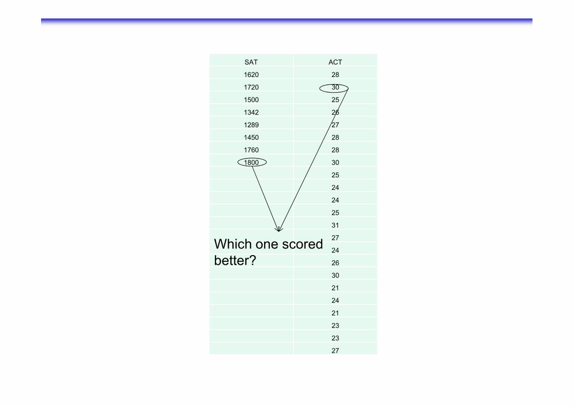
SAT ACT

1620 28

1720 30

1500 25

1342 26

1289 27

1450 28

1760 28

1800 30

25

24

2424

25

31

27

24

26

30

21

24

21

23

23

27

Which one scored better?

Standardizing with z-scores

� The trick in comparing very different-looking values is to standardize the values.

� Expressing the distances in standard deviations standardize the values.

� We compare individual data values to their mean, relative � We compare individual data values to their mean, relative to their standard deviation using the following formula:

� We call the resulting values standardized values, denoted as z. They can also be called z-scores.

z =

y − y( )s

Standardizing with z-scores (cont.)

� Standardized values have no units.

� z-scores measure the distance of each data value from the mean in standard deviations.

� A negative z-score tells us that the data value is � A negative z-score tells us that the data value is below the mean, while a positive z-score tells us that the data value is above the mean.

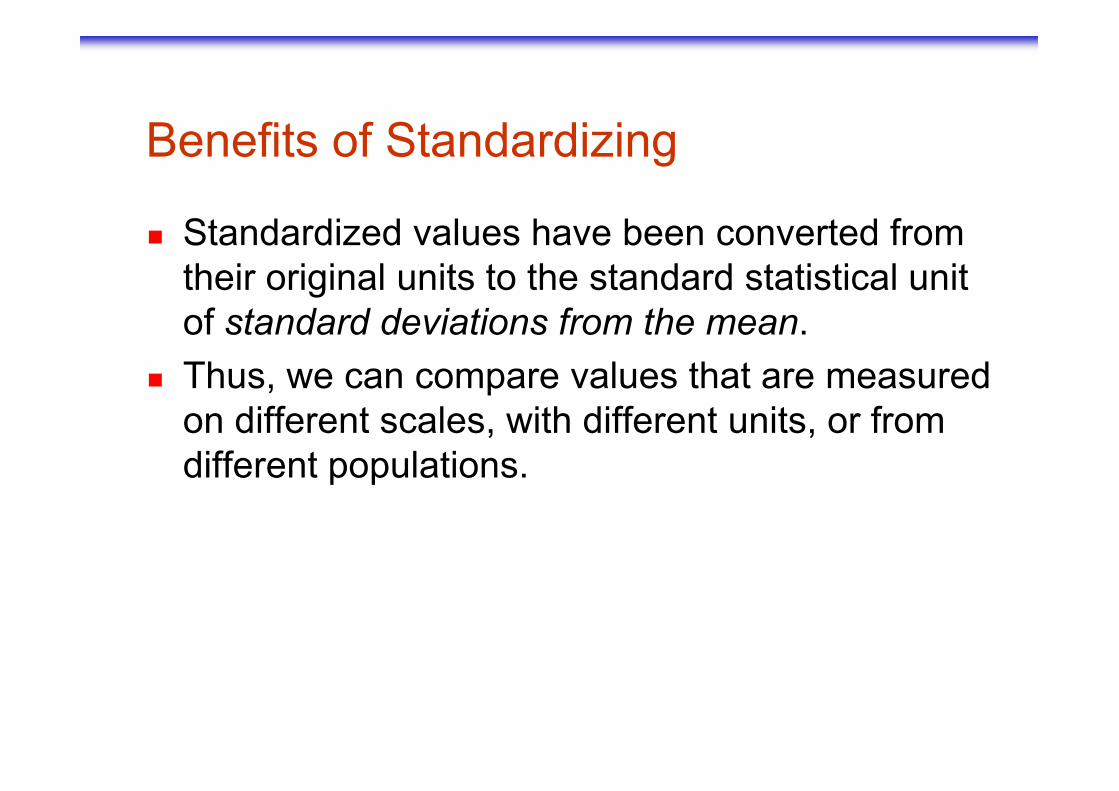
Benefits of Standardizing

� Standardized values have been converted from their original units to the standard statistical unit of standard deviations from the mean.

� Thus, we can compare values that are measured Thus, we can compare values that are measured on different scales, with different units, or from different populations.

Shifting Data

� Shifting data:

� Adding (or subtracting) a constant to every data value adds (or subtracts) the same constant to measures of position.

Adding (or subtracting) a constant to each � Adding (or subtracting) a constant to each value will increase (or decrease) measures of position: center, percentiles, max or min by the same constant.

� Its shape and spread - range, IQR, standard deviation - remain unchanged.

Shifting Data (cont.)

� The following histograms show a shift from men’s actual weights to kilograms above recommended weight:

Mean weight 82.36 kg

To compare their weights with recommended maximum weight of 74 kg, we subtract this value from each weight

kg

Rescaling Data

� Rescaling data:

� When we multiply (or divide) all the data values by any constant, all measures of position (such as the mean, median, and percentiles) and as the mean, median, and percentiles) and measures of spread (such as the range, the IQR, and the standard deviation) are multiplied (or divided) by that same constant.

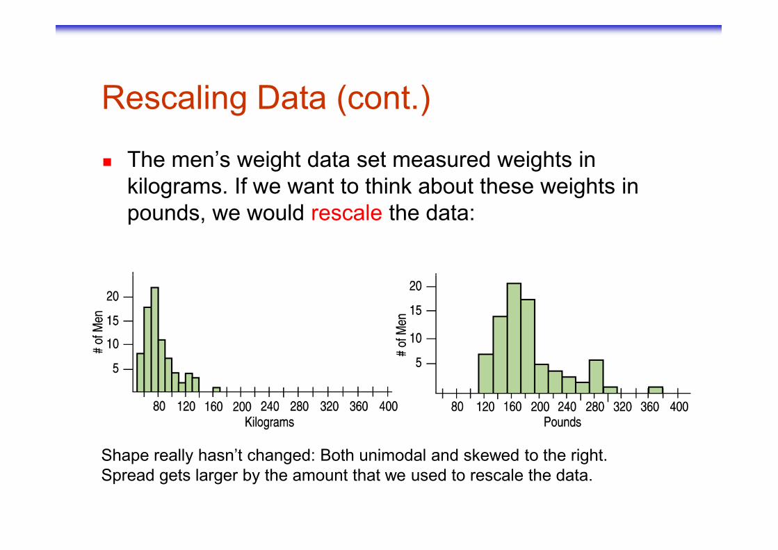
Rescaling Data (cont.)

� The men’s weight data set measured weights in kilograms. If we want to think about these weights in pounds, we would rescale the data:

Shape really hasn’t changed: Both unimodal and skewed to the right.Spread gets larger by the amount that we used to rescale the data.

Just checking

� In 1995 the educational testing service (ETS) adjusted the scores of SAT tests. Before ETS recentered the SAT verbal test, the mean of all test scores was 450.

A) How would adding 50 points to each score affect the mean?

B) The standard deviation was 100 points. What would the standard deviation be after adding 50 points?deviation be after adding 50 points?

C) Suppose we drew box-plots of test takers’ scores a year before and a year after the recentering. How would the box-plots of the two years differ?

Just checking

� In 1995 the educational testing service (ETS) adjusted the scores of SAT tests. Before ETS recentered the SAT verbal test, the mean of all test scores was 450.

A) How would adding 50 points to each score affect the mean?

New mean= 450+50

B) The standard deviation was 100 points. What would the standard B) The standard deviation was 100 points. What would the standard deviation be after adding 50 points?

New std= 100

C) Suppose we drew box-plots of test takers’ scores a year before and a year after the recentering. How would the box-plots of the two years differ?

All measures in the box-plot would increase by 50 points after recentering.

Back to z-scores

� Standardizing data into z-scores shifts the data by subtracting the mean and rescales the values by dividing by their standard deviation.

� Standardizing into z-scores does not change Standardizing into z-scores does not change the shape of the distribution.

� Standardizing into z-scores changes the centerby making the mean 0.

� Standardizing into z-scores changes the spread by making the standard deviation 1.

When Is a z-score BIG?

� A z-score gives us an indication of how unusual a value is because it tells us how far it is from the mean.

� Remember that a negative z-score tells us that Remember that a negative z-score tells us that the data value is below the mean, while a positive z-score tells us that the data value is above the mean.

� The larger a z-score is (negative or positive), the more unusual it is.

� To say more about how big we expect a z-score to be, we need to model the data’s distribution.

� A model will let us say much more precisely how often we’d be likely to see z-scores of different often we’d be likely to see z-scores of different sizes.

� Of course, like all models of the real world, the model will be wrong-wrong in the sense that it can’t match reality exactly. But it can still be useful.

When Is a z-score Big? (cont.)

� There is no universal standard for z-scores, but there is a model that shows up over and over in Statistics.

� This model is called the Normal model (You may have heard of “bell-shaped curves.”).have heard of “bell-shaped curves.”).

� Normal models are appropriate for distributions whose shapes are unimodal and roughly symmetric.

� These distributions provide a measure of how extreme a z-score is.

When Is a z-score Big? (cont.)

� There is a Normal model for every possible combination of mean and standard deviation.

� We write N(µ,σ) to represent a Normal model with a mean of µ and a standard deviation of σ.

We use Greek letters because this mean and � We use Greek letters because this mean and standard deviation do not come from data—they are numbers (called parameters) that specify the model.

When Is a z-score Big? (cont.)

� Summaries of data, like the sample mean and standard deviation, are written with Latin letters. Such summaries of data are called statistics.

� When we standardize Normal data, we still call the standardized value a z-score, and we write standardized value a z-score, and we write

yz

µ

σ

−=

When Is a z-score Big? (cont.)

� Once we have standardized, we need only one model:

� The N(0,1) model is called the standard Normal model (or the standard Normal Normal model (or the standard Normal distribution).

� Be careful—don’t use a Normal model for just any data set, since standardizing does not change the shape of the distribution.

When Is a z-score Big? (cont.)

� When we use the Normal model, we are assuming the distribution is Normal.

� We cannot check this assumption in practice, so we check the following condition:we check the following condition:

� Nearly Normal Condition: The shape of the data’s distribution is unimodal and symmetric.

� This condition can be checked by making a histogram or a Normal probability plot (to be explained later).

The 68-95-99.7 Rule (Empirical Rule)

� Normal models give us an idea of how extreme a value is by telling us how likely it is to find one that far from the mean.

� We can find these numbers precisely, but until We can find these numbers precisely, but until then we will use a simple rule that tells us a lot about the Normal modelG

The 68-95-99.7 Rule (cont.)

� It turns out that in a Normal model:

� about 68% of the values fall within one standard deviation of the mean;

� about 95% of the values fall within two � about 95% of the values fall within two standard deviations of the mean; and,

� about 99.7% (almost all!) of the values fall within three standard deviations of the mean.

The 68-95-99.7 Rule (cont.)

� The following shows what the 68-95-99.7 Rule tells us:

Just checking

� As a group, the Dutch are among the tallest people in the world. The average Dutch man is 184 cm tall-just over 6 feet. If a Normal model is appropriate and the standard deviation for men is about 8 cm, what percentage of all Dutch men will be over 2 meters?Dutch men will be over 2 meters?

� Solution:� 184-2*8=168 cm

� 184+2*8=200( 2 meters)

� 95% of the Dutch men have heights between 168 cm and 200 cm.

� We expect 5% of the men to be more than 200 cm or less than 168 cm.

� So 2.5% of the men are expected to be more than 2 meters.

Just Checking

� Suppose it takes you 20 minutes, on average, to drive to school, with a standard deviation of 2 minutes. Suppose a Normal model is appropriate for the distributions of driving times.

A) How often will you drive at school less than 22 minutes?

84% of time

B) How often will it take you more than 24 minutes?

2.5% of time

The First Three Rules for Working with Normal Models

� Make a picture.

� Make a picture.

� Make a picture.

� And, when we have data, make a histogram to check the Nearly Normal Condition to make sure we can use the Normal model to model the distribution.

Finding Normal Percentiles by Hand

� When a data value doesn’t fall exactly 1, 2, or 3 standard deviations from the mean, we can look it up in a table of Normal percentiles.

� Table Z in Appendix D provides us with normal Table Z in Appendix D provides us with normal percentiles, but many calculators and statistics computer packages provide these as well.

Finding Normal Percentiles by Hand (cont.)

� Table Z is the standard Normal table. We have to convert our data to z-scores before using the table.

� The figure shows us how to find the area to the left when we have a z-score of 1.80:

Finding Normal Percentiles Using Technology

� Many calculators and statistics programs have the ability to find normal percentiles for us.

� The ActivStats Multimedia Assistant offers two methods for finding normal percentiles:

� The “Normal Model Tool” makes it easy to see how � The “Normal Model Tool” makes it easy to see how areas under parts of the Normal model correspond to particular cut points.

� There is also a Normal table in which the picture of the normal model is interactive.

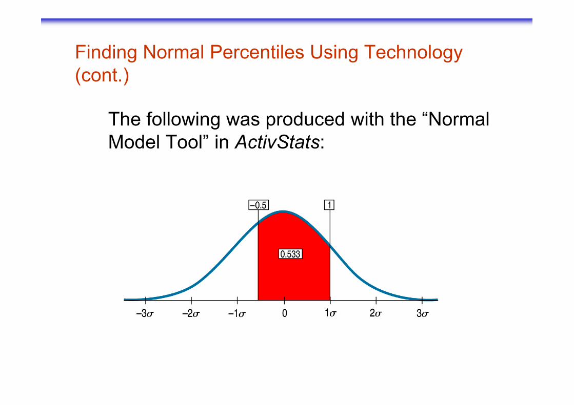
Finding Normal Percentiles Using Technology (cont.)

The following was produced with the “Normal Model Tool” in ActivStats:

From Percentiles to Scores: z in Reverse

� Sometimes we start with areas and need to find the corresponding z-score or even the original data value.

� Example: What z-score represents the first Example: What z-score represents the first quartile in a Normal model?

From Percentiles to Scores: z in Reverse (cont.)

� Look in Table Z for an area of 0.2500.

� The exact area is not there, but 0.2514 is pretty close.

� This figure is associated with z = -0.67, so the first quartile is 0.67 standard deviations below the mean.

Are You Normal? Normal Probability Plots

� When you actually have your own data, you must check to see whether a Normal model is reasonable.

� Looking at a histogram of the data is a good way Looking at a histogram of the data is a good way to check that the underlying distribution is roughly unimodal and symmetric.

� A more specialized graphical display that can help you decide whether a Normal model is appropriate is the Normal probability plot.

� If the distribution of the data is roughly Normal, the Normal probability plot approximates a

Are You Normal? Normal Probability Plots (cont)

the Normal probability plot approximates a diagonal straight line. Deviations from a straight line indicate that the distribution is not Normal.

� Nearly Normal data have a histogram and a Normal probability plot that look somewhat like this example:

Are You Normal? Normal Probability Plots (cont)

These two values are a bit lower than we’d expect of the lowest two values in a Normal model.

� A skewed distribution might have a histogram and Normal probability plot like this for which 68-95-99.7 rule would not be accurate.

Are You Normal? Normal Probability Plots (cont)

What Can Go Wrong?

� Don’t use a Normal model when the distribution is not unimodal and symmetric.

Ex. 6.3

� Here are the summary statistics for the weekly payroll of a small company: lowest salary=$300, mean salary=$700, median=$500, range=$1200, IQR=$600, first quartile=$350, standard dev.=$400.first quartile=$350, standard dev.=$400.

a) Do you think the distribution of salaries is symmetric, skewed to the left, or skewed to the right?

It is skewed to the right since mean > median

Ex. 6.3 (cont.)b) Between what two values are the middle 50% of the salaries found?

$350, $250(IQR-350)

c) Suppose business has been good and the company gives every employee a $50 raise. Tell the new value of each summary statistics.new value of each summary statistics.

Except the standard deviation every statistics will increase 50 points. Standard dev. Will remain unchanged.d) Instead, suppose the company gives each employee a 10% raise. Tell the new value of each of the summary statistics.

Ex. 6.3 (cont.)d) Instead, suppose the company gives each employee a 10% raise. Tell the new value of each of the summary statistics.

New mean= 700+700*0.10=770

New median=500+500*0.1=550New median=500+500*0.1=550

New min=300+300*.1=330

New range=1200+1200*.10=1320

New IQR=600+600*.10=660

New std=400

Ex. 6.10

� Cars currently sold in the US have an average of 135 horsepower, with a standard deviation of 40 horsepower. What is the z-score for a car with 195 horse power?

Z=(195-135)/40=1.5

Ex. 6.12

� People with z-scores greater than 2.5 on an IQ test are sometimes classified as geniuses. If IQ test scores have a mean of 100 and a std. dev. of 16 points, what IQ score do you need to be considered a score do you need to be considered a genious?

2.5=(x-100)/16 x=140

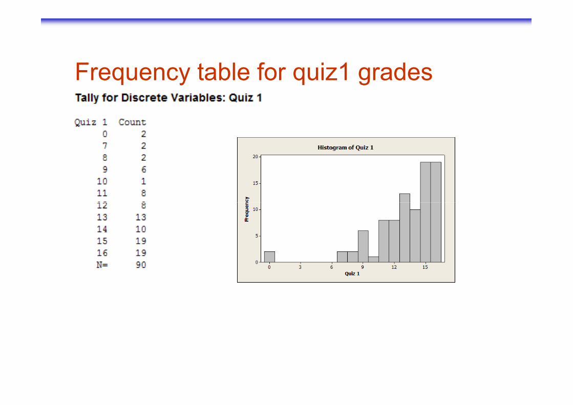
Frequency table for quiz1 grades

Descriptive statistics for Grades by sections

Box plots for Grades by sections

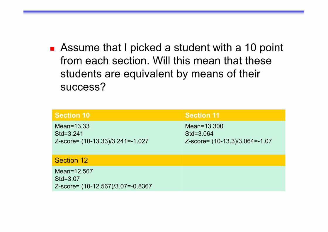
� Assume that I picked a student with a 10 point from each section. Will this mean that these students are equivalent by means of their success?

Section 10 Section 11Section 10 Section 11

Mean=13.33Std=3.241Z-score= (10-13.33)/3.241=-1.027

Mean=13.300Std=3.064Z-score= (10-13.3)/3.064=-1.07

Section 12

Mean=12.567Std=3.07Z-score= (10-12.567)/3.07=-0.8367

Ex. 6.42� In a standard Normal model, what value(s) of z

cut(s) off the region described?

A) The lowest 12%

-1.175

B) The highest 30%B) The highest 30%

0.53

C) The highest 7%

1.47

D) The middle 50%

(-0.67, 0.67)

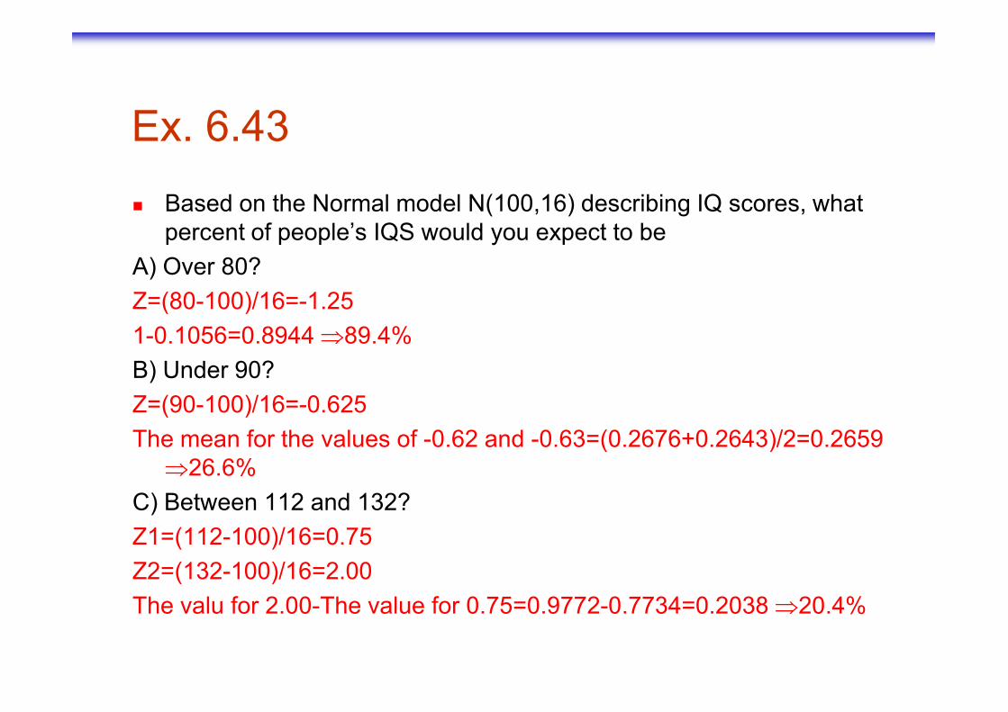
Ex. 6.43

� Based on the Normal model N(100,16) describing IQ scores, what percent of people’s IQS would you expect to be

A) Over 80?

Z=(80-100)/16=-1.25

1-0.1056=0.8944 ⇒89.4%

B) Under 90?

Z=(90-100)/16=-0.625

The mean for the values of -0.62 and -0.63=(0.2676+0.2643)/2=0.2659⇒26.6%

C) Between 112 and 132?

Z1=(112-100)/16=0.75

Z2=(132-100)/16=2.00

The valu for 2.00-The value for 0.75=0.9772-0.7734=0.2038 ⇒20.4%

Ex. 6.27� Environmental protection agency (EPA) fuel economy

estimates for automobile models tested recently predicted a mean of 24.8 mpg and a standard deviation of 6.2 mpg for highway driving. Assume that the distribution is mound-shaped(i.e; Normal model applies)

A) Draw the model for auto fuel economy. Clearly label it showing what the 68-95-99.7 rule predicts about miles per gallon.

B) In what interval would you expect the central 68% of autos to be found?

C) About what percent of autos should get more than 31 mpg?

D) About what percent of autos should get between 31 and 37 mpg?

E) Describe the gas mileage of the worst 2.5% of all cars?

What Can Go Wrong? (cont.)

� Don’t use the mean and standard deviation when outliers are present—the mean and standard deviation can both be distorted by outliers.

� Don’t round your results in the middle of a Don’t round your results in the middle of a calculation.

� Don’t worry about minor differences in results.

What have we learned?

� The story data can tell may be easier to understand after shifting or rescaling the data.

� Shifting data by adding or subtracting the same amount from each value affects measures of amount from each value affects measures of center and position but not measures of spread.

� Rescaling data by multiplying or dividing every value by a constant changes all the summary statistics—center, position, and spread.

What have we learned? (cont.)

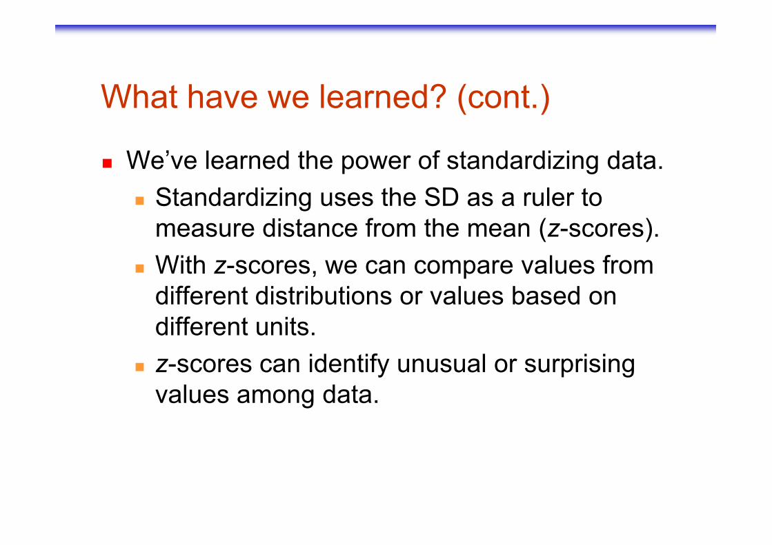
� We’ve learned the power of standardizing data.

� Standardizing uses the SD as a ruler to measure distance from the mean (z-scores).

� With z-scores, we can compare values from � With z-scores, we can compare values from different distributions or values based on different units.

� z-scores can identify unusual or surprising values among data.

� We’ve learned that the 68-95-99.7 Rule can be a useful rule of thumb for understanding distributions:

� For data that are unimodal and symmetric,

What have we learned? (cont.)

For data that are unimodal and symmetric, about 68% fall within 1 SD of the mean, 95% fall within 2 SDs of the mean, and 99.7% fall within 3 SDs of the mean.

What have we learned? (cont.)

� We see the importance of Thinking about whether a method will work:

� Normality Assumption: We sometimes work with Normal tables (Table Z). These tables are with Normal tables (Table Z). These tables are based on the Normal model.

� Data can’t be exactly Normal, so we check the Nearly Normal Condition by making a histogram (is it unimodal, symmetric and free of outliers?) or a normal probability plot (is it straight enough?).